Chapter 8 Conditional Random Fields - SNU · Fall 2010 Graduate Course on Dynamic Learning Chapter8:ConditionalRandomFieldsChapter 8: Conditional Random Fields November1,2010November

Fall 2010 Graduate Course on Dynamic Learning

Chapter 8: Conditional Random FieldsChapter 8: Conditional Random Fields

November 1, 2010November 1, 2010

Byoung-Tak Zhang

School of Computer Science and Engineering &Cognitive Science and Brain Science Programs

Seoul National University

http://bi.snu.ac.kr/~btzhang/

OverviewOverview

• Motivating Applications– Sequence Segmentation and Labelingq g g

• Generative vs. Discriminative ModelsHMM MEMM– HMM, MEMM

• CRF– From MRF to CRF

Learning Algorithms– Learning Algorithms• HMM vs. CRF

2

Motivating Application:Sequence Labeling

• Pos Tagging[He/PRP] [reckons/VBZ] [the/DT] [current/JJ][He/PRP] [reckons/VBZ] [the/DT] [current/JJ] [account/NN] [deficit/NN] [will/MD] [narrow/VB] [to/TO] [only/RB] [#/#] [1.8/CD] [billion/CD] [in/IN] [September/NNP] [./.]

• Term ExtractionRockwell International Corp.’s Tulsa unit said it signed a tentative agreement extending its contract with Boeing Co.to provide structural parts for Boeing’s 747 jetliners.

• Information Extraction from Company Annual Report

3

Sequence Segmenting and LabelingSequence Segmenting and Labeling

• Goal: mark up sequences with content tags• Goal: mark up sequences with content tags• Computational linguistics

T t d h i– Text and speech processing– Topic segmentation

Part of speech (POS) tagging– Part-of-speech (POS) tagging– Information extraction– Syntactic disambiguationSyntactic disambiguation

• Computational biology– DNA and protein sequence alignmentN a d p o e seque ce a g e– Sequence homolog searching in databases– Protein secondary structure prediction

RNA d t t l i– RNA secondary structure analysis

Binary Classifier vs. Sequence yLabeling

• Case restoration– jack utilize outlook express to retrieve emailsj p– E.g. SVMs vs. CRFs

- Jack utilize outlook express to retrieve emails.

+

Jack Utilize Outlook Express To Receive Emails

jack

JACK

utilize

UTILIZE

outlook

OUTLOOK

express

EXPRESS

to

TO

receive

RECEIVE

emails

EMAILS

5

Sequence Labeling Models: Overviewq g

• HMM– Generative model– E.g. Ghahramani (1997), Manning and Schutze (1999)

• MEMM– Conditional model

E B d Pi (1996) M C ll d F i (2000)– E.g. Berger and Pietra (1996), McCallum and Freitag (2000)• CRFs

C diti l d l ith t l b l bi bl– Conditional model without label bias problem– Linear-Chain CRFs

• E.g. Lafferty and McCallum (2001), Wallach (2004)E.g. Lafferty and McCallum (2001), Wallach (2004)

– Non-Linear Chain CRFs• Modeling more complex interaction between labels: DCRFs, 2D-CRFs

S d C ll ( ) h d i ( )

6

• E.g. Sutton and McCallum (2004), Zhu and Nie (2005)

Generative Models: HMM

• Based on joint probability distribution P(y,x)j p y (y )• Includes a model of P(x) which is not needed for

classification• Interdependent features

– either enhance model structure to represent them (complexity problems)complexity problems)

– or make simplifying independence assumptions (e.g. naive Bayes)

Hidd M k d l (HMM ) d t h ti• Hidden Markov models (HMMs) and stochastic grammars– Assign a joint probability to paired observation and labelAssign a joint probability to paired observation and label

sequences– The parameters typically trained to maximize the joint

lik lih d f t i llikelihood of train examples

Hidden Markov ModelHidden Markov Model

( ) ( ) ( | ) ( | ) ( | )n

P s x P s P x s P s s P x s= ∏1 1 1 12

( , ) ( ) ( | ) ( | ) ( | )i i i ii

P s x P s P x s P s s P x s−=

= ∏

Cannot represent multiple interacting (overlapping) features or long range dependences between observed elements.

8

Conditional Models• Difficulties and disadvantages of generative models

Need to enumerate all possible observation sequences– Need to enumerate all possible observation sequences– Not practical to represent multiple interacting features or long-range

dependencies of the observations– Very strict independence assumptions on the observations

• Conditional ModelsConditional probability P(y|x) rather than joint probability P(y x) where y =– Conditional probability P(y|x) rather than joint probability P(y, x) where y = label sequence and x = observation sequence.

– Based directly on conditional probability P(y|x)– Need no model for P(x)– Specify the probability of possible label sequences given an observation

sequence– Allow arbitrary, non-independent features on the observation sequence X– The probability of a transition between labels may depend on past and future

observations– Relax strong independence assumptions in generative models

Discriminative Models: MEMM• Maximum entropy Markov model (MEMM)

– Exponential modelp• Given a training set (X, Y) of observation sequences X and label

sequences Y:– Train a model θ that maximizes P(Y|X, θ)– For a new data sequence x, the predicted label y maximizes P(y|x, θ)– Notice the per-state normalization

• MEMMs have all the advantages of conditional models• Per-state normalization: all the mass that arrives at a state must bePer state normalization: all the mass that arrives at a state must be

distributed among the possible successor states (“conservation of score mass”)S bj t t L b l Bi P bl• Subject to Label Bias Problem– Bias toward states with fewer outgoing transitions

Maximum Entropy Markov ModelMaximum Entropy Markov Model

( | ) ( | ) ( | )n

P P P∏1 1 12

( | ) ( | ) ( | , )i i ii

P s x P s x P s s x−=

= ∏Label bias problem: the probability transitions leaving any given state must sum to one

11

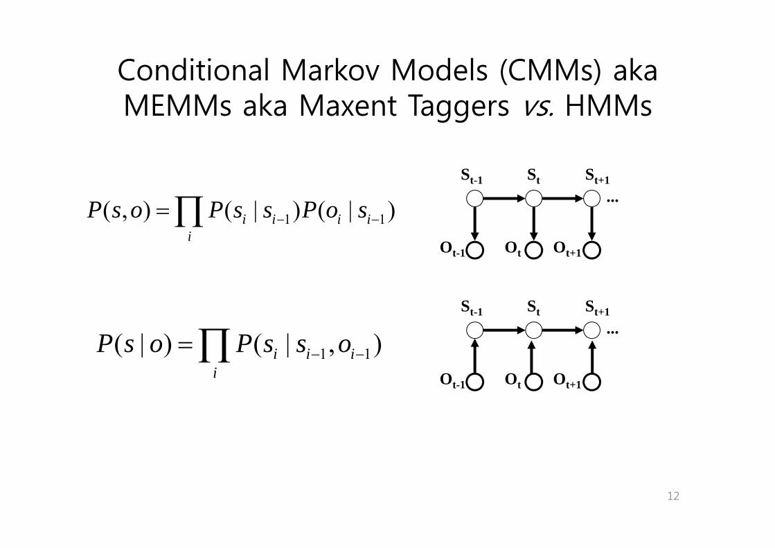
Conditional Markov Models (CMMs) aka MEMMs aka Maxent Taggers vs. HMMs

St-1 St St+1...( ) ( | ) ( | )P s o P s s P o s= ∏

Ot Ot+1Ot-1

1 1( , ) ( | ) ( | )i i i ii

P s o P s s P o s− −= ∏

St-1 St St+1...

( | ) ( | )P P∏Ot Ot+1Ot-1

1 1( | ) ( | , )i i ii

P s o P s s o− −= ∏

12

MEMM to CRFsMEMM to CRFsexp( ( ))f x y yλ∑ 1

1 1 1,

exp( ( , , ))( ... | ... ) ( | )

( )

i i j j ji

n n j j jj j j

f x y yP y y x x P y y x

Z xλ

λ −

−= =∑

∏ ∏

exp( ( , ))i iFλ∑ x y1, where ( , ) ( , , )

( )

i ii

i i j j jjj

j

F f x y yZ xλ

−= =∑

∑∏x y

exp( ( , ))i iFλ∑ x yNew model

j

p( ( , ))

( )

i ii

Zλ

∑ y

x

New model

13

( )Zλ x

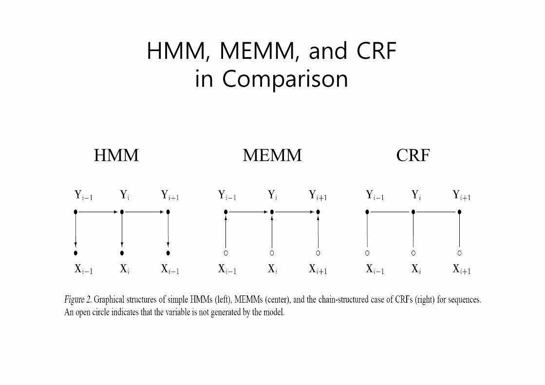
HMM, MEMM, and CRF , ,in Comparison

CHMM MEMM CRF

Conditional Random FieldConditional Random Field (CRF)( )

Random FieldRandom Field

Markov Random Field

• Random Field: Let be a family of random variables defined on the set S in which each random

},...,,{ 21 MFFFF =variables defined on the set S , in which each random variable takes a value in a label set L. The family Fis called a random field.

iF if

• Markov Random Field: F is said to be a Markov random field on S with respect to a neighborhood system N if and only if it satisfies the Markov property.– undirected graph for joint probability p(x)

ll di t b bili ti i t t ti– allows no direct probabilistic interpretation– define potential functions Ψ on maximal cliques A

• map joint assignment to non-negative real numberp j g g• requires normalisation

p(x) =1Z

ΨA (xA )∏ Z = ΨA (xA )∏∑p( )Z A ( A )

A∏ A ( A )

A∏

x∑

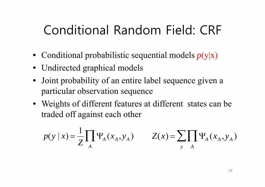
Conditional Random Field: CRFConditional Random Field: CRF

• Conditional probabilistic sequential models p(y|x)• Undirected graphical modelsg p• Joint probability of an entire label sequence given a

particular observation sequenceparticular observation sequence • Weights of different features at different states can be

traded off against each othertraded off against each other

p(y | x) =1

Ψ (x y )∏ Z(x) = Ψ (x y )∏∑p(y | x) =Z

ΨA (xA ,yA )A

∏ Z(x) = ΨA (xA , yA )A

∏y

∑

18

Example of CRFsExample of CRFs

Definition of CRFs

X is a random variable over data sequences to be labeledX is a random variable over data sequences to be labeledY is a random variable over corresponding label sequences

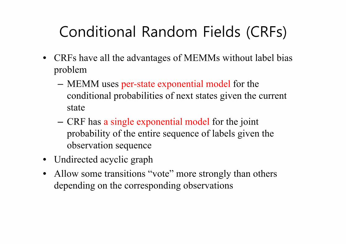
Conditional Random Fields (CRFs)( )

• CRFs have all the advantages of MEMMs without label bias blproblem

– MEMM uses per-state exponential model for the conditional probabilities of next states given the currentconditional probabilities of next states given the current state

– CRF has a single exponential model for the joint– CRF has a single exponential model for the joint probability of the entire sequence of labels given the observation sequenceq

• Undirected acyclic graph• Allow some transitions “vote” more strongly than others g y

depending on the corresponding observations

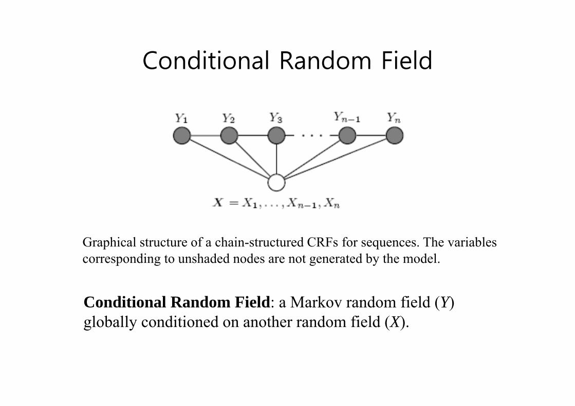
Conditional Random FieldConditional Random Field

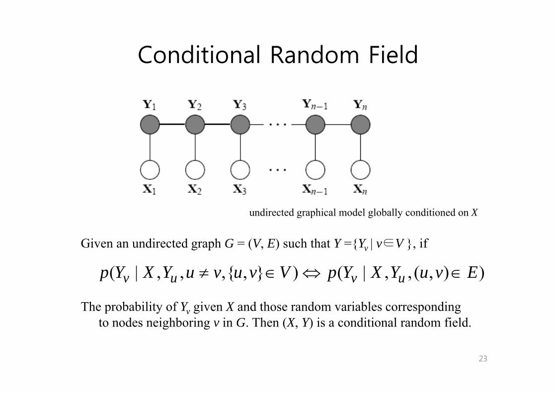
Graphical structure of a chain-structured CRFs for sequences. The variables p qcorresponding to unshaded nodes are not generated by the model.

Conditional Random Field: a Markov random field (Y) globally conditioned on another random field (X).

Conditional Random FieldConditional Random Field

Gi di t d h G (V E) h th t Y {Y | ∈V } if

undirected graphical model globally conditioned on X

Given an undirected graph G = (V, E) such that Y ={Yv | v∈V }, if

( | , , ,{ , } ) ( | , , ( , ) )v u v up Y X Y u v u v V p Y X Y u v E≠ ∈ ⇔ ∈

The probability of Yv given X and those random variables corresponding to nodes neighboring v in G. Then (X, Y) is a conditional random field.

23

Conditional Distribution

If the graph G = (V, E) of Y is a tree, the conditional distribution over the label sequence Y = y given X = x by fundamental theorem of randomlabel sequence Y = y, given X = x, by fundamental theorem of random fields is:

(y | x) exp ( y | x) ( y | x)λ μ⎛ ⎞

∝ +⎜ ⎟∑ ∑p f e g v

x is a data sequence

(y | x) exp ( , y | , x) ( , y | , x)θ λ μ∈ ∈

∝ +⎜ ⎟⎝ ⎠∑ ∑k k e k k v

e E,k v V ,kp f e g v

y is a label sequence v is a vertex from vertex set V = set of label random variablese is an edge from edge set E over Vg gfk and gk are given and fixed. gk is a Boolean vertex feature; fk is a

Boolean edge featurek is the number of features

1 2 1 2( , , , ; , , , ); andn n k kθ λ λ λ μ μ μ λ μ=k is the number of features

are parameters to be estimatedy|e is the set of components of y defined by edge ey| is the set of components of y defined by vertex vy|v is the set of components of y defined by vertex v

Conditional Distribution (cont’d)( )

• CRFs use the observation-dependent normalization Z(x) for the

conditional distributions:

( | ) ( | ) ( |1 )λ⎛ ⎞⎜ ⎟∑ ∑f(y | x) exp ( , y | , x) ( , y |

(x), x)θ λ μ

∈ ∈

= +⎜ ⎟⎝ ⎠∑ ∑k k e k k v

e E,k v V ,kp f e g v

Z

Z(x) is a normalization over the data sequence x

Conditional Random Fields

/k/ /k/ /iy/ /iy/ /iy/

X X X X X

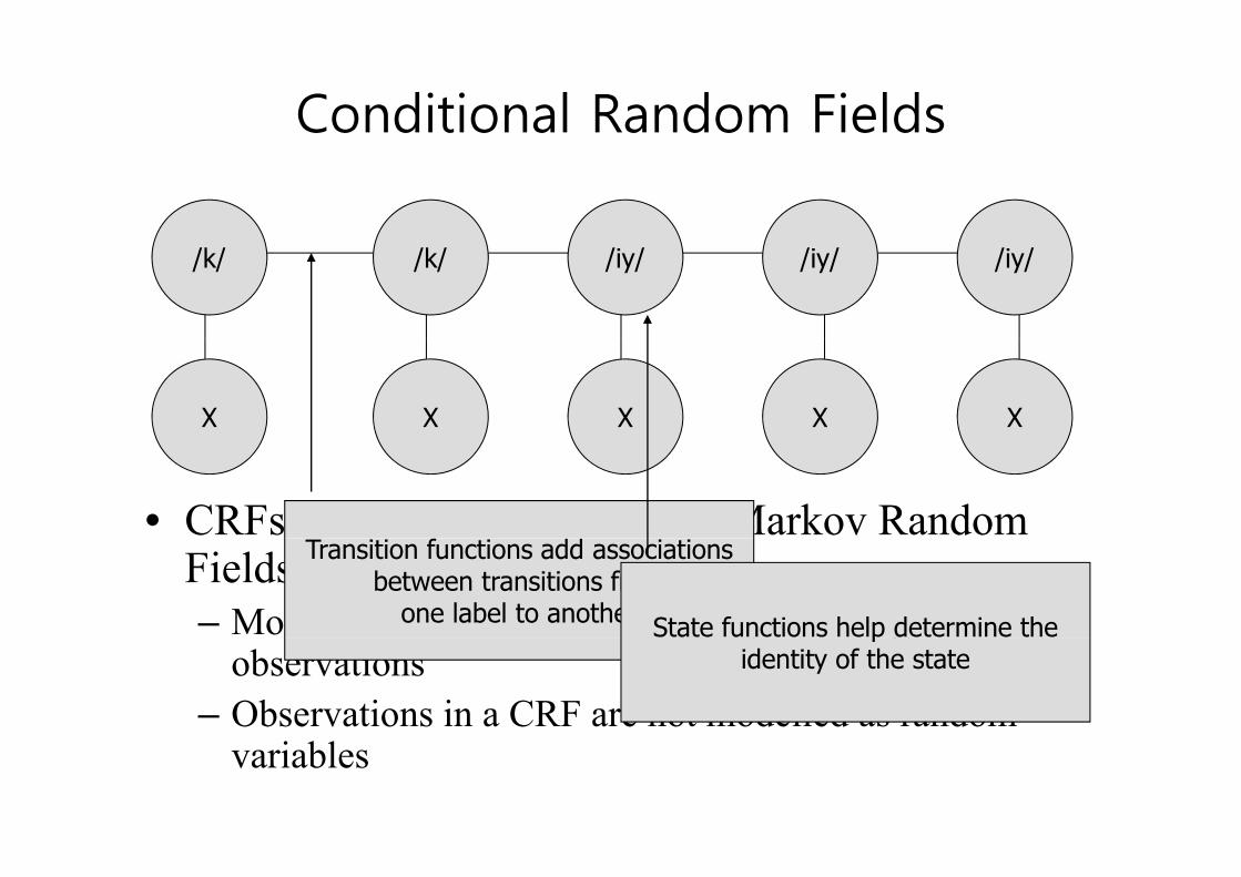
• CRFs are based on the idea of Markov Random Fields– Modelled as an undirected graph connecting labels with

Transition functions add associationsbetween transitions from

one label to another State functions help determine theg p gobservations

– Observations in a CRF are not modelled as random

pidentity of the state

variables

Conditional Random FieldsConditional Random Fields

)),,(),((exp)|(

1yyxgyxfP t i j

ttjjtii∑∑ ∑ −+ μλ

)()|(

xZxyP t i j=

State Feature FunctionState Feature Weight Transition Feature FunctionTransition Feature WeightHammersley-Clifford Theorem states that a

State Feature Function

f([x is stop], /t/)λ=10

One possible weight value

g(x, /iy/,/k/)

Transition Feature Weight

μ=4random field is an MRF iff it can be described in the above form

One possible state feature functionFor our attributes and labels

One possible weight valuefor this state feature

(Strong)

One possible transition feature function

Indicates /k/ followed by /iy/

One possible weight valuefor this transition feature

the above formThe exponential is the sum of the clique potentials of the undirected graphthe undirected graph

Conditional Random Fields

• Each attribute of the data we are trying to model fits y ginto a feature function that associates the attribute and a possible label– A positive value if the attribute appears in the data– A zero value if the attribute is not in the data

• Each feature function carries a weight that gives the strength of that feature function for the proposed label– High positive weights indicate a good association between

the feature and the proposed labelHigh negative weights indicate a negative association– High negative weights indicate a negative association between the feature and the proposed label

– Weights close to zero indicate the feature has little or no gimpact on the identity of the label

Formally …. Definitiony• CRF is a Markov random field. • By the Hammersley-Clifford theorem, the probability of a label can beBy the Hammersley Clifford theorem, the probability of a label can be

expressed as a Gibbs distribution, so that1( | , , ) exp( ( , ))j jp y x F y xλ μ λ= ∑

|

( | , , ) p( ( , ))

( , ) ( , , )

j jj

n

j j c

p y yZ

F y x f y x i

μ

=

∑

∑ |1

( , ) ( , , )j j ci

y f y=∑

• What is clique?

clique

1

• By only taking consideration of the one-node and two-node cliques, we have

| |1( | , , ) exp( ( , , ) ( , , ))j j e k k s

j kp y x t y x i s y x i

Zλ μ λ μ= +∑ ∑

29

Definition (cont )Definition (cont.)

Moreover, let us consider the problem in a first-order chain model, we have

1 ∑ ∑11( | , , ) exp( ( , , , ) ( , , ))j j i i k k i

j kp y x t y y x i s y x i

Zλ μ λ μ−= +∑ ∑

For simplifying description, let fj(y, x) denote tj(yi-1, yi, x, i) and sk(yi, x, i)

11( | , , ) exp( ( , ))j jj

p y x F y xZ

λ μ λ= ∑

|1

( , ) ( , , )n

j j ci

F y x f y x i=

= ∑

30

LabelingLabeling

• In labeling, the task is to find the label sequence that has the largest probability

• Then the key is to estimate the parameter lambda

ˆ arg max ( | ) arg max( ( , ))y y

y p y x F y xλ λ= = ⋅

1( | , , ) exp( ( , ))j jj

p y x F y xZ

λ μ λ= ∑j

31

OptimizationOptimization

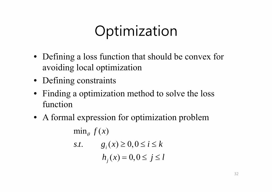
• Defining a loss function that should be convex for avoiding local optimization

• Defining constraints• Finding a optimization method to solve the lossFinding a optimization method to solve the loss

function• A formal expression for optimization problem• A formal expression for optimization problem

min ( )f xθ

. . ( ) 0,0( ) 0,0

i

j

s t g x i kh x j l

≥ ≤ ≤

= ≤ ≤

32

( )j j

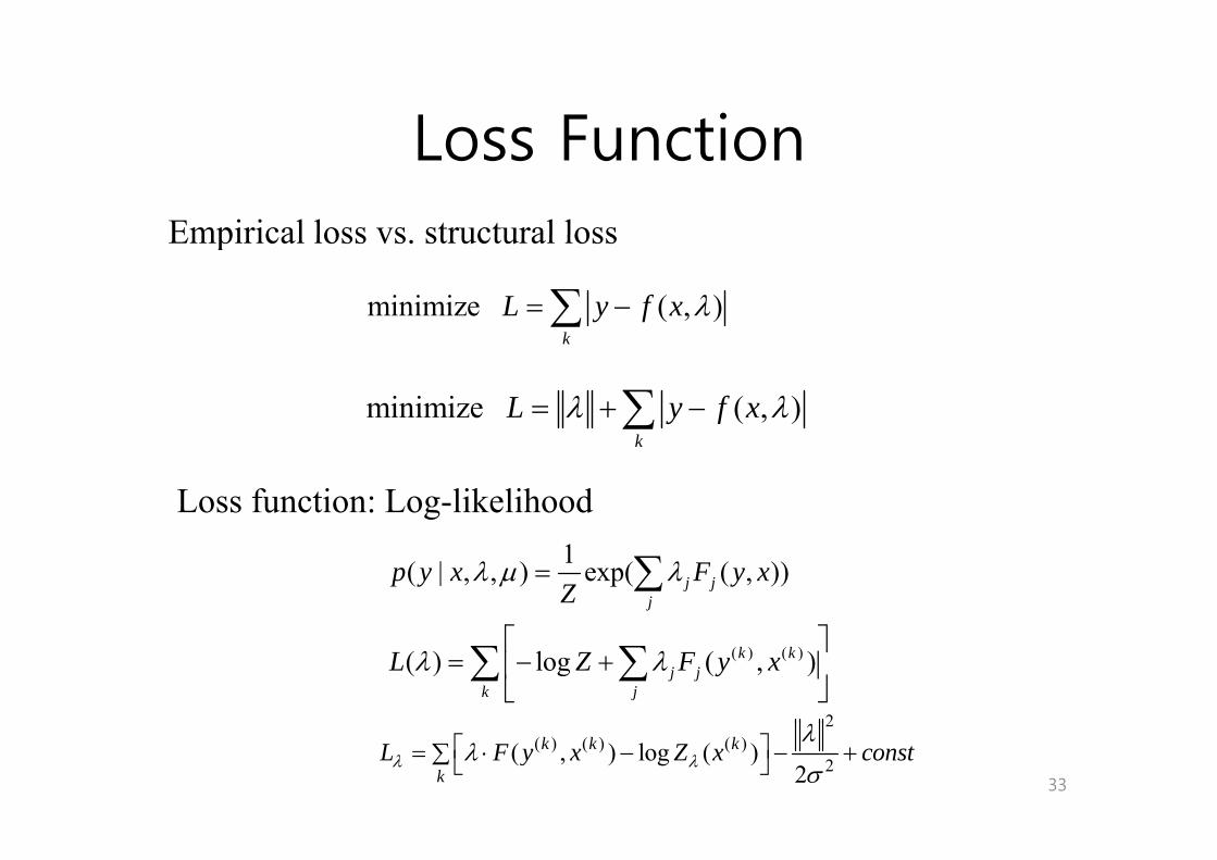
Loss FunctionLoss FunctionEmpirical loss vs structural lossEmpirical loss vs. structural loss

minimize ( , )k

L y f x λ= −∑k

minimize ( , )L y f xλ λ= + −∑

Loss function: Log-likelihood

k

1( | , , ) exp( ( , ))j jj

p y x F y xZ

λ μ λ=

⎡ ⎤

∑

( ) ( )( ) log ( , )k kj j

k j

L Z F y xλ λ⎡ ⎤

= − +⎢ ⎥⎣ ⎦

∑ ∑2

33

2( ) ( ) ( )

2( , ) log ( )2

k k k

kL F y x Z x constλ λ

λλ

σ⎡ ⎤= ⋅ − − +∑ ⎣ ⎦

Parameter EstimationParameter EstimationLog-likelihood ( ) '

( ) ( ) ( ( ))kk kL Z xλ λδ ⎡ ⎤

( ) ( )( ) log ( , )k kj j

k jL Z F y xλ λ

⎡ ⎤= − +⎢ ⎥

⎣ ⎦∑ ∑

( ) ( )( )

( ) ( )

( ( ))( , )

( )

( ) exp ( , )

k kj kkj

k k

L Z xF y x

Z x

Z x F y x

λ λ

λ

λ

δδλ

λ

⎡ ⎤= −∑ ⎢ ⎥

⎢ ⎥⎣ ⎦

= ⋅∑k j⎣ ⎦

( )( ) ( )( ) '

( ) ( )

exp( ( , )) ( , )( ( ))

y

k kjk

yk k

F y x F y xZ x

λ

λλ ⋅ ∗∑

=Differentiating the log-likelihood with

respect to parameter λj

Lδ

( ) ( )

( )

( ) exp ( , )

exp( ( )

k k

y

k

Z x F y x

F y x

λ λ

λ

⋅∑

⎛ ⎞⎜ ⎟⋅

( )( )

( , ) ( | , )[ ( , )] [ ( , )]k

kp Y X j jp Y x

kj

L E F Y X E F Y xλ

δδλ

= − ∑( )

( )( )

exp( ( , ) ) ( , )exp ( , )

(

kjky

y

F y x F y xF y x

λλ

⎜ ⎟⋅= ∗∑⎜ ⎟⋅∑⎜ ⎟

⎝ ⎠

( )( ) ( )| ) ( )k k∑By adding the model penalty it can be (p y= ( )( )

( ) ( )

( )( | )

| ) ( , )

( , )k

k kj

y

kjp Y x

x F y x

E F Y x

∗∑

=

By adding the model penalty, it can be rewritten as

( )( )

( , ) 2( | )[ ( , )] [ ( , )]k

kp Y X j jp Y x

L E F Y X E F Y xλ

δ λδλ

= − −∑

34

( , ) 2( | , )p Y X j jp Y xkj

λδλ σ∑

Optimizationp

⎡ ⎤( ) ( )( ) log ( , )k kj j

k jL Z F y xλ λ

⎡ ⎤= − +⎢ ⎥

⎣ ⎦∑ ∑

( )( )

( , ) ( | , )[ ( , )] [ ( , )]k

kp Y X j jp Y x

kj

L F Y X F Y xλ

δδλ

= − ∑E E

• Ep(y x) Fj(y,x) can be calculated easilyp(y,x) j(y, ) y• Ep(y|x) Fj(y,x) can be calculated by making use of a

forward-backward algorithmforward backward algorithm• Z can be estimated in the forward-backward algorithm

35

Calculating the ExpectationCalculating the Expectation

• First e define the transition matri of for position• First we define the transition matrix of y for position x as

1 1[ , ] exp ( , , , )i i i i iM y y f y y x iλ− −= ⋅

( ) ( )( ) ( | ) ( )k kE F Y F⎡ ⎤ ∑ ⎧( )( ) ( )

( | )

( ) ( )1 1

( , ) ( | ) ( , )

( , | ) ( , , )

kk k

j jp Y x y

n k ki i j i i

E F Y x p y x F y x

p y y x f y y x

λλ⎡ ⎤ = ∑⎣ ⎦

= ∑ ∑

01 0

1

i ii

TT

M i ni

M i n

αα

β

< ≤⎧= ⎨ =⎩

⎧ ≤ <⎪1

1 11 ,

1

( , | ) ( , , )

( )( )

i ii i j i i

i y y

Ti i i i i

p y y f y y

f M VZ

α β−

− −=

−

∑ ∑

∗ ∗= ∑

1 1 11

T i ii

M i ni n

ββ + +⎧ ≤ <⎪= ⎨=⎪⎩

T

1

1

( )

( ) ( ) 1

i

n Ti n

i

Z x

Z x M x

λ

λ α+⎡ ⎤= = ⋅∏⎢ ⎥⎣ ⎦

( ) 1( | )( )

Tk i i

ip y xZ xλ

α β−=

36

1i=⎣ ⎦All state features at position i

First order Numerical OptimizationFirst-order Numerical Optimization

Using Iterative Scaling (GIS, IIS)g g ( , )

• Initialize each λj (= 0 for example)j ( p )• Until convergence

- Solve for each parameter λj0Lδδλ

= p j

- Update each parameter using λj λj + ∆λj

jδλ

37

Second-order Numerical Optimization

2L L∂ ∂

Using newton optimization technique for the parameter estimation

2( 1) ( ) 1

2( )k k L Lλ λλλ

+ −∂ ∂= +

∂∂

Drawbacks: parameter value initializationAnd compute the second order (i.e. Hesse matrix), that is difficult

Solutions:- Conjugate-gradient (CG) (Shewchuk, 1994) - Limited-memory quasi-Newton (L-BFGS) (Nocedal and Wright, 1999) - Voted Perceptron (Colloins 2002)

38

Summary of CRFs

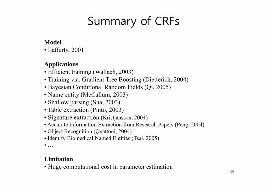
Model• Lafferty, 2001Lafferty, 2001

Applications• Efficient training (Wallach 2003)Efficient training (Wallach, 2003)• Training via. Gradient Tree Boosting (Dietterich, 2004)• Bayesian Conditional Random Fields (Qi, 2005)• Name entity (McCallum 2003)• Name entity (McCallum, 2003)• Shallow parsing (Sha, 2003)• Table extraction (Pinto, 2003)

Si i ( )• Signature extraction (Kristjansson, 2004)• Accurate Information Extraction from Research Papers (Peng, 2004)• Object Recognition (Quattoni, 2004)

Id tif Bi di l N d E titi (T i 2005)• Identify Biomedical Named Entities (Tsai, 2005)• …

Li it ti

39

Limitation• Huge computational cost in parameter estimation

HMM vs. CRF

( | )P Sφ

CRFHMM

arg max ( | )

arg max ( ) ( | )

P S

P P Sφ

φ

φ φ=( , )

arg max ( | )

1arg max f c S

P S

e

φ

λ

φ

∑=

( )1

arg max ( ) ( | )

arg max log ( | ) ( | )trans i i emit i i

P P S

P y y P s yφ

φ

φ φ

−

=

= ∑

arg max

arg max ( , )i ic i

eZ

f c Sφ

φλ

=

= ∑iyφ φ∈ ,c iφ

1. Both optimizations are over sums—this allows us to use any of the dynamic p y yprogramming HMM/GHMM decoding algorithms for fast, memory-efficient parsing, with the CRF scoring scheme used in place of the HMM/GHMM scoring scheme.

2 The CRF functions f (c S) may in fact be implemented using any type of sensor2. The CRF functions fi(c,S) may in fact be implemented using any type of sensor, including such probabilistic sensors as Markov chains, interpolated Markov models (IMM’s), decision trees, phylogenetic models, etc..., as well as any non-probabilistic sensor, such as n-mer counts or binary indicatorssuch as n-mer counts or binary indicators.

Appendix

A (di t l d) M k d fi ld (MRF) i 4 t l M ( X P G) h

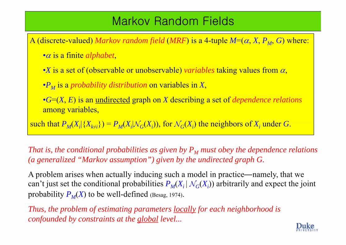
Markov Random FieldsMarkov Random Fields

A (discrete-valued) Markov random field (MRF) is a 4-tuple M=(α, X, PM, G) where:

•α is a finite alphabet,

•X is a set of (observable or unobservable) variables taking values from α,

•PM is a probability distribution on variables in X,

•G=(X, E) is an undirected graph on X describing a set of dependence relationsamong variables,

h th t P (X |{X }) P (X |N (X )) f N (X ) th i hb f X d Gsuch that PM(Xi|{Xk≠i}) = PM(Xi|NG(Xi)), for NG(Xi) the neighbors of Xi under G.

That is the conditional probabilities as given by P must obey the dependence relationsThat is, the conditional probabilities as given by PM must obey the dependence relations (a generalized “Markov assumption”) given by the undirected graph G.

A problem arises when actually inducing such a model in practice—namely, that we p y g p y,can’t just set the conditional probabilities PM(Xi | NG(Xi)) arbitrarily and expect the joint probability PM(X) to be well-defined (Besag, 1974).

h h bl f l ll f h hb h dThus, the problem of estimating parameters locally for each neighborhood is confounded by constraints at the global level...

Suppose P(x)>0 for all (joint) value assignments x to the variables in X Then by the

The Hammersley-Clifford TheoremThe Hammersley-Clifford Theorem

Suppose P(x)>0 for all (joint) value assignments x to the variables in X. Then by the Hammersley-Clifford theorem, the likelihood of x under model M is given by:

P (x) =1 eQ( x ) What is a clique?

PM (x) =

Ze

for normalization term Z:

Z = eQ( ′ x )∑

What is a clique?

where Q(x) has a unique expansion given by:

Z = e

′ x ∑

A clique is any subgraph in which all vertices are

Q(x0, x1,..., xn−1) = xiΦi (xi )∑ + xix jΦi, j (xi , xj )+ ...∑

Q( ) q p g yneighbors.

0≤i<n 0≤i< j<n

...+ x0x1...xn−1Φ0,1,...,n−1(x0, x1,..., xn−1)

d h Φ di l band where any Φi term not corresponding to a clique must be zero. (Besag, 1974)

The reason this is useful is that it provides a way to evaluate probabilities (whether joint or conditional) based on the “local” functions Φ.Thus, we can train an MRF by learning individual Φ functions—one for each clique.

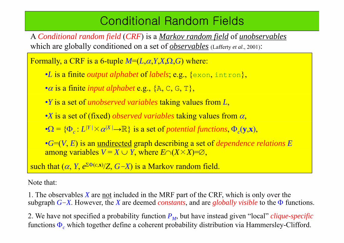
A Conditional random field (CRF) is a Markov random field of unobservables

Conditional Random FieldsConditional Random FieldsA Conditional random field (CRF) is a Markov random field of unobservableswhich are globally conditioned on a set of observables (Lafferty et al., 2001):

Formally, a CRF is a 6-tuple M=(L,α,Y,X,Ω,G) where:

•L is a finite output alphabet of labels; e.g., {exon, intron},

•α is a finite input alphabet e.g., {A, C, G, T},

•Y is a set of unobserved variables taking values from L,

•X is a set of (fixed) observed variables taking values from α,•Ω = {Φc : L|Y |×α|X |→ } is a set of potential functions, Φc(y,x),

•G=(V, E) is an undirected graph describing a set of dependence relations Ei bl h ( )among variables V = X ∪ Y, where E∩(X×X)=∅,

such that (α, Y, eΣΦ(c,x)/Z, G-X) is a Markov random field.

Note that:

1. The observables X are not included in the MRF part of the CRF, which is only over the subgraph G-X. However, the X are deemed constants, and are globally visible to the Φ functions.subgraph G X. However, the X are deemed constants, and are globally visible to the Φ functions.

2. We have not specified a probability function PM, but have instead given “local” clique-specificfunctions Φc which together define a coherent probability distribution via Hammersley-Clifford.

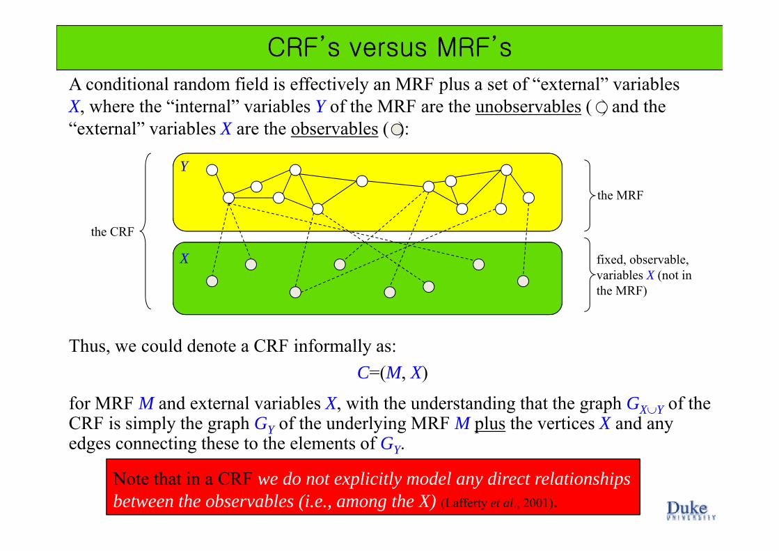
A conditional random field is effectively an MRF plus a set of “external” variables

CRF’s versus MRF’sCRF’s versus MRF’s

A conditional random field is effectively an MRF plus a set of external variables X, where the “internal” variables Y of the MRF are the unobservables ( ) and the “external” variables X are the observables ( ):

the MRF

Y

fixed, observable, variables X (not in

the CRF

Xvariables X (not in the MRF)

Thus, we could denote a CRF informally as: C=(M, X)

for MRF M and e ternal ariables X ith the nderstanding that the graph G of thefor MRF M and external variables X, with the understanding that the graph GX∪Y of the CRF is simply the graph GY of the underlying MRF M plus the vertices X and any edges connecting these to the elements of GY.

Note that in a CRF we do not explicitly model any direct relationships between the observables (i.e., among the X) (Lafferty et al., 2001).