Chapter 8 A Genetic Programming Tutorial - PBworksphil415.pbworks.com/f/JKTutorial.pdf · Chapter 8 Chapter 8 A Genetic Programming Tutorial John 1R. Koza and Riccardo Poli2 1 St

Chapter 8

Chapter 8

A Genetic Programming Tutorial

John R. Koza1 and Riccardo Poli2

1Stanford University, Stanford, California 2Department of Computer Science, University of Essex, UK

Abstract: Genetic programming is a technique to automatically discover computer programs using principles of Darwinian evolution. This chapter introduces the basics of genetic programming. To make the material more suitable for beginners, these are illustrated with an extensive example. In addition, the chapter touches upon some of the more advanced variants of genetic programming as well as its theoretical foundations. Numerous pointers to further reading, software tools and Web sites are also provided.

Key words: Genetic programming, genetic algorithms, human-competitive machine intelligence, machine learning, schema theory

1. INTRODUCTION

The goal of getting computers to automatically solve problems is central to artificial intelligence, machine learning, and the broad area encompassed by what Turing called “machine intell igence” (Turing 1948, 1950).

In his 1983 talk entitled “AI: Where It Has Been and Where It Is Going, machine learning pioneer Arthur Samuel stated the main goal of the fields of machine learning and artificial intelligence:

“ [T]he aim [is] … to get machines to exhibit behavior, which if done by humans, would be assumed to involve the use of intelligence.”

Genetic programming is a systematic method for getting computers to automatically solve a problem starting from a high-level statement of what needs to be done. Genetic programming is a domain-independent method that genetically breeds a population of computer programs to solve a problem. Specifically, genetic programming iteratively transforms a population of computer programs into a new generation of programs by

Chapter 8

applying analogs of naturally occurring genetic operations. This process is i llustrated in Figure 1.

Figure 1. Main loop of genetic programming

The genetic operations include crossover (sexual recombination), mutation, reproduction, gene duplication, and gene deletion. Analogs of developmental processes are sometimes used to transform an embryo into a fully developed structure. Genetic programming is an extension of the genetic algorithm (Holland 1975) in which the structures in the population are not fixed-length character strings that encode candidate solutions to a problem, but programs that, when executed, are the candidate solutions to the problem.

Programs are expressed in genetic programming as syntax trees rather than as lines of code. For example, the simple expression max(x*x,x+3*y)is represented as shown in Figure 2. The tree includes nodes (which we will also call point) and l inks. The nodes indicate the instructions to execute. The links indicate the arguments for each instruction. In the following the internal nodes in a tree will be called functions, while the tree’s leaves will be called terminals.

Figure 2. Basic tree-like program representation used in genetic programming

Chapter 8

Figure 3. Multi-tree program representation

In more advanced forms of genetic programming, programs can be composed of multiple components (e.g., subroutines). In this case the representation used in genetic programming is a set of trees (one for each component) grouped together under a special node called root, as i llustrated in Figure 3. We will call these (sub)trees branches. The number and type of the branches in a program, together with certain other features of the structure of the branches, form the architecture of the program.

Genetic programming trees and their corresponding expressions can equivalently be represented in prefix notation (e.g., as Lisp S-expressions). In prefix notation, functions always precede their arguments. For example, max(x*x,x+3*y) becomes (max (* x x)(+ x (* 3 y))). In this notation, it is easy to see the correspondence between expressions and their syntax trees. Simple recursive procedures can convert prefix-notation expressions into infix-notation expressions and vice versa. Therefore, in the following, we will use trees and their corresponding prefix-notation expressions interchangeably.

2. PREPARATORY STEPS OF GENETIC PROGRAMMING

Genetic programming starts from a high-level statement of the requirements of a problem and attempts to produce a computer program that solves the problem.

Chapter 8

The human user communicates the high-level statement of the problem to the genetic programming algorithm by performing certain well-defined preparatory steps.

The five major preparatory steps for the basic version of genetic programming require the human user to specify 1. the set of terminals (e.g., the independent variables of the problem, zero-

argument functions, and random constants) for each branch of the to-be-evolved program,

2. the set of primitive functions for each branch of the to-be-evolved program,

3. the fitness measure (for explicitly or implicitly measuring the fitness of individuals in the population),

4. certain parameters for controlling the run, and 5. the termination criterion and method for designating the result of the run.

The first two preparatory steps specify the ingredients that are available to create the computer programs. A run of genetic programming is a competitive search among a diverse population of programs composed of the available functions and terminals.

The identification of the function set and terminal set for a particular problem (or category of problems) is usually a straightforward process. For some problems, the function set may consist of merely the arithmetic functions of addition, subtraction, multiplication, and division as well as a conditional branching operator. The terminal set may consist of the program’s external inputs (independent variables) and numerical constants.

For many other problems, the ingredients include specialized functions and terminals. For example, if the goal is to get genetic programming to automatically program a robot to mop the entire floor of an obstacle-laden room, the human user must tell genetic programming what the robot is capable of doing. For example, the robot may be capable of executing functions such as moving, turning, and swishing the mop.

If the goal is the automatic creation of a controller, the function set may consist of integrators, differentiators, leads, lags, gains, adders, subtractors, and the like and the terminal set may consist of signals such as the reference signal and plant output.

If the goal is the automatic synthesis of an analog electrical circuit, the function set may enable genetic programming to construct circuits from components such as transistors, capacitors, and resistors. Once the human user has identified the primitive ingredients for a problem of circuit synthesis, the same function set can be used to automaticall y synthesize an amplifier, computational circuit, active filter, voltage reference circuit, or any other circuit composed of these ingredients.

Chapter 8

The third preparatory step concerns the fitness measure for the problem. The fitness measure speci fies what needs to be done. The fitness measure is the primary mechanism for communicating the high-level statement of the problem’s requirements to the genetic programming system. For example, if the goal is to get genetic programming to automatically synthesize an amplifier, the fitness function is the mechanism for telling genetic programming to synthesize a circuit that amplifies an incoming signal (as opposed to, say, a circuit that suppresses the low frequencies of an incoming signal or that computes the square root of the incoming signal). The first two preparatory steps define the search space whereas the fitness measure implicitly specifies the search’s desired goal.

The fourth and fifth preparatory steps are administrative. The fourth preparatory step entails specifying the control parameters for the run. The most important control parameter is the population size. Other control parameters include the probabilities of performing the genetic operations, the maximum size for programs, and other details of the run.

The fifth preparatory step consists of specifying the termination criterion and the method of designating the result of the run. The termination criterion may include a maximum number of generations to be run as well as a problem-speci fic success predicate. The single best-so-far individual is then harvested and designated as the result of the run.

3. EXECUTIONAL STEPS OF GENETIC PROGRAMMING

After the user has performed the preparatory steps for a problem, the run of genetic programming can be launched. Once the run is launched, a series of well-defined, problem-independent steps is executed.

Genetic programming typically starts with a population of randomly generated computer programs composed of the available programmatic ingredients (as provided by the human user in the first and second preparatory steps).

Genetic programming iteratively transforms a population of computer programs into a new generation of the population by applying analogs of naturally occurring genetic operations. These operations are applied to individual(s) selected from the population. The individuals are probabilistically selected to participate in the genetic operations based on their fitness (as measured by the fitness measure provided by the human user in the third preparatory step). The iterative transformation of the population is executed inside the main generational loop of the run of genetic programming.

Chapter 8

The executional steps of genetic programming are as follows: 1. Randomly create an initial population (generation 0) of individual

computer programs composed of the available functions and terminals. 2. Iteratively perform the following sub-steps (called a generation) on the

population until the termination criterion is satisfied: a) Execute each program in the population and ascertain its fitness

(explicitly or implicitly) using the problem’s fitness measure. b) Select one or two individual program(s) from the population with a

probability based on fitness (with reselection allowed) to participate in the genetic operations in (c).

c) Create new individual program(s) for the population by applying the following genetic operations with specified probabilities: – Reproduction: Copy the selected individual program to the new

population. – Crossover: Create new offspring program(s) for the new

population by recombining randomly chosen parts from two selected programs.

– Mutation: Create one new offspring program for the new population by randomly mutating a randomly chosen part of one selected program.

– Architecture-altering operations: Choose an architecture-altering operation from the available repertoire of such operations and create one new offspring program for the new population by applying the chosen architecture-altering operation to one selected program.

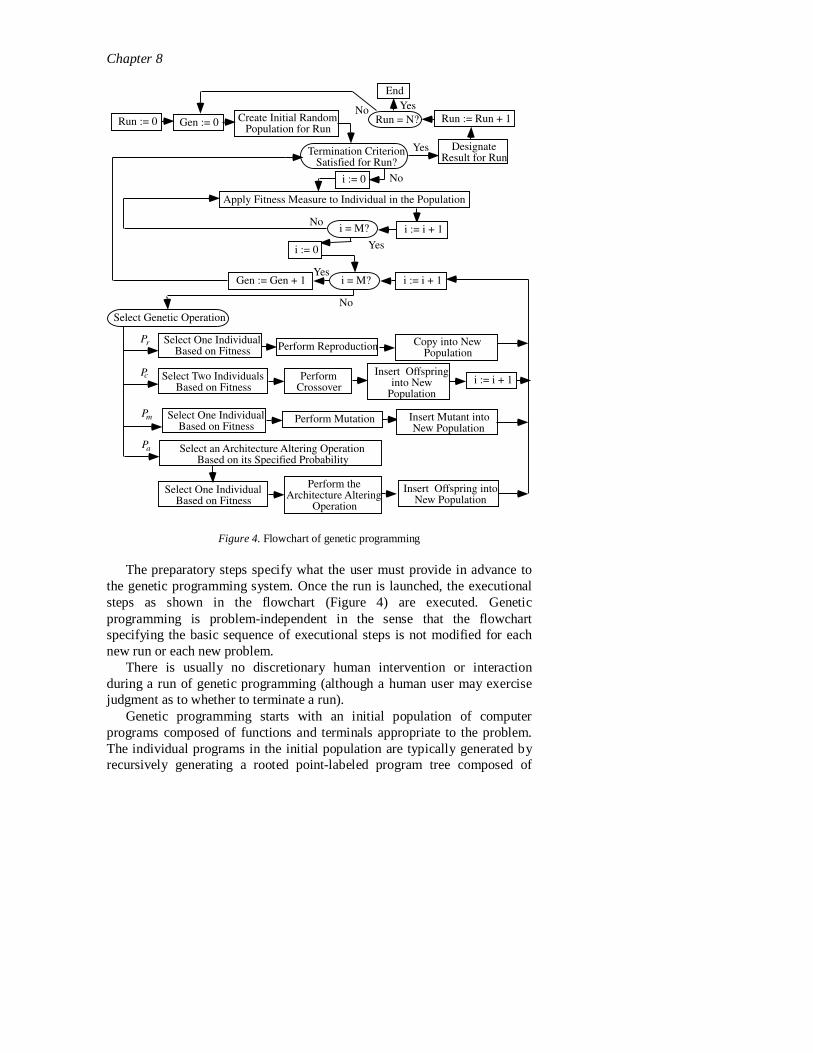
3. After the termination criterion is satisfied, the single best program in the population produced during the run (the best-so-far individual) is harvested and designated as the result of the run. If the run is successful, the result may be a solution (or approximate solution) to the problem. Figure 4 is a flowchart of genetic programming showing the genetic

operations of crossover, reproduction, and mutation as well as the architecture-altering operations. This flowchart shows a two-offspring version of the crossover operation.

Chapter 8

Perform Reproduction

Yes

No

Gen := Gen + 1

Select Two IndividualsBased on Fitness

PerformCrossover

Perform Mutation Insert Mutant intoNew Population

Copy into NewPopulation

i := i + 1

Select One IndividualBased on Fitness

Pr

Pc

Pm

Select Genetic Operation

i = M?

Create Initial RandomPopulation for Run

No

Termination CriterionSatisfied for Run?

Yes

Gen := 0 Run := Run + 1

DesignateResult for Run

End

Run := 0

i := 0

NoRun = N?

Yes

i := 0

i := i + 1i = M?

Apply Fitness Measure to Individual in the Population

Yes

No


Insert Offspringinto New

Populationi := i + 1

Select an Architecture Altering OperationBased on its Specified Probability

Perform theArchitecture Altering

Operation

Insert Offspring intoNew Population


Pa

Figure 4. Flowchart of genetic programming

The preparatory steps speci fy what the user must provide in advance to the genetic programming system. Once the run is launched, the executional steps as shown in the flowchart (Figure 4) are executed. Genetic programming is problem-independent in the sense that the flowchart specifying the basic sequence of executional steps is not modified for each new run or each new problem.

There is usually no discretionary human intervention or interaction during a run of genetic programming (although a human user may exercise judgment as to whether to terminate a run).

Genetic programming starts with an initial population of computer programs composed of functions and terminals appropriate to the problem. The individual programs in the initial population are typically generated by recursively generating a rooted point-labeled program tree composed of

Chapter 8

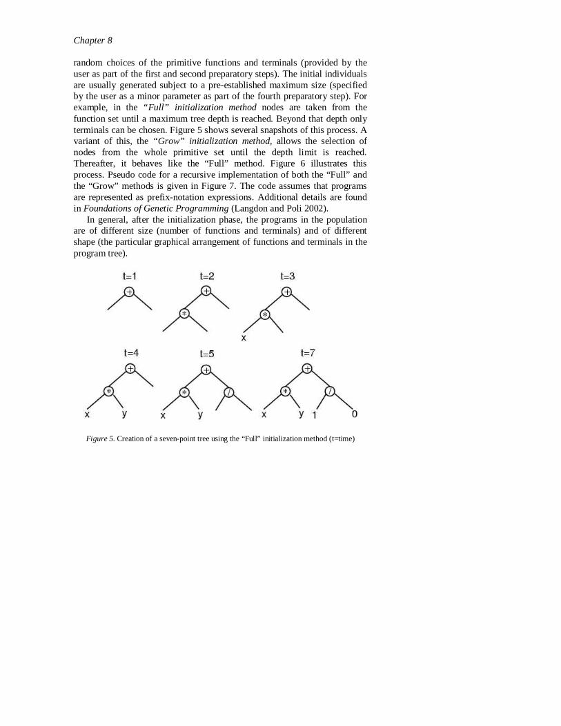
random choices of the primitive functions and terminals (provided by the user as part of the first and second preparatory steps). The initial individuals are usually generated subject to a pre-established maximum size (speci fied by the user as a minor parameter as part of the fourth preparatory step). For example, in the “ Full” initialization method nodes are taken from the function set until a maximum tree depth is reached. Beyond that depth only terminals can be chosen. Figure 5 shows several snapshots of this process. A variant of this, the “ Grow” initialization method, allows the selection of nodes from the whole primitive set until the depth limit is reached. Thereafter, it behaves like the “Full” method. Figure 6 illustrates this process. Pseudo code for a recursive implementation of both the “Full” and the “Grow” methods is given in Figure 7. The code assumes that programs are represented as prefix-notation expressions. Additional details are found in Foundations of Genetic Programming (Langdon and Poli 2002).

In general, after the initialization phase, the programs in the population are of different size (number of functions and terminals) and of different shape (the particular graphical arrangement of functions and terminals in the program tree).

Figure 5. Creation of a seven-point tree using the “Full” initialization method (t=time)

Chapter 8

Figure 6. Creation of a f ive-point tree using the “Grow” initialization method (t=time)

Figure 7. Pseudo code for recursive program generation with the “Full” and “Grow” methods

Each individual program in the population is either measured or compared in terms of how well it performs the task at hand (using the fitness measure provided in the third preparatory step). For many problems, this measurement yields a single explicit numerical value, called fitness. Normally, fitness evaluation requires executing the programs in the population, often multiple times, within the genetic programming system. A variety of execution strategies exist, including the (relatively uncommon)

Chapter 8

off-l ine or on-line compilation and linking and the (relatively common) virtual-machine-code compilation and interpretation.

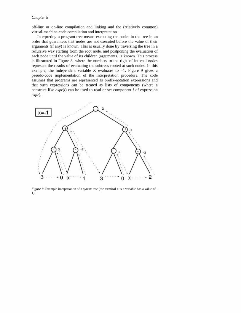
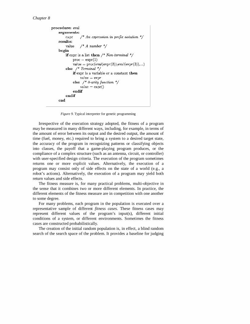
Interpreting a program tree means executing the nodes in the tree in an order that guarantees that nodes are not executed before the value of their arguments (if any) is known. This is usually done by traversing the tree in a recursive way starting from the root node, and postponing the evaluation of each node until the value of its children (arguments) is known. This process is i llustrated in Figure 8, where the numbers to the right of internal nodes represent the results of evaluating the subtrees rooted at such nodes. In this example, the independent variable X evaluates to –1. Figure 9 gives a pseudo-code implementation of the interpretation procedure. The code assumes that programs are represented as prefix-notation expressions and that such expressions can be treated as lists of components (where a construct l ike expr(i) can be used to read or set component i of expression expr).

Figure 8. Example interpretation of a syntax tree (the terminal x is a variable has a value of -1)

Chapter 8

Figure 9. Typical interpreter for genetic programming

Irrespective of the execution strategy adopted, the fitness of a program may be measured in many di fferent ways, including, for example, in terms of the amount of error between its output and the desired output, the amount of time (fuel, money, etc.) required to bring a system to a desired target state, the accuracy of the program in recognizing patterns or classifying objects into classes, the payoff that a game-playing program produces, or the compliance of a complex structure (such as an antenna, circuit, or controller) with user-speci fied design criteria. The execution of the program sometimes returns one or more explicit values. Alternatively, the execution of a program may consist only of side effects on the state of a world (e.g., a robot’s actions). Alternatively, the execution of a program may yield both return values and side effects.

The fitness measure is, for many practical problems, multi-objective in the sense that it combines two or more different elements. In practice, the different elements of the fitness measure are in competition with one another to some degree.

For many problems, each program in the population is executed over a representative sample of different fitness cases. These fitness cases may represent different values of the program’s input(s), different initial conditions of a system, or different environments. Sometimes the fitness cases are constructed probabilistically.

The creation of the initial random population is, in effect, a blind random search of the search space of the problem. It provides a baseline for judging

Chapter 8

future search efforts. Typically, the individual programs in generation 0 all have exceedingly poor fitness. Nonetheless, some individuals in the population are (usually) more fit than others. The differences in fitness are then exploited by genetic programming. Genetic programming applies Darwinian selection and the genetic operations to create a new population of offspring programs from the current population.

The genetic operations include crossover (sexual recombination), mutation, reproduction, and the architecture-altering operations. Given copies of two parent trees, typically, crossover involves randomly selecting a crossover point (which can equivalently be thought of as either a node or a l ink between nodes) in each parent tree and swapping the sub-trees rooted at the crossover points, as exemplified in Figure 10. Often crossover points are not selected with uniform probability. A frequent strategy is, for example, to select internal nodes (functions) 90% of the times, and any node for the remaining 10% of the times. Traditional mutation consists of randomly selecting a mutation point in a tree and substituting the sub-tree rooted there with a randomly generated sub-tree, as illustrated in Figure 11. Mutation is sometimes implemented as crossover between a program and a newly generated random program (this is also known as “ headless chicken” crossover). Reproduction involves simply copying certain individuals into the new population. Architecture altering operations will be discussed later in this chapter.

Figure 10. Example of two-child crossover between syntax trees

Chapter 8

Figure 11. Example of sub-tree mutation

The genetic operations described above are applied to individual(s) that are probabilistically selected from the population based on fitness. In this probabilistic selection process, better individuals are favored over inferior individuals. However, the best individual in the population is not necessaril y selected and the worst individual in the population is not necessarily passed over.

After the genetic operations are performed on the current population, the population of offspring (i.e., the new generation) replaces the current population (i.e., the now-old generation). This iterative process of measuring fitness and performing the genetic operations is repeated over many generations.

The run of genetic programming terminates when the termination criterion (as provided by the fifth preparatory step) is satisfied. The outcome of the run is specified by the method of result designation. The best individual ever encountered during the run (i.e., the best-so-far individual) is typically designated as the result of the run.

All programs in the initial random population (generation 0) of a run of genetic programming are syntactically valid, executable programs. The genetic operations that are performed during the run (i.e., crossover, mutation, reproduction, and the architecture-altering operations) are designed to produce offspring that are syntactically valid, executable programs. Thus, every individual created during a run of genetic programming (including, in particular, the best-of-run individual) is a syntactically valid, executable program.

There are numerous alternative implementations of genetic programming that vary from the preceding brief description.

Chapter 8

4. EXAMPLE OF A RUN OF GENETIC PROGRAMMING

To provide concreteness, this section contains an il lustrative run of genetic programming in which the goal is to automatically create a computer program whose output is equal to the values of the quadratic polynomial x2+x+1 in the range from –1 to +1. That is, the goal is to automatically create a computer program that matches certain numerical data. This process is sometimes called system identification or symbolic regression.

We begin with the five preparatory steps. The purpose of the first two preparatory steps is to specify the ingredients

of the to-be-evolved program. Because the problem is to find a mathematical function of one

independent variable, the terminal set (inputs to the to-be-evolved program) includes the independent variable, x. The terminal set also includes numerical constants. That is, the terminal set, T, is

T = {X, ℜ} . Here ℜ denotes constant numerical terminals in some reasonable range

(say from –5.0 to +5.0). The preceding statement of the problem is somewhat flexible in that it

does not specify what functions may be employed in the to-be-evolved program. One possible choice for the function set consists of the four ordinary arithmetic functions of addition, subtraction, multiplication, and division. This choice is reasonable because mathematical expressions typically include these functions. Thus, the function set, F, for this problem is

F = {+, -, *, %} . The two-argument +, -, *, and % functions add, subtract, multiply, and

divide, respectively. To avoid run-time errors, the division function % is protected: it returns a value of 1 when division by 0 is attempted (including 0 divided by 0), but otherwise returns the quotient of its two arguments.

Each individual in the population is a composition of functions from the specified function set and terminals from the specified terminal set.

The third preparatory step involves constructing the fitness measure. The purpose of the fitness measure is to specify what the human wants. The high-level goal of this problem is to find a program whose output is equal to the values of the quadratic polynomial x2+x+1. Therefore, the fitness assigned to a particular individual in the population for this problem must reflect how closely the output of an individual program comes to the target polynomial x2+x+1. The fitness measure could be defined as the value of the integral (taken over values of the independent variable x between –1.0 and +1.0) of the absolute value of the di fferences (errors) between the value of the

Chapter 8

individual mathematical expression and the target quadratic polynomial x2+x+1. A smaller value of fitness (error) is better. A fitness (error) of zero would indicate a perfect fit.

For most problems of symbolic regression or system identi fication, it is not practical or possible to analytically compute the value of the integral of the absolute error. Thus, in practice, the integral is numerically approximated using dozens or hundreds of different values of the independent variable x in the range between –1.0 and +1.0.

The population size in this small illustrative example will be just four. In actual practice, the population size for a run of genetic programming consists of thousands or millions of individuals. In actual practice, the crossover operation is commonly performed on about 90% of the individuals in the population; the reproduction operation is performed on about 8% of the population; the mutation operation is performed on about 1% of the population; and the architecture-altering operations are performed on perhaps 1% of the population. Because this illustrative example involves an abnormally small population of only four individuals, the crossover operation will be performed on two individuals and the mutation and reproduction operations will each be performed on one individual. For simplicity, the architecture-altering operations are not used for this problem.

A reasonable termination criterion for this problem is that the run will continue from generation to generation until the fitness of some individual gets below 0.01. In this contrived example, the run will (atypically) yield an algebraically perfect solution (for which the fitness measure attains the ideal value of zero) after merely one generation.

Now that we have performed the five preparatory steps, the run of genetic programming can be launched. That is, the executional steps shown in the flowchart of Figure 4 are now performed.

Genetic programming starts by randomly creating a population of four individual computer programs. The four programs are shown in Figure 12 in the form of trees.

The first randomly constructed program tree (Figure 12a) is equivalent to the mathematical expression x+1. A program tree is executed in a depth-first way, from left to right, in the style of the LISP programming language. Specificall y, the addition function (+) is executed with the variable x and the constant value 1 as its two arguments. Then, the two-argument subtraction function (–) is executed. Its first argument is the value returned by the just-executed addition function. Its second argument is the constant value 0. The overall result of executing the entire program tree is thus x+1.

The first program (Figure 12a) was constructed, using the “Grow” method, by first choosing the subtraction function for the root (top point) of the program tree. The random construction process continued in a depth-first

Chapter 8

fashion (from left to right) and chose the addition function to be the first argument of the subtraction function. The random construction process then chose the terminal x to be the first argument of the addition function (thereby terminating the growth of this path in the program tree). The random construction process then chose the constant terminal 1 as the second argument of the addition function (thereby terminating the growth along this path). Finally, the random construction process chose the constant terminal 0 as the second argument of the subtraction function (thereby terminating the entire construction process).

+

x 1

-

0

+

2 0*

x

1

+

x

x

*

-

-1 -2

(a) (b) (c) (d)

+1x 2 +1x 2 x

Figure 12. Initial population of four randomly created individuals of generation 0

� �

�

� � ��

�

� � ��

�

� � �

� ��

Figure 13. The fitness of each of the four randomly created individuals of generation 0 is equal to the area between two curves.

Chapter 8

+

x 1

-

0 x

-

0

+

1

1 *

x+

x

% 0

+

x x

(a) (b) (c) (d)

+1x 1 x 2 + +1x x

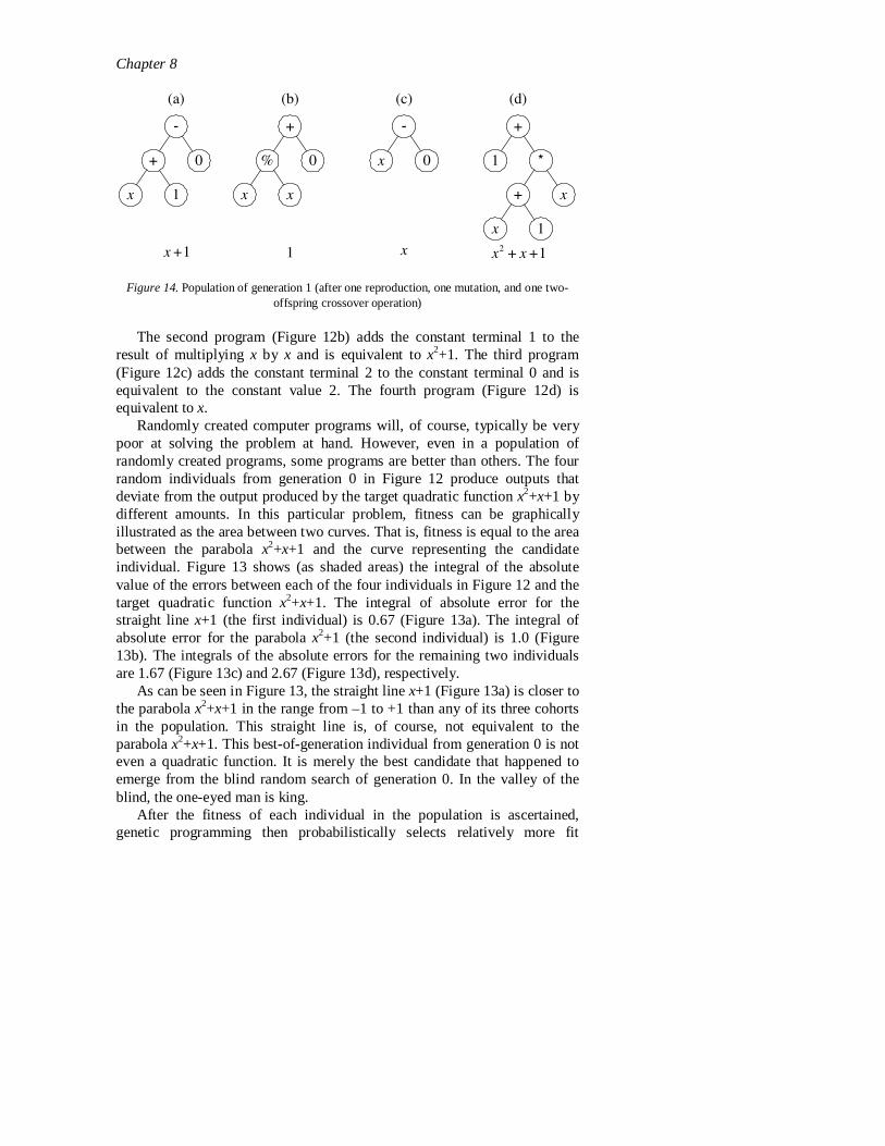
Figure 14. Population of generation 1 (after one reproduction, one mutation, and one two-offspring crossover operation)

The second program (Figure 12b) adds the constant terminal 1 to the result of multiplying x by x and is equivalent to x2+1. The third program (Figure 12c) adds the constant terminal 2 to the constant terminal 0 and is equivalent to the constant value 2. The fourth program (Figure 12d) is equivalent to x.

Randomly created computer programs will, of course, typically be very poor at solving the problem at hand. However, even in a population of randomly created programs, some programs are better than others. The four random individuals from generation 0 in Figure 12 produce outputs that deviate from the output produced by the target quadratic function x2+x+1 by different amounts. In this particular problem, fitness can be graphicall y i llustrated as the area between two curves. That is, fitness is equal to the area between the parabola x2+x+1 and the curve representing the candidate individual. Figure 13 shows (as shaded areas) the integral of the absolute value of the errors between each of the four individuals in Figure 12 and the target quadratic function x2+x+1. The integral of absolute error for the straight line x+1 (the first individual) is 0.67 (Figure 13a). The integral of absolute error for the parabola x2+1 (the second individual) is 1.0 (Figure 13b). The integrals of the absolute errors for the remaining two individuals are 1.67 (Figure 13c) and 2.67 (Figure 13d), respectively.

As can be seen in Figure 13, the straight l ine x+1 (Figure 13a) is closer to the parabola x2+x+1 in the range from –1 to +1 than any of its three cohorts in the population. This straight l ine is, of course, not equivalent to the parabola x2+x+1. This best-of-generation individual from generation 0 is not even a quadratic function. It is merely the best candidate that happened to emerge from the blind random search of generation 0. In the valley of the blind, the one-eyed man is king.

After the fitness of each individual in the population is ascertained, genetic programming then probabilistically selects relatively more fit

Chapter 8

programs from the population. The genetic operations are applied to the selected individuals to create offspring programs. The most commonly employed methods for selecting individuals to participate in the genetic operations are tournament selection and fitness-proportionate selection. In both methods, the emphasis is on selecting relatively fit individuals. An important feature common to both methods is that the selection is not greedy. Individuals that are known to be inferior will be selected to a certain degree. The best individual in the population is not guaranteed to be selected. Moreover, the worst individual in the population will not necessarily be excluded. Anything can happen and nothing is guaranteed.

We first perform the reproduction operation. Because the first individual (Figure 12a) is the most fit individual in the population, it is very likely to be selected to participate in a genetic operation. Let’s suppose that this particular individual is, in fact, selected for reproduction. If so, it is copied, without alteration, into the next generation (generation 1). It is shown in Figure 14a as part of the population of the new generation.

We next perform the mutation operation. Because selection is probabilistic, it is possible that the third best individual in the population (Figure 12c) is selected. One of the three nodes of this individual is then randomly picked as the site for the mutation. In this example, the constant terminal 2 is picked as the mutation site. This program is then randomly mutated by deleting the entire subtree rooted at the picked point (in this case, just the constant terminal 2) and inserting a subtree that is randomly grown in the same way that the individuals of the initial random population were originally created. In this particular instance, the randomly grown subtree computes the quotient of x and x using the protected division operation %. The resulting individual is shown in Figure 14b. This particular mutation changes the original individual from one having a constant value of 2 into one having a constant value of 1. This particular mutation improves fitness from 1.67 to 1.00.

Finally, we perform the crossover operation. Because the first and second individuals in generation 0 are both relatively fit, they are likely to be selected to participate in crossover. The selection (and reselection) of relatively more fit individuals and the exclusion and extinction of unfit individuals is a characteristic feature of Darwinian selection. The first and second programs are mated sexually to produce two offspring (using the two-offspring version of the crossover operation). One point of the first parent (Figure 12a), namely the + function, is randomly picked as the crossover point for the first parent. One point of the second parent (Figure 12b), namely its leftmost terminal x, is randomly picked as the crossover point for the second parent. The crossover operation is then performed on the two parents. The two offspring are shown in Figures 2.4c and 2.4d. One of

Chapter 8

the offspring (Figure 14c) is equivalent to x and is not noteworthy. However, the other offspring (Figure 14d) is equivalent to x2+x+1 and has a fitness (integral of absolute errors) of zero. Because the fitness of this individual is below 0.01, the termination criterion for the run is satisfied and the run is automatically terminated. This best-so-far individual (Figure 14d) is designated as the result of the run. This individual is an algebraically correct solution to the problem.

Note that the best-of-run individual (Figure 14d) incorporates a good trait (the quadratic term x2) from the second parent (Figure 12b) with two other good traits (the linear term x and constant term of 1) from the first parent (Figure 12a). The crossover operation produced a solution to this problem by recombining good traits from these two relatively fit parents into a superior (indeed, perfect) offspring.

In summary, genetic programming has, in this example, automatically created a computer program whose output is equal to the values of the quadratic polynomial x2+x+1 in the range from –1 to +1.

5. ADVANCED FEATURES OF GENETIC PROGRAMMING

Various advanced features of genetic programming are not covered by the foregoing illustrative problem and the foregoing discussion of the preparatory and executional steps of genetic programming.

5.1 Constrained Syntactic Structures

For certain simple problems (such as the illustrative problem above), the search space for a run of genetic programming consists of the unrestricted set of possible compositions of the problem’s functions and terminals.

However, for many problems, a constrained syntactic structure imposes restrictions on how the functions and terminals may be combined.

Consider, for example, a function that instructs a robot to turn by a certain angle. In a typical implementation of this hypothetical function, the function’s first argument may be required to return a numerical value (representing the desired turning angle) and its second argument may be required to be a follow-up command (e.g., move, turn, stop). In other words, the functions and terminals permitted in the two argument subtrees for this particular function are restricted. These restrictions are implemented by means of syntactic rules of construction.

Chapter 8

A constrained syntactic structure (sometimes called strong typing) is a grammar that specifies the functions or terminals that are permitted to appear as a specified argument of a specified function in the program tree.

When a constrained syntactic structure is used, there are typically multiple function sets and multiple terminal sets. The rules of construction specify where the different function sets or terminal sets may be used.

When a constrained syntactic structure is used, all the individuals in the initial random population (generation 0) are created so as to comply with the constrained syntactic structure. All genetic operations (i.e., crossover, mutation, reproduction, and the architecture-altering operations) that are performed during the run are designed to produce offspring that comply with the requirements of the constrained syntactic structure. Thus, all individuals (including, in particular, the best-of-run individual) that are produced during the run of genetic programming will necessarily comply with the requirements of the constrained syntactic structure.

5.2 Automatically Defined Functions

Human computer programmers organize sequences of reusable steps into subroutines. They then repeatedly invoke the subroutines—typically with different instantiations of the subroutine’s dummy variables (formal parameters). Reuse eliminates the need to “reinvent the wheel” on each occasion when a particular sequence of steps may be useful. Reuse makes it possible to exploit a problem’s modularities, symmetries, and regularities (and thereby potentially accelerate the problem-solving process).

Programmers commonly organize their subroutines into hierarchies. The automatically defined function (ADF) is one of the mechanisms by

which genetic programming implements the parameterized reuse and hierarchical invocation of evolved code. Each automatically defined function resides in a separate function-defining branch within the overall multi-part computer program (see Figure 3). When automatically defined functions are being used, a program consists of one (or more) function-defining branches (i.e., automatically defined functions) as well as one or more main result-producing branches. An automatically defined function may possess zero, one, or more dummy variables (formal parameters). The body of an automatically defined function contains its work-performing steps. Each automatically defined function belongs to a particular program in the population. An automatically defined function may be called by the program’s main result-producing branch, another automatically defined function, or another type of branch (such as those described below). Recursion is sometimes allowed. Typically, the automatically defined functions are invoked with different instantiations of their dummy variables.

Chapter 8

The work-performing steps of the program’s main result-producing branch and the work-performing steps of each automatically defined function are automatically and simultaneously created during the run of genetic programming.

The program’s main result-producing branch and its automaticall y defined functions typically have different function and terminal sets. A constrained syntactic structure is used to implement automatically defined functions.

Automatically defined functions are the focus of Genetic Programming II: Automatic Discovery of Reusable Programs (Koza 1994a) and the videotape Genetic Programming II Videotape: The Next Generation (Koza 1994b).

5.3 Automatically Defined Iterations, Automatically Defined Loops, Automatically Defined Recursions, and Automatically Defined Stores

Automatically defined iterations (ADIs), automatically defined loops (ADLs), and automatically defined recursions (ADRs) provide means (in addition to automatically defined functions) to reuse code.

Automatically defined stores (ADSs) provide means to reuse the result of executing code.

Automatically defined iterations, automatically defined loops, automatically defined recursions, and automatically defined stores are described in Genetic Programming III: Darwinian Invention and Problem Solving (Koza, Bennett, Andre, and Keane 1999).

5.4 Program Architecture and Architecture-Altering Operations

The architecture of a program consists of – the total number of branches, – the type of each branch (e.g., result-producing branch, automatically

defined function, automatically defined iteration, automatically defined loop, automatically defined recursion, or automatically defined store),

– the number of arguments (if any) possessed by each branch, and – if there is more than one branch, the nature of the hierarchical references

(if any) allowed among the branches. There are three ways by which genetic programming can arrive at the

architecture of the to-be-evolved computer program: – The human user may prespeci fy the architecture of the overall program

(i.e., perform an additional architecture-defining preparatory step). That

Chapter 8

is, the number of preparatory steps is increased from the five previously itemized to six.

– The run may employ evolutionary selection of the architecture (as described in Genetic Programming II), thereby enabling the architecture of the overall program to emerge from a competitive process during the run of genetic programming. When this approach is used, the number of preparatory steps remains at the five previously itemized.

– The run may employ the architecture-altering operations (Koza 1994c, 1995; Koza, Bennett, Andre, and Keane 1999), thereby enabling genetic programming to automatically create the architecture of the overall program dynamically during the run. When this approach is used, the number of preparatory steps remains at the five previously itemized.

5.5 Genetic Programming Problem Solver (GPPS)

The Genetic Programming Problem Solver (GPPS) is described in the 1999 book Genetic Programming III: Darwinian Invention and Problem Solving (Koza, Bennett, Andre, and Keane 1999, part 4).

If GPPS is being used, the user is relieved of performing the first and second preparatory steps (concerning the choice of the terminal set and the function set). The function set for GPPS consists of the four basic arithmetic functions (addition, subtraction, multiplication, and division) and a conditional operator (i.e., functions found in virtually every general-purpose digital computer that has ever been built). The terminal set for GPPS consists of numerical constants and a set of input terminals that are presented in the form of a vector.

By employing this generic function set and terminal set, GPPS reduces the number of preparatory steps from five to three.

GPPS relies on the architecture-altering operations to dynamicall y create, duplicate, and delete subroutines and loops during the run of genetic programming. Additionally, in version 2.0 of GPPS, the architecture-altering operations are used to dynamically create, duplicate, and delete recursions and internal storage. Because the architecture of the evolving program is automatically determined during the run, GPPS eliminates the need for the user to specify in advance whether to employ subroutines, loops, recursions, and internal storage in solving a given problem. It similarly eliminates the need for the user to specify the number of arguments possessed by each subroutine. And, GPPS eliminates the need for the user to specify the hierarchical arrangement of the invocations of the subroutines, loops, and recursions. That is, the use of GPPS relieves the user of performing the preparatory step of specifying the program’s architecture.

Chapter 8

5.6 Developmental Genetic Programming

Developmental genetic programming is used for problems of synthesizing analog electrical circuits, as described in part 5 of Genetic Programming III. When developmental genetic programming is used, a complex structure (such as an electrical circuit) is created from a simple initial structure (the embryo).

6. HUMAN-COMPETITIVE RESULTS PRODUCED BY GENETIC PROGRAMMING

Samuel’s statement (quoted above) reflects the goal articulated by the pioneers of the 1950s in the fields of artificial intelligence and machine learning, namely to use computers to automatically produce human-like results. Indeed, getting machines to produce human-like results is the reason for the existence of the fields of artificial intelligence and machine learning.

To make the notion of human-competitiveness more concrete, we say that a result is “human-competitive” i f it satisfies one or more of the eight criteria in table 1.

Table 1. Eight criteria for saying that an automatically created result is human-competitive Criterion A The result was patented as an invention in the

past, is an improvement over a patented invention, or would qualify today as a patentable new invention.

B The result is equal to or better than a result that was accepted as a new scientific result at the time when it was published in a peer-reviewed scientific journal.

C The result is equal to or better than a result that was placed into a database or archive of results maintained by an internationally recognized panel of scientif ic experts.

D The result is publishable in its own right as a new scientif ic resultindependent of the fact that the result was mechanically created.

E The result is equal to or better than the most recent human-created solution to a long-standing problem for which there has been a succession of increasingly better human-created solutions.

F The result is equal to or better than a result that was considered an achievement in its field at the time it was first discovered.

Chapter 8

Criterion G The result solves a problem of indisputable

difficulty in its field. H The result holds its own or wins a regulated

competition involving human contestants (in the form of either live human players or human-written computer programs).

As can seen from table 1, the eight criteria have the desirable attribute of being at arms-length from the fields of artificial intelligence, machine learning, and genetic programming. That is, a result cannot acquire the rating of “human competitive” merely because it is endorsed by researchers inside the specialized fields that are attempting to create machine intelligence. Instead, a result produced by an automated method must earn the rating of “human competitive” independent of the fact that it was generated by an automated method.

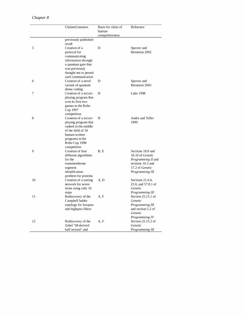
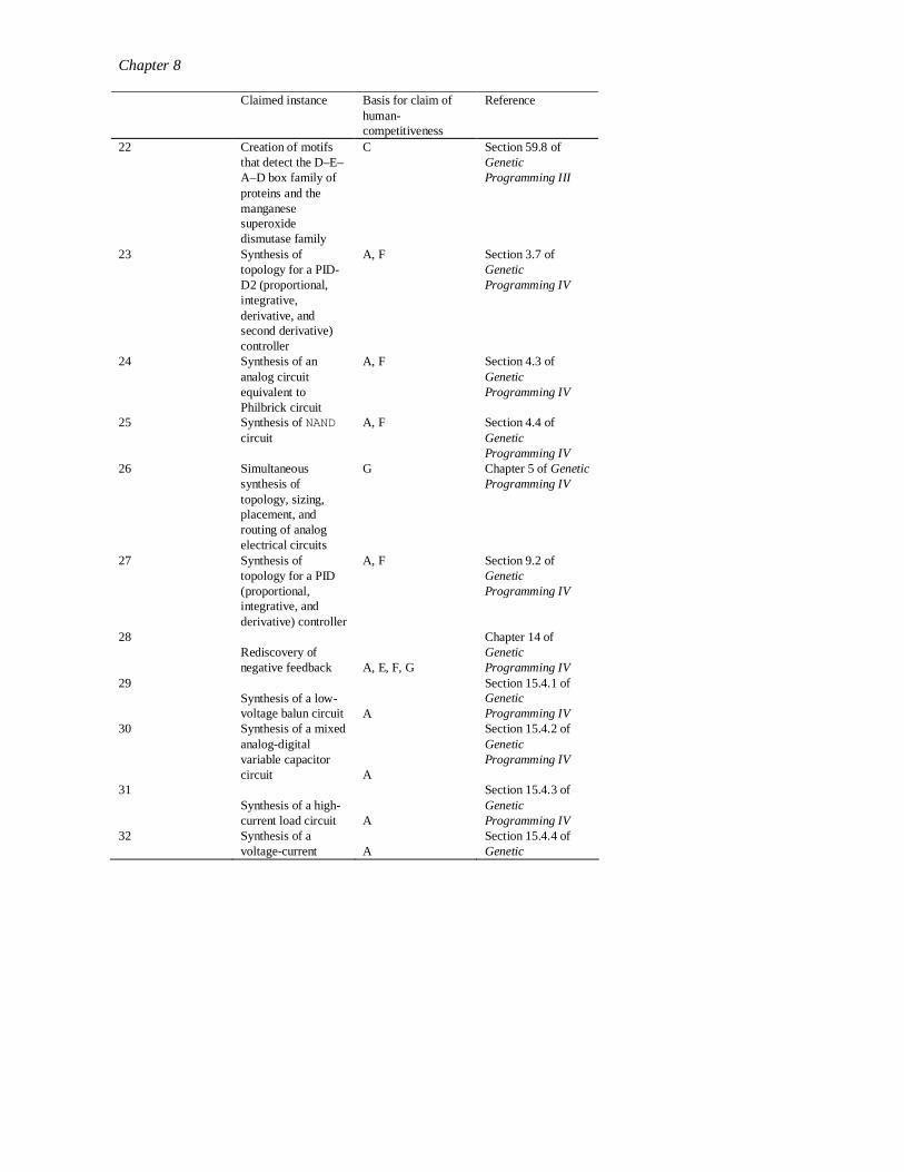
Table 2 lists the 36 human-competitive instances (of which we are aware) where genetic programming has produced human-competitive results. Each entry in the table is accompanied by the criteria (from table 1) that establish the basis for the claim of human-competitiveness.

Table 2. [Enter a caption for this table] Claimed instance Basis for claim of

human-competitiveness

Reference

1 Creation of a better-than-classical quantum algorithm for the Deutsch-Jozsa “early promise” problem

B, F Spector, Barnum, and Bernstein 1998

2 Creation of a better-than-classical quantum algorithm for Grover’s database search problem

B, F Spector, Barnum, and Bernstein 1999

3 Creation of a quantum algorithm for the depth-two AND/OR query problem that is better than any previously published result

D Spector, Barnum, Bernstein, and Swamy 1999; Barnum, Bernstein, and Spector 2000

4 Creation of a quantum algorithm for the depth-one OR query problem that is better than any

D Barnum, Bernstein, and Spector 2000

Chapter 8

Claimed instance Basis for claim of human-competitiveness

Reference

previously published result

5 Creation of a protocol for communicating information through a quantum gate that was previously thought not to permit such communication

D Spector and Bernstein 2002

6 Creation of a novel variant of quantum dense coding

D Spector and Bernstein 2002

7 Creation of a soccer-playing program that won its first two games in the Robo Cup 1997 competition

H Luke 1998

8 Creation of a soccer-playing program that ranked in the middle of the field of 34 human-written programs in the Robo Cup 1998 competition

H Andre and Teller 1999

9 Creation of four different algorithms for the transmembrane segment identif ication problem for proteins

B, E Sections 18.8 and 18.10 of Genetic Programming II and sections 16.5 and 17.2 of Genetic Programming III

10 Creation of a sorting network for seven items using only 16 steps

A, D Sections 21.4.4, 23.6, and 57.8.1 of Genetic Programming III

11 Rediscovery of the Campbell ladder topology for lowpass and highpass filters

A, F Section 25.15.1 of Genetic Programming III and section 5.2 of Genetic Programming IV

12 Rediscovery of the Zobel “M-derived half section” and

A, F Section 25.15.2 of Genetic Programming III

Chapter 8


Reference

“constant K” f ilter sections

13 Rediscovery of the Cauer (elliptic) topology for filters

A, F Section 27.3.7 of Genetic Programming III

14 Automatic decomposition of the problem of synthesizing a crossover filter

A, F Section 32.3 of Genetic Programming III

15 Rediscovery of a recognizable voltage gain stage and a Darlington emitter-follower section of an amplifier and other circuits


16 Synthesis of 60 and 96 decibel amplif iers


17 Synthesis of analog computational circuits for squaring, cubing, square root, cube root, logarithm, and Gaussian functions

A, D, G Section 47.5.3 of Genetic Programming III

18 Synthesis of a real-time analog circuit for time-optimal control of a robot

G Section 48.3 of Genetic Programming III

19 Synthesis of an electronic thermometer

A, G Section 49.3 of Genetic Programming III

20 Synthesis of a voltage reference circuit

A, G Section 50.3 of Genetic Programming III

21 Creation of a cellular automata rule for the majority classif ication problem that is better than the Gacs-Kurdyumov-Levin (GKL) rule and all other known rules written by humans

D, E and section 58.4 of Genetic Programming III

Chapter 8


Reference

22 Creation of motifs that detect the D–E–A–D box family of proteins and the manganese superoxide dismutase family

C Section 59.8 of Genetic Programming III

23 Synthesis of topology for a PID-D2 (proportional, integrative, derivative, and second derivative) controller

A, F Section 3.7 of Genetic Programming IV

24 Synthesis of an analog circuit equivalent to Philbrick circuit


25 Synthesis of NAND circuit


26 Simultaneous synthesis of topology, sizing, placement, and routing of analog electrical circuits

G Chapter 5 of Genetic Programming IV

27 Synthesis of topology for a PID (proportional, integrative, and derivative) controller


28 Rediscovery of negative feedback A, E, F, G

Chapter 14 of Genetic Programming IV

29 Synthesis of a low-voltage balun circuit A

Section 15.4.1 of Genetic Programming IV

30 Synthesis of a mixed analog-digital variable capacitor circuit A


31 Synthesis of a high-current load circuit A


32 Synthesis of a voltage-current A

Section 15.4.4 of Genetic

Chapter 8


Reference

conversion circuit Programming IV 33

Synthesis of a cubic signal generator A


34 Synthesis of a tunable integrated active f ilter A


35 Creation of PID tuning rules that outperform the Ziegler-Nichols and Astrom-Hagglund tuning rules

A, B, D, E, F, G Chapter 12 of Genetic Programming IV

36 Creation of three non-PID controllers that outperform a PID controller that uses the Ziegler-Nichols or Astrom-Hagglund tuning rules

A, B, D, E, F, G Chapter 13 of Genetic Programming IV

There are now 23 instances where genetic programming has duplicated the functionality of a previously patented invention, infringed a previously patented invention, or created a patentable new invention (see criterion A in Table 1). Speci fically, there are 15 instances where genetic programming has created an entity that either infringes or duplicates the functionality of a previously patented 20th-century invention, six instances where genetic programming has done the same with respect to an invention patented after January 1, 2000, and two instances where genetic programming has created a patentable new invention. The two new inventions are general-purpose controllers that outperform controllers employing tuning rules that have been in widespread use in industry for most of the 20th century.

7. PROMISING APPLICATION AREAS FOR GENETIC PROGRAMMING AND OTHER METHODS OF GENETIC AND EVOLUTIONARY COMPUTATION

Since its early beginnings, the field of genetic and evolutionary computation has produced a cornucopia of results.

Chapter 8

Genetic programming and other methods of genetic and evolutionary computation may be especially productive in areas having some or all of the following characteristics: – where the interrelationships among the relevant variables are unknown or

poorly understood (or where it is suspected that the current understanding may possibly be wrong),

– where finding the size and shape of the ultimate solution to the problem is a major part of the problem,

– where large amounts of primary data requiring examination, classification, and integration is accumulating in computer readable form,

– where there are good simulators to test the performance of tentative solutions to a problem, but poor methods to directly obtain good solutions,

– where conventional mathematical analysis does not, or cannot, provide analytic solutions,

– where an approximate solution is acceptable (or is the only result that is ever likely to be obtained), or

– where small improvements in performance are routinely measured (or easily measurable) and highly prized.

8. GENETIC PROGRAMMING THEORY

Genetic programming is a search technique that explores the space of computer programs. As discussed above, the search for solutions to a problem starts from a group of points (random programs) in this search space. Those points that are of above average quality are then used to generate a new generation of points through crossover, mutation, reproduction and possibly other genetic operations. This process is repeated over and over again until a termination criterion is satisfied.

If we could visualize this search, we would often find that initially the population looks a bit like a cloud of randomly scattered points, but that, generation after generation, this cloud changes shape and moves in the search space following a well defined trajectory. Because genetic programming is a stochastic search technique, in different runs we would observe different trajectories. These, however, would very likely show very clear regularities to our eye that could provide us with a deep understanding of how the algorithm is searching the program space for the solutions to a given problem. We could probably readil y see, for example, why genetic programming is successful in finding solutions in certain runs and with certain parameter settings, and unsuccessful in/with others.

Chapter 8

Unfortunately, it is normally impossible to exactly visualize the program search space due to its high dimensionality and complexity, and so we cannot just use our senses to understand and predict the behavior of genetic programming.

In this situation, one approach to gain an understanding of the behavior of a genetic programming system is to perform many real runs and record the variations of certain numerical descriptors (like the average fitness or the average size of the programs in the population at each generation, the average difference between parent and offspring fitness, etc.). Then, one can try to hypothesize explanations about the behavior of the system that are compatible with (and could explain) the empirical observations.

This exercise is very error prone, though, because a genetic programming system is a complex adaptive system with zil lions of degrees of freedom. So, any small number of statistical descriptors is l ikely to be able to capture only a tiny fraction of the complexities of such a system. This is why in order to understand and predict the behavior of genetic programming (and indeed of most other evolutionary algorithms) in precise terms we need to define and then study mathematical models of evolutionary search.

Schema theories are among the oldest, and probably the best-known classes of models of evolutionary algorithms. A schema (pl. schemata) is a set of points in the search space sharing some syntactic feature. Schema theories provide information about the properties of individuals of the population belonging to any schema at a given generation in terms of quantities measured at the previous generation, without having to actuall y run the algorithm.

For example, in the context of genetic algorithms operating on binary strings, a schema is, syntactically, a string of symbols from the alphabet { 0,1,*} , like *10*1. The character * is interpreted as a “don't care'' symbol, so that, semanticall y, a schema represents a set of bit strings. For example the schema *10*1 represents a set of four strings: { 01001, 01011, 11001, 11011} .

Typically schema theorems are descriptions of how the number (or the proportion) of members of the population belonging to (or matching) a schema varies over time.

For a given schema H the selection/crossover/mutation process can be seen as a Bernoulli trial, because a newly created individual either samples or does not sample H. Therefore, the number of individuals sampling H at the next generation, m(H,t+1) is a binomial stochastic variable. So, if we denote with α(Η,t) the success probability of each trial (i.e. the probability that a newly created individual samples H), an exact schema theorem is simply

Chapter 8

E[m(H,t+1)]=M α(H,t)

where M is the population size and E[.] is the expectation operator. Holland's and other approximate schema theories (Holland 1975; Goldberg 1989; Whitley 1994) normally provide a lower bound for α(H,t) or, equivalently, for E[m(H,t+1)]. For example, several schema theorems for one-point crossover and point mutation have the following form

�� ×

−×−−≥ σα

1

)(1)1)(,(),( )(

N

HLpptHptH c

HOm

where m(H,t) is number of individuals in the schema H at generation t, M is the population size, p(H,t) is the selection probability for strings in H at generation t, pm is the mutation probability, O(H) is the schema order, i.e. number of defining bits, pc is the crossover probability, L(H) is the defining length, i.e. distance between the furthest defining bits in H, and N is the bitstring length. The factor σ differs in the different formulation of the schema theorem: σ=1-m(H,t)/M in (Holland, 1975) (where one of the parents was chosen randomly, irrespective of fitness), σ=1 in (Goldberg, 1989) and σ=1-p(H,t) in (Whitley, 1994).

More recently, Stephens and collaborators (Stephens and Waelbroeck 1997; Stephens and Waelbroeck 1999) have produced exact formulations for α(H,t), which are now known as “ exact'' schema theorems for genetic algorithms. These, however, are beyond the scope of this chapter.

The theory of schemata in genetic programming has had a slow start, one of the difficulties being that the variable size tree structure in genetic programming makes it more difficult to develop a definition of genetic programming schema having the necessary power and flexibility. Several alternatives have been proposed in the literature, which define schemata as composed of one or multiple trees or fragments of trees. Here, however, we will focus only on a particular one, which was proposed in (Poli and Langdon, 1997; Poli and Langdon 1998) since this has later been used to develop an exact and general schema theory for genetic programming (Poli 2001; Langdon and Poli 2002).

In this definition, syntactically, a genetic programming schema is a tree with some “don’ t care” nodes which represents exactly one primitive function or terminal. Semantically, a schema represents all programs that match its size, shape and defining (non-“don’ t care'”) nodes. For example, the schema

H = ( DON' T- CARE x ( + y DON' T- CARE) ) represents the programs (+ x (+ y x)), (+ x (+ y y)), (*

x (+ y x)), etc.

Chapter 8

The exact schema theorem in (Poli 2001) gives the expected proportion of individuals matching a schema in the next generation as a function of information about schemata in the current generation. The calculation is non-trivial, but it is easier than one might think.

Let us assume, for simplicity, that only reproduction and (one-offspring) crossover are performed. Because these two operators are mutually exclusive, for a generic schema H we then have:

[ ]]crossoverbyproducedisHmatchingoffspringAnPr[

onreproductiviaobtainedisHinindividualAnPr),(

+=tHα

Then, assuming that reproduction is performed with probability pr and crossover with probability pc (with pr+pc=1), we obtain

[ ]��

��×+

×=

Hp

HptH

c

r

matchesoffspringthethatsuchare

pointscrossovertheandparentsThePr

cloningforselectedisinindividualAnPr),(α

Clearly, the first probability in this expression is simply the selection probability for members of the schema H as dictated by, say, fitness-proportionate selection or tournament selection. So,

[ ] ),(cloningforinindividualanSelectingPr tHpH =

We now need to calculate the second term in α(Η,t), that is the probability that the parents have shapes and contents compatible with the creation of an offspring matching H, and that the crossover points in the two parents are such that exactly the necessary material to create such an offspring is swapped. This is the harder part of the calculation.

An observation that helps simplify the problem is that, although the probability of choosing a particular crossover point in a parent depends on the actual size and shape of such a parent, the process of crossover point selection is independent from the actual primitives present in the parent tree. So, for example, the probability of choosing any crossover point in the program (+ x (+ y x)) is identical to the probability of choosing any crossover point in the program (AND D1 (OR D1 D2)). This is because the two programs have exactly the same shape. Thanks to this observation we can write

Chapter 8

��×

��=

��

� �

Hji

lk

lkji

H

lklk

ji

in offspring an produce and pointsat over crossed

if that such , and shapes withparents SelectingPr

andshapesinand

pointscrossover ChoosingPr

matchesoffspringthethatsuchare

pointscrossovertheandparentsThePr

,shapesparentofpairsallFor

andshapesin,points

crossoverallFor

If, for simplicity, we assume that crossover points are selected with uniform probability, then

lklkji shapeinNodes1

shapeinNodes1

andshapesinand

pointscrossover ChoosingPr ×=��

So, we are left with the problem of calculating the probability of selecting (for crossover) parents having specific shapes while at the same time having an arrangement of primitives such that, if crossed over at certain predefined points, they produce an offspring matching a particular schema of interest.

Again, here we can simplify the problem by considering how crossover produces offspring: it excises a subtree rooted at the chosen crossover point in a parent, and replaces it with a subtree excised from the chosen crossover point in the other parent. This means that the offspring will have the right shape and primitives to match the schema of interest if and only if, after the excision of the chosen subtree, the first parent has shape and primitives compatible with the schema, and the subtree to be inserted has shape and primitives compatible with the schema. That is:

��×

��=

��

iHj

l

iHi

k

Hji

lk

w.r.t. ofpart lower thematches point crossover .part w.r.t

lower its that such shape hparent wit donating-subtreea SelectingPr

w.r.t. ofpart upper thematches point crossover .part w.r.t

upper its that such shape hparent wit donating-roota SelectingPr

in offspring an produce and pointsat over crossed

if that such , and shapes withparents SelectingPr

These two selection probabilities can be calculated exactly. However, the calculation requires the introduction of several other concepts and notation,

Chapter 8

which are beyond the introductory nature of this chapter. These definitions, the complete theory and a number of examples and applications can be found in (Poli 2001; Langdon and Poli 2002; Poli and McPhee 2003a; Poli and McPhee 2003b).

Although exact schema theoretic models of genetic programming have become available only very recently, they have already started shedding some light on fundamental questions regarding the how and why genetic programming works. Importantly, other important theoretical models of genetic programming have recently been developed which add even more to our theoretical understanding of genetic programming. These, however, go well beyond the scope of this chapter. The interested reader should consult Foundations of Genetic Programming (Langdon and Poli, 2002) and (Poli and McPhee 2003a; Poli and McPhee 2003b) for more information.

9. CONCLUSIONS

In his seminal 1948 paper entitled “Intelligent Machinery,” Turing identified three ways by which human-competitive machine intelligence might be achieved. In connection with one of those ways, Turing (1948) said:

“There is the genetical or evolutionary search by which a combination of genes is looked for, the criterion being the survival value.”

Turing did not specify how to conduct the “genetical or evolutionary search” for machine intelligence. In particular, he did not mention the idea of a population-based parallel search in conjunction with sexual recombination (crossover) as described in John Holland’s 1975 book Adaptation in Natural and Artificial Systems. However, in his 1950 paper “Computing Machinery and Intelligence,” Turing (1950) did point out

“We cannot expect to find a good child-machine at the first attempt. One must experiment with teaching one such machine and see how well it learns. One can then try another and see if it is better or worse. There is an obvious connection between this process and evolution, by the identifications

“Structure of the child machine = Hereditary material

“Changes of the child machine = Mutations

Chapter 8

"Natural selection = Judgment of the experimenter”

That is, Turing perceived in 1948 and 1950 that one possibly productive approach to machine intelligence would involve an evolutionary process in which a description of a computer program (the hereditary material) undergoes progressive modification (mutation) under the guidance of natural selection (i.e., selective pressure in the form of what we now call “fitness”).

Today, many decades later, we can see that indeed Turing was right. Genetic programming has started fulfilling Turing’s dream by providing us with a systematic method, based on Darwinian evolution, for getting computers to automatically solve hard real-life problems. To do so, it simply requires a high-level statement of what needs to be done (and enough computing power).

Turing also understood the need to evaluate objectively the behaviour exhibited by machines, to avoid human biases when assessing their intelligence. This led him to propose an imitation game, now know as the Turing test for machine intelligence, whose goals are wonderfully summarised by Arthur Samuel’s position statement quoted in the introduction of this chapter.

At present genetic programming is certainly not in a position to produce computer programs that would pass the full Turing test for machine intelligence, and it might not be ready for this immense task for centuries. Nonetheless, thanks to the constant technological improvements in genetic programming technology, in its theoretical foundations and in computing power, genetic programming has been able to solve tens of difficult problems with human-competitive results (see Table 2) in the recent past. These are a small step towards fulfilling Turing and Samuel’s dreams, but they are also early signs of things to come. It is, indeed, arguable that in a few years’ time genetic programming will be able to routinely and competently solve important problems for us in a variety of specific domains of application, even when running on a single personal computer, thereby becoming an essential collaborator for many of human activities. This, we believe, will be a remarkable step forward towards achieving true, human-competitive machine intelligence.

SOURCES OF ADDITIONAL INFORMATION ABOUT GENETIC PROGRAMMING

Sources of information about genetic programming include − Genetic Programming: On the Programming of Computers by Means of Natural

Selection (Koza 1992a) and the accompanying videotape Genetic Programming: The Movie (Koza and Rice 1992);

Chapter 8

− Genetic Programming II: Automatic Discovery of Reusable Programs (Koza 1994a) and the accompanying videotape Genetic Programming II Videotape: The Next Generation (Koza 1994b);

− Genetic Programming III: Darwinian Invention and Problem Solving (Koza, Bennett, Andre, and Keane 1999) and the accompanying videotape Genetic Programming III Videotape: Human-Competitive Machine Intelligence (Koza, Bennett, Andre, Keane, and Brave 1999);

− Genetic Programming IV. Routine Human-Competitive Machine Intelligence (Koza, Keane, Streeter, Mydlowec, Yu, and Lanza 2003);

− Genetic ProgrammingAn Introduction (Banzhaf, Nordin, Keller, and Francone 1998); − Genetic Programming and Data Structures: Genetic Programming + Data Structures =

Automatic Programming! (Langdon 1998) in the series on genetic programming from Kluwer Academic Publishers;

− Automatic Re-engineering of Software Using Genetic Programming (Ryan 1999) in the series on genetic programming from Kluwer Academic Publishers;

− Data Mining Using Grammar Based Genetic Programming and Applications (Wong and Leung 2000) in the series on genetic programming from Kluwer Academic Publishers;

− Principia Evolvica: Simulierte Evolution mit Mathematica (Jacob 1997, in German) and Illustrating Evolutionary Computation with Mathematica (Jacob 2001);

− Genetic Programming (Iba 1996, in Japanese); − Evolutionary Program Induction of Binary Machine Code and Its Application (Nordin

1997); − Foundations of Genetic Programming (Langdon and Poli 2002); − Emergence, Evolution, Intelligence: Hydroinformatics (Babovic 1996); − Theory of Evolutionary Algorithms and Application to System Synthesis (Blickle 1997); − edited collections of papers such as the three Advances in Genetic Programming books

from the MIT Press (Kinnear 1994; Angeline and Kinnear 1996; Spector, Langdon, O’Reilly, and Angeline 1999);

− the proceedings of the Genetic Programming Conference held between 1996 and 1998 (Koza, Goldberg, Fogel, and Riolo 1996; Koza, Deb, Dorigo, Fogel, Garzon, Iba, and Riolo 1997; Koza, Banzhaf, Chellapilla, Deb, Dorigo, Fogel, Garzon, Goldberg, Iba, and Riolo 1998);

− the proceedings of the annual Genetic and Evolutionary Computation Conference (GECCO) (combining the formerly annual Genetic Programming Conference and the formerly biannual International Conference on Genetic Algorithms) operated by the International Society for Genetic and Evolutionary Computation (ISGEC) and held starting in 1999 (Banzhaf, Daida, Eiben, Garzon, Honavar, Jakiela, and Smith 1999; Whitley, Goldberg, Cantu-Paz, Spector, Parmee, and Beyer 2000; Spector, Goodman, Wu, Langdon, Voigt, Gen, Sen, Dorigo, Pezeshk, Garzon, and Burke 2001; Langdon, Cantu-Paz, Mathias, Roy, Davis, Poli, Balakrishnan, Honavar, Rudolph, Wegener, Bull, Potter, Schultz, Miller, Burke, and Jonoska 2002);

− the proceedings of the annual Euro-GP conferences held starting in 1998 (Banzhaf, Poli, Schoenauer, and Fogarty 1998; Poli, Nordin, Langdon, and Fogarty 1999; Poli, Banzhaf, Langdon, Miller, Nordin, and Fogarty 2000; Miller, Tomassini, Lanzi, Ryan, Tettamanzi, and Langdon 2001; Foster, Lutton, Miller, Ryan, and Tettamanzi 2002);

− the proceedings of the Workshop of Genetic Programming Theory and Practice organized by the Center for Study of Complex Systems of the University of Michigan (to be published in 2003 by Kluwer Academic Publishers),

− the Genetic Programming and Evolvable Machines journal (from Kluwer Academic Publishers) started in April 2000;

Chapter 8

− web sites such as www.genetic-programming.org and www.genetic-programming.com;

− LISP code for implementing genetic programming, available in Genetic Programming (Koza 1992a), and genetic programming implementations in other languages such as C or Java (Web sites such as www.genetic-programming.org contain links to computer code in various programming languages);

− early papers on genetic programming, such as the Stanford University Computer Science Department technical report Genetic Programming: A Paradigm for Genetically Breeding Populations of Computer Programs to Solve Problems (Koza 1990a) and the paper “Hierarchical Genetic Algorithms Operating on Populations of Computer Programs,” presented at the 11th International Joint Conference on Artificial Intelligence in Detroit (Koza 1989);

− an annotated bibliography of the first 100 papers on genetic programming (other than those of which John Koza was the author or co-author) in appendix F of Genetic Programming II: Automatic Discovery of Reusable Programs (Koza 1994a); and

− William Langdon’s bibliography on genetic programming at http://www.cs.bham.ac.uk/~wbl/biblio/ or http://liinwww.ira.uka.de/bibliography/Ai/genetic.programming.html. This bibliography is the most extensive in the field and contains over 3,034 papers (as of January 2003) and over 880 authors. It provides on-line access to many of the papers.

BIBLIOGRAPHY

Andre, David and Teller, Astro. 1999. Evolving team Darwin United. In Asada, Minoru and Kitano, Hiroaki (editors). RoboCup-98: Robot Soccer World Cup II. Lecture Notes in Computer Science. Volume 1604. Berlin: Springer-Verlag. Pages 346–352.

Angeline, Peter J. and Kinnear, Kenneth E. Jr. (editors). 1996. Advances in Genetic Programming 2. Cambridge, MA: The MIT Press.

Babovic, Vladan. 1996. Emergence, Evolution, Intell igence: Hydroinformatics. Rotterdam, The Netherlands: Balkema Publishers.

Banzhaf, Wolfgang, Daida, Jason, Eiben, A. E., Garzon, Max H., Honavar, Vasant, Jakiela, Mark, and Smith, Robert E. (editors). 1999. GECCO-99: Proceedings of the Genetic and Evolutionary Computation Conference, July 13–17, 1999, Orlando, Florida USA. San Francisco, CA: Morgan Kaufmann.

Banzhaf, Wolfgang, Nordin, Peter, Keller, Robert E., and Francone, Frank D. 1998. Genetic Programming: An Introduction. San Francisco, CA: Morgan Kaufmann and Heidelberg: dpunkt.

Banzhaf, Wolfgang, Poli, Riccardo, Schoenauer, Marc, and Fogarty, Terence C. 1998. Genetic Programming: First European Workshop. EuroGP’98. Paris, France, April 1998 Proceedings. Lecture Notes in Computer Science. Volume 1391. Berlin, Germany: Springer-Verlag.

Barnum, H., Bernstein, H.J. and Spector, Lee. 2000. Quantum circuits for OR and AND of ORs. Journal of Physics A: Mathematical and General. 33(45)8047–8057. November 17, 2000.

Blickle, Tobias. 1997. Theory of Evolutionary Algorithms and Application to System Synthesis. TIK-Schriftenreihe Nr. 17. Zurich, Switzerland: vdf Hochschul Verlag AG an der ETH Zuerich.

Chapter 8

Foster, James A., Lutton, Evelyne, Miller, Julian, Ryan, Conor, and Tettamanzi, Andrea G. B. (editors). 2002. Genetic Programming: 5th European Conference, EuroGP 2002, Kinsale, Ireland, April 2002 Proceedings.

Goldberg, David E. 1989. Genetic Algorithms in Search, Optimization, and Machine Learning. Reading, MA: Addison-Wesley.

Holland, John H. 1975. Adaptation in Natural and Artificial Systems: An Introductory Analysis with Applications to Biology, Control, and Artificial Intell igence. Ann Arbor, MI: University of Michigan Press. Second edition. Cambridge, MA: The MIT Press 1992.

Iba, Hitoshi. 1996. Genetic Programming. Tokyo: Tokyo Denki University Press. In Japanese.

Jacob, Christian. 1997. Principia Evolvica: Simulierte Evolution mit Mathematica. Heidelberg, Germany: dpunkt.verlag.

Jacob, Christian. 2001. Illustrating Evolutionary Computation with Mathematica. San Francisco: Morgan Kaufmann.

Kinnear, Kenneth E. Jr. (editor). 1994. Advances in Genetic Programming. Cambridge, MA: MIT Press.

Koza, John R. 1989. Hierarchical genetic algorithms operating on populations of computer programs. In Proceedings of the 11th International Joint Conference on Arti ficial Intell igence. San Mateo, CA: Morgan Kaufmann. Volume I. Pages 768–774.

Koza, John R. 1990a. Genetic Programming: A Paradigm for Genetically Breeding Populations of Computer Programs to Solve Problems. Stanford University Computer Science Department technical report STAN-CS-90-1314. June 1990.

Koza, John R. 1992a. Genetic Programming: On the Programming of Computers by Means of Natural Selection. Cambridge, MA: MIT Press.

Koza, John R. 1994a. Genetic Programming II: Automatic Discovery of Reusable Programs. Cambridge, MA: MIT Press.

Koza, John R. 1994b. Genetic Programming II Videotape: The Next Generation. Cambridge, MA: MIT Press.

Koza, John R. 1994c. Architecture-Altering Operations for Evolving the Architecture of a Multi-Part Program in Genetic Programming. Stanford University Computer Science Department technical report STAN-CS-TR-94-1528. October 21, 1994.

Koza, John R. 1995. Gene duplication to enable genetic programming to concurrently evolve both the architecture and work-performing steps of a computer program. Proceedings of the 14th International Joint Conference on Artificial Intelligence. San Francisco: Morgan Kaufmann. Pages 734–740.

Koza, John R., Banzhaf, Wolfgang, Chellapilla, Kumar, Deb, Kalyanmoy, Dorigo, Marco, Fogel, David B., Garzon, Max H., Goldberg, David E., Iba, Hitoshi, and Riolo, Rick. (editors). 1998. Genetic Programming 1998: Proceedings of the Third Annual Conference. San Francisco, CA: Morgan Kaufmann.

Koza, John R., Bennett III, Forrest H, Andre, David, and Keane, Martin A. 1999. Genetic Programming III: Darwinian Invention and Problem Solving. San Francisco, CA: Morgan Kaufmann.

Koza, John R., Bennett III, Forrest H, Andre, David, Keane, Martin A., and Brave, Scott. 1999. Genetic Programming III Videotape: Human-Competitive Machine Intell igence. San Francisco, CA: Morgan Kaufmann.

Koza, John R., Deb, Kalyanmoy, Dorigo, Marco, Fogel, David B., Garzon, Max, Iba, Hitoshi, and Riolo, Rick L. (editors). Genetic Programming 1997: Proceedings of the Second Annual Conference, July 13–16, 1997, Stanford University. San Francisco, CA: Morgan Kaufmann.

Chapter 8

Koza, John R., Goldberg, David E., Fogel, David B., and Riolo, Rick L. (editors). 1996. Genetic Programming 1996: Proceedings of the First Annual Conference, July 28–31, 1996, Stanford University. Cambridge, MA: MIT Press.

Koza, John R., Keane, Martin A., Streeter, Matthew J., Mydlowec, William, Yu, Jessen, and Lanza, Guido. 2003. Genetic Programming IV: Routine Human-Competitive Machine Intell igence. Kluwer Academic Publishers.

Koza, John R., and Rice, James P. 1992. Genetic Programming: The Movie. Cambridge, MA: The MIT Press.

Langdon, William B. 1998. Genetic Programming and Data Structures: Genetic Programming + Data Structures = Automatic Programming! Amsterdam: Kluwer.

Langdon, W. B., Cantu-Paz, E., Mathias, K., Roy, R., Davis, D., Poli, R., Balakrishnan, K., Honavar, V., Rudolph, G., Wegener, J., Bull, L., Potter, M. A., Schultz, A. C., Miller, J. F., Burke, E., and Jonoska, N. (editors). 2002. Proceedings of the 2002 Genetic and Evolutionary Computation Conference. San Francisco, CA: Morgan Kaufmann.

Langdon, William B. and Poli, Riccardo. 2002. Foundations of Genetic Programming. Springer-Verlag.

Luke, Sean. 1998. Genetic programming produced competitive soccer softbot teams for RoboCup97. In Koza, John R., Banzhaf, Wolfgang, Chellapilla, Kumar, Deb, Kalyanmoy, Dorigo, Marco, Fogel, David B., Garzon, Max H., Goldberg, David E., Iba, Hitoshi, and Riolo, Rick. (editors). Genetic Programming 1998: Proceedings of the Third Annual Conference, July 22–25, 1998, University of Wisconsin, Madison, Wisconsin. San Francisco, CA: Morgan Kaufmann. Pages 214–222.

Miller, Julian, Tomassini, Marco, Lanzi, Pier Luca, Ryan, Conor, Tettamanzi, Andrea G. B., and Langdon, William B. (editors). 2001. Genetic Programming: 4th European Conference, EuroGP 2001, Lake Como, Italy, April 2001 Proceedings. Berlin: Springer.

Nordin, Peter. 1997. Evolutionary Program Induction of Binary Machine Code and Its Application. Munster, Germany: Krehl Verlag.

Poli, R. and Langdon, W.B. 1997. A new schema theory for genetic programming with one-point crossover and point mutation. In Koza, J. R., Deb, K., Dorigo, M., Fogel, D. B., Garzon, M., Iba, H., and Riolo, R. L., editors, Genetic Programming 1997: Proceedings of the Second Annual Conference, pages 278-285, Stanford University, CA, USA. Morgan Kaufmann.

Poli, R. and Langdon, W.B. 1998. Schema theory for genetic programming with one-point crossover and point mutation. Evolutionary Computation, 6(3):231-252.

Poli, R. and McPhee, N. F. 2001. Exact schema theorems for GP with one-point and standard crossover operating on linear structures and their application to the study of the evolution of size. In Miller, J. F., Tomassini, M., Lanzi, P. L., Ryan, C., Tettamanzi, A. G. B., and Langdon, W. B., editors, Genetic Programming, Proceedings of EuroGP'2001, volume 2038 of LNCS, pages 126-142, Lake Como, Italy. Springer-Verlag.

Poli, R. and McPhee, N. F. 2003a.General schema theory for genetic programming with subtree-swapping crossover: Part I. Evolutionary Computation, 11(1):53-66.

Poli, R. and McPhee, N. F. 2003b.General schema theory for genetic programming with subtree-swapping crossover: Part II. Evolutionary Computation, 11(2)..

Poli, Riccardo, Nordin, Peter, Langdon, William B., and Fogarty, Terence C. 1999. Genetic Programming: Second European Workshop, EuroGP’99. Proceedings. Lecture Notes in Computer Science. Volume 1598. Berlin, Germany: Springer-Verlag.

Poli, Riccardo, Banzhaf, Wolfgang, Langdon, William B., Miller, Julian, Nordin, Peter, and Fogarty, Terence C. 2000. Genetic Programming: European Conference, EuroGP 2000, Edinburgh, Scotland, UK, April 2000, Proceedings. Lecture Notes in Computer Science. Volume 1802. Berlin, Germany: Springer-Verlag.

Chapter 8

Ryan, Conor. 1999. Automatic Re-engineering of Software Using Genetic Programming. Amsterdam: Kluwer Academic Publishers.

Samuel, Arthur L. 1983. AI: Where it has been and where it is going. Proceedings of the Eighth International Joint Conference on Artificial Intel ligence. Los Altos, CA: Morgan Kaufmann. Pages 1152–1157.

Spector, Lee, Barnum, Howard, and Bernstein, Herbert J. 1998. Genetic programming for quantum computers. In Koza, John R., Banzhaf, Wolfgang, Chellapilla, Kumar, Deb, Kalyanmoy, Dorigo, Marco, Fogel, David B., Garzon, Max H., Goldberg, David E., Iba, Hitoshi, and Riolo, Rick. (editors). Genetic Programming 1998: Proceedings of the Third Annual Conference. San Francisco, CA: Morgan Kaufmann. Pages 365–373.

Spector, Lee, Barnum, Howard, and Bernstein, Herbert J. 1999. Quantum computing applications of genetic programming. In Spector, Lee, Langdon, William B., O’Reilly, Una-May, and Angeline, Peter (editors). Advances in Genetic Programming 3. Cambridge, MA: The MIT Press. Pages 135–160.

Spector, Lee, Barnum, Howard, Bernstein, Herbert J., and Swamy, N. 1999. Finding a better-than-classical quantum AND/OR algorithm using genetic programming. In IEEE. Proceedings of 1999 Congress on Evolutionary Computation. Piscataway, NJ: IEEE Press. Pages 2239–2246.

Spector, Lee, and Bernstein, Herbert J. 2002. Communication capacities of some quantum gates, discovered in part through genetic programming. In Proceedings of the Sixth International Conference on Quantum Communication, Measurement, and Computing. Paramus, NJ: Rinton Press.

Spector, Lee, Goodman, E., Wu, A., Langdon, William B., Voigt, H. -M., Gen, M., Sen, S., Dorigo, Marco, Pezeshk, S., Garzon, Max, and Burke, E. (editors). 2001. Proceedings of the Genetic and Evolutionary Computation Conference, GECCO-2001. San Francisco, CA: Morgan Kaufmann.

Spector, Lee, Langdon, William B., O’Reilly, Una-May, and Angeline, Peter (editors). 1999. Advances in Genetic Programming 3. Cambridge, MA: The MIT Press.

Stephens, C. R. and Waelbroeck, H. 1997. Effective degrees of freedom in genetic algorithms and the block hypothesis. In Back, Thomas (editor). 1997. Genetic Algorithms: Proceedings of the Seventh International Conference. San Francisco, CA: Morgan Kaufmann. Pages 34–40.

Stephens, C. R. and Waelbroeck, H. 1999. Schemata evolution and building blocks. Evolutionary Computation, 7(2):109-124.

Turing, Alan M. 1948. Intelligent machinery. Reprinted in Ince, D. C. (editor). 1992. Mechanical Intelligence: Collected Works of A. M. Turing. Amsterdam: North Holland. Pages 107–127. Also reprinted in Meltzer, B. and Michie, D. (editors). 1969. Machine Intell igence 5. Edinburgh: Edinburgh University Press.

Turing, Alan M. 1950. Computing machinery and intelligence. Mind. 59(236)433–460. Reprinted in Ince, D. C. (editor). 1992. Mechanical Intelligence: Collected Works of A. M. Turing. Amsterdam: North Holland. Pages 133–160.

Whitley, L. D. 1994. A Genetic Algorithm Tutorial. Statistics and Computing, 4:65-85. Whitley, Darrell, Goldberg, David, Cantu-Paz, Erick, Spector, Lee, Parmee, Ian, and Beyer,

Hans-Georg (editors). 2000. GECCO-2000: Proceedings of the Genetic and Evolutionary Computation Conference, July 10–12, 2000, Las Vegas, Nevada. San Francisco: Morgan Kaufmann.

Wong, Man Leung and Leung, Kwong Sak. 2000. Data Mining Using Grammar Based Genetic Programming and Applications. Amsterdam: Kluwer Academic Publishers.

Chapter 8 A Genetic Programming Tutorial - PBworksphil415.pbworks.com/f/JKTutorial.pdf · Chapter 8 Chapter 8 A Genetic Programming Tutorial John 1R. Koza and Riccardo Poli2 1 St

Documents