Chapter 7: The Cost of Production 1 of 50 Copyright © 2009 Pearson Education, Inc. Publishing as Prentice Hall • Microeconomics • Pindyck/Rubinfeld, 8e. CHAPTER 7 OUTLINE 7.1 Measuring Cost: Which Costs Matter? 7.2 Cost in the Short Run 7.3 Cost in the Long Run 7.4 Long-Run versus Short-Run Cost Curves 7.5 Production with Two Outputs— Economies of Scope 7.6 Dynamic Changes in Costs—The Learning Curve 7.7 Estimating and Predicting Cost

Chapter 7: The Cost of Production 1 of 50 Copyright © 2009 Pearson Education, Inc. Publishing as Prentice Hall Microeconomics Pindyck/Rubinfeld, 8e. CHAPTER.
Dec 22, 2015
Welcome message from author
This document is posted to help you gain knowledge. Please leave a comment to let me know what you think about it! Share it to your friends and learn new things together.
Transcript

Ch
apte
r 7:
T
he
Co
st
of
Pro
du
cti
on
1 of 50Copyright © 2009 Pearson Education, Inc. Publishing as Prentice Hall • Microeconomics • Pindyck/Rubinfeld, 8e.
CHAPTER 7 OUTLINE
7.1 Measuring Cost: Which Costs Matter?
7.2 Cost in the Short Run
7.3 Cost in the Long Run
7.4 Long-Run versus Short-Run Cost Curves
7.5 Production with Two Outputs—Economies of Scope
7.6 Dynamic Changes in Costs—The Learning Curve
7.7 Estimating and Predicting Cost

Ch
apte
r 7:
T
he
Co
st
of
Pro
du
cti
on
2 of 50Copyright © 2009 Pearson Education, Inc. Publishing as Prentice Hall • Microeconomics • Pindyck/Rubinfeld, 8e.
MEASURING COST: WHICH COSTS MATTER?7.1
Economic Cost versus Accounting Cost
●accounting cost Actual expenses plus depreciation charges for capital equipment.
●economic cost Cost to a firm of utilizing economic resources in production, including opportunity cost.
Opportunity Cost
●opportunity cost Cost associated with opportunities that are forgone when a firm’s resources are not put to their best alternative use.

Ch
apte
r 7:
T
he
Co
st
of
Pro
du
cti
on
3 of 50Copyright © 2009 Pearson Education, Inc. Publishing as Prentice Hall • Microeconomics • Pindyck/Rubinfeld, 8e.
MEASURING COST: WHICH COSTS MATTER?7.1
Sunk Costs
●sunk cost Expenditure that has been made and cannot be recovered.
Because a sunk cost cannot be recovered, it should not influence the firm’s decisions.
Because it has no alternative use, its opportunity cost is zero.

Ch
apte
r 7:
T
he
Co
st
of
Pro
du
cti
on
4 of 50Copyright © 2009 Pearson Education, Inc. Publishing as Prentice Hall • Microeconomics • Pindyck/Rubinfeld, 8e.
MEASURING COST: WHICH COSTS MATTER?7.1
Fixed Costs and Variable Costs
● total cost (TC or C) Total economic cost of production, consisting of fixed and variable costs.
● fixed cost (FC) Cost that does not vary with the level of output and that can be eliminated only by shutting down.
●variable cost (VC) Cost that varies as output varies.
The only way that a firm can eliminate its fixed costs is by shutting down.
Ch
apte
r 7:
T
he
Co
st
of
Pro
du
cti
on
5 of 50Copyright © 2009 Pearson Education, Inc. Publishing as Prentice Hall • Microeconomics • Pindyck/Rubinfeld, 8e.
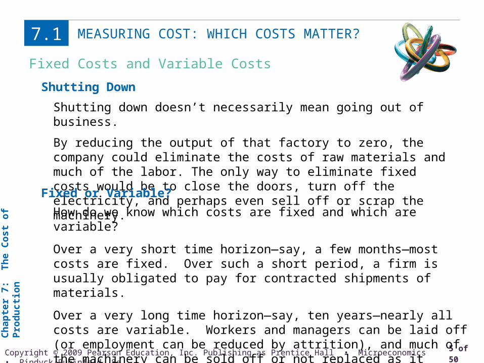
MEASURING COST: WHICH COSTS MATTER?7.1
Fixed Costs and Variable Costs
Shutting Down
Shutting down doesn’t necessarily mean going out of business.
By reducing the output of that factory to zero, the company could eliminate the costs of raw materials and much of the labor. The only way to eliminate fixed costs would be to close the doors, turn off the electricity, and perhaps even sell off or scrap the machinery.
Fixed or Variable?
How do we know which costs are fixed and which are variable?
Over a very short time horizon—say, a few months—most costs are fixed. Over such a short period, a firm is usually obligated to pay for contracted shipments of materials.
Over a very long time horizon—say, ten years—nearly all costs are variable. Workers and managers can be laid off (or employment can be reduced by attrition), and much of the machinery can be sold off or not replaced as it becomes obsolete and is scrapped.

Ch
apte
r 7:
T
he
Co
st
of
Pro
du
cti
on
6 of 50Copyright © 2009 Pearson Education, Inc. Publishing as Prentice Hall • Microeconomics • Pindyck/Rubinfeld, 8e.
MEASURING COST: WHICH COSTS MATTER?7.1
Fixed versus Sunk Costs
Amortizing Sunk Costs
●amortization Policy of treating a one-time expenditure as an annual cost spread out over some number of years.
Sunk costs are costs that have been incurred and cannot be recovered.
An example is the cost of R&D to a pharmaceutical company to develop and test a new drug and then, if the drug has been proven to be safe and effective, the cost of marketing it.
Whether the drug is a success or a failure, these costs cannot be recovered and thus are sunk.

Ch
apte
r 7:
T
he
Co
st
of
Pro
du
cti
on
7 of 50Copyright © 2009 Pearson Education, Inc. Publishing as Prentice Hall • Microeconomics • Pindyck/Rubinfeld, 8e.
MEASURING COST: WHICH COSTS MATTER?7.1
Marginal and Average Cost
Marginal Cost (MC)
●marginal cost (MC) Increase in cost resulting from the production of one extra unit of output.
Because fixed cost does not change as the firm’s level of output changes, marginal cost is equal to the increase in variable cost or the increase in total cost that results from an extra unit of output.
We can therefore write marginal cost as

Ch
apte
r 7:
T
he
Co
st
of
Pro
du
cti
on
8 of 50Copyright © 2009 Pearson Education, Inc. Publishing as Prentice Hall • Microeconomics • Pindyck/Rubinfeld, 8e.
MEASURING COST: WHICH COSTS MATTER?7.1
Marginal and Average Cost
TABLE 7.1 A Firm’s CostsRate of Fixed Variable Total Marginal Average Average AverageOutput Cost Cost Cost Cost Fixed Cost Variable Cost Total Cost(Units (Dollars (Dollars (Dollars (Dollars (Dollars (Dollars (Dollars
per Year) per Year) per Year) per Year) per Unit) per Unit) per Unit) per Unit)
(FC) (VC) (TC) (MC) (AFC) (AVC) (ATC)(1) (2) (3) (4) (5) (6) (7)
0 50 0 50 -- -- -- --
1 50 50 100 50 50 50 100
2 50 78 128 28 25 39 64
3 50 98 148 20 16.7 32.7 49.3
4 50 112 162 14 12.5 28 40.5
5 50 130 180 18 10 26 36
6 50 150 200 20 8.3 25 33.3
7 50 175 225 25 7.1 25 32.1
8 50 204 254 29 6.3 25.5 31.8
9 50 242 292 38 5.6 26.9 32.4
10 50 300 350 58 5 30 35
11 50 385 435 85 4.5 35 39.5
Marginal Cost (MC)

Ch
apte
r 7:
T
he
Co
st
of
Pro
du
cti
on
9 of 50Copyright © 2009 Pearson Education, Inc. Publishing as Prentice Hall • Microeconomics • Pindyck/Rubinfeld, 8e.
MEASURING COST: WHICH COSTS MATTER?7.1
Marginal and Average Cost
Average Total Cost (ATC)
●average total cost (ATC) Firm’s total cost divided by its level of output.
●average fixed cost (AFC) Fixed cost divided by the level of output.
●average variable cost (AVC) Variable cost divided by the level of output.
Ch
apte
r 7:
T
he
Co
st
of
Pro
du
cti
on
10 of 50Copyright © 2009 Pearson Education, Inc. Publishing as Prentice Hall • Microeconomics • Pindyck/Rubinfeld, 8e.
COST IN THE SHORT RUN7.2
The Determinants of Short-Run Cost
The change in variable cost is the per-unit cost of the extra labor w times the amount of extra labor needed to produce the extra output ΔL. Because ΔVC = wΔL, it follows that
The extra labor needed to obtain an extra unit of output is ΔL/Δq = 1/MPL. As a result,
(7.1)
Diminishing Marginal Returns and Marginal Cost
Diminishing marginal returns means that the marginal product of labor declines as the quantity of labor employed increases.
As a result, when there are diminishing marginal returns, marginal cost will increase as output increases.

Ch
apte
r 7:
T
he
Co
st
of
Pro
du
cti
on
11 of 50Copyright © 2009 Pearson Education, Inc. Publishing as Prentice Hall • Microeconomics • Pindyck/Rubinfeld, 8e.
COST IN THE SHORT RUN7.2
The Shapes of the Cost Curves
Cost Curves for a Firm
In (a) total cost TC is the vertical sum of fixed cost FC and variable cost VC.
In (b) average total cost ATC is the sum of average variable cost AVC and average fixed cost AFC.
Marginal cost MC crosses the average variable cost and average total cost curves at their minimum points.
Figure 7.1

Ch
apte
r 7:
T
he
Co
st
of
Pro
du
cti
on
12 of 50Copyright © 2009 Pearson Education, Inc. Publishing as Prentice Hall • Microeconomics • Pindyck/Rubinfeld, 8e.
COST IN THE SHORT RUN7.2
The Shapes of the Cost Curves
The Average-Marginal Relationship
Marginal and average costs are another example of the average-marginal relationship with respect to marginal and average product.
Total Cost as a Flow
Total cost is a flow—for example, some number of dollars per year. For simplicity, we will often drop the time reference, and refer to total cost in dollars and output in units.

Ch
apte
r 7:
T
he
Co
st
of
Pro
du
cti
on
13 of 50Copyright © 2009 Pearson Education, Inc. Publishing as Prentice Hall • Microeconomics • Pindyck/Rubinfeld, 8e.
COST IN THE LONG RUN7.3
The User Cost of Capital
●user cost of capital Annual cost of owning and using a capital asset, equal to economic depreciation plus forgone interest.
We can also express the user cost of capital as a rate per dollar of capital:
The user cost of capital is given by the sum of the economic depreciation and the interest (i.e., the financial return) that could have been earned had the money been invested elsewhere. Formally,

Ch
apte
r 7:
T
he
Co
st
of
Pro
du
cti
on
14 of 50Copyright © 2009 Pearson Education, Inc. Publishing as Prentice Hall • Microeconomics • Pindyck/Rubinfeld, 8e.
COST IN THE LONG RUN7.3
The Cost-Minimizing Input Choice
We now turn to a fundamental problem that all firms face: how to select inputs to produce a given output at minimum cost.
For simplicity, we will work with two variable inputs: labor (measured in hours of work per year) and capital (measured in hours of use of machinery per year).
The Price of CapitalThe price of capital is its user cost, given by r = Depreciation rate + Interest rate.
The Rental Rate of Capital
● rental rate Cost per year of renting one unit of capital.
If the capital market is competitive, the rental rate should be equal to the user cost, r. Why? Firms that own capital expect to earn a competitive return when they rent it. This competitive return is the user cost of capital.
Capital that is purchased can be treated as though it were rented at a rental rate equal to the user cost of capital.

Ch
apte
r 7:
T
he
Co
st
of
Pro
du
cti
on
15 of 50Copyright © 2009 Pearson Education, Inc. Publishing as Prentice Hall • Microeconomics • Pindyck/Rubinfeld, 8e.
COST IN THE LONG RUN7.3
The Isocost Line
(7.2)
● isocost line Graph showing all possible combinations of labor and capital that can be purchased for a given total cost.
To see what an isocost line looks like, recall that the total cost C of producing any particular output is given by the sum of the firm’s labor cost wL and its capital cost rK:

Ch
apte
r 7:
T
he
Co
st
of
Pro
du
cti
on
16 of 50Copyright © 2009 Pearson Education, Inc. Publishing as Prentice Hall • Microeconomics • Pindyck/Rubinfeld, 8e.
COST IN THE LONG RUN7.3
The Isocost Line
Producing a Given Output at Minimum Cost
Isocost curves describe the combination of inputs to production that cost the same amount to the firm.
Isocost curve C1 is tangent to isoquant q1 at A and shows that output q1 can be produced at minimum cost with labor input L1 and capital input K1.
Other input combinations-L2, K2 and L3, K3-yield the same output but at higher cost.
Figure 7.3

Ch
apte
r 7:
T
he
Co
st
of
Pro
du
cti
on
17 of 50Copyright © 2009 Pearson Education, Inc. Publishing as Prentice Hall • Microeconomics • Pindyck/Rubinfeld, 8e.
COST IN THE LONG RUN7.3
The Isocost Line
If we rewrite the total cost equation as an equation for a straight line, we get
It follows that the isocost line has a slope of ΔK/ΔL = −(w/r), which is the ratio of the wage rate to the rental cost of capital.

Ch
apte
r 7:
T
he
Co
st
of
Pro
du
cti
on
18 of 50Copyright © 2009 Pearson Education, Inc. Publishing as Prentice Hall • Microeconomics • Pindyck/Rubinfeld, 8e.
COST IN THE LONG RUN7.3
Choosing Inputs
Input Substitution When an Input Price Changes
Facing an isocost curve C1, the firm produces output q1 at point A using L1 units of labor and K1 units of capital.
When the price of labor increases, the isocost curves become steeper.
Output q1 is now produced at point B on isocost curve C2 by using L2 units of labor and K2 units of capital.
Figure 7.4
Ch
apte
r 7:
T
he
Co
st
of
Pro
du
cti
on
19 of 50Copyright © 2009 Pearson Education, Inc. Publishing as Prentice Hall • Microeconomics • Pindyck/Rubinfeld, 8e.
COST IN THE LONG RUN7.3
Choosing Inputs
(7.3)
Recall that in our analysis of production technology, we showed that the marginal rate of technical substitution of labor for capital (MRTS) is the negative of the slope of the isoquant and is equal to the ratio of the marginal products of labor and capital:
It follows that when a firm minimizes the cost of producing a particular output, the following condition holds:
We can rewrite this condition slightly as follows:
(7.4)

Ch
apte
r 7:
T
he
Co
st
of
Pro
du
cti
on
20 of 50Copyright © 2009 Pearson Education, Inc. Publishing as Prentice Hall • Microeconomics • Pindyck/Rubinfeld, 8e.
COST IN THE LONG RUN7.3
Cost Minimization with Varying Output Levels
● expansion path Curve passing through points of tangency between a firm’s isocost lines and its isoquants.
The Expansion Path and Long-Run Costs
To move from the expansion path to the cost curve, we follow three steps:
1. Choose an output level represented by an isoquant. Then find the point of tangency of that isoquant with an isocost line.
2. From the chosen isocost line determine the minimum cost of producing the output level that has been selected.
3. Graph the output-cost combination.

Ch
apte
r 7:
T
he
Co
st
of
Pro
du
cti
on
21 of 50Copyright © 2009 Pearson Education, Inc. Publishing as Prentice Hall • Microeconomics • Pindyck/Rubinfeld, 8e.
COST IN THE LONG RUN7.3
Cost Minimization with Varying Output Levels
Input Substitution When an Input Price Changes
In (a), the expansion path (from the origin through points A, B, and C) illustrates the lowest-cost combinations of labor and capital that can be used to produce each level of output in the long run— i.e., when both inputs to production can be varied.
In (b), the corresponding long-run total cost curve (from the origin through points D, E, and F) measures the least cost of producing each level of output.
Figure 7.6

Ch
apte
r 7:
T
he
Co
st
of
Pro
du
cti
on
22 of 50Copyright © 2009 Pearson Education, Inc. Publishing as Prentice Hall • Microeconomics • Pindyck/Rubinfeld, 8e.
LONG-RUN VERSUS SHORT-RUN COST CURVES7.4
The Inflexibility of Short-Run Production
The Inflexibility of Short-Run Production
When a firm operates in the short run, its cost of production may not be minimized because of inflexibility in the use of capital inputs.
Output is initially at level q1, (using L1, K1).
In the short run, output q2 can be produced only by increasing labor from L1 to L3 because capital is fixed at K1.
In the long run, the same output can be produced more cheaply by increasing labor from L1 to L2 and capital from K1 to K2.
Figure 7.7

Ch
apte
r 7:
T
he
Co
st
of
Pro
du
cti
on
23 of 50Copyright © 2009 Pearson Education, Inc. Publishing as Prentice Hall • Microeconomics • Pindyck/Rubinfeld, 8e.
LONG-RUN VERSUS SHORT-RUN COST CURVES7.4
Long-Run Average Cost
Long-Run Average and Marginal Cost
When a firm is producing at an output at which the long-run average cost LAC is falling, the long-run marginal cost LMC is less than LAC.
Conversely, when LAC is increasing, LMC is greater than LAC.
The two curves intersect at A, where the LAC curve achieves its minimum.
Figure 7.8

Ch
apte
r 7:
T
he
Co
st
of
Pro
du
cti
on
24 of 50Copyright © 2009 Pearson Education, Inc. Publishing as Prentice Hall • Microeconomics • Pindyck/Rubinfeld, 8e.
LONG-RUN VERSUS SHORT-RUN COST CURVES7.4
Long-Run Average Cost
● long-run average cost curve (LAC) Curve relating average cost of production to output when all inputs, including capital, are variable.
● short-run average cost curve (SAC) Curve relating average cost of production to output when level of capital is fixed.
● long-run marginal cost curve (LMC) Curve showing the change in long-run total cost as output is increased incrementally by 1 unit.
Ch
apte
r 7:
T
he
Co
st
of
Pro
du
cti
on
25 of 50Copyright © 2009 Pearson Education, Inc. Publishing as Prentice Hall • Microeconomics • Pindyck/Rubinfeld, 8e.
LONG-RUN VERSUS SHORT-RUN COST CURVES7.4
Economies and Diseconomies of Scale
As output increases, the firm’s average cost of producing that output is likely to decline, at least to a point.
This can happen for the following reasons:
1. If the firm operates on a larger scale, workers can specialize in the activities at which they are most productive.
2. Scale can provide flexibility. By varying the combination of inputs utilized to produce the firm’s output, managers can organize the production process more effectively.
3. The firm may be able to acquire some production inputs at lower cost because it is buying them in large quantities and can therefore negotiate better prices. The mix of inputs might change with the scale of the firm’s operation if managers take advantage of lower-cost inputs.
Ch
apte
r 7:
T
he
Co
st
of
Pro
du
cti
on
26 of 50Copyright © 2009 Pearson Education, Inc. Publishing as Prentice Hall • Microeconomics • Pindyck/Rubinfeld, 8e.
LONG-RUN VERSUS SHORT-RUN COST CURVES7.4
Economies and Diseconomies of Scale
At some point, however, it is likely that the average cost of production will begin to increase with output.
There are three reasons for this shift:
1. At least in the short run, factory space and machinery may make it more difficult for workers to do their jobs effectively.
2. Managing a larger firm may become more complex and inefficient as the number of tasks increases.
3. The advantages of buying in bulk may have disappeared once certain quantities are reached. At some point, available supplies of key inputs may be limited, pushing their costs up.

Ch
apte
r 7:
T
he
Co
st
of
Pro
du
cti
on
27 of 50Copyright © 2009 Pearson Education, Inc. Publishing as Prentice Hall • Microeconomics • Pindyck/Rubinfeld, 8e.
LONG-RUN VERSUS SHORT-RUN COST CURVES7.4
Economies and Diseconomies of Scale
● economies of scale Situation in which output can be doubled for less than a doubling of cost.
● diseconomies of scale Situation in which a doubling of output requires more than a doubling of cost.
Increasing Returns to Scale: Output more than doubles when the quantities of all inputs are doubled.
Economies of Scale: A doubling of output requires less than a doubling of cost.
Ch
apte
r 7:
T
he
Co
st
of
Pro
du
cti
on
28 of 50Copyright © 2009 Pearson Education, Inc. Publishing as Prentice Hall • Microeconomics • Pindyck/Rubinfeld, 8e.
LONG-RUN VERSUS SHORT-RUN COST CURVES7.4
Economies and Diseconomies of Scale
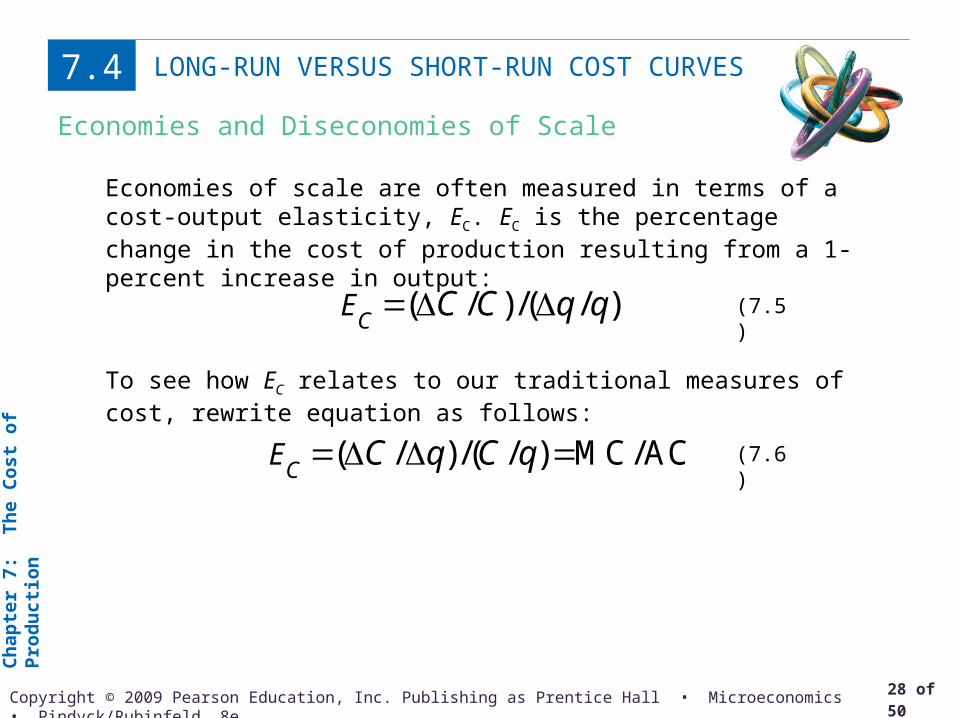
Economies of scale are often measured in terms of a cost-output elasticity, EC. EC is the percentage change in the cost of production resulting from a 1-percent increase in output:
(7.5)
To see how EC relates to our traditional measures of cost, rewrite equation as follows:
(7.6)( / )/( / ) MC/ACCE C q C q
( / )/( / )CE C C q q
Ch
apte
r 7:
T
he
Co
st
of
Pro
du
cti
on
29 of 50Copyright © 2009 Pearson Education, Inc. Publishing as Prentice Hall • Microeconomics • Pindyck/Rubinfeld, 8e.
LONG-RUN VERSUS SHORT-RUN COST CURVES7.4
The Relationship Between Short-Run and Long-Run Cost
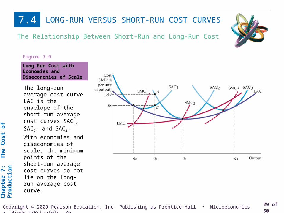
Long-Run Cost with Economies and Diseconomies of Scale
The long-run average cost curve LAC is the envelope of the short-run average cost curves SAC1, SAC2, and SAC3.
With economies and diseconomies of scale, the minimum points of the short-run average cost curves do not lie on the long-run average cost curve.
Figure 7.9
Ch
apte
r 7:
T
he
Co
st
of
Pro
du
cti
on
30 of 50Copyright © 2009 Pearson Education, Inc. Publishing as Prentice Hall • Microeconomics • Pindyck/Rubinfeld, 8e.
PRODUCTION WITH TWO OUTPUTS—ECONOMIES OF SCOPE
7.5
Product Transformation Curves
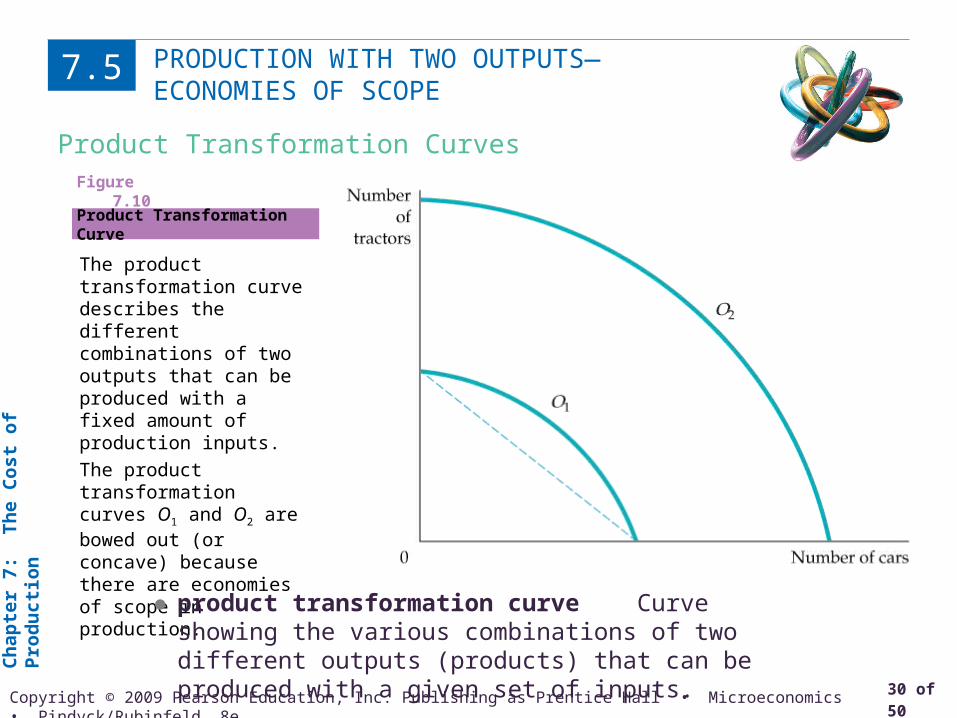
Product Transformation Curve
The product transformation curve describes the different combinations of two outputs that can be produced with a fixed amount of production inputs.
The product transformation curves O1 and O2 are bowed out (or concave) because there are economies of scope in production.
Figure 7.10
● product transformation curve Curve showing the various combinations of two different outputs (products) that can be produced with a given set of inputs.
Ch
apte
r 7:
T
he
Co
st
of
Pro
du
cti
on
31 of 50Copyright © 2009 Pearson Education, Inc. Publishing as Prentice Hall • Microeconomics • Pindyck/Rubinfeld, 8e.
PRODUCTION WITH TWO OUTPUTS—ECONOMIES OF SCOPE
7.5
Economies and Diseconomies of Scope
● economies of scope Situation in which joint output of a single firm is greater than output that could be achieved by two different firms when each produces a single product.
● diseconomies of scope Situation in which joint output of a single firm is less than could be achieved by separate firms when each produces a single product.

Ch
apte
r 7:
T
he
Co
st
of
Pro
du
cti
on
32 of 50Copyright © 2009 Pearson Education, Inc. Publishing as Prentice Hall • Microeconomics • Pindyck/Rubinfeld, 8e.
PRODUCTION WITH TWO OUTPUTS—ECONOMIES OF SCOPE
7.5
The Degree of Economies of Scope
● degree of economies of scope (SC) Percentage of cost savings resulting when two or more products are produced jointly rather than Individually.
To measure the degree to which there are economies of scope, we should ask what percentage of the cost of production is saved when two (or more) products are produced jointly rather than individually.
(7.7)
Ch
apte
r 7:
T
he
Co
st
of
Pro
du
cti
on
33 of 50Copyright © 2009 Pearson Education, Inc. Publishing as Prentice Hall • Microeconomics • Pindyck/Rubinfeld, 8e.
DYNAMIC CHANGES IN COSTS—THE LEARNING CURVE
7.6
As management and labor gain experience with production, the firm’s marginal and average costs of producing a given level of output fall for four reasons:
1. Workers often take longer to accomplish a given task the first few times they do it. As they become more adept, their speed increases.
2. Managers learn to schedule the production process more effectively, from the flow of materials to the organization of the manufacturing itself.
3. Engineers who are initially cautious in their product designs may gain enough experience to be able to allow for tolerances in design that save costs without increasing defects. Better and more specialized tools and plant organization may also lower cost.
4. Suppliers may learn how to process required materials more effectively and pass on some of this advantage in the form of lower costs.

Ch
apte
r 7:
T
he
Co
st
of
Pro
du
cti
on
34 of 50Copyright © 2009 Pearson Education, Inc. Publishing as Prentice Hall • Microeconomics • Pindyck/Rubinfeld, 8e.
DYNAMIC CHANGES IN COSTS—THE LEARNING CURVE
7.6
The Learning Curve
A firm’s production cost may fall over time as managers and workers become more experienced and more effective at using the available plant and equipment.
The learning curve shows the extent to which hours of labor needed per unit of output fall as the cumulative output increases.
Figure 7.11
● learning curve Graph relating amount of inputs needed by a firm to produce each unit of output to its cumulative output.
Related Documents