1 Chapter 7 Packet-Switching Networks Networks Network Services and Internal Network Operation Packet Network Topology Datagrams and Virtual Circuits Routing in Packet Networks Shortest Path Routing ATM Networks Traffic Management Network Layer Network Layer: the most complex layer Requires the coordinated actions of multiple Requires the coordinated actions of multiple, geographically distributed network elements (switches & routers) Must be able to deal with very large scales Billions of users (people & communicating devices) Biggest Challenges Addressing: where should information be directed to? Routing: what path should be used to get information there?

Welcome message from author
This document is posted to help you gain knowledge. Please leave a comment to let me know what you think about it! Share it to your friends and learn new things together.
Transcript

1
Chapter 7Packet-Switching
NetworksNetworks
Network Services and Internal Network OperationPacket Network Topology
Datagrams and Virtual CircuitsRouting in Packet Networksg
Shortest Path RoutingATM Networks
Traffic Management
Network Layer
Network Layer: the most complex layer Requires the coordinated actions of multiple Requires the coordinated actions of multiple,
geographically distributed network elements (switches & routers)
Must be able to deal with very large scales Billions of users (people & communicating devices)
Biggest Challengesgg g Addressing: where should information be directed to?
Routing: what path should be used to get information there?
2
t0t1
Packet Switching
Network
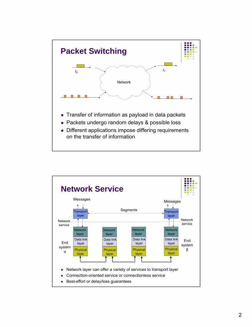
Transfer of information as payload in data packets Transfer of information as payload in data packets
Packets undergo random delays & possible loss
Different applications impose differing requirements on the transfer of information
Transport Transport
MessagesMessages
Segments
Network Service
End system
βPhysical
Data linklayer
Physical
Data linklayerEnd
system
Networklayer
Networklayer
Physical
Data linklayer
Networklayer
Physical
Data linklayer
Networklayer
player
Transportlayer
Networkservice
Networkservice
βPhysicallayer
Physicallayerα Physical
layerPhysical
layer
Network layer can offer a variety of services to transport layer
Connection-oriented service or connectionless service
Best-effort or delay/loss guarantees
3
Network Service vs. Operation
Network Service
Connectionless
Internal Network Operation
Datagram Transfer
Connection-Oriented Reliable and possibly
constant bit rate transfer
Connectionless IP
Connection-Oriented Telephone connection
ATM
Various combinations are possible Connection-oriented service over Connectionless operation
Connectionless service over Connection-Oriented operation
Context & requirements determine what makes sense
Network Layer Functions
What are essentials?
Routing: mechanisms for determining the set of Routing: mechanisms for determining the set of best paths for routing packets requires the collaboration of network elements
Forwarding: transfer of packets from NE inputs to outputs
Priority & Scheduling: determining order of Priority & Scheduling: determining order of packet transmission in each NEOptional: congestion control, segmentation & reassembly, security
4
End-to-End Packet Network
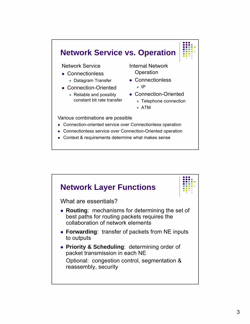
Packet networks very different than telephone networks
Individual packet streams are highly bursty Statistical multiplexing is used to concentrate streams
User demand can undergo dramatic change Peer-to-peer applications stimulated huge growth in traffic
volumes
I t t t t hi hl d t li d Internet structure highly decentralized Paths traversed by packets can go through many networks
controlled by different organizations
No single entity responsible for end-to-end service
Access Multiplexing
AccessMUX
Topacketnetwork
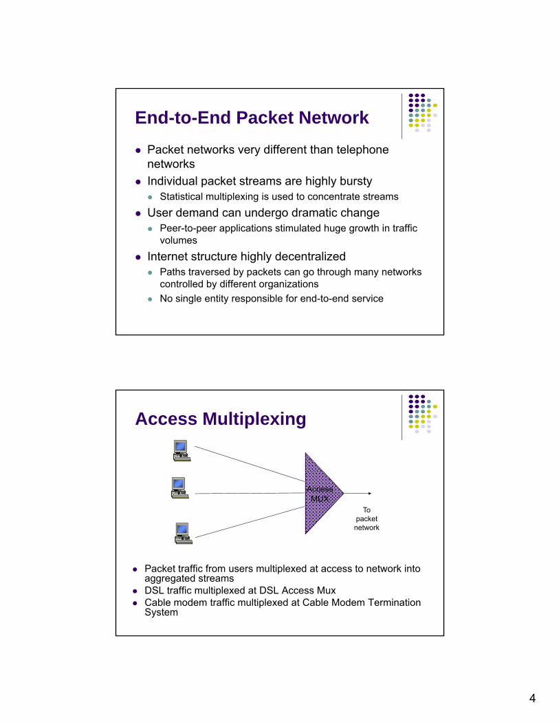
Packet traffic from users multiplexed at access to network into aggregated streams
DSL traffic multiplexed at DSL Access Mux Cable modem traffic multiplexed at Cable Modem Termination
System
5
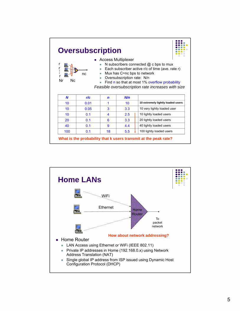
Oversubscription Access Multiplexer
N subscribers connected @ c bps to mux Each subscriber active r/c of time (ave. rate r) Mux has C=nc bps to network•
• •
rr
nc • •
Mux has C=nc bps to network Oversubscription rate: N/n Find n so that at most 1% overflow probability
Feasible oversubscription rate increases with size
N r/c n N/n
10 0.01 1 10 10 extremely lightly loaded users
10 0 05 3 3 3 10 very lightly loaded user
Nr Ncr nc•
10 0.05 3 3.3 10 very lightly loaded user
10 0.1 4 2.5 10 lightly loaded users
20 0.1 6 3.3 20 lightly loaded users
40 0.1 9 4.4 40 lightly loaded users
100 0.1 18 5.5 100 lightly loaded users
What is the probability that k users transmit at the peak rate?
Home LANs
WiFi
HomeRouter
Topacketnetwork
Ethernet
How about network addressing? Home Router
LAN Access using Ethernet or WiFi (IEEE 802.11) Private IP addresses in Home (192.168.0.x) using Network
Address Translation (NAT) Single global IP address from ISP issued using Dynamic Host
Configuration Protocol (DHCP)
6
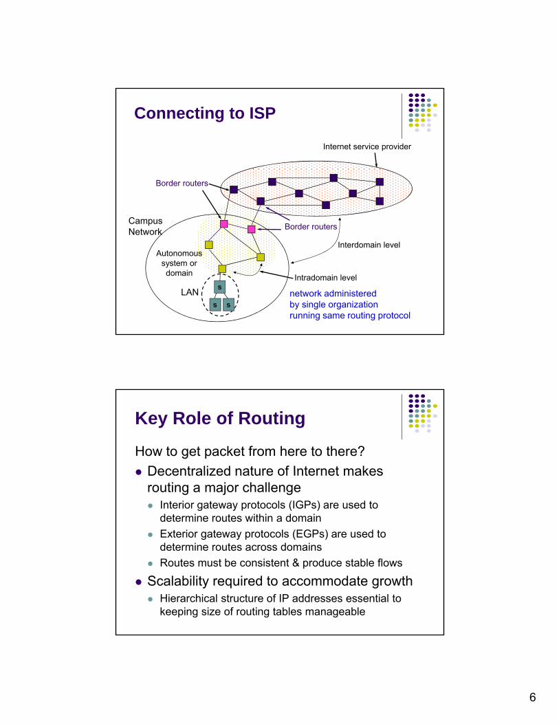
Internet service provider
Connecting to ISP
Interdomain levelAutonomous
Border routers
Border routers
CampusNetwork
Intradomain level
Autonomoussystem ordomain
s
ss
LAN network administeredby single organizationrunning same routing protocol
Key Role of Routing
How to get packet from here to there?
Decentralized nature of Internet makes Decentralized nature of Internet makes routing a major challenge Interior gateway protocols (IGPs) are used to
determine routes within a domain
Exterior gateway protocols (EGPs) are used to determine routes across domains
Routes must be consistent & produce stable flows
Scalability required to accommodate growth Hierarchical structure of IP addresses essential to
keeping size of routing tables manageable

7
Chapter 7Packet-Switching
NetworksNetworks
Datagrams and Virtual Circuits
User
Packet Switching Network
Packet switching network Transfers packets
Packetswitch
Network
Transmissionline
User Transfers packets between users
Transmission lines + packet switches (routers)
Origin in message switchingswitching
Two modes of operation: Connectionless Virtual Circuit

8
Message switching invented for telegraphy
Message Switching
Entire messages multiplexed onto shared lines, stored & forwarded
Headers for source & destination addresses
Routing at message switches
Message
Source
Message
Message
Message
ConnectionlessSwitches Destination
Transmission delay vs. propagation delay Transmit a 1000B from LA to DC via a 1Gbps network,
signal speed 200Km/sec.
tSource T
Message Switching Delay
t
t
t
t
Destination
Switch 1
Switch 2
Delay
Minimum delay = 3 + 3T
Additional queueing delays possible at each link
9
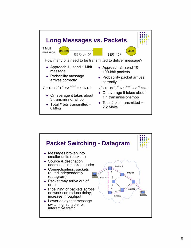
Long Messages vs. Packets1 Mbit message source dest
BER=p=10-6 BER=10-6
Approach 1: send 1 Mbit message
Probability message arrives correctly
How many bits need to be transmitted to deliver message?
Approach 2: send 10 100-kbit packets
Probability packet arrives correctly
/)( 11010106 666 101010106 655
On average it takes about 3 transmissions/hop
Total # bits transmitted ≈ 6 Mbits
On average it takes about 1.1 transmissions/hop
Total # bits transmitted ≈ 2.2 Mbits
3/1)101( 11010106 eePc 9.0)101( 1.01010106 655
eePc
Packet Switching - Datagram
Messages broken into smaller units (packets)
Source & destination Source & destination addresses in packet header
Connectionless, packets routed independently (datagram)
Packet may arrive out of order
Pipelining of packets across
Packet 2
Packet 1
Packet 1
Packet 2 Pipelining of packets across network can reduce delay, increase throughput
Lower delay that message switching, suitable for interactive traffic
Packet 2
Packet 2
10
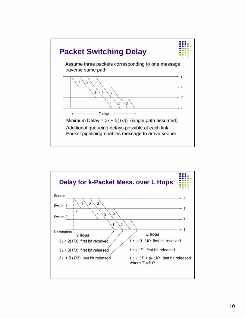
Packet Switching Delay
Assume three packets corresponding to one message traverse same path
t
t
t
t
31 2
31 2
321
Delay
Minimum Delay = 3τ + 5(T/3) (single path assumed)
Additional queueing delays possible at each linkPacket pipelining enables message to arrive sooner
t
t321
Source
Switch 1
Delay for k-Packet Mess. over L Hops
t
t
t31 2
31 2
3 + 2(T/3) first bit received L + (L-1)P first bit received3 hops L hops
Destination
Switch 1
Switch 2
( )
3 + 3(T/3) first bit released
3 + 5 (T/3) last bit released
L + LP first bit released
L + LP + (k-1)P last bit releasedwhere T = k P

11
Destination
address
Output
port
Routing Tables in Datagram Networks
Route determined by table lookup
1345 12
70785
61566
lookup
Routing decision involves finding next hop in route to given destination
Routing table has an entry for each destination specifying output port that
2458 12
leads to next hop
Size of table becomes impractical for very large number of destinations
Example: Internet Routing
Internet protocol uses datagram packet switching across networks Networks are treated as data links
Hosts have two-part IP address: Network address + Host address
Routers do table lookup on network address This reduces size of routing tableg
In addition, network addresses are assigned so that they can also be aggregated Discussed as CIDR in Chapter 8

12
Packet Switching – Virtual Circuit
Packet Packet
Packet
Call set-up phase sets ups pointers in fixed path along network
All packets for a connection follow the same path
Virtual circuit
Packet
All packets for a connection follow the same path
Abbreviated header identifies connection on each link
Packets queue for transmission
Variable bit rates possible, negotiated during call set-up
Delays variable, cannot be less than circuit switching
ATM Virtual Circuits
A VC is a connection with resources reserved.
A Cell is a small and fixed-size packet, delivered in order.

13
Routing in VC Subnet
Label switching
Does VC subnets need the capability to route isolated packets from an arbitrary source to an arbitrary destination?
SW SW SW
Connect request
Connect request
Connect request
…
Connection Setup
1 2 nConnect confirm
Connect confirm
Connect confirm
…
Signaling messages propagate as route is selected
Signaling messages identify connection and setup tables in switches
Typically a connection is identified by a local tag, Virtual Circuit Identifier (VCI)
Each switch only needs to know how to relate an incoming tag in one input to an outgoing tag in the corresponding output
Once tables are setup, packets can flow along path
14
t321
Connect request CC
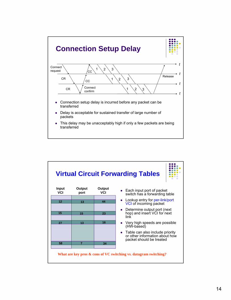
Connection Setup Delay
t
t
t31 2
31 2
Release
request
CR
CR Connect confirm
CC
CC
Connection setup delay is incurred before any packet can be transferred
Delay is acceptable for sustained transfer of large number of packets
This delay may be unacceptably high if only a few packets are being transferred
InputVCI
Outputport
OutputVCI
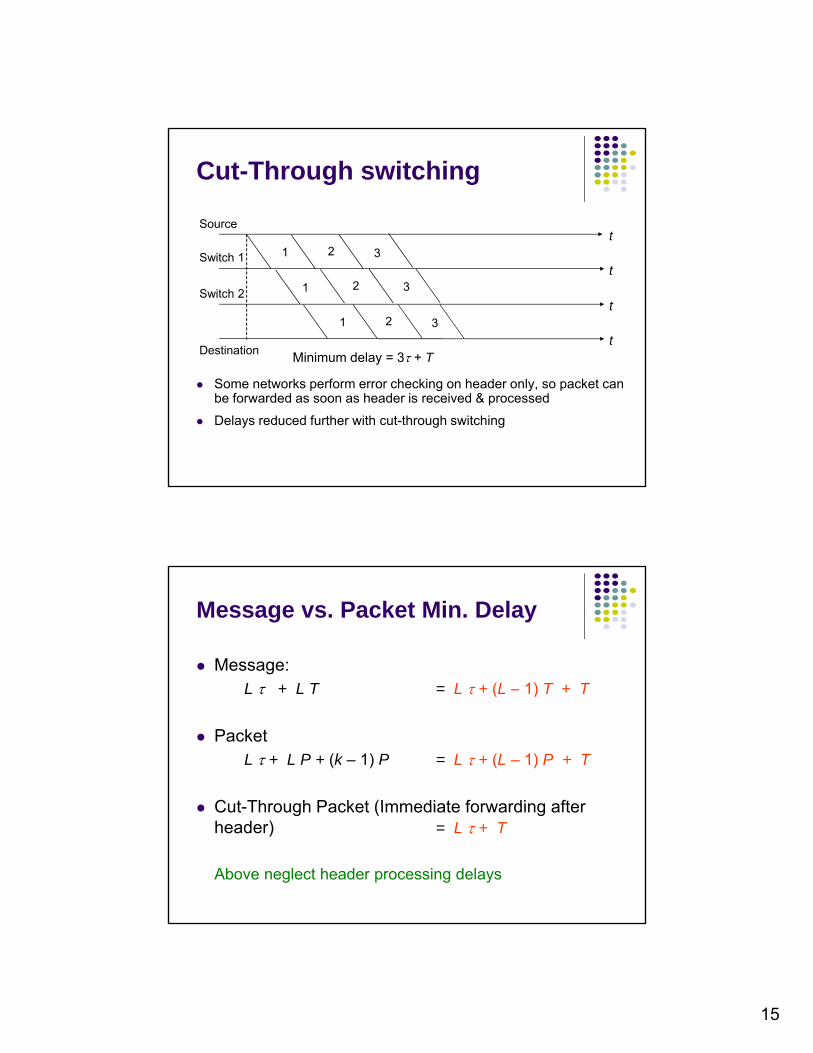
Virtual Circuit Forwarding Tables
Each input port of packet switch has a forwarding table
15 15
13
1327
12 44
23
16
switch has a forwarding table
Lookup entry for per-link/port VCI of incoming packet
Determine output port (next hop) and insert VCI for next link
Very high speeds are possible (HW-based)
58 7 34
Table can also include priority or other information about how packet should be treated
What are key pros & cons of VC switching vs. datagram switching?
15
21t
Source
Cut-Through switching
31 2
31 2
321
Minimum delay = 3 + Tt
t
t
Destination
Switch 1
Switch 2
Some networks perform error checking on header only, so packet can be forwarded as soon as header is received & processed
Delays reduced further with cut-through switching
Message vs. Packet Min. Delay
Message:L + L T L + (L 1) T + TL + L T = L + (L – 1) T + T
PacketL + L P + (k – 1) P = L + (L – 1) P + T
Cut Through Packet (Immediate forwarding after Cut-Through Packet (Immediate forwarding after header) = L + T
Above neglect header processing delays
16
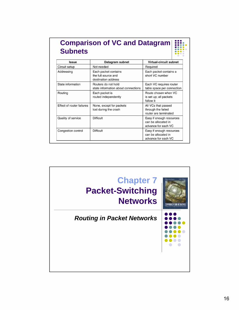
Comparison of VC and Datagram Subnets
5-4
Chapter 7Packet-Switching
NetworksNetworks
Routing in Packet Networks

17
1 36
Routing in Packet Networks
2
4
5 Node (switch or router)
Three possible (loopfree) routes from 1 to 6: 1-3-6, 1-4-5-6, 1-2-5-6
Which is “best”? Min delay? Min hop? Max bandwidth? Min cost?
Max reliability?
What is the objective function for optimization?
Creating the Routing Tables
Need information on state of links Link up/down; congested; delay or other metrics Link up/down; congested; delay or other metrics
Need to distribute link state information using a routing protocol What information is exchanged? How often?
How to exchange with neighbors?
f Need to compute routes based on information Single metric; multiple metrics
Single route; alternate routes
18
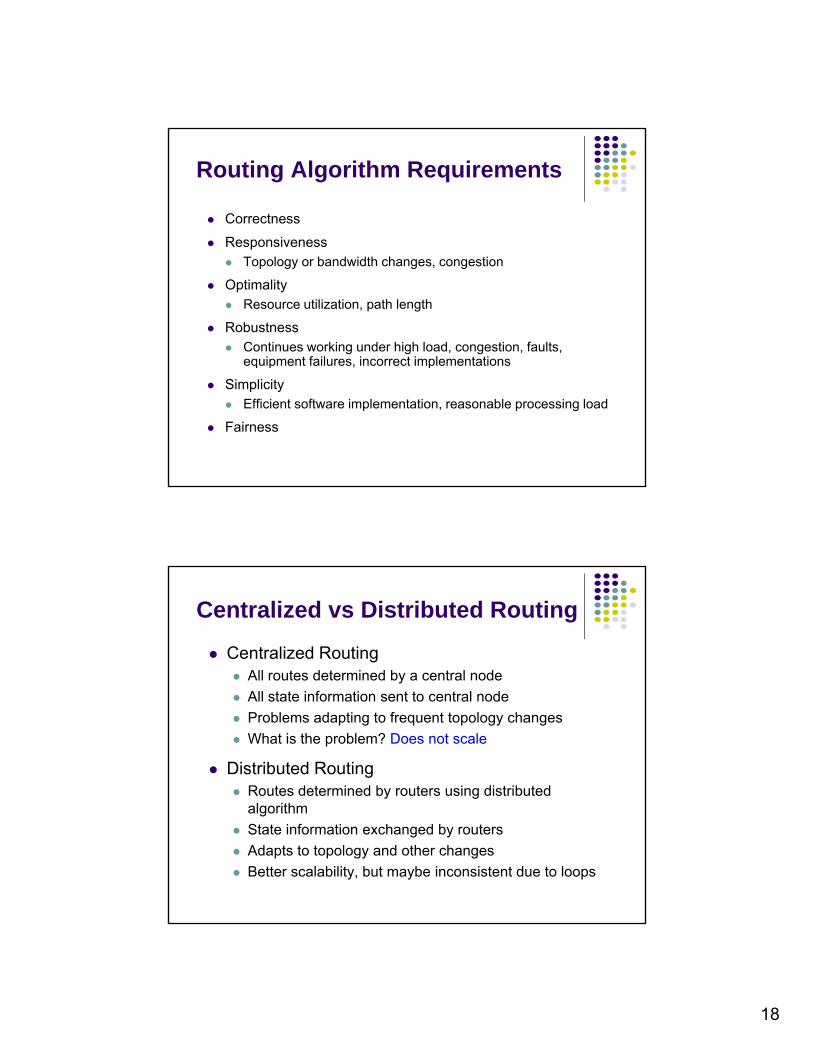
Routing Algorithm Requirements
Correctness
Responsivenessp Topology or bandwidth changes, congestion
Optimality Resource utilization, path length
Robustness Continues working under high load, congestion, faults,
equipment failures, incorrect implementationsq p , p
Simplicity Efficient software implementation, reasonable processing load
Fairness
Centralized vs Distributed Routing
Centralized Routing All routes determined by a central node
All state information sent to central node
Problems adapting to frequent topology changes
What is the problem? Does not scale
Distributed Routing Routes determined by routers using distributed
l ithalgorithm
State information exchanged by routers
Adapts to topology and other changes
Better scalability, but maybe inconsistent due to loops

19
Static vs Dynamic Routing
Static Routing Set up manually, do not change; requires administrationy g
Works when traffic predictable & network is simple
Used to override some routes set by dynamic algorithm
Used to provide default router
Dynamic Routing Adapt to changes in network conditions
Automated
Calculates routes based on received updated network state information
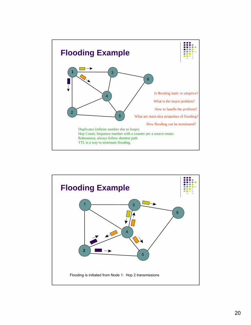
Flooding
Send a packet to all nodes in a network Useful in starting up network or broadcast
No routing tables available
Need to broadcast packet to all nodes (e.g. to propagate link state information)
A hApproach Send packet on all ports except one where it arrived
Exponential growth in packet transmissions
20
1 3
Flooding Example
2
4
6
Is flooding static or adaptive?
What is the major problem?
How to handle the problem?2
5 What are main nice properties of flooding?
Duplicates (infinite number due to loops)Hop Count; Sequence number with a counter per a source router.Robustness; always follow shortest pathTTL is a way to terminate flooding.
How flooding can be terminated?
1 3
6
Flooding Example
4
6
25
Flooding is initiated from Node 1: Hop 2 transmissions
21
1 3
6
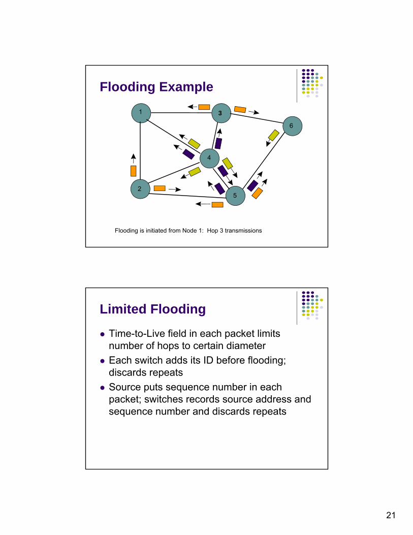
Flooding Example
2
4
6
25
Flooding is initiated from Node 1: Hop 3 transmissions
Limited Flooding
Time-to-Live field in each packet limits number of hops to certain diameternumber of hops to certain diameter
Each switch adds its ID before flooding; discards repeats
Source puts sequence number in each packet; switches records source address and
b d di d tsequence number and discards repeats
22
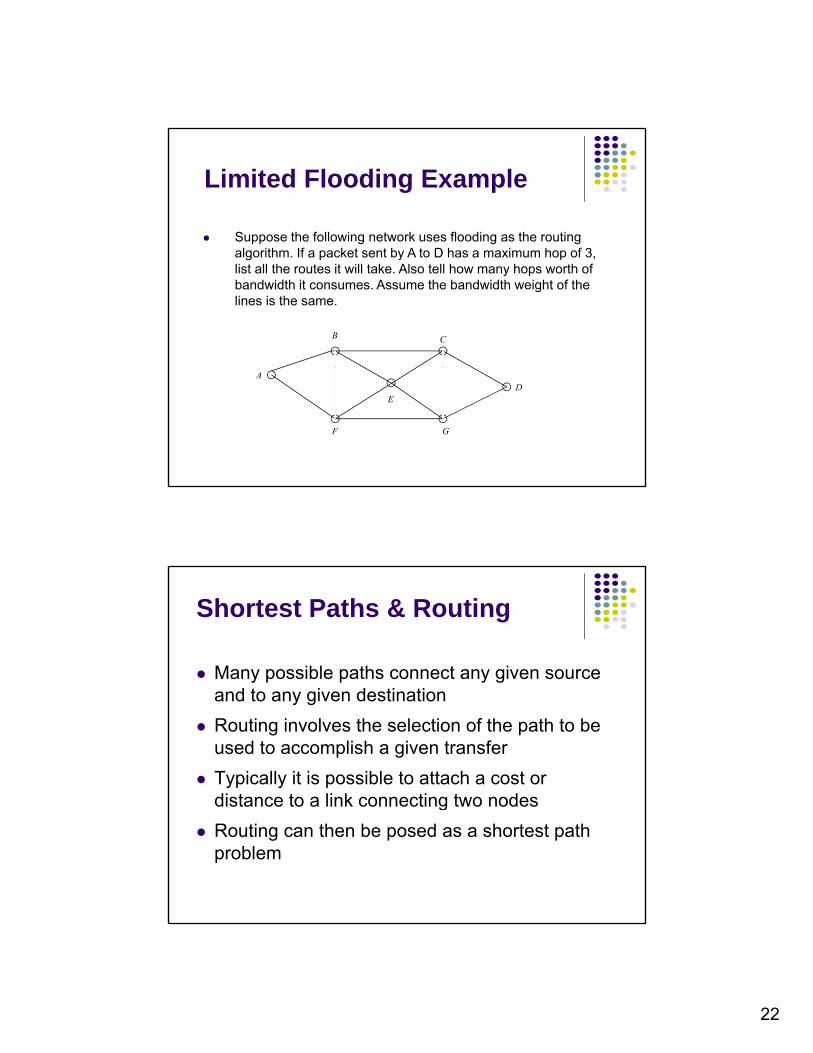
Suppose the following network uses flooding as the routing
Limited Flooding Example
CB
algorithm. If a packet sent by A to D has a maximum hop of 3, list all the routes it will take. Also tell how many hops worth of bandwidth it consumes. Assume the bandwidth weight of the lines is the same.
A
ED
F G
Shortest Paths & Routing
Many possible paths connect any given source and to any given destination
Routing involves the selection of the path to be used to accomplish a given transfer
Typically it is possible to attach a cost or distance to a link connecting two nodesdistance to a link connecting two nodes
Routing can then be posed as a shortest path problem
23
Routing Metrics
Means for measuring desirability of a path
Path Length = sum of costs or distancesPath Length sum of costs or distances
Possible metrics Hop count: rough measure of resources used
Reliability: link availability
Delay: sum of delays along path; complex & dynamic
Bandwidth: “available capacity” in a path
Load: Link & router utilization along path
Cost: $$$
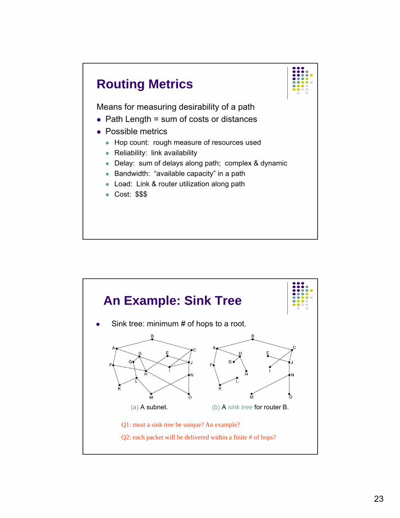
An Example: Sink Tree
Sink tree: minimum # of hops to a root.
Q1: must a sink tree be unique? An example?
Q2: each packet will be delivered within a finite # of hops?
(a) A subnet. (b) A sink tree for router B.
24
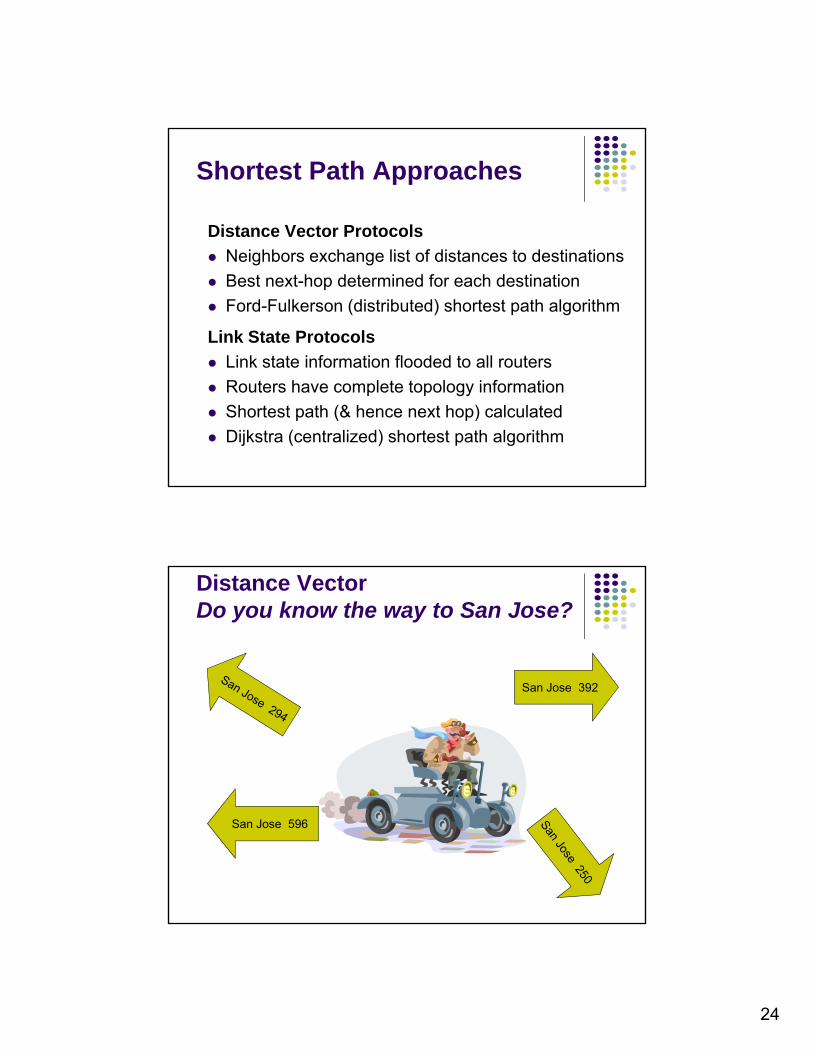
Shortest Path Approaches
Distance Vector Protocols
Neighbors exchange list of distances to destinations
Best next-hop determined for each destination
Ford-Fulkerson (distributed) shortest path algorithm
Link State Protocols
Link state information flooded to all routersLink state information flooded to all routers
Routers have complete topology information
Shortest path (& hence next hop) calculated
Dijkstra (centralized) shortest path algorithm
S J 392
Distance VectorDo you know the way to San Jose?
San Jose 392
San Jose 596
25
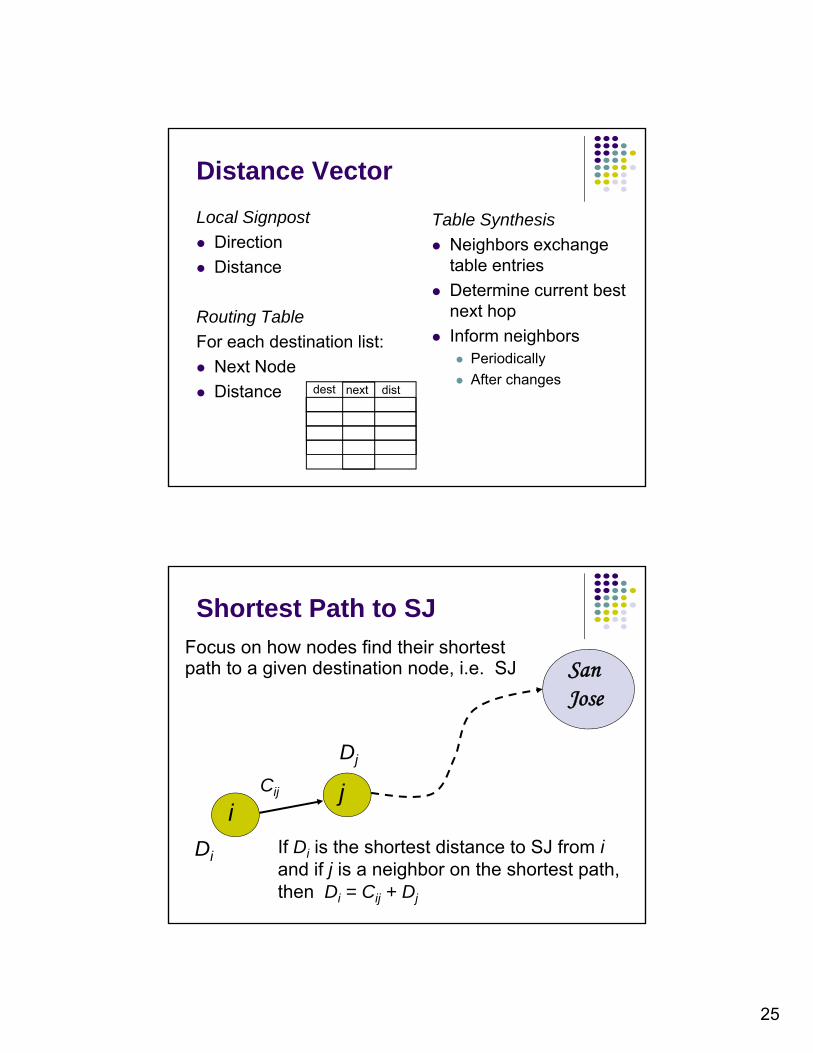
Distance Vector
Local Signpost
DirectionTable Synthesis
Neighbors exchangeDirection
Distance
Routing Table
For each destination list:
Next Node
Neighbors exchange table entries
Determine current best next hop
Inform neighbors Periodically
Next Node
Distance After changes
dest next dist
Shortest Path to SJ
SanFocus on how nodes find their shortest path to a given destination node, i.e. SJ
ij
Jose
Cij
Dj
ij
Di If Di is the shortest distance to SJ from iand if j is a neighbor on the shortest path, then Di = Cij + Dj
26
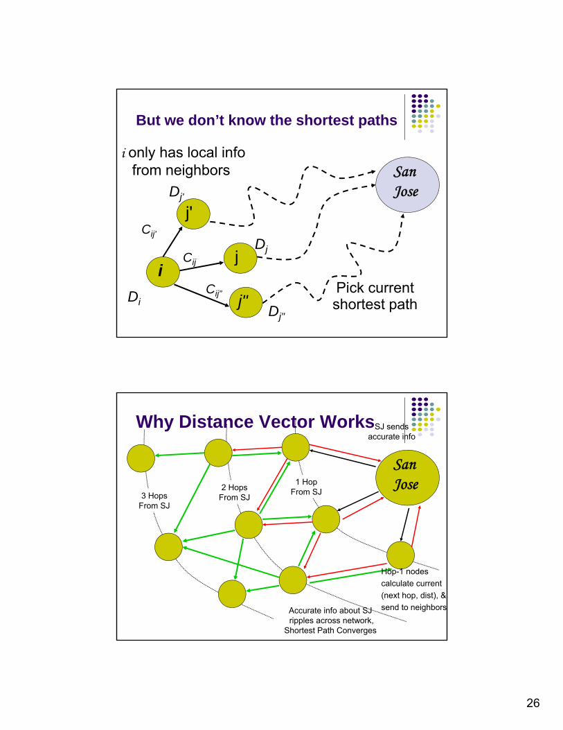
i only has local infofrom neighbors San
But we don’t know the shortest paths
from neighbors SanJose
jCDj
Cij'
j'Dj'
Dj"
Cij”
ijCij
Di j"Pick current shortest path
Why Distance Vector Works
San
SJ sendsaccurate info
Jose1 HopFrom SJ2 Hops
From SJ3 HopsFrom SJ
Accurate info about SJripples across network,
Shortest Path Converges
Hop-1 nodes
calculate current
(next hop, dist), &
send to neighbors

27
Distance Vector Routing (RIP)
Routing operates by having each router maintain a vector table giving the best known distance to each destination and which line to use to get there. The tables are updated by exchanging information with the neighbors.
Vector table: one entry for each router in the subnet; each entry contains two parts: preferred outgoing line to use for that destination and an estimate of the time or distance to the destination.
The router is assumed to know the distance/cost to each neighbor and update the vector table periodically by changing it with neighbors.
# hops
Delay (ECHO)
Capacity
Congestion
mX i
An Example
(a) A subnet. (b) Input from A, I, H, K, and the new routing table for J.
28
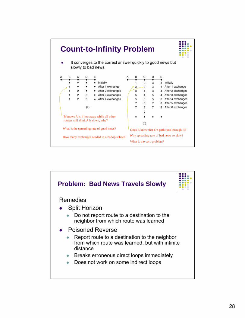
Count-to-Infinity Problem
It converges to the correct answer quickly to good news but slowly to bad news.
B knows A is 1 hop away while all otherrouters still think A is down, why?
What is the spreading rate of good news?
How many exchanges needed in a N-hop subnet?
Does B know that C’s path runs through B?
Why spreading rate of bad news so slow?
What is the core problem?
Problem: Bad News Travels Slowly
RemediesSplit Horizon Split Horizon Do not report route to a destination to the
neighbor from which route was learned
Poisoned Reverse Report route to a destination to the neighbor
from which route was learned but with infinitefrom which route was learned, but with infinite distance
Breaks erroneous direct loops immediately Does not work on some indirect loops
29
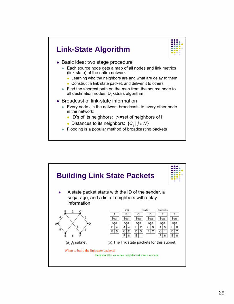
Link-State Algorithm
Basic idea: two stage procedure Each source node gets a map of all nodes and link metrics
(li k t t ) f th ti t k(link state) of the entire network Learning who the neighbors are and what are delay to them Construct a link state packet, and deliver it to others
Find the shortest path on the map from the source node to all destination nodes; Dijkstra’s algorithm
Broadcast of link-state informationEvery node i in the network broadcasts to every other node Every node i in the network broadcasts to every other node in the network: ID’s of its neighbors: Ni=set of neighbors of i Distances to its neighbors: {Cij | j Ni}
Flooding is a popular method of broadcasting packets
Building Link State Packets
A state packet starts with the ID of the sender, a seq# age and a list of neighbors with delayseq#, age, and a list of neighbors with delay information.
(a) A subnet. (b) The link state packets for this subnet.
When to build the link state packets?Periodically, or when significant event occurs.
30
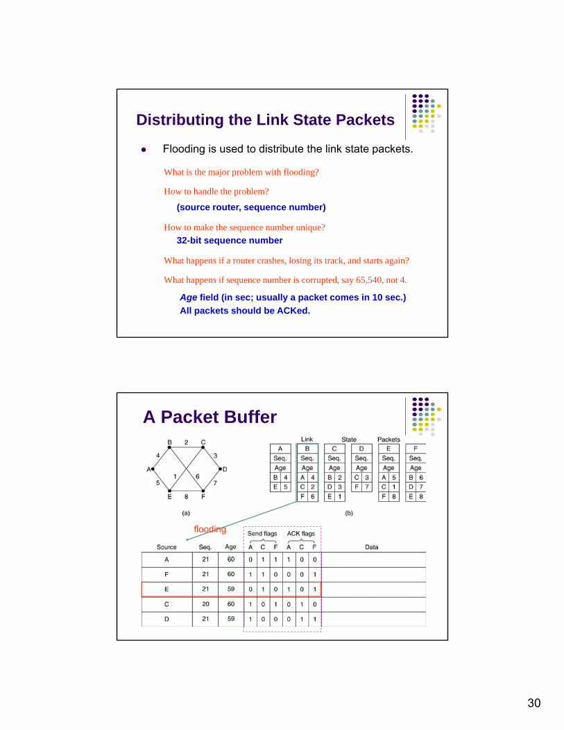
Distributing the Link State Packets
Flooding is used to distribute the link state packets.
What is the major problem with flooding?What is the major problem with flooding?
How to handle the problem?
(source router, sequence number)
How to make the sequence number unique?
32-bit sequence number
What happens if a router crashes, losing its track, and starts again?
What happens if sequence number is corrupted, say 65,540, not 4.
Age field (in sec; usually a packet comes in 10 sec.)
All packets should be ACKed.
A Packet Buffer
flooding

31
Shortest Paths in Dijkstra’s Algorithm
1
4
6
1
1
2
23
5
2 3 31
4
6
1
1
2
23
5
2 3
25
13
2
4
25
13
2
4
1
2
4
5
6
1
1
2
32
35
2 33 1
2
4
5
6
1
1
2
32
35
2 33
54 54
1
2
4
5
6
1
1
2
32
35
2
4
33 1
2
4
5
6
1
1
2
32
35
2
4
33
Execution of Dijkstra’s algorithm
16
1
25
2 3 16
1
25
2 3316
1
25
2 3 16
1
25
2 3316
1
25
2 33 16
1
25
2 3316
1
25
2 33
Iteration N D2 D3 D4 D5 D6
Initial {1} 3 2 5 1 {1 3} 3 2 4 3
2
4
5
13
23
42
4
5
13
23
4
2
4
5
13
23
4
2
4
5
13
23
4
2
4
5
13
23
4
2
4
5
13
23
42
4
5
13
23
4
1 {1,3} 3 2 4 3
2 {1,2,3} 3 2 4 7 3
3 {1,2,3,6} 3 2 4 5 3
4 {1,2,3,4,6} 3 2 4 5 3
5 {1,2,3,4,5,6} 3 2 4 5 3

32
Dijkstra’s algorithm
N: set of nodes for which shortest path already found
Initialization: (Start with source node s) N = {s}, Ds = 0, “s is distance zero from itself”
Dj=Csj for all j s, distances of directly-connected neighbors
Step A: (Find next closest node i) Find i N such that
Di = min Dj for j N
Add i to N Add i to N
If N contains all the nodes, stop
Step B: (update minimum costs) For each node j N
Dj = min (Dj, Di+Cij)
Go to Step A
Minimum distance from s to j through node i in N
Reaction to Failure
If a link fails, Router sets link distance to infinity & floods the
t k ith d t k tnetwork with an update packet All routers immediately update their link database &
recalculate their shortest paths Recovery very quick
But watch out for old update messages Add time stamp or sequence # to each update
message Check whether each received update message is new If new, add it to database and broadcast If older, send update message on arriving link

33
Why is Link State Better?
Fast, loopless convergence
Support for precise metrics and multiple Support for precise metrics, and multiple metrics if necessary (throughput, delay, cost, reliability)
Support for multiple paths to a destination algorithm can be modified to find best two paths
More flexible, e.g., source routing
What is the memory required to store the input data for a subnet with n routers – each of them has k neighbors? But not critical today!
Source Routing vs. H-by-H
Source host selects path that is to be followed by a packet Strict: sequence of nodes in path inserted into header Loose: subsequence of nodes in path specified
Intermediate switches read next-hop address and remove address Or maintained for the reverse path
Source routing allows the host to control the paths that its information traverses in the network
Potentially the means for customers to select what service providers they use
34
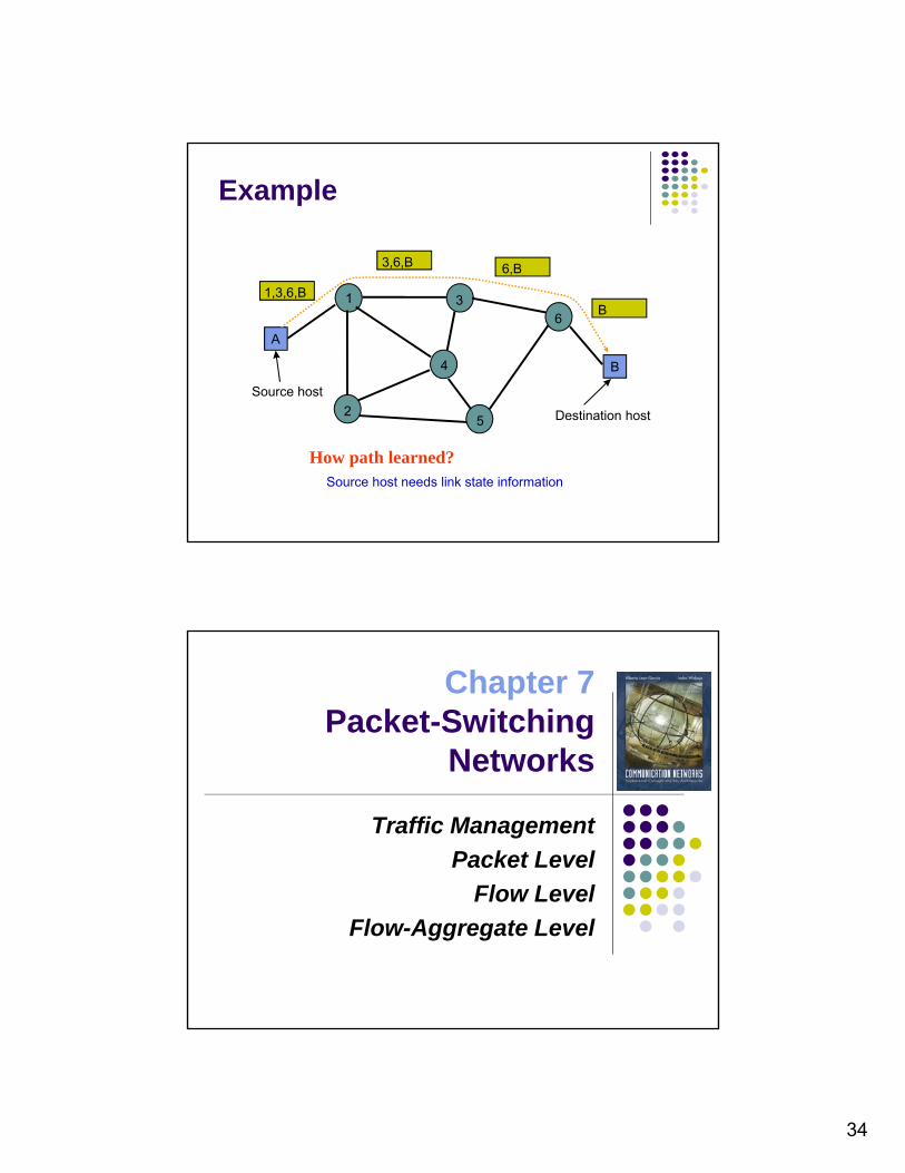
3,6,B 6,B
Example
1
2
3
4
6
A
B
Source host
1,3,6,BB
25 Destination host
How path learned?Source host needs link state information
Chapter 7Packet-Switching
NetworksNetworks
Traffic Management
Packet Level
Flow LevelFlow Level
Flow-Aggregate Level
35
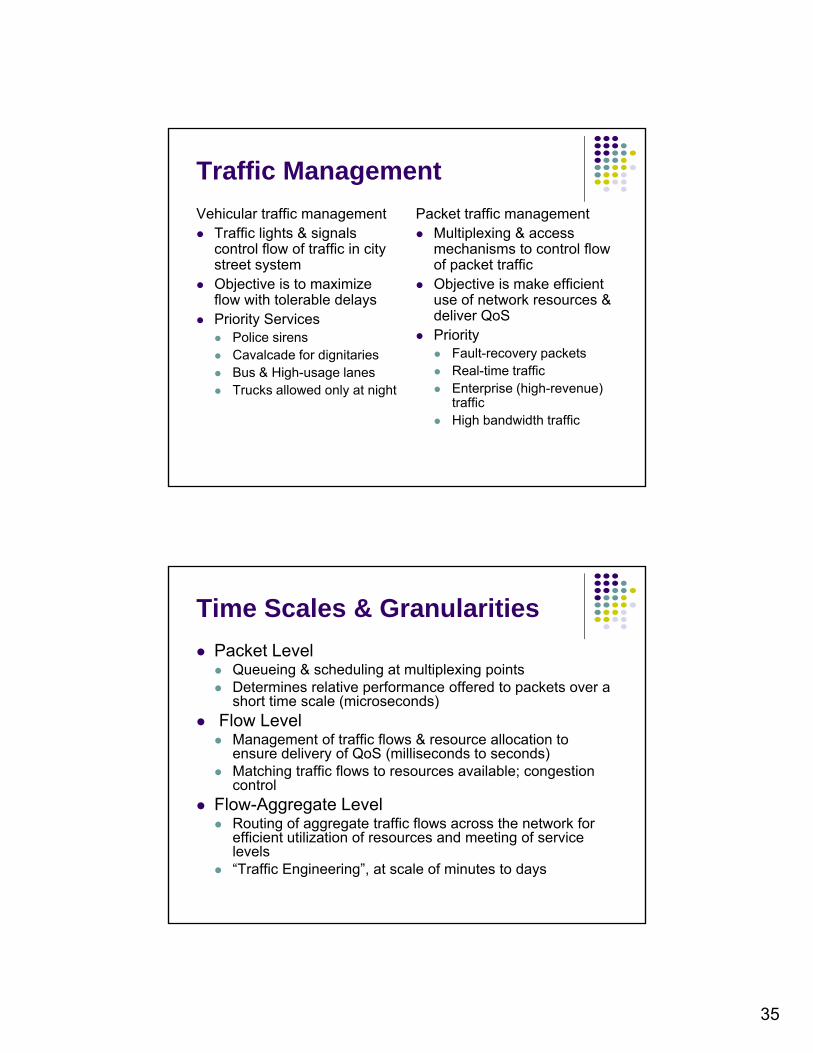
Traffic Management
Vehicular traffic management Traffic lights & signals
control flow of traffic in city
Packet traffic management Multiplexing & access
mechanisms to control flowcontrol flow of traffic in city street system
Objective is to maximize flow with tolerable delays
Priority Services Police sirens Cavalcade for dignitaries
&
mechanisms to control flow of packet traffic
Objective is make efficient use of network resources & deliver QoS
Priority Fault-recovery packets
R l ti t ffi Bus & High-usage lanes Trucks allowed only at night
Real-time traffic Enterprise (high-revenue)
traffic High bandwidth traffic
Time Scales & Granularities
Packet Level Queueing & scheduling at multiplexing points
Determines relative performance offered to packets over a Determines relative performance offered to packets over a short time scale (microseconds)
Flow Level Management of traffic flows & resource allocation to
ensure delivery of QoS (milliseconds to seconds) Matching traffic flows to resources available; congestion
control Flow Aggregate Level Flow-Aggregate Level Routing of aggregate traffic flows across the network for
efficient utilization of resources and meeting of service levels
“Traffic Engineering”, at scale of minutes to days

36
Packet buffer
End-to-End QoS
1 2 NN – 1
…
A packet traversing network encounters delay and possible loss at various multiplexing points
End-to-end performance is accumulation of per-hop performances
How to keep end-to-end delay under some upper bound? Jitter, loss?
Scheduling & QoS
End-to-End QoS & Resource Control Buffer & bandwidth control → Performance
Admission control to regulate traffic level Admission control to regulate traffic level
Scheduling Concepts fairness/isolation
priority, aggregation,
Fair Queueing & Variations WFQ, PGPS
Guaranteed Service WFQ, Rate-control
Packet Dropping aggregation, drop priorities
72
37
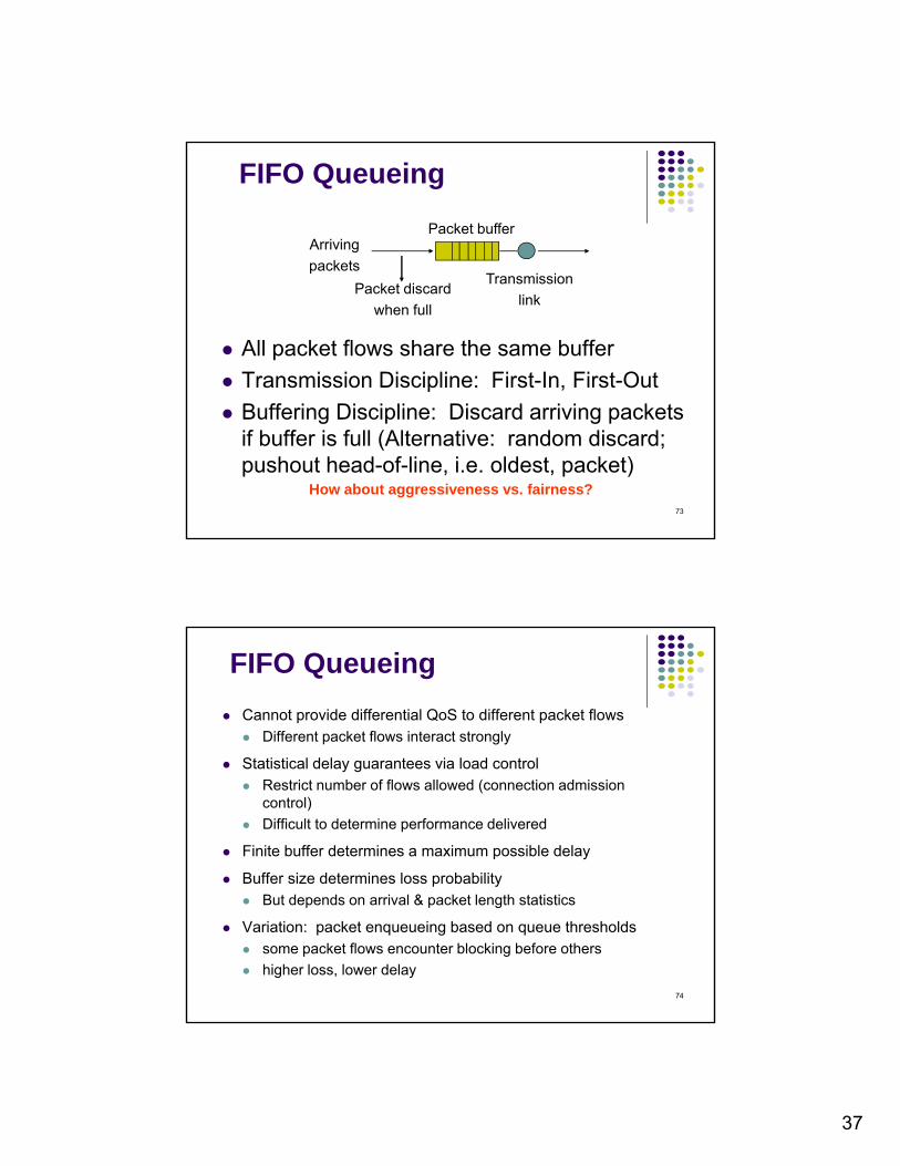
FIFO Queueing
Packet buffer
T i i
Arriving
packets
All packet flows share the same buffer
Transmission Discipline: First-In, First-Out
B ff i Di i li Di d i i k t
Transmission
linkPacket discard
when full
Buffering Discipline: Discard arriving packets if buffer is full (Alternative: random discard; pushout head-of-line, i.e. oldest, packet)
How about aggressiveness vs. fairness?73
FIFO Queueing
Cannot provide differential QoS to different packet flows Different packet flows interact strongly
St ti ti l d l t i l d t l Statistical delay guarantees via load control Restrict number of flows allowed (connection admission
control)
Difficult to determine performance delivered
Finite buffer determines a maximum possible delay
Buffer size determines loss probability But depends on arrival & packet length statistics
Variation: packet enqueueing based on queue thresholds some packet flows encounter blocking before others
higher loss, lower delay
74
38
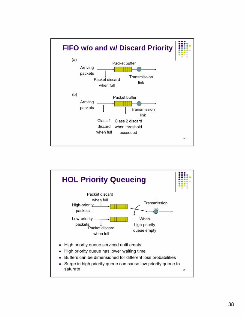
Packet bufferArriving
packets
(a)
FIFO w/o and w/ Discard Priority
Transmission
link
packets
Packet discard
when full
Packet buffer
Transmission
Arriving
packets
(b)
Transmission
linkClass 1
discard
when full
Class 2 discard
when threshold
exceeded75
HOL Priority Queueing
Transmission
Packet discard
when fullHigh-priority
linkHigh priority
packets
Low-priority
packetsPacket discard
when full
When
high-priority
queue empty
High priority queue serviced until empty
High priority queue has lower waiting time
Buffers can be dimensioned for different loss probabilities
Surge in high priority queue can cause low priority queue to saturate 76
39
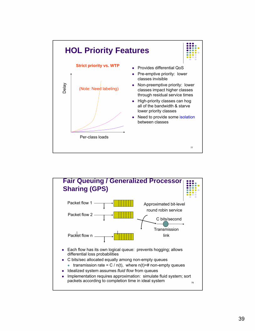
HOL Priority Features
Provides differential QoS
Pre-emptive priority: lower l i i ibl
Strict priority vs. WTP
classes invisible
Non-preemptive priority: lower classes impact higher classes through residual service times
High-priority classes can hog all of the bandwidth & starve lower priority classes
N d t id i l ti
Del
ay
(Note: Need labeling)
Need to provide some isolationbetween classes
Per-class loads
77
Fair Queuing / Generalized Processor Sharing (GPS)
Packet flow 1
Packet flow 2
Approximated bit-level
round robin service
Each flow has its own logical queue: prevents hogging; allows diff ti l l b biliti
C bits/second
Transmission
link
Packet flow 2
Packet flow n… …
differential loss probabilities C bits/sec allocated equally among non-empty queues
transmission rate = C / n(t), where n(t)=# non-empty queues Idealized system assumes fluid flow from queues Implementation requires approximation: simulate fluid system; sort
packets according to completion time in ideal system78

40
Buffer 1
at t=0
B ffer 2 1
Fluid-flow system:
both packets served
at rate ½ (overall rate :
Fair Queuing – Example 1
Buffer 2
at t=0
1
t1 2
½ (
1 unit/second)Both packets
complete service
at t = 20
Packet-by-packet system:
b ff 1 d fi t t t 1
Packet from
buffer 2 waiting
1
t1 2
buffer 1 served first at rate 1;
then buffer 2 served at rate 1.Packet from buffer 2
being servedPacket from
buffer 1 being
served
buffer 2 waiting
079
Buffer 1
at t=0
Fluid-flow system:
both packets served
at rate 1/2
2
Fair Queuing – Example 2
Buffer 2
at t=0
2
1
t3
at rate 1/2Packet from buffer 2 served at rate 1
0Service rate = reciprocal of the number of active buffers at the time.
* Within a buffer, FIFO still though!
1
t1 2
Packet-by-packet
fair queueing:
buffer 2 served at rate 1Packet from
buffer 1 served at rate 1
Packet from
buffer 2 waiting
0 380
41
Buffer 1
at t=0
Buffer 2
Fluid-flow system:
packet from buffer 1
served at rate 1/4;
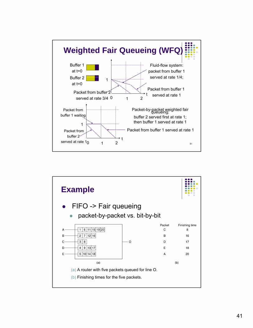
Weighted Fair Queueing (WFQ)
Buffer 2
at t=01
t1 2
served at rate 1/4;
Packet from buffer 1
served at rate 1Packet from buffer 2
served at rate 3/4 0
Packet from
b ff 1 iti
Packet-by-packet weighted fair queueing:
1
t1 2
Packet from buffer 1 served at rate 1Packet from
buffer 2
served at rate 1
buffer 1 waiting
0
buffer 2 served first at rate 1;then buffer 1 served at rate 1
81
Example
FIFO -> Fair queueingk t b k t bit b bit packet-by-packet vs. bit-by-bit
(a) A router with five packets queued for line O.
(b) Finishing times for the five packets.
42
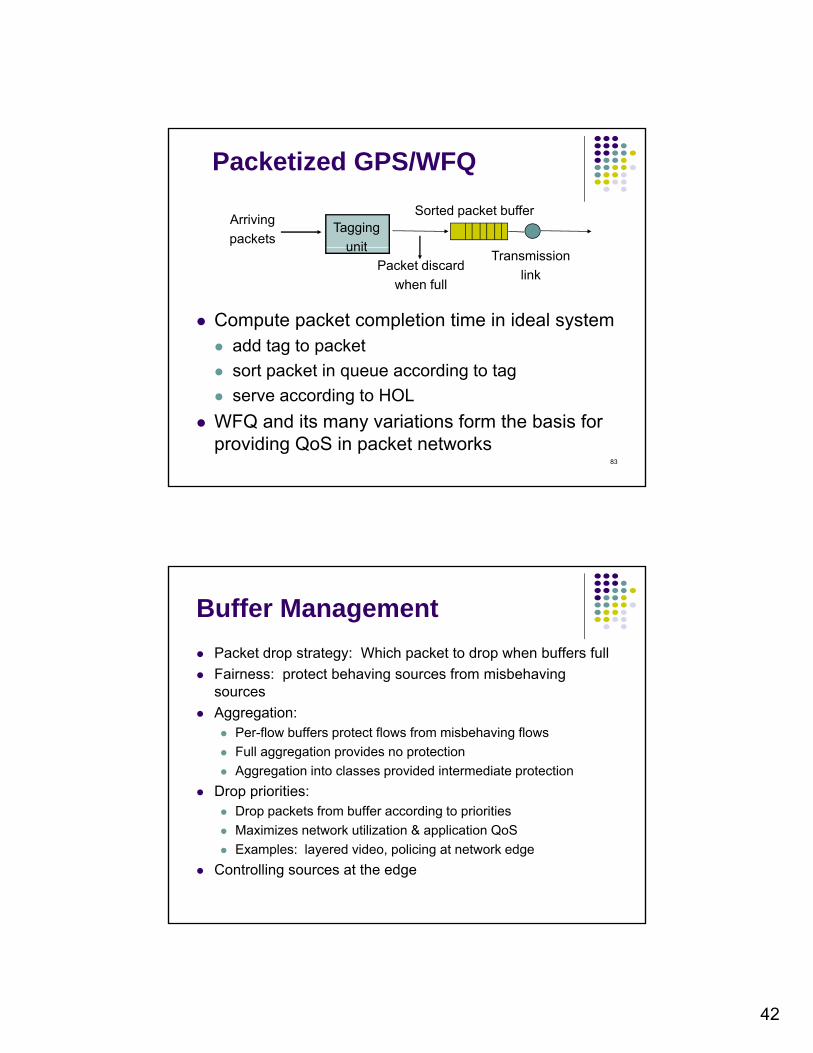
Packetized GPS/WFQ
Sorted packet bufferArriving
packetsTagging
unit
Compute packet completion time in ideal system add tag to packet
sort packet in queue according to tag
Transmission
linkPacket discard
when full
unit
sort packet in queue according to tag
serve according to HOL
WFQ and its many variations form the basis for providing QoS in packet networks
83
Buffer Management
Packet drop strategy: Which packet to drop when buffers full
Fairness: protect behaving sources from misbehaving sources
Aggregation: Per-flow buffers protect flows from misbehaving flows
Full aggregation provides no protection
Aggregation into classes provided intermediate protection
Drop priorities: Drop packets from buffer according to priorities
Maximizes network utilization & application QoS
Examples: layered video, policing at network edge
Controlling sources at the edge
43
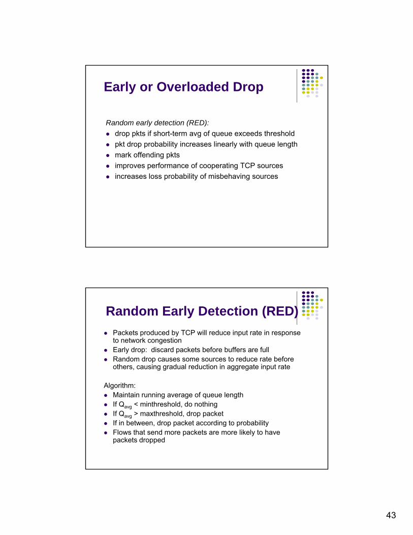
Early or Overloaded Drop
Random early detection (RED):y ( )
drop pkts if short-term avg of queue exceeds threshold
pkt drop probability increases linearly with queue length
mark offending pkts
improves performance of cooperating TCP sources
increases loss probability of misbehaving sources
Random Early Detection (RED)
Packets produced by TCP will reduce input rate in response to network congestionE l d di d k t b f b ff f ll Early drop: discard packets before buffers are full
Random drop causes some sources to reduce rate before others, causing gradual reduction in aggregate input rate
Algorithm: Maintain running average of queue length If Qavg < minthreshold, do nothingg
If Qavg > maxthreshold, drop packet If in between, drop packet according to probability Flows that send more packets are more likely to have
packets dropped
44
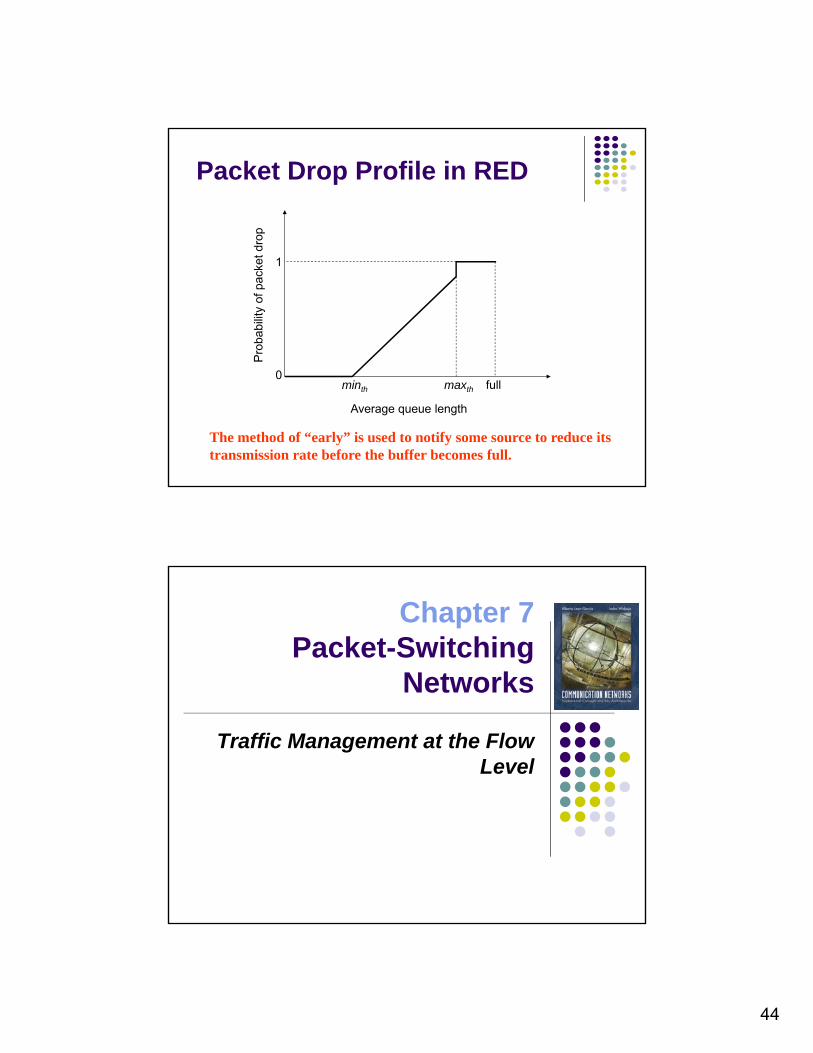
drop
Packet Drop Profile in RED
Pro
babi
lity
of p
acke
t d
1
Average queue length
0minth maxth full
The method of “early” is used to notify some source to reduce its transmission rate before the buffer becomes full.
Chapter 7Packet-Switching
NetworksNetworks
Traffic Management at the Flow Level
45
63
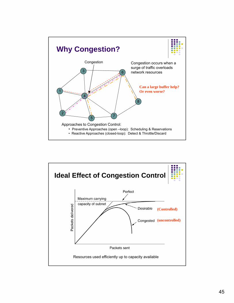
Congestion Congestion occurs when a surge of traffic overloads
t k
Why Congestion?
4
8
63
1
network resources
Can a large buffer help? Or even worse?
25
7
Approaches to Congestion Control:• Preventive Approaches (open –loop): Scheduling & Reservations• Reactive Approaches (closed-loop): Detect & Throttle/Discard
Ideal Effect of Congestion Control
(Controlled)
(uncontrolled)
Resources used efficiently up to capacity available

46
Open-Loop Control
Network performance is guaranteed to all traffic flows that have been admitted into thetraffic flows that have been admitted into the network
Initially for connection-oriented networks
Key Mechanisms Admission Control
Policing
Traffic Shaping
Traffic Scheduling
Peak rate
Admission Control
Flows negotiate contract with network
Specify requirements:
Bits
/sec
ond
Peak rate
Average rate
Specify requirements: Peak, Avg., Min Bit rate Maximum burst size Delay, Loss requirement
Network computes resources needed “Effective” bandwidth
Time
Typical bit rate demanded by a variable bit rate information source
If flow accepted, network allocates resources to ensure QoS delivered as long as source conforms to contract
47
Policing
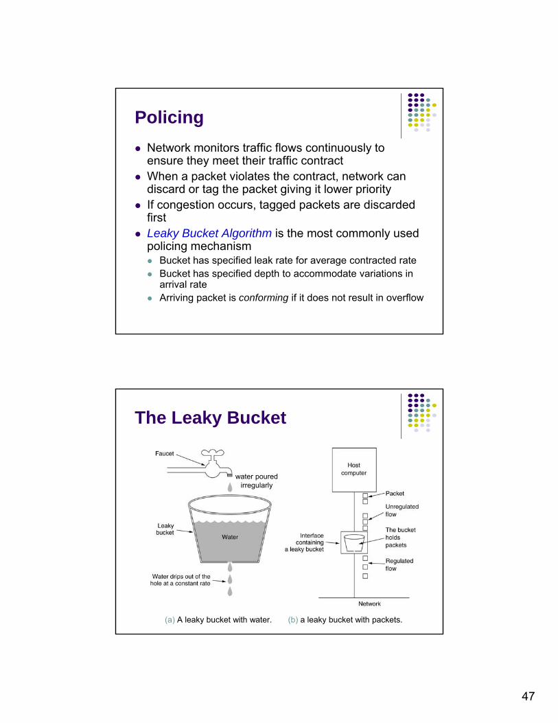
Network monitors traffic flows continuously to ensure they meet their traffic contract
When a packet violates the contract, network can discard or tag the packet giving it lower priority
If congestion occurs, tagged packets are discarded first
Leaky Bucket Algorithm is the most commonly used policing mechanismp g Bucket has specified leak rate for average contracted rate Bucket has specified depth to accommodate variations in
arrival rate Arriving packet is conforming if it does not result in overflow
The Leaky Bucket
water pouredirregularly
(a) A leaky bucket with water. (b) a leaky bucket with packets.

48
Data comes to a router in 1 MB bursts, that is, an
The Leaky Bucket Example
, ,input runs at 25 MB/s (burst rate) for 40 msec. The router is able to support 2 MB/s output (leaky) rate. The router uses a leaky bucket for traffic shaping.
(1) How large the bucket should be so there is no data loss (assuming fluid system)?data loss (assuming fluid system)?
(2) Now, if the leaky bucket size is 1MB, how long the maximum burst interval can be?
The Leaky Bucket Example
° Example: data comes to a router in 1 MB bursts, that is, an input runs at 25 MB/s for 40 msec The router is able to supportinput runs at 25 MB/s for 40 msec. The router is able to support 2 MB/s outgoing (leaky) rate. The leaky bucket size is 1MB.
(a) Input to a leaky bucket. (b) Output from a leaky bucket.

49
Arrival of a packet at time ta
X’ = X - (ta - LCT)
Depletion rate: 1 packet per unit time
Leaky Bucket Algorithm
X’ < 0?
X’ > L?
X’ = 0
Nonconforming
Yes
No
Yes
L+I = Bucket Depth
I = increment per arrival, nominal interarrival time
Interarrival timeCurrent bucket
content
empty
Non-empty
X’ > L?
X = X’ + ILCT = ta
conforming packet
Nonconformingpacket
X = value of the leaky bucket counterX’ = auxiliary variable
LCT = last conformance time
Noarriving packet
would cause
overflow
conforming packet
Packetarrival
NonconformingI = 4 L = 6
Leaky Bucket Example
I
L+I
Bucketcontent
Time
Per-packet
Time* * * * * * * **
Non-conforming packets not allowed into bucket & hence not included in calculations maximum burst size (MBS = 3 packets)
not fluid system
50
Incoming traffic Shaped trafficSize N
Server
Leaky Bucket Traffic Shaper
Packet
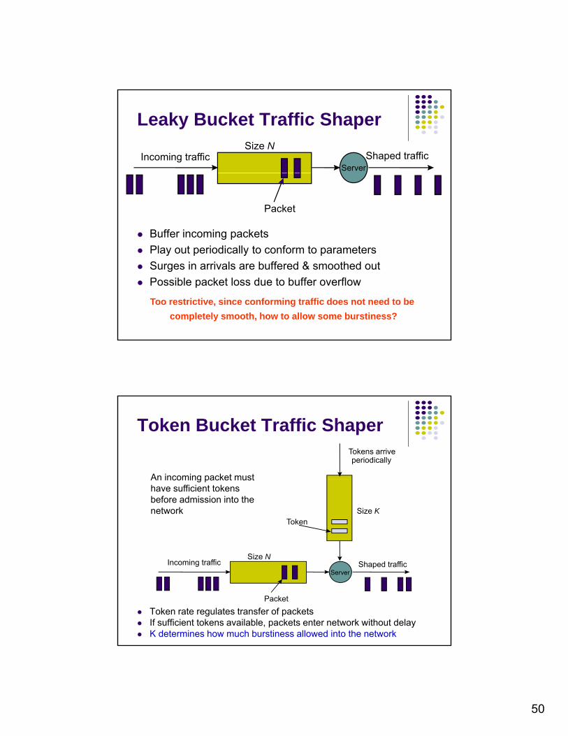
Buffer incoming packets
Play out periodically to conform to parameters
Surges in arrivals are buffered & smoothed out
Possible packet loss due to buffer overflow
Too restrictive, since conforming traffic does not need to be
completely smooth, how to allow some burstiness?
Tokens arriveperiodically
Token Bucket Traffic Shaper
An incoming packet must
Incoming traffic Sh d t ffiSize N
Size KToken
An incoming packet must have sufficient tokens before admission into the network
Incoming traffic Shaped trafficServer
Packet
Token rate regulates transfer of packets If sufficient tokens available, packets enter network without delay K determines how much burstiness allowed into the network
51
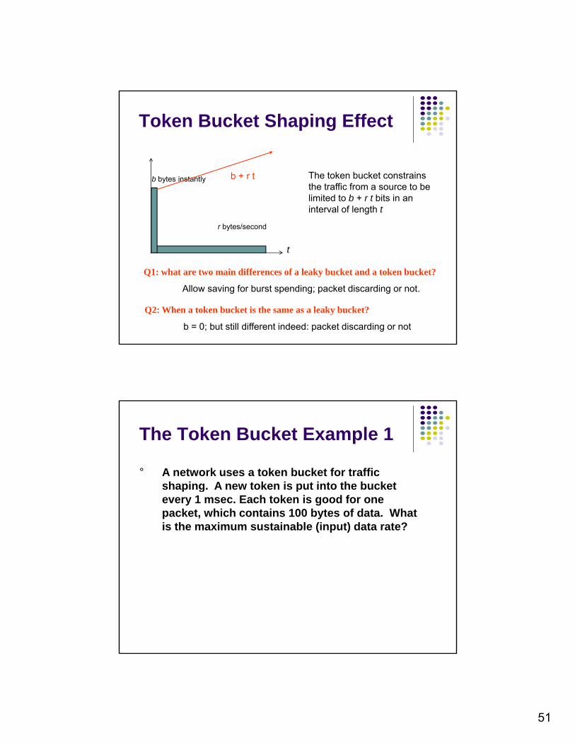
The token bucket constrains
Token Bucket Shaping Effect
b + r t The token bucket constrains the traffic from a source to be limited to b + r t bits in an interval of length t
b bytes instantly
t
r bytes/second
b + r t
Q2: When a token bucket is the same as a leaky bucket?
Q1: what are two main differences of a leaky bucket and a token bucket?
Allow saving for burst spending; packet discarding or not.
b = 0; but still different indeed: packet discarding or not
The Token Bucket Example 1
° A network uses a token bucket for traffic shaping A new token is put into the bucketshaping. A new token is put into the bucket every 1 msec. Each token is good for one packet, which contains 100 bytes of data. What is the maximum sustainable (input) data rate?
52
° Given: the token bucket capacity C, the token arrival rate
The Token Bucket Example 2
p, and the maximum output rate M, calculate the maximum burst interval S
C + pS = MS
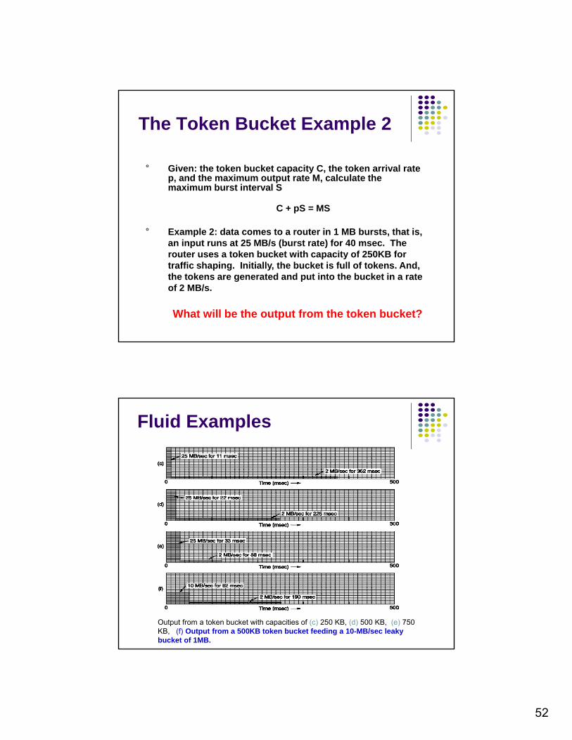
° Example 2: data comes to a router in 1 MB bursts, that is, an input runs at 25 MB/s (burst rate) for 40 msec. The router uses a token bucket with capacity of 250KB for p ytraffic shaping. Initially, the bucket is full of tokens. And, the tokens are generated and put into the bucket in a rate of 2 MB/s.
What will be the output from the token bucket?
Fluid Examples
Output from a token bucket with capacities of (c) 250 KB, (d) 500 KB, (e) 750 KB, (f) Output from a 500KB token bucket feeding a 10-MB/sec leaky bucket of 1MB.
53
RoutingAgent
ReservationAgent
Mgmt.Agent
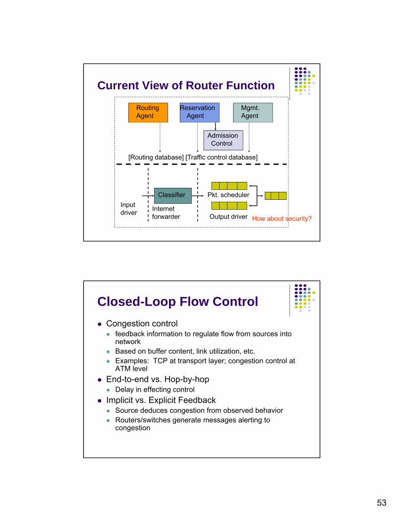
Current View of Router Function
AdmissionControl
[Routing database] [Traffic control database]
Classifier
Inputdriver
Internetforwarder
Pkt. scheduler
Output driver How about security?
Closed-Loop Flow Control
Congestion control feedback information to regulate flow from sources into
t knetwork Based on buffer content, link utilization, etc. Examples: TCP at transport layer; congestion control at
ATM level
End-to-end vs. Hop-by-hop Delay in effecting control
Implicit vs Explicit Feedback Implicit vs. Explicit Feedback Source deduces congestion from observed behavior Routers/switches generate messages alerting to
congestion
54
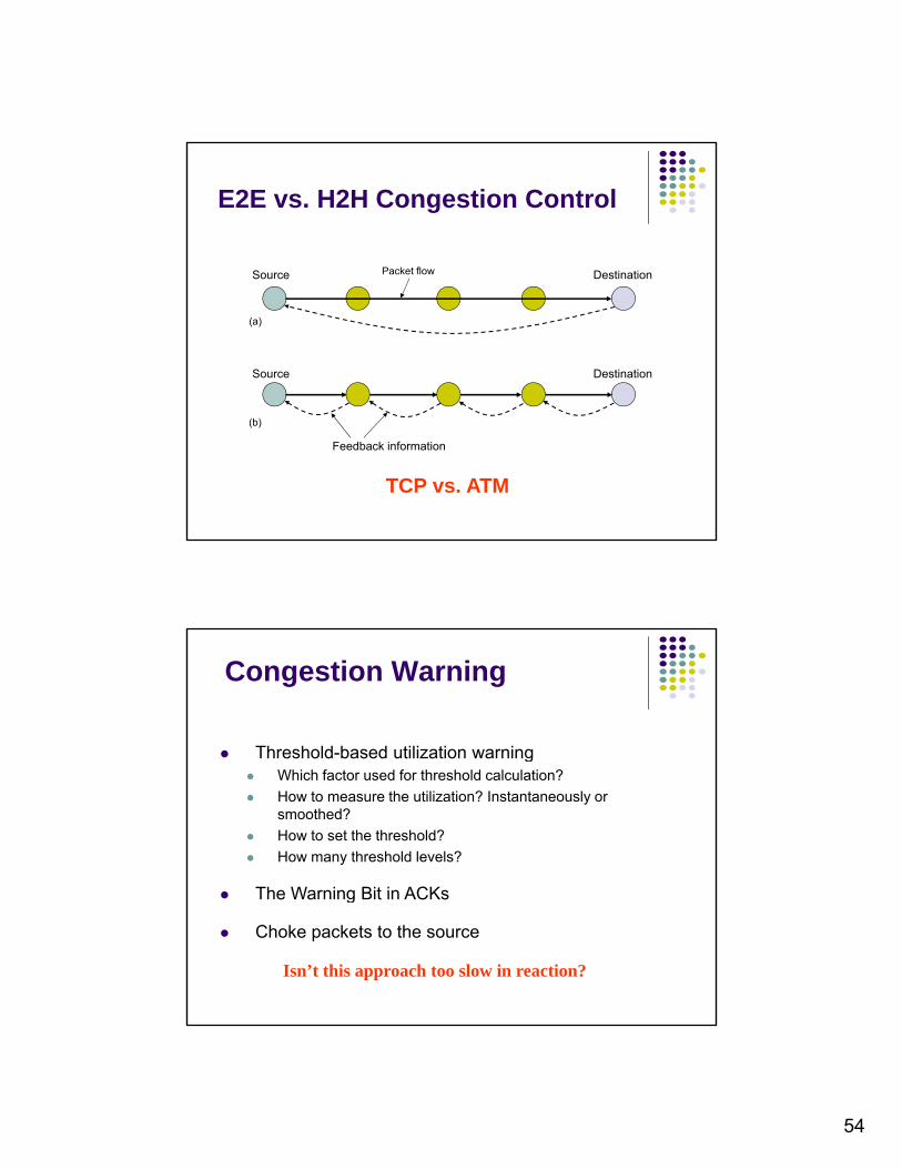
Source DestinationPacket flow
E2E vs. H2H Congestion Control
Source Destination
Source Destination
(a)
Feedback information
(b)
TCP vs. ATM
Congestion Warning
Threshold-based utilization warningg Which factor used for threshold calculation?
How to measure the utilization? Instantaneously or smoothed?
How to set the threshold?
How many threshold levels?
The Warning Bit in ACKs The Warning Bit in ACKs
Choke packets to the source
Isn’t this approach too slow in reaction?
55
Traffic Engineering
Management exerted at flow aggregate level
Distribution of flows in network to achieve efficientDistribution of flows in network to achieve efficient utilization of resources (bandwidth)
Shortest path algorithm to route a given flow not enough Does not take into account requirements of a flow, e.g.
bandwidth requirement
Does not take account interplay between different flows Does not take account interplay between different flows
Must take into account aggregate demand from all flows
63 63
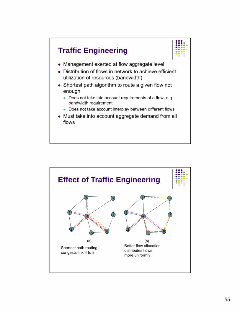
Effect of Traffic Engineering
4
2
1
5 8
7 4
2
1
5 8
7
(a) (b)
Shortest path routing congests link 4 to 8
Better flow allocation distributes flows more uniformly
Related Documents