Chapter 7 First-order Differential Equations 7 First-order Differential...The solution of the differential equation in Equation (a) is available in Equation (7.4), or in the form:

Chapter 7

Application of First-order Differential Equations in Engineering Analysis

(Chapter 7 First order DEs)© Tai-Ran Hsu

* Based on the book of “Applied Engineering Analysis”, by Tai-Ran Hsu, published byJohn Wiley & Sons, 2018

Applied Engineering Analysis- slides for class teaching*

Chapter Learning Objectives

● Learn to solve typical first order ordinary differential equations of both homogeneous and non‐homogeneous types with or without specified conditions.

● Learn the definitions of essential physical quantities in fluid mechanics analyses.

● Learn the Bernoulli’s equation relating the driving pressure and the velocities of fluids in motion.

● Learn to use the Bernoulli’s equation to derive differential equations describing the flow of non‐compressible fluids in large tanks and funnels of given geometry.

● Learn to find time required to drain liquids from containers of given geometry and dimensions.

● Learn the Fourier law of heat conduction in solids and Newton’s cooling law for convective heat transfer in fluids.

● Learn how to derive differential equations to predict required times to heat or cool small solids by surrounding fluids.

● Learn to derive differential equations describing the motion of rigid bodies under the influence of gravitation.

7.1 Introduction on Differential Equations

Types of Differential equations:

We have learned in Chapter 2 that differential equations are the equations that involve “derivatives.”

They are used extensively in mathematical modeling of engineering and physical problems.

There are generally two types of differential equations used in engineering analysis. These are:

1. Ordinary differential equations (ODE): Equations with functions that involve only one variable and with different orders of “ordinary” derivatives , and

2. Partial differential equations (PDE): Equations with functions that involve more than one variable and with different orders of “partial” derivatives.

How differential equations are derived?

They are derived from the three fundamental laws of physics of which most engineering analyses involve. These laws are:

(1) The law of conservation of mass,(2) The law of conservation of energy, and (3) The law of conservation of momentum.

7.1 Introduction on Differential Equations – Cont’d

Differential equations for mechanical engineering:

For mechanical engineering analyses, frequently used laws of physics include the following:

● The Newton’s laws for statics, dynamics and kinematics of solids.● The Fourier’s law for heat conduction in solids.● The Newton cooling law for convective heat transfer in fluids.● The Bernoulli’s principle for fluids in motion.● Fick’s law for  diffusion of substances with different densities● Hooke’s law for deformable solids

7.2 Review of Solution Methods forFirst Order Differential Equations

In “real-world,” there are many physical quantities that can be represented by functionsinvolving only one of the four independent variables e.g., (x, y, z, t), in which variables (x,y,z)For space and variable t for time.

First order differential equations are the equations that involve highest order derivatives of order one . They are often called “the 1st order differential equations

Examples of first order differential equations:

Function σ(x)= the stress in a uni-axial stretched metal rod with tapered cross section (Fig. a), or Function v(x)=the velocity of fluid flowing in a straight channel with varying cross-section (Fig. b):

x

Figure a xv(x)

σ(x)

Figure b

Mathematical modeling using differential equations involving these functions are classified asFirst Order Differential Equations

7.2.1 Solution Methods for Separable First Order ODEs

)()()( xgdx

xduuh

Typical form of the first order differential equations:

(7.1)

in which h(u) and g(x) are given functions.By re‐arranging  the terms in Equation (7.1) the following form with the left‐hand‐side (LHS) involves function of u (or constants) only, and the right‐hand‐side (RHS) consists of function of the variable g(x) (or constants) only :

h(u) du = g(x) dx

Solution u(x) of Equation (7.1) may be obtained by integrating both sides of the above equality and resulting in:

cdxxgduuh )()( (7.2)

where c is the integration constant to be determined by given specified condition for the problem.Example 7.1 Solve the following first order ordinary differential equation: 4)( 2 u

dxxdux

By re‐arranging the terms in the DE into the separated form with the LHS involving the function u(x) and the RHS with the variable x:

Solution:

xdx

xudu

2)(4

followed by integrating both sides to get: cxnuun

22

41 with c=integration constant

The solution u in the above expression may be re‐written in the following form:

1'1'2)( 4

4

xcxcxu with c’ being another arbitrary constant to be 

determined by specified condition

Typical form of the equation:

0)()()( xuxp

dxxdu

The solution u(x) in the above equation is:

xFKxu

where K = constant to be determined by given condition, and the function F(x) has the form:

dxxp

exF)(

)(in which the function p(x) is given in the differential equation in Equation (7.3)

7.2.2 Solution of linear, homogeneous equations

(7.3)

(7.4)

(7.5)

Example 7.2

7.2.2 Solution of linear, homogeneous equations – Cont’d

Solve the following first order ordinary differential equation: xxu

dxxdu sin (a)

We will first re‐arrange the terms in Equation (a) in the following way:Solution:

0)(sin)( xux

dxxdu

By comparison,  we have: p(x) = ‐sin x, which leads to the integral: xdxxp cosand hence have: xdxxp

eexF cos)()( from Equation (7.5)

The solution of the differential equation in Equation (a) is available in Equation (7.4), or in the form:  

xc

KexF

exu cos

)()(

where K is an arbitrary constant to be determined by an appropriate prescribed condition.

7.2.3 Solution of linear Non-homogeneous equations:

Typical differential equation:

)()()()( xgxuxpdx

xdu (7.6)

The appearance of function g(x) in Equation (7.6) makes the DE non-homogeneous

The solution of ODE in Equation (7.6) is similar to the solution of homogeneous equation in a little more complex form than that for the homogeneous equation in (7.3):

)(

)()()(

1)(xF

KdxxgxFxF

xu (7.7)

dxxp

exF)(

)(

where function F(x) can be obtained from Equation (7.5) as:

(7.5)

dxxp

exF)(

)( is called the “integration factor,”where the integral in Equation (7.5)

and K is the integration constant.

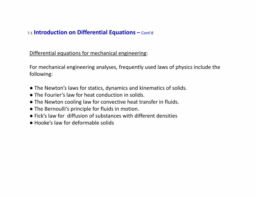
Example 7.3Solve the following first order non‐homogeneous differential equation:

xxudx

xdux 5)(2)(2

Solution:By re‐arranging the terms, we get:

xxu

xdxxdu 5)(2)(

2 (a)

xxgand

xxp 5)(2)( 2

By comparison of Equations (a) and (7.6), we get:

The integration factor in Equation (7.5) is  xdx

xdxxpeeexF

22)( 2)(

The solution of Equation (a), u(x) is obtained by substituting the above integration factor into Equation (7.7) and resulted in:

xx

xx

x

x

Kedxexee

Kdxx

ee

xFKdxxgxF

xFxu

221

22

2

2

551)(

)()()(

1)(

The integration constant K in the above solution of this ODE can be determined by specified conditions, as will be demonstrated in the next example ‐ Example 7.4.

Example 7.4Solve the following differential equation:

2)(2)( xu

dxxdu

with a given condition: u(0) = 2   

Solution:

By comparison of Equation (a) with the typical form in Equation (7.6), we will have: p(x) = 2 and g(x) = 2.

(a)(b)

Thus, from Equation (7.5), we get:  xdxdxxpeeexF 22)(

)(

Following Equation (7.7), we have the solution of Equation (a) as

xxx

x eK

eKdxe

exFKdxxgxF

xFxu 22

22 121

)()()(

)(1)( (c)

The integration constant K may be determined by using the specified condition in Equation (b) with u(x) = 2 at x = 0. Thus by substituting this condition into Equation (c), we will get the relationship: 21

02

xxe

K from which we may obtain K = 1

Consequently, we have the complete solution of u(x) in Equation (a) to be:

xx e

exu 2

2 111)(

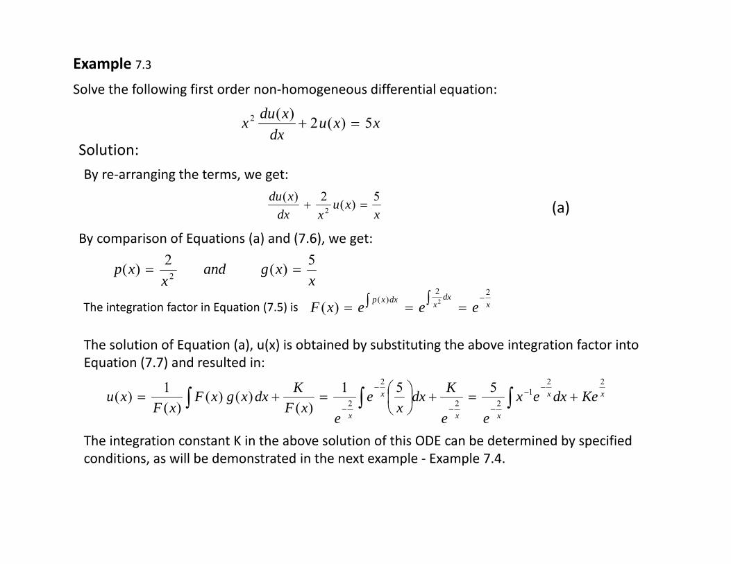
7.3 Application of First Order Differential Equation to  Fluid Mechanics Analysis

Fundamental Principles of Fluid Mechanics Analysis:

Fluids

Compressible(Gases)

Non-compressible(Liquids)

- A substance with mass but no shape

Moving of a fluid requires:

● A conduit, e.g., tubes, pipes, channels, etc.● Driving pressure, or by gravitation, i.e., difference in “head”● Fluid flows with a velocity v from higher pressure (or elevation) to

lower pressure (or elevation)● Fluid flows from higher elevation to low elevation

tvAQ

sec)/(kgvAt

QQ

sec)/( 3mAvQV

)( 3mtvAtVV

The total mass flow,

Total mass flow rate,

Total volumetric flow rate,

Total volumetric flow,

Fluid velocity, vCross-sectional

Area, A

Fluid flow

Higher pressure (or elevation)

7.3.1 Common Terminologies in Fluid Mechanics Analysis

(7.8a)

(7.8b)

(7.8c)

(7.8d)

in which ρ = mass density of fluid (g/m3), A = cross-sectional area (m2), v = velocity (m/s), and ∆t = duration of fluid flow (s).

The units associated with the above quantities are (kg) for kilograms, (m) for meters and (sec) for seconds.

● In case the velocity varies with time, i.e., v = v(t):Then the change of volumetric flow becomes: ∆V = A v(t) ∆t, with ∆t = time duration for the fluid flow

(7.9)

Lower pressure (or elevation)

kg

7.3.2 The Bernoulli Equation(It is the mathematical expression of the law of physics that relates the driving pressure

and velocity in a moving non-compressible fluid)

(State 1) (State 2)

Velocity, v1

Velocity, v 2

Pressure, p1

Pressure, p2

Elevation, y1

Elevation, y2

Reference plane

Using the Law of conservation of energy, or the First Law of Thermodynamics, for theenergies of the fluid at State 1 and State 2, we can derive the following expression relating driving pressure (p) and the resultant velocity of the flow (v):

22

22

11

21

22y

gp

gv

yg

pg

v

The Bernoulli Equation:

Application of Bernoulli equation in liquid (water) flow in a LARGE reservoir:

Ele

vatio

n, y

1

y2

v2, p2

v1, p1

Fluid level

Hea

d, h

Reference plane

State 1

State 2

LargeReservoir W

ater

tank

Tap exit

From the Bernoullis’s equation, we have:

02 21

2122

21

yygpp

gvv

(7.10)

Tap exit

If the difference of elevations between State 1 and 2 is not too large, we can have: p1 ≈ p2

Also, because it is a LARGE reservoir (or tank), we realize that v1 << v2, or v1≈ 0

Equation (7.10) can thus be reduced to the form: 21

22 00

2yyhwithh

gv

from which, we may express the exit velocity of the liquid at the tap, i.e. v2 to be:

ghv 22 (7.11)

We assume the friction between the moving fluids and their containing wall is negligiblein all cases.

A1

A1

A2

A2

v1v2

The rate of volumetric flow follows the rule:

q = A1v1 = A2v2 m3/s

7.3.3 The Continuity Equation

This equation is derived from the law of conservation of mass. By referring to the situation depicted in figure below, the non-compressible fluids (for most liquids) flow from a section of a pipeline with larger cross-sectional area A1 to a section with smaller cross-sectional area A2.

(7.12)

D

d

X-secti

onal

area,

A

ho hoh(t) H2O

Initial water level = ho

Water level at time, t = h(t)

Velocity, v(t)

7.4 Liquid Flow in Reservoirs, Tanks and Funnels

Tap Exit

The physical condition for math modeling: The law of conservation of mass requires:

The total volume of water leaving the tank at the exit during ∆t: (∆Vexit) =The total volume of water supplied by the tank during ∆t: (∆Vtank)

We have from Equation (7.8d): ∆V = A v(t) ∆t, in which v(t) is the velocity of moving fluid

Thus, the volume of water leaving the tap exit is:

tthgdttvAVexit

)(2

4)(

2 (a)

where )(2)( thgtv is the instantaneous velocity of the water at the exit following the

7.4.1 Derivation of differential equations and drainage of a large tank or reservoir:

expression in Equation (7.11), and h(t) is the instantaneous water level in the reservoir.

Next, we need to formulate the water supplied by the tank, ∆Vtank:

ho

h(t)

∆h(t)

Velocity, v(t)

H2O

D

d

The given initial water level in the tank is ho

The water level keeps dropping after thetap exit is opened, and the reduction ofwater level is CONTINUOUS with time t

Let the water level at time t be h(t)

We let ∆h(t) = amount of drop of water level during time increment ∆t

Then, the volume of water LOSS in the circular tank is: )(4

2

tan thDV k

(Caution: a “-” sign is given to ∆Vtank ,b/c of the LOSS of water volume with increasing time ∆t

The total volume of water leaving the tank during ∆t (∆Vexit) in Equation (a) =The total volume of water supplied by the tank during ∆t (∆Vtank) in Equation (b):

(b)

)(4

)(24

22

thDtthgd

(c)

Thus, by equating Equation (a) Equation (b), we get:

gDdth

tth 2)()(

2

22/1

or by re-arranging the above:

(d)

=

If the process of draining is indeed CONTINUOUS, i.e., ∆t → 0, we will have Equation (d) expressed in the “differential” rather than “difference” form as follows:

)(2)(2

2

thDdg

dttdh

(7.13)

Equation (7.13) is the 1st order differential equation for the CONTINUOUS draining of a water tank.

with an initial condition of h(0) = ho

The solution of Equation (7.13) can be obtained by separating the solution h(t) and the variable t by re-arranging the terms in the following way:

dtDdg

thtdh

2

2

2)()(

Upon integrating on both sides:

cdt

Ddgdhh 2

22/1 2 where c = integration constant

from which, we obtain the solution of Equation (7.13) to be: ctDdgh

2

22/1 22

The constant ohc 2 is determined from the initial condition in Equation (f).

(f)

The complete solution of Equation (7.13) with the initial condition in Equation (f) is thus:2

2

2

2)(

oht

Ddgth (7.14)

7.4.2 Solution of differential equations

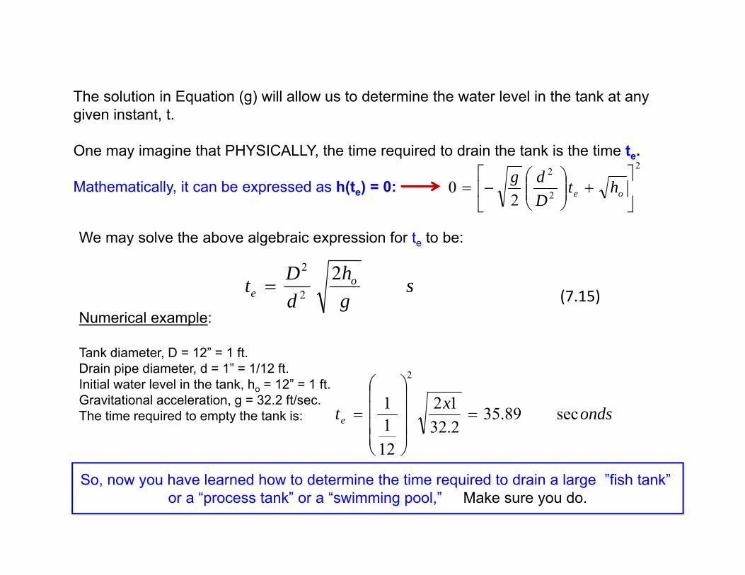
The solution in Equation (g) will allow us to determine the water level in the tank at any given instant, t.

One may imagine that PHYSICALLY, the time required to drain the tank is the time te.

Mathematically, it can be expressed as h(te) = 0:2

2

2

20

oe ht

Ddg

We may solve the above algebraic expression for te to be:

sgh

dDt o

e2

2

2

Numerical example:

Tank diameter, D = 12” = 1 ft.Drain pipe diameter, d = 1” = 1/12 ft.Initial water level in the tank, ho = 12” = 1 ft.Gravitational acceleration, g = 32.2 ft/sec.The time required to empty the tank is: ondsxte sec89.35

2.3212

1211

2

So, now you have learned how to determine the time required to drain a large ”fish tank” or a “process tank” or a “swimming pool,” Make sure you do.

(7.15)

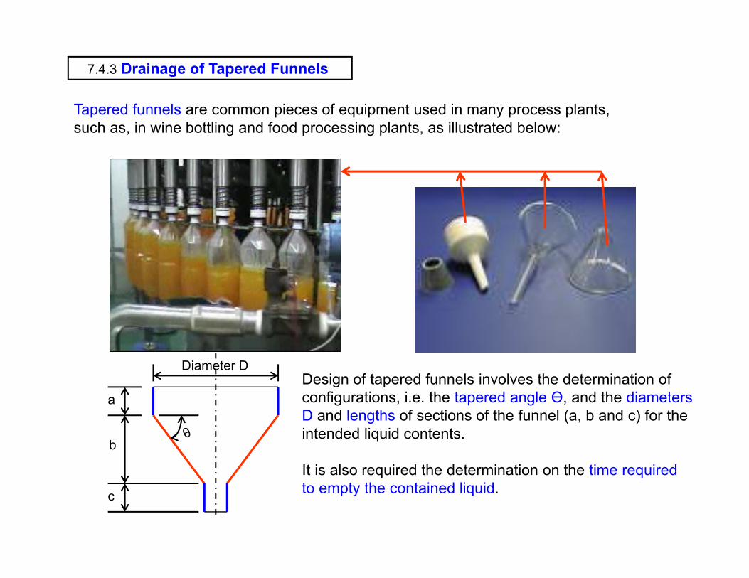
7.4.3 Drainage of Tapered Funnels

Tapered funnels are common pieces of equipment used in many process plants, such as, in wine bottling and food processing plants, as illustrated below:

Design of tapered funnels involves the determination of configurations, i.e. the tapered angle ϴ, and the diametersD and lengths of sections of the funnel (a, b and c) for the intended liquid contents.

It is also required the determination on the time required to empty the contained liquid.

a

b

c

Diameter D

Formulations on Water or Liquid Level in Tapered Funnels

The “real” funnel has an outline of frustum conewith smaller circular opening in the bottom end “A” allowing the contained liquid to leave the funnel.In the subsequent analysis, we assume the funnelhas an outline shape of “right cone” with its tip at “O” Instead.

The total volume of liquid leaving the funnel during ∆t (∆Vexit) =The total volume of liquid supplied by the funnel during ∆t (∆Vfunnel)

We assume the initial water level in the funnel = H

Once the funnel exit is open, and the liquid begins to flow.  The liquidlevel in the funnel at given time t is represented by the function y(t).

Initi

al w

ater

leve

l H

Small (negligible)Funnel opening

diameter d

y(t)

Funnel exit

We will use the same principle in Section 7.4 .1 to formulate the expression for y(t) for the straight tank:

The physical solution we are seeking is the water level at ANY given time t, y(t) after the water is let to flow from the exit of the funnel at t = 0+.

o

A

Initi

al w

ater

leve

l H

SmallFunnel openingdiameter d

y(t)

Funnel exitvelocity ve

Determine the Instantaneous Water Level in a Tapered Funnel, y(t):

Drop waterlevel

-∆yr(y)

o

A

The total volume of water leaving the tank during ∆t: (∆Vexit) = (Aexit) (ve) (∆t)

But from Equation (7.11), we have the exit velocity veto be: tygve 2which leads to the exit volume of water to be:

ttygdVexit 24

2(7.16)

The total volume of water supplied by the tank during ∆t:∆Vfunnel = volume of the cross-hatched “water disk” in the diagram

∆Vfunnel = - [π (r(y)2] (∆y)A “‐ve” sign to indicate decreasing ∆Vfunnel with increasing  y(t)

From the diagram in the left, we have: tantyyr

(7.17)

(7.18)

Hence by equating (7.16) and (7.17) with r(y) given in (7.18), we have:

ytyttygd

2

22

tan2

4(7.19)

For a CONTINUOUS variation of y(t), we have ∆t→0, we will have the differential equation for y(t) as: gd

dttdyty 2

4tan

2

2

23

(7.20)

Example 7.6

Determine the time required to drain a tapered funnel with a taper angle 45o as shown in figure below. The funnel contains water with an initial level H = 150 mm. 

Opening dia, d = 6 mm

Initi

al le

vel,

H =

150

mm

dy

y(t)r(y)

small

45o

vexit

Volume lossin ∆t = -∆V

Solution:According to Equation (7.12), the rate of volumetric flow of water leaving the funnel, qe (or  

V

in ft3/s) is qe = Ae vexit , in which the cross‐sectional area of the funnel at the exit: 4

2dAe

But as we have, from the Bernoulli equation and Equation (7.11), the exit velocity at the bottom of the funnel to be:  )(2 tygvexit

We thus have the total volumetric flow of water continuously leaving the funnel during time interval Δt (or dt in a continuous flow process) to be:

ttygdtqV ee )(24

2 (a)

The water supply in this case can be related to the drop of water level at the “upstream” in the funnel as expressed by the following equation:

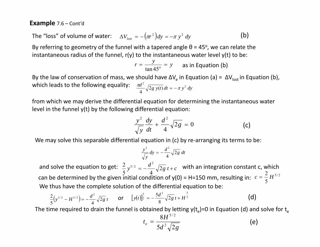
Example 7.6 – Cont’d

The “loss” of volume of water: dyydyrVlost22 (b)

By referring to geometry of the funnel with a tapered angle θ = 45o, we can relate the instantaneous radius of the funnel, r(y) to the instantaneous water level y(t) to be:

yyr o 45tan

By the law of conservation of mass, we should have ΔVe in Equation (a) =  ΔVlost in Equation (b), which leads to the following equality: dyydttygd 2

2

)(24

from which we may derive the differential equation for determining the instantaneous water level in the funnel y(t) by the following differential equation:

024

22

gddtdy

yy

(c)

dtgddyy

y 24

22

We may solve this separable differential equation in (c) by re‐arranging its terms to be:

and solve the equation to get: ctgdy 245

2 22/5 with an integration constant c, which

can be determined by the given initial condition of y(0) = H=150 mm, resulting in:   2/5

52 Hc

We thus have the complete solution of the differential equation to be:

tgdHy 245

2 22/52/5 2

52

25

28

5 Htgdty or (d)

The time required to drain the funnel is obtained by letting y(te)=0 in Equation (d) and solve for te

gdHte 25

82

2/5

(e)

as in Equation (b)

Example 7.7

Consider a circular funnel made up by a straight section on its top and a lower tapered section as illustrated in Figure 7.10 (a), with the dimensions indicated in Figure 7.10 (b). 

Use the integration method to determine: (a) the volume of water it contains, and (b) the time required to drain this funnel system from its initial level as indicated in Figure 7.10 (b).

Figure 7.10(a) Figure 7.10(b)

Solution:We will first establish the initial water level in the funnel system by computing the length of the tapered section of the funnel in Figure 7.10(b). This is done by relating the tapered angle θ = 60o and the radius of the circular straight portion of the funnel of 10 cm, and with the relation of h = 10 tan(60o) = 17.32 cm. We thus have the initial water level in the funnel to be: 

cmHytyt

35.2732.17100 00

in which y(t) is the water level in the funnel with 

the origin of the coordinate  y = 0 located at the lower end of the tapered section of the funnel.

Example 7.7 – Cont’d

We realize that the funnel system consists of two portions: (1) The straight cylindrical portion [Portion (I)] on the top, and (2) The tapered portion [Portion (II)] at the lower portion of the funnel system. Both sections share the same exit at the bottom of the system.

(a) Compute the volume of the compound funnel:

The volume of the straight section V1 can be obtained by using Equation (2.17) as follows:

310

0

210

01 314010001002

20 cmydyV

The volume of the tapered portion of the funnel system (V2) can be computed using Equation (2.16) with the profile of the funnel defined by the x‐y coordinates shown in following Figure 7.11.

3232.17

0

32.17

02 78.19033.6065.0549.0 cmdxxdxxyV

The total volume of the compound funnel is V = V1 + V2 = 5043.78 cm3

Figure 7.11

Example 7.7 – Cont’d

(b) Time required to drain the funnel:We will compute the time required to drain each section, from which we may obtain the total time required to drain the entire funnel.

We may use the formula derived for draining a straight cylindrical tank presented in Equation (7.15) for te1 by setting the diameter of the exit hose to be 1 cm as shown in the above Figure 7.10(b). We thus calculate te1 with D = 20 cm, d = 1 cm, h0 = 10 cm and g = 9.81 cm/s2, and result in:

sxgh

dDte 57

981102

1202 2

02

2

1

The time required to drain the lower tapered section of the funnel system requires the following derivation of the differential equation for the solution of instantaneouswater level first, as presented in Figure 7.12.

We may use Equation (7.20) derived for tapered funnel with taper angle θ in the following form:

gddt

tdyty 24tan

2

2

23

(7.20)

Figure 7.12

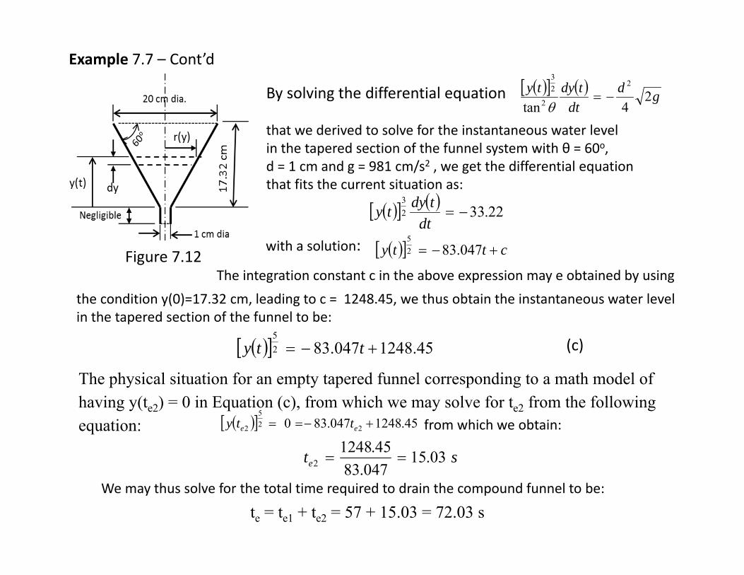
Example 7.7 – Cont’d

Figure 7.12

gddt

tdyty 24tan

2

2

23

By solving the differential equation

that we derived to solve for the instantaneous water level in the tapered section of the funnel system with θ = 60o, d = 1 cm and g = 981 cm/s2 , we get the differential equationthat fits the current situation as:

22.3323

dt

tdyty

with a solution: ctty 047.8325

The integration constant c in the above expression may e obtained by usingthe condition y(0)=17.32 cm, leading to c =  1248.45, we thus obtain the instantaneous water level in the tapered section of the funnel to be:

45.1248047.8325

tty

The physical situation for an empty tapered funnel corresponding to a math model of having y(te2) = 0 in Equation (c), from which we may solve for te2 from the following equation: 45.1248047.830 22

5

2 ee tty from which we obtain: 

ste 03.15047.83

45.12482

We may thus solve for the total time required to drain the compound funnel to be:

te = te1 + te2 = 57 + 15.03 = 72.03 s

(c)

Analysis on drainage of a funnel in winery: To design a funnel that will fill a wine bottlewith estimated time to fill the bottle

Bottle with given Geometry and

dimensions

?

?

?

Given

Given diameterMax space limit

Design objective: To provide SHORTEST time in draining the funnel for fastest bottling process

Example 7.8 

Design a circular funnel with a taper angle 60 degrees to fill the wine bottle described in Example 2.10 in Chapter 2 (P. 45).

The designer will configure and set the dimensions of the radius and the length H of the funnel with the diameter of the exit to be 1.5 cm, as illustrated in Figure 7.13 (a). Also determine the time required to fill the bottle with dimensions of the bottle as stipulated in Figure 2.33b.

(a) The wine bottle and funnel (b) Volume of a tapered funnel

Figure 7.13 Filling a wine bottle by a funnel 

(a) Determine the dimensions of the funnel: We will first set the volume of wine content in the bottle to be 841.52 cm3 as determined in Example 2.10.

Solution:

The purpose of this analysis is to design a funnel having the same volume as the bottle. 

Example 7.8‐ Cont’d 

To achieve this purpose, we will need to determine the maximum radius R of the funnel relating to the length H using the given taper angle of the funnel of θ = 60o. This can be done by the geometric relation of: tan60o = H/R, from which we get the following relationship of R and H as: 

R = H/tan60o = 0.577H                                      (a)

We will then determine both R and H for the funnel with a containment volume of 841.52 cm3.

By referring to Figure 7.13(b), we would have the volume of the funnel using Equation (2.17) with R(y) = 0.577y to be:

3

0

32

2

0

2

03485.0

3577.0577.0 HydyydyyRV

HHH

f

But the volume of the funnel = volume of the bottle, Vf = 0.3464 H3 = 841.52 cm3 which leads to the diameter of the funnel to be: D = 2R = 2x(0.577x13.416) = 15.4821 cm.

(b) Time required to drain the funnel (or time required to fill the bottle):Now that we have determined the geometry, the dimensions and the volume of the taperedfunnel, we may proceed to find the time required to drain this funnel as follows:

We may use Equation (7.20) to determine the required time to drain the tapered funnel. Thus, by substituting θ = 60o and d = 1.5 cm into Equation (7.20), we will have the differential equation for the instantaneous wine lever in the funnel y(t) during the drainage process to be:

981245.1

60tan

2

2

23

xdt

tdyxyo

or 7513.7423

dt

tdyty (b)

Example 7.8‐ Cont’d 

The solution y(t) of Equation (b) may be obtained by integrating both sides of Equation (b) resulting in:

[y(t)]2.5 = ‐186.8783t +C (c)

The integration constant c in Equation (c) may be determined with the initial condition of y(0) = H = 13.416 cm in Part (a) in the solution. We may thus obtain: c = 634.9654. 

The solution of the differential equation in (b) thus has the form of:

[y(t)]2.5 = ‐186.8783 t + 634.9654 (d)

If we let the time required to fill the wine bottle = te. This time te is the same as  the time required to empty the funnel. Consequently, we may obtain the value of te to be the required time to  drain the funnel and fill the wine bottle in Figure 7.13(a). We may thus solve for te from the following Equation (d) to give:

y(te) = ‐186.8783(te) + 634.9654 = 0 (e)

By solving te from Equation (e), we have the time required to fill the bottle to be: te = 3.42 s

7.5 Applications of First Order Differential Equations inHeat Transfer Analysis

Physics of heat transmission in substances in three(3) distinct modes:● Heat conduction in solids● Heat convection in fluids● Radiation of heat in space

Heat transfer in engineering analysis determines the temperature fields [or temperature distributions (or temperature variations)] in solid structures or fluids in engineering systems. Temperature fields in an engineering system can induce significant stresses, known as “thermal stresses” in which the temperature fields exist. Ignorance of these induced thermal stresses may cause overall failure of the engineering systems due to over‐stresses in the engineering systems.

Other significant consequences to structures or einginnering systems with excessive temperature effects may include: (1) significant deterioration of material properties (e.g., Young’s modulus, yield strength, ultimate tensile strength, etc.), at elevated temperatures, and (2) creep deformation of the materials –leading to creep failure ofstructure. Neither of these effects can be ignored in the engineering analyses.  

7.5.1 Fourier’s Law of Heat Conduction in Solids

Amount of heat flow, Q Q

d

Area, A

● Heat flows in SOLIDS by conduction● Heat flows from the part of solid at higher temperature toward the part with low temperature

- a situation similar to water flow from higher elevation to low elevation● Thus, there is definite relationship between the amount of heat flow (Q) and the temperature difference

(∆T) in the solid● Relating the Q and ∆T is what the Fourier’s law of heat conduction governs

Derivation of Fourier’s Law of Heat Conduction:Let us consider a solid slab: With its left surface maintained at temperature Ta and its right surface at Tb

Ta

Tb

Heat will flow from the left to the right surface if Ta > Tb

By observations, we can formulate the total amount of heat flow (Q)through the thickness of the slab relating to the following parameters:

dtTTAQ ba )(

Replacing the sign in the above expression by an = sign and a constant k, leads to:

dtTTAkQ ba )(

where A = the area to which heat flows; t = time allowing heat flow; and d = the distance of heat flow.

The constant k in Equation (7.21) is called “thermal conductivity” – treated as a property of the solid Material with a unit: Btu/in-s-oF in traditional system, or W/m-oC in the SI or metric system.

(7.21)

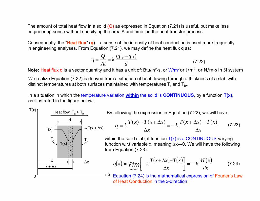
The amount of total heat flow in a solid (Q) as expressed in Equation (7.21) is useful, but make less engineering sense without specifying the area A and time t in the heat transfer process.

Consequently, the “Heat flux” (q) – a sense of the intensity of heat conduction is used more frequentlyin engineering analyses. From Equation (7.21), we may define the heat flux q as:

dTTk

AtQq ba )(

(7.22)

Note: Heat flux q is a vector quantity and it has a unit of: Btu/in2-s, or W/m2

We realize Equation (7.22) is derived from a situation of heat flowing through a thickness of a slab withdistinct temperatures at both surfaces maintained with temperatures Ta and Tb..

In a situation in which the temperature variation within the solid is CONTINUOUS, by a function T(x),as illustrated in the figure below:

T(x)

X

x

0

x + ∆x∆x

Ta Tb

T(x) T(x + ∆x)

Heat flow: Ta > Tb

T(x)

d

By following the expression in Equation (7.22), we will have:

xxTxxTk

xxxTxTkq

)()()()(

within the solid slab, if function T(x) is a CONTINUOUS varyingfunction w.r.t variable x, meaning ∆x→0, We will have the following from Equation (7.23):

(7.23)

dx

xdTkx

xTxxTkxq imx

0

(7.24)

Equation (7.24) is the mathematical expression of Fourier’s Law of Heat Conduction in the x-direction

or J/m2, or N/m‐s in SI system

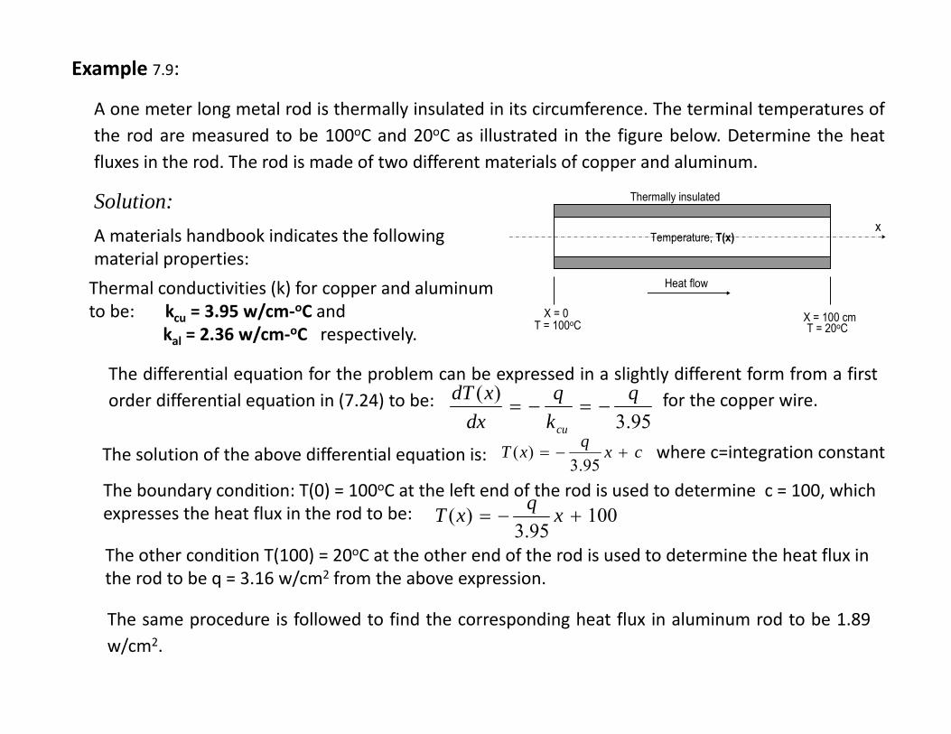
Example 7.9:

A one meter long metal rod is thermally insulated in its circumference. The terminal temperatures ofthe rod are measured to be 100oC and 20oC as illustrated in the figure below. Determine the heatfluxes in the rod. The rod is made of two different materials of copper and aluminum.

Temperature, T(x)

Thermally insulated

X = 0 X = 100 cm

x

T = 100oC T = 20oC

Heat flow

Solution:A materials handbook indicates the following material properties: Thermal conductivities (k) for copper and aluminum to be:       kcu = 3.95 w/cm‐oC and 

kal = 2.36 w/cm‐oC respectively.

The differential equation for the problem can be expressed in a slightly different form from a firstorder differential equation in (7.24) to be:

95.3)( q

kq

dxxdT

cu

for the copper wire. 

The boundary condition: T(0) = 100oC at the left end of the rod is used to determine  c = 100, which expresses the heat flux in the rod to be:

The solution of the above differential equation is: cxqxT 95.3

)( where c=integration constant

10095.3

)( xqxT

The other condition T(100) = 20oC at the other end of the rod is used to determine the heat flux in the rod to be q = 3.16 w/cm2 from the above expression.

The same procedure is followed to find the corresponding heat flux in aluminum rod to be 1.89w/cm2.

Example 7.10

Heat is transferred at the rate of 10 kW at the left end of a metal rod as shown in Figure 7.17.Determine the temperature distribution in the rod if the right end of the rod at x=2m is held at 50oC.  The cross sectional area of the rod  is 1200 mm2 and the thermal conductivity k = 100 kW/m‐oC

Temperature, T(x)

Thermally insulated

X = 0 X = 2 m

x

T(2m) = 50oC

Heat flow

Area, A = 1200 mm2

Heat Supply

= 10 Kw

Figure 7.17 Temperature Variation in a Metal Rod with Heat Flow

Solution:We have the total heat flow in the rod per unit time to be: dx

xdTkAqAQ )( (a)

with the end condition, T(x) = 50oC at x = 2 m (b)The temperature distribution T(x) in the rod may be obtained from the differential equation in Equation (a) in the following form:

mCxkA

Qdx

xdT o /33.83)101200(100

10)(6

(c)

Solving Equation (c) leads to the following relation: T(x) = -83.33x + cin which c is the integration constant to be determined by the end condition specified in Equation (b), resulting in a value of c = 216.67. We will thus have the temperature variation in the rod to be:

xxT 33.8367.216)(

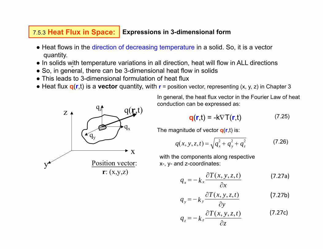
7.5.3 Heat Flux in Space:

-

Expressions in 3-dimensional form

xy

z q(r,t)

qxqy

qz

Position vector: r: (x,y,z)

● Heat flows in the direction of decreasing temperature in a solid. So, it is a vectorquantity.

● In solids with temperature variations in all direction, heat will flow in ALL directions● So, in general, there can be 3-dimensional heat flow in solids● This leads to 3-dimensional formulation of heat flux ● Heat flux q(r,t) is a vector quantity, with r = position vector, representing (x, y, z) in Chapter 3

q(r,t) = -kT(r,t)

In general, the heat flux vector in the Fourier Law of heat conduction can be expressed as:

(7.25)

The magnitude of vector q(r,t) is:

qqqtzyxq zyx222),,,(

with the components along respectivex-, y- and z-coordinates:

xtzyxT

kq xx

),,,(

ytzyxT

kq yy

),,,(

ztzyxT

kq zz

),,,(

(7.26)

(7.27a)

(7.27b)

(7.27c)

Examples of Heat Flux in a 2-D Plane

(1) Tubes with longitudinal fins are common in many tubular heat exchangers and boilers foreffective heat exchange between the hot fluids inside the tube and cooler fluids outside:

HOT

Cool The heat inside the tube (figure in the left) flows along the longitudinal plate‐fins to facilitate more effective cooling of the contacting fluid outside thetube.

It is desirable to analyze how effective heat can flow in the cross‐section of these longitudinal fins.

Hot

Cold

(2) Additional heat transfer areas (fins) attached to the exterior ofa motorcycle engine are also used to conduct excessive heatgenerated inside of the engine for better cooling effect ofthe a motorcycle engine by the outside cooling air:

Cooling fins

Cross-section of a tube withlongitudinal fins with onlyone fin shown

We have learned from Equation (7.21) that amount of heat flow in solids is proportional to the cross‐sectional area for heat transmission (A), which means that more heat can flow with more area for theheat flow. Following are two such examples for facilitating more heat flow in machines by adding more surface areas to facilitate more heat flow.

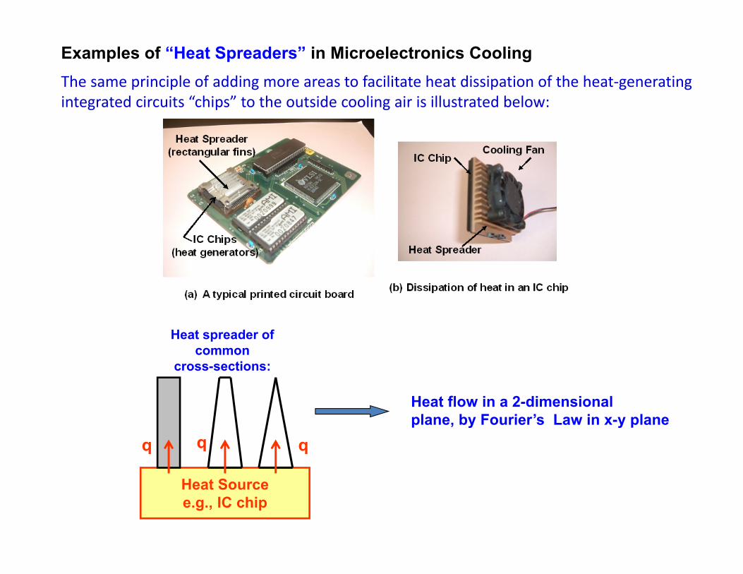
Examples of “Heat Spreaders” in Microelectronics Cooling

Heat Sourcee.g., IC chip

Heat spreader of common

cross-sections:

Heat flow in a 2-dimensionalplane, by Fourier’s Law in x-y plane

q q q

The same principle of adding more areas to facilitate heat dissipation of the heat‐generating integrated circuits “chips” to the outside cooling air is illustrated below: 

Mathematical formulation of Fourier’s Law of Heat Conduction in one- and 2-Dimensions

x

y q – heat flux in or out in the solid plane

T(x,y)Temp:

qx

qy

q(r,t) = ± kT(r,t)

For one-dimensional heat flow, Equation (7.24):

T(x) T(x)

dx

xdTkxq dx

xdTkxq

NOTE: The sign attached to q(x) changes with change of direction of heat flow!!

For two-dimensional heat flow, Equation (7.25):

Change of sign in the General form of Fourier’s Law of Heat Conduction:

Question: How to add a CORRECT sign in heat flux equations??

0 0

Guideline for Assigning Right Signs in Heat Flux Formulations in 2-D Planes:

x

y

q – heat flux in or out in the solid plane

T(x,y)Temp:

qx

qy

Outward NORMAL (n)(+VE) or (-ve)**

Sign of Outward Normal (n)? q along n? Sign of q in Fourier Law

+ Yes -+ No +- Yes +- No -

** OUTWARD NORMAL =Normal line pointing AWAYfrom the solid surface for heat flow

0

Example 7.12: Show the heat fluxes across the four edges of a rectangular block with +ve or –ve sign in terms of the available temperature distribution of T(x,y).

Given temp.T(x,y)

x

y q3

q2q1

q4

The specified directions of heat fluxes are prescribed as shownin the left figure. Thermal conductivity of the material k is given.

Solution:

Temperature in solid:T(x,y)

xyxTkq

),(

1

xyxTkq

),(

2

yyxTkq

),(

3

yyxTkq

),(

4

-n

-n

+n

+n

X

y

-noCase 4: -+yesCase 3: -

+noCase 2: +-yesCase 1: +

Sign of q in Fourier law

q along n?Sign of outward normal, n

-noCase 4: -+yesCase 3: -

+noCase 2: +-yesCase 1: +

Sign of q in Fourier law

q along n?Sign of outward normal, n

We may use the inserted table to express the heat fluxes q1, q2, q3 and q4 as shown in the following figure.

0

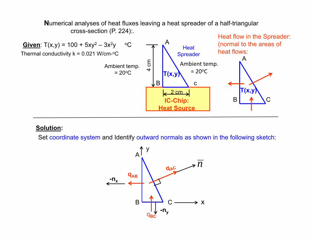
Numerical analyses of heat fluxes leaving a heat spreader of a half-triangular cross-section (P. 224):.

IC-Chip:Heat Source

HeatSpreader

Heat flow in the Spreader:(normal to the areas of heat flows:

A

cB

Ambient temp. = 20oC

Given: T(x,y) = 100 + 5xy2 – 3x2y oCThermal conductivity k = 0.021 W/cm-oC

T(x,y)

A

CB

qAB

qBC

Solution:

n

x

y

Set coordinate system and Identify outward normals as shown in the following sketch:

-nx

-ny

A

CBT(x,y)2 cm

4 cm Ambient temp. 

= 20oC

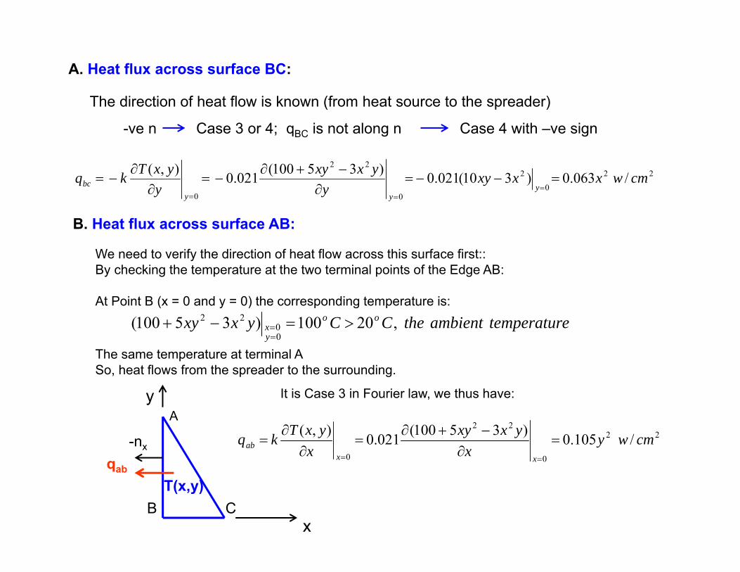
A. Heat flux across surface BC:

-ve n Case 3 or 4; qBC is not along n Case 4 with –ve sign

22

0

2

0

22

0

/063.0)310(021.0)35100(021.0),( cmwxxxyy

yxxyy

yxTkqy

yybc

B. Heat flux across surface AB:

The direction of heat flow is known (from heat source to the spreader)

We need to verify the direction of heat flow across this surface first::By checking the temperature at the two terminal points of the Edge AB:

At Point B (x = 0 and y = 0) the corresponding temperature is:

etemperaturambienttheCCyxxy oo

yx ,20100)35100(

00

22

The same temperature at terminal ASo, heat flows from the spreader to the surrounding.

CBT(x,y)

x

y

qab

-nx

It is Case 3 in Fourier law, we thus have:

22

0

22

0

/105.0)35100(021.0),( cmwyx

yxxyx

yxTkqxx

ab

A

C. Heat flux across surface AC:Surface AC is an inclined surface, so we need to handle this situation by the following procedure:

Use the same technique as in Case B, we may find the temperature at both terminal A and C to be 100oC > 20oC, the ambient temperature. So heat leaves the surface AC to the ambient.

n

BC

A

x

y

qac,x

qac,y

+nx

+ny

Based on the direction of the components of the heat flow and outward normal, we recognizeCase 1 for both qac,x and qac,y. Thus we have:

2

21

2

21

, /168.0)1220(021.0)65(021.0),( cmwxyyx

yxTkqyx

yx

xac

2

21

2

21

, /357.0)320(021.0)310(021.0),( cmwxxyy

yxTkqyx

yx

yac

and

The heat flux across the mid-point of surface AC at x = 1 cm and y = 2 cm is:

222,, /3945.0)357.0()168.0( cmwqqq yacxacac

Review of Newton’s Cooling Law for Heat Convection in Fluids

● Heat flows (transmission) in fluid by CONVECTION● Heat flows from higher temperature end to low temperature end in fluids● Motion of fluids causes heat convection ● As a rule-of-thumb, the amount of heat transmission by convection

is proportional to the velocity of the moving fluid

7.5.4 Mathematical expression of heat convection – The Newton’s Cooling Law

qA

B

TaTb

Ta > Tb

A fluid of non-uniform temperature in a container causes convective heat transfer:

Heat flows from Ta to Tb with Ta > Tb. The heat flux betweenA and B can be expressed by:

)()( baba TThTTq (7.28)

where h = heat transfer coefficient (W/m2-oC)

The heat transfer coefficient h in Equation (7.28) is normally determined by empirical expression,with its values relating to the Reynolds number (Re) of the moving fluid. The Reynolds number isexpressed as:

Lv

Rewith ρ = mass density of the fluid; L = characteristic length of thefluid flow, e.g., the diameter of a circular pipe, or the length of a flatplate; v = velocity of the moving fluid; μ = dynamic viscosity of the fluid

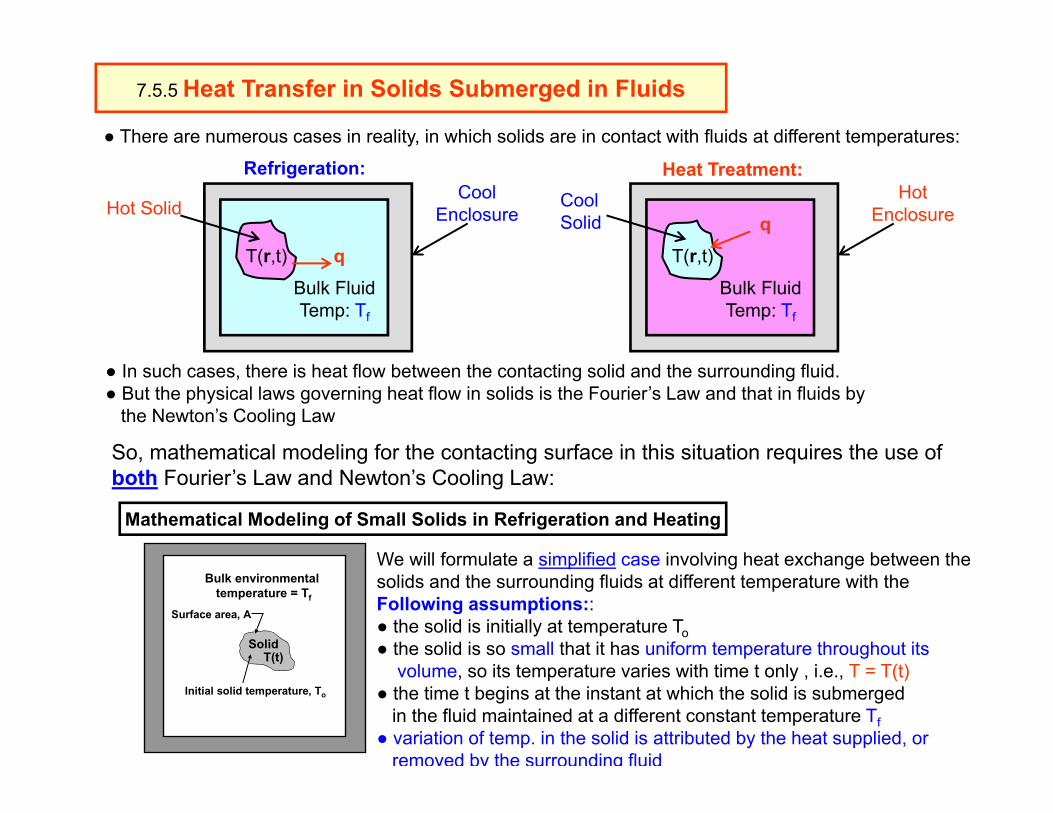
7.5.5 Heat Transfer in Solids Submerged in Fluids

● There are numerous cases in reality, in which solids are in contact with fluids at different temperatures:

● In such cases, there is heat flow between the contacting solid and the surrounding fluid.● But the physical laws governing heat flow in solids is the Fourier’s Law and that in fluids by

the Newton’s Cooling Law

T(r,t)Bulk FluidTemp: Tf

q

CoolEnclosureHot Solid

So, mathematical modeling for the contacting surface in this situation requires the use of both Fourier’s Law and Newton’s Cooling Law:

Bulk environmental temperature = Tf

Surface area, A

SolidT(t)

Initial solid temperature, To

We will formulate a simplified case involving heat exchange between the solids and the surrounding fluids at different temperature with theFollowing assumptions::● the solid is initially at temperature To● the solid is so small that it has uniform temperature throughout its

volume, so its temperature varies with time t only , i.e., T = T(t)● the time t begins at the instant at which the solid is submerged

in the fluid maintained at a different constant temperature Tf● variation of temp. in the solid is attributed by the heat supplied, or

removed by the surrounding fluid

T(r,t)Bulk FluidTemp: Tf

qHot

EnclosureCoolSolid

Refrigeration: Heat Treatment:

Mathematical Modeling of Small Solids in Refrigeration and Heating

Bulk environmental temperature = Tf

Surface area, A

SolidT(t)

Initial solid temperature, To

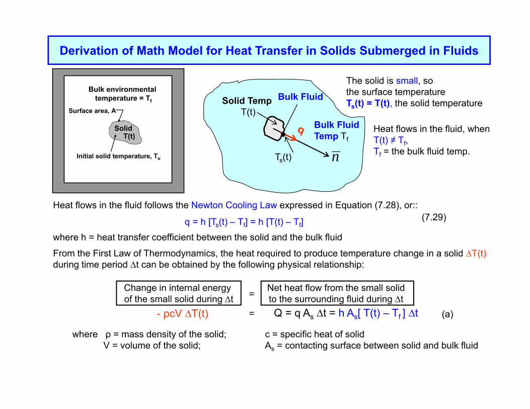
Derivation of Math Model for Heat Transfer in Solids Submerged in Fluids

nTs(t)

Bulk FluidTemp Tf

Bulk FluidSolid TempT(t)

The solid is small, so the surface temperature Ts(t) = T(t), the solid temperature

Heat flows in the fluid, whenT(t) ≠ Tf, Tf = the bulk fluid temp.

From the First Law of Thermodynamics, the heat required to produce temperature change in a solid ∆T(t)during time period ∆t can be obtained by the following physical relationship:

Heat flows in the fluid follows the Newton Cooling Law expressed in Equation (7.28), or::

q = h [Ts(t) – Tf] = h [T(t) – Tf](7.29)

where h = heat transfer coefficient between the solid and the bulk fluid

Change in internal energy of the small solid during ∆t = Net heat flow from the small solid

to the surrounding fluid during ∆t= Q = q As ∆t = h As[ T(t) – Tf ] ∆t- ρcV ∆T(t)

where ρ = mass density of the solid; c = specific heat of solidV = volume of the solid; As = contacting surface between solid and bulk fluid

(a)

From Equation (a), we express the rate of temperature change in the solid to be:

fs TtTAVc

httT

(b)

Since h , ρ, c and V on the right-hand-side of Equation (b) are constants, we may lump these constants to let:

Vch

with a unit (/m2-s)

Equation (b) is thus expressed as: fs TtTAttT

(7.30)

Since the change of the temperature of the submerged solid T(t) is CONTINOUS with respect to time t,i.e., ot , and if we replace the contact surface area As to a generic symbol A, we can express

Equation (3.27) in the form of a 1st order differential equation as follows::

fTtTAdt

tdT (7.31)

with a given initial condition: 00ToTtT

t

Bulk environmental temperature = Tf

Surface area, A

SolidT(t)

Initial solid temperature, To

(7.27)

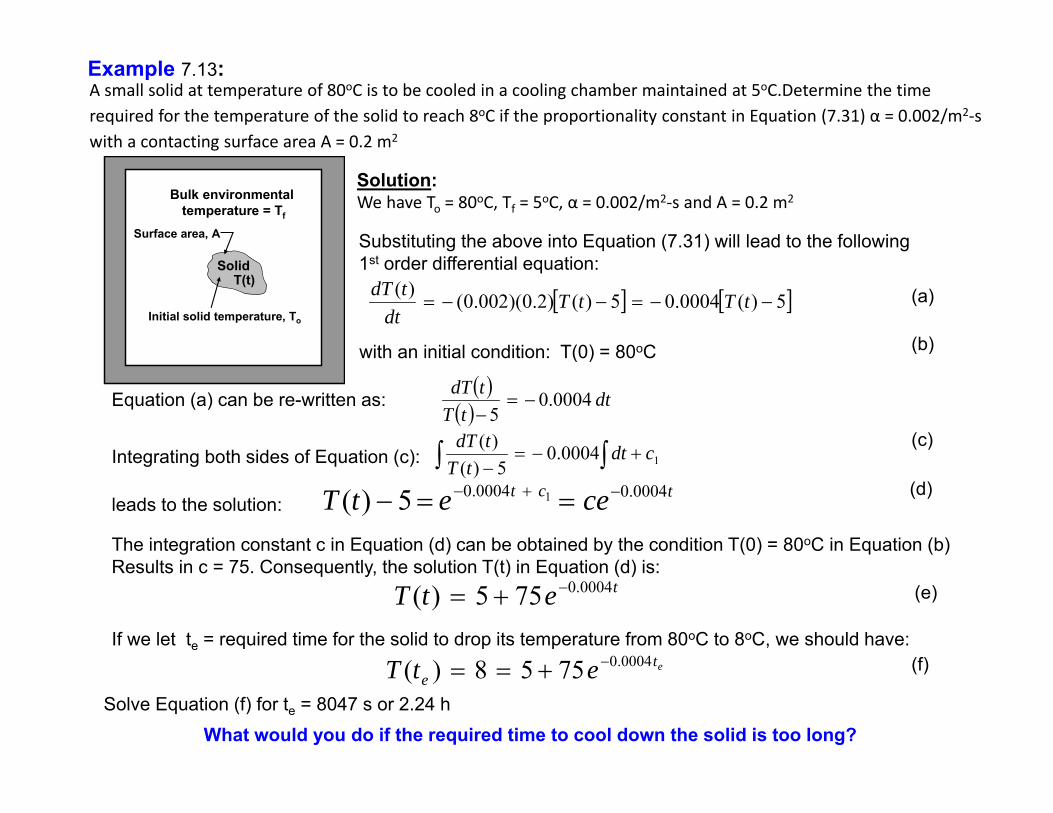
Example 7.13:

Bulk environmental temperature = Tf

Surface area, A

SolidT(t)

Initial solid temperature, To

Solution:We have To = 80oC, Tf = 5oC, α = 0.002/m2‐s and A = 0.2 m2

Substituting the above into Equation (7.31) will lead to the following 1st order differential equation:

5)(0004.05)()2.0)(002.0()( tTtT

dttdT (a)

with an initial condition: T(0) = 80oC (b)

Equation (a) can be re-written as:

dttT

tdT 0004.05

Integrating both sides of Equation (c): 10004.0

5)()( cdt

tTtdT (c)

leads to the solution:tct ceetT 0004.00004.0 15)( (d)

The integration constant c in Equation (d) can be obtained by the condition T(0) = 80oC in Equation (b)Results in c = 75. Consequently, the solution T(t) in Equation (d) is:

tetT 0004.0755)( (e)

If we let te = required time for the solid to drop its temperature from 80oC to 8oC, we should have:et

e etT 0004.07558)( (f)

Solve Equation (f) for te = 8047 s or 2.24 hWhat would you do if the required time to cool down the solid is too long?

A small solid at temperature of 80oC is to be cooled in a cooling chamber maintained at 5oC.Determine the time required for the temperature of the solid to reach 8oC if the proportionality constant in Equation (7.31) α = 0.002/m2‐s with a contacting surface area A = 0.2 m2

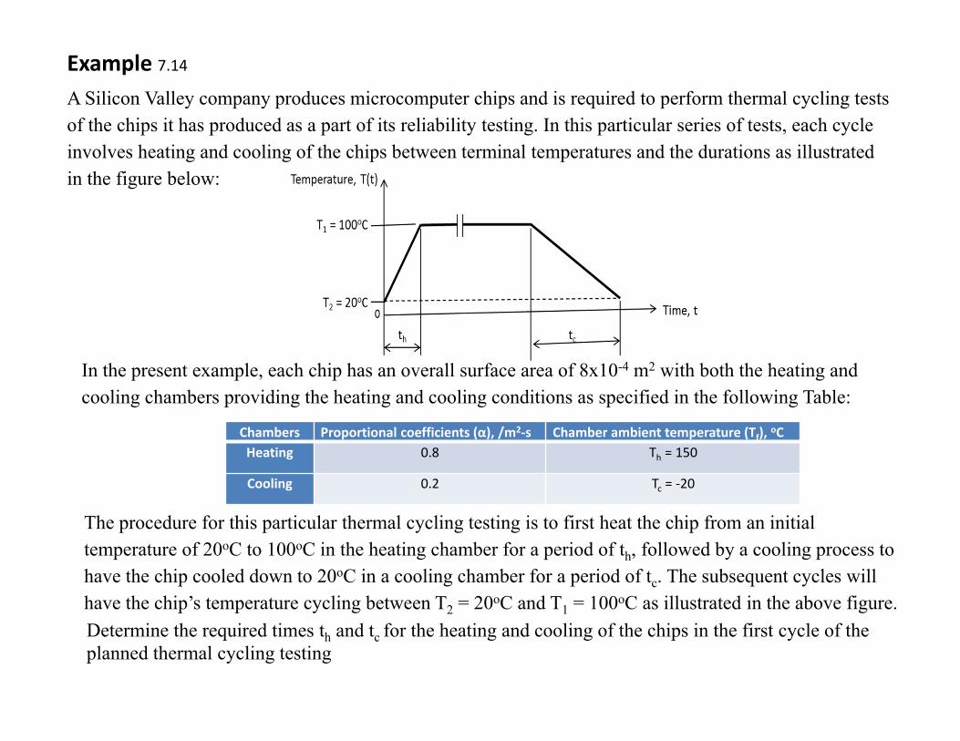
Example 7.14

A Silicon Valley company produces microcomputer chips and is required to perform thermal cycling tests of the chips it has produced as a part of its reliability testing. In this particular series of tests, each cycle involves heating and cooling of the chips between terminal temperatures and the durations as illustrated in the figure below:

In the present example, each chip has an overall surface area of 8x10-4 m2 with both the heating and cooling chambers providing the heating and cooling conditions as specified in the following Table:

Chambers Proportional coefficients (α), /m2‐s Chamber ambient temperature (Tf), oCHeating 0.8 Th = 150

Cooling 0.2 Tc = ‐20

The procedure for this particular thermal cycling testing is to first heat the chip from an initial temperature of 20oC to 100oC in the heating chamber for a period of th, followed by a cooling process to have the chip cooled down to 20oC in a cooling chamber for a period of tc. The subsequent cycles will have the chip’s temperature cycling between T2 = 20oC and T1 = 100oC as illustrated in the above figure.Determine the required times th and tc for the heating and cooling of the chips in the first cycle of the planned thermal cycling testing

Solution:Example 7.14‐Cont’d

(A) For the heating portion of the thermal cycling test:

We will use the first order differential equation in Equation (7.31) to solve the instantaneous temperature in the chip T(t) as follows:

150104.6 4 tTxdt

tdT (a)

We have from conditions Table the values of α = 0.8/m2-s and Tf = 150oC together with A = 8x10-4

m2 and the initial temperature of the chip T0 = 20oC. Substituting these given conditions into Equation (a) will result in the following differential equation for the solution T(t):

150104.6 4 tTxdt

tdT (b)

with condition:  200 00

TTtT

t(c)

By integrating both sides of the Equation (b), we get:

1

4104.6150

cdtxtT

tdT (d)

The integration constant c1 is determined by the initial condition in Equation (c). We thus obtain the following expression for function T(t) as:

1501304104.6 txetT

(e)

The time required to heat the chips to 100oC may be determined by the relation that T(th) = T1 = 100oC, which will lead to the following expression:

The time required to heat the chips to 100oC may be determined by the relation that T(th) = T1 = 100oC, which will lead to the following expression: 150130100

4104.6104.6 h

x txe

min88.241493104.6

130100150

4 orsx

nth

from which we solve for

Example 7.14‐Cont’d

(b) For the cooling portion of the thermal cycling:

We have the proportional coefficient α = 0.2 /m2‐s and Tf = ‐20oC in the cooling process

We will use the same Equation (a) for the solution T(t) with the following expression: 20106.1201082.0 44 tTxtTxx

dttdT (f)

The solution of T(t) in Equation (f) has the following form: 2

4106.120 ctxtTn

In which c2 is the integration constant to be determined by the initial condition of  CTTtT o

t1000 10

, from which we have c2 = 4.7875. We thus have the solution:

201204106.1 txetT (g)

from which we may express the temperature of the chip at time tc to be:

20120204106.1 ctx

c etT

Solve for tc from the above equation and obtain tc = 6813 s or 113.55 minutes or 1.89 hour.

(c) Two options to shorten the times for heating and cooling: (a) For shortening time for heating: One may increase both the α-values and the bulk fluid temperature tf, and (b) for shortening the time for cooling would involve increasing the α-values but lower the bulk fluid temperature tf. Both options will increase the cost for the testing because increasing α-values in the heating or cooling chambers require increasing the speed of bulk fluid moving over the solid surfaces, and increasing thand reducing tc in the chambers can also be costly too.

7.6 Rigid Body Dynamics Under the Influence of Gravitation

We will demonstrate the application of 1st order differential equationin rigid body dynamics using Newton’s Second Law

∑F = ma

where F = induced dynamic force on the moving solids, M = the mass of the solids, and a = the accelerations or decelerations of the moving solids

Rigid Body Motion Under Strong Influence of Gravitation:

There are many engineering systems that involve dynamic behavior under strong influence of Gravitational acceleration of decelerations such as described in Section 3.73, or in the moving Solids in the flowing lustrations:

Rocket launch The helicopter

The paratroopers

Observation on A Rigid Body in Motion Under Influence of Gravitation

Galileo Galilei

Galileo’s free-fall experimentfrom the leaning tower inPisa, Italy, December 1612

X

R(t)R(t)

W W

F(t)F(t)

Velocity v(t)Velocity v(t)

Free Fall Thrown-up

X = 0

Math

Modeling

Solution sought:● The instantaneous position x(t) at time t● The instantaneous velocity v(t)● The maximum height the body can reach, and the required time

with initial velocity vo in the “thrown-up” situation

These solutions can be obtained by first deriving the mathematical expression (a differential equationin this case), and solve for the solutions

By kinematics of a moving solid:If the instantaneous position of the solid is expressed as x(t), we will have:

dttdxtv to be the

instantaneous velocity, and dt

tdvta to be the instantaneous acceleration (or deceleration)

(acceleration bygravitation)

(Deceleration byGravitation)

X

R(t)

W

F(t)

Velocity v(t)

Thrown-up

X = 0

Case A: Throw-up of a solid with initial velocity vo:

The forces acting on the up-moving solid should be in equilibrium at time t:

By using a sign convention of forces along +ve x-axis being +ve for the forces, we have:

∑ Fx = 0which leads to:

∑ Fx = -W - R(t) - F(t) = 0

with W = mg, R(t) = cv(t), and dt

tdvmtamtF

A 1st order differential equation is obtained:

gtvmc

dttdv

)()((7.32)

with an initial condition:

otvvtv

0

0(a)

The solution of Equation (7.32) is obtained by comparing it with the typical 1st order differential equation in Equation (7.6) with solution in Equation (7.7) shown below:

)(

)()()(

1)(tF

KdttgtFtF

tv

)()()()( tgtutpdt

tdv

with a solution:

(7.6)

(7.7)

The present case has:

dttpetF

)()( gtgand

mctp )()(,

Consequently, the solution of Equation (7.32) has the form:

tmc

mct

mct

mct Ke

cmg

e

Kdtgee

tv

1)(

(7.33)

In which the constant K is determined by the given initial condition in Equation (a), with:

cmgvK o

The complete solution of Equation (7.32) with the substitution of K in Equation (b) into Equation (3.26) forThe instantaneous velocity of the rising solid:

(b)

tmc

o ec

mgvc

mgtv

)( (7.34)

Case A: Throw‐up of a solid with initial velocity vo – Cont’d:

Case A: Throw‐up of a solid with initial velocity vo – Cont’d:

The other solution that engineers often sought in this case is: “How long would it take for this solid reaching the maximum height and the time required to reach this stage:

We realize the fact that the solid will reduce it velocity continuously on its way up, untilit reaches the maximum height, at which point the velocity will reach a zero value. Mathematically, we will have a condition that v(tm) = 0 in which tm is the required timefor the upward moving solid reaching its maximum height. We thus have the following expression:

mtmc

o ec

mgvc

mg

0

from which, we solve for tm to be:

=  1 (7.35)

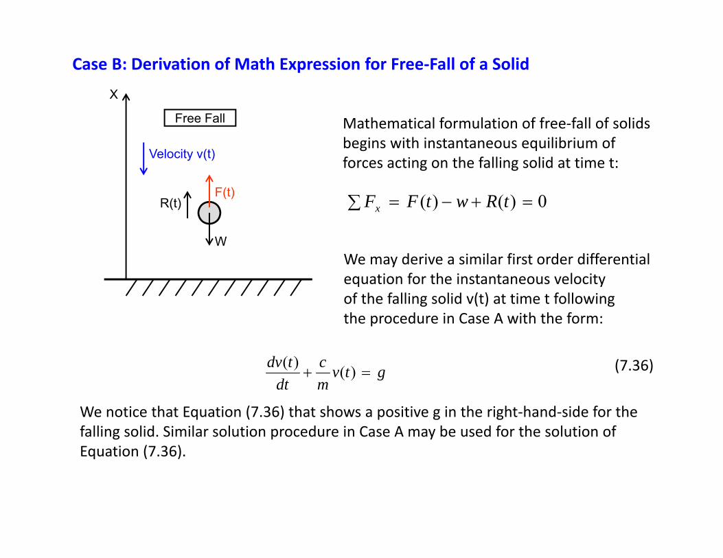
Mathematical formulation of free‐fall of solids begins with instantaneous equilibrium of forces acting on the falling solid at time t:

Case B: Derivation of Math Expression for Free‐Fall of a Solid 

0)()( tRwtFFx

We may derive a similar first order differential equation for the instantaneous velocity of the falling solid v(t) at time t following the procedure in Case A with the form: 

gtvmc

dttdv

)()( (7.36)

We notice that Equation (7.36) that shows a positive g in the right‐hand‐side for the falling solid. Similar solution procedure in Case A may be used for the solution of Equation (7.36).

R(t)

W

F(t)

Velocity v(t)

Free Fall

X

Example 7.15: A case illustration of Free‐fall of a solid:

An armed paratrooper with ammunition weighing 322 pounds jumps from a plane with zero initial velocity, as shown in the figure in the right.  

We assume that the troopers encountered negligible side wind in their descending. However, they encounter an air resistance that is 15 times the square of the descending velocity v(t), i.e., 15[v(t)]2. 

Determine the following: 

(a) Derive the appropriate equation for the instantaneous descending velocity v(t), (b) Solve the equation for the descending velocity. (c) Estimate the time required for the paratrooper to reach the ground from a height 

of 10,000 feet.(d) Estimate the impact velocity of the paratrooper upon touching the ground, and 

the corresponding momentum.

Example 7.15 – Cont’d

Solution:

(a) Derivation of the  differential equation:

The total mass of the falling body m = 322/32.2 = 10 slugs, the air resistance R(t) = cv(t) = 15[v(t)]2 

The instantaneous descending velocity v(t) can be obtained by using Equation (7.36) as:

2.3210

)(15)( 2

tv

dttdv (a)

or in the form: 2)(15322)(10 tvdt

tdv (b)

with the initial condition:  000

vtvt

(c)

(b) Solution for instantaneous velocity v(t):Equation (b) may be expressed in the form after being separated for the solution:

dtdvv

21532210

where the instantaneous descending velocity of the trooper v=v(t)

(d)

ctvv

634.4634.4log

13910

Integrating both sides of Equation (d) will result in:(e)

The integration constant c in Equation (e) can e determined by the initial condition in Equation (c) resulting in c=0. We thus have the solution v(t) to be: 1

)1(634.4)( 9.13

9.13

t

t

eetv (f)

Example 7.15 – Cont’d

(c) Estimate the time required for the paratrooper to reach the ground from a height of 10,000 feet:

Let the descending distance of the paratrooper to be X(t), in which t is the time starting from the moment of his jumping out the carrier airplane. The expression

dttdXtv )()( leads to the following expression for the

distance of descending by the paratrooper: dttvtX

t

0

(g)

ttt

t

t

tendte

etX0

9.13

0 9.13

9.13

634.41667.01

1634.4

After we fill Equation with v(t) in Equation (f) and get the above integral for the distance that the trooper had traveled at time t to be:

X(t) = 0.6667ℓn (1+e 13.9t) -4.634t – 0.4621 (h)

Let tg be the required time to travel a distance 10,000 feet, we will have the following relationship:10000 = 0.6667ℓn (1+e 13.9tg) -4.634tg – 0.4621 (j)

Equation (j) will provide us with an approximate value of tg = 2158.46 s 0r 35.95 minutes

(d) Estimate the impact velocity of the paratrooper upon touching the ground, and the corresponding momentum:

sfte

eV x

x

f /634.41

1634.446.21589.13

46.21589.13

We may compute the terminal velocity of the trooper to  be:

,which leads to the impact momentum to be: mv(tg) = 46.34 ft‐lb