Chapter 7: Eligibility Traces - UMass Amherst

R. S. Sutton and A. G. Barto: Reinforcement Learning: An Introduction 1

Chapter 7: Eligibility Traces


Midterm

Mean = 77.33 Median = 82


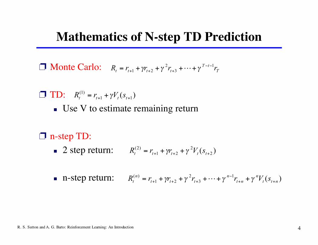
N-step TD Prediction

❐ Idea: Look farther into the future when you do TD backup(1, 2, 3, …, n steps)


❐ Monte Carlo:

❐ TD: Use V to estimate remaining return

❐ n-step TD: 2 step return:

n-step return:

Mathematics of N-step TD Prediction

T

tT

ttttrrrrR1

3

2

21

!!

+++ ++++= """ L

)( 11

)1(

++ +=ttttsVrR !

)( 2

2

21

)2(

+++ ++=tttttsVrrR !!

)(1

3

2

21

)(

ntt

n

nt

n

ttt

n

tsVrrrrR ++

!

+++ +++++= """" L


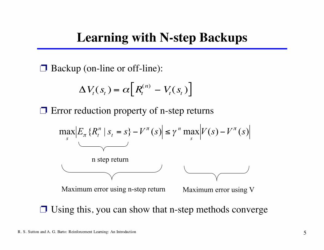
Learning with N-step Backups

❐ Backup (on-line or off-line):

❐ Error reduction property of n-step returns

❐ Using this, you can show that n-step methods converge

)()(max)(}|{max sVsVsVssREs

n

t

n

ts

!!

! " #$#=

n step return

Maximum error using n-step return Maximum error using V

!Vt(s

t) = " R

t

(n)# V

t(s

t)[ ]


Random Walk Examples

❐ How does 2-step TD work here?❐ How about 3-step TD?


A Larger Example

❐ Task: 19 staterandom walk

❐ Do you think thereis an optimal n (foreverything)?


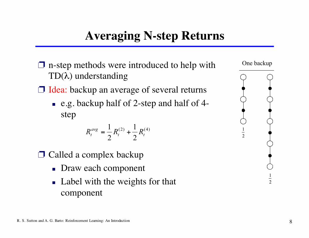
Averaging N-step Returns

❐ n-step methods were introduced to help withTD(λ) understanding

❐ Idea: backup an average of several returns e.g. backup half of 2-step and half of 4-

step

❐ Called a complex backup Draw each component Label with the weights for that

component

)4()2(

2

1

2

1tt

avg

t RRR +=

One backup


Forward View of TD(λ)

❐ TD(λ) is a method foraveraging all n-step backups weight by λn-1 (time since

visitation) λ-return:

❐ Backup using λ-return:

Rt

!= (1" ! ) !

n "1

n=1

#

$ Rt

(n)

!Vt(s

t) = " R

t

#$ V

t(s

t)[ ]


λ-return Weighting Function


Relation to TD(0) and MC

❐ λ-return can be rewritten as:

❐ If λ = 1, you get MC:

❐ If λ = 0, you get TD(0)

Rt

!= (1" ! ) !

n"1

n=1

T" t"1

# Rt

(n)+ !

T"t"1Rt

Rt

!= (1"1) 1

n"1

n=1

T"t"1

# Rt

(n )+ 1

T" t"1Rt= R

t

Rt

!= (1" 0) 0

n"1

n=1

T"t"1

# Rt

(n )+ 0

T" t"1Rt= R

t

(1)

Until termination After termination


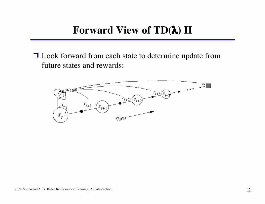
Forward View of TD(λ) II

❐ Look forward from each state to determine update fromfuture states and rewards:


λ-return on the Random Walk

❐ Same 19 state random walk as before❐ Why do you think intermediate values of λ are best?


Backward View of TD(λ)

❐ The forward view was for theory❐ The backward view is for mechanism

❐ New variable called eligibility trace On each step, decay all traces by γλ and increment the

trace for the current state by 1 Accumulating trace

+!")(set

et(s) =

!"et#1(s) if s $ s

t

!"et#1(s) +1 if s = s

t

% & '


On-line Tabular TD(λ)

Initialize V(s) arbitrarily and e(s) = 0, for all s !S

Repeat (for each episode) :

Initialize s

Repeat (for each step of episode) :

a" action given by # for s

Take action a, observe reward, r, and next state $ s

% " r +&V( $ s ) ' V (s)

e(s)" e(s) +1

For all s :

V(s) "V(s) +(%e(s)

e(s) "&)e(s)

s" $ s

Until s is terminal


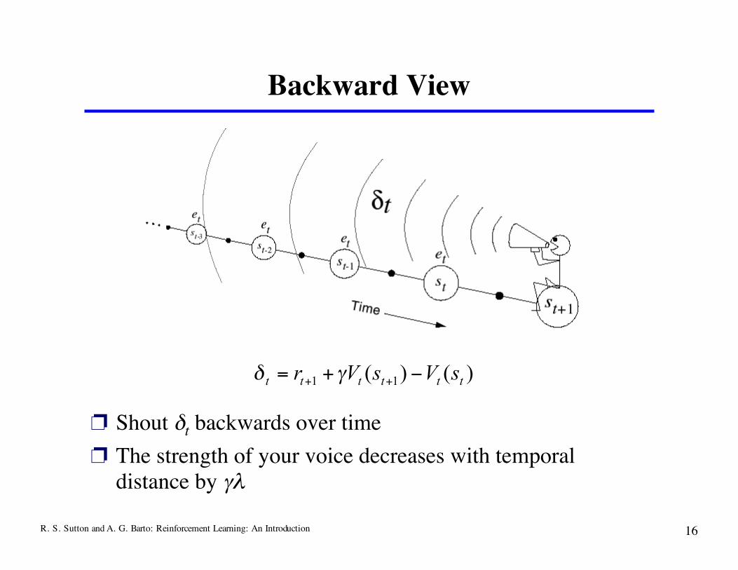
Backward View

❐ Shout δt backwards over time❐ The strength of your voice decreases with temporal

distance by γλ

)()( 11 ttttttsVsVr !+= ++ "#


Relation of Backwards View to MC & TD(0)

❐ Using update rule:

❐ As before, if you set λ to 0, you get to TD(0)❐ If you set λ to 1, you get MC but in a better way

Can apply TD(1) to continuing tasks Works incrementally and on-line (instead of waiting to

the end of the episode)

)()( sesVttt

!"=#


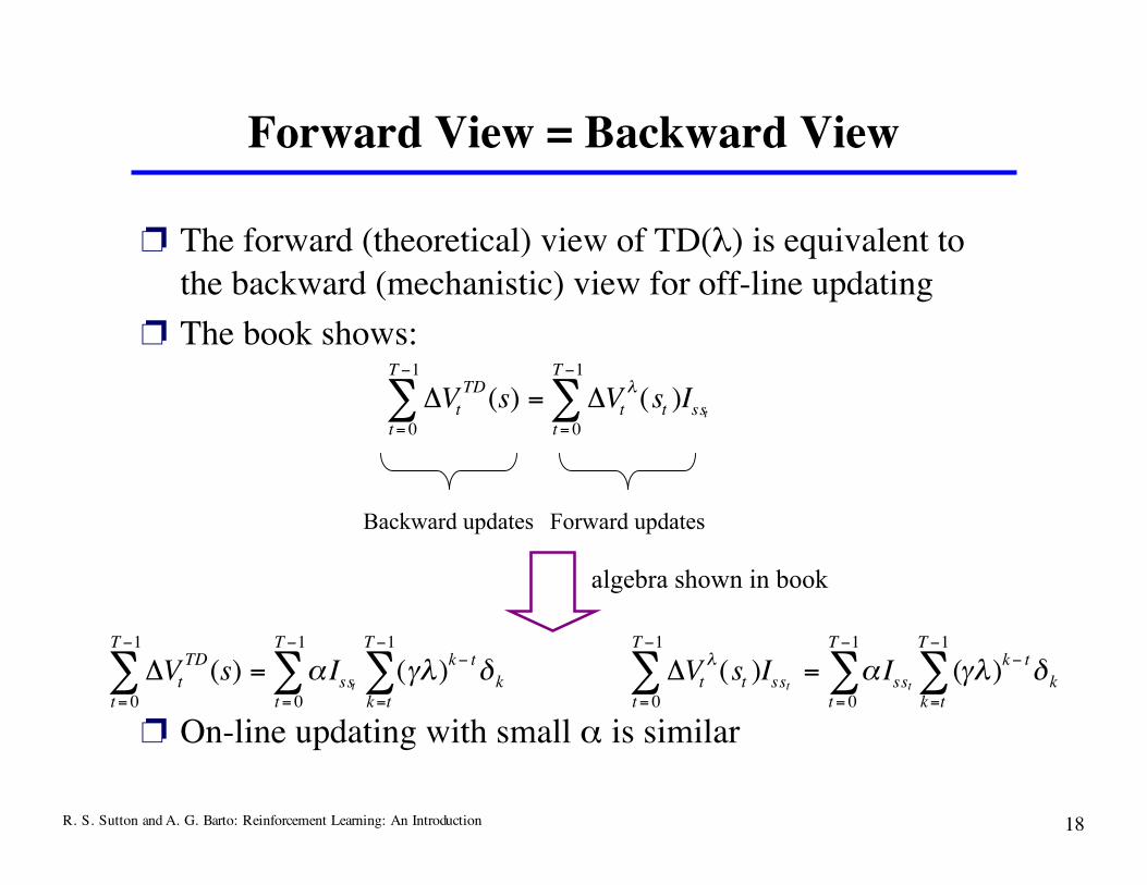
Forward View = Backward View

❐ The forward (theoretical) view of TD(λ) is equivalent tothe backward (mechanistic) view for off-line updating

❐ The book shows:

❐ On-line updating with small α is similar

!Vt

TD(s)

t= 0

T"1

# = $t= 0

T"1

# Isst

(%&)k" t'k

k=t

T"1

# !Vt

"(s

t)Isst

t= 0

T#1

$ = %t= 0

T#1

$ Isst

(&")k# t'k

k=t

T#1

$

!Vt

TD

(s)t= 0

T"1

# = !Vt

$(s

t)

t= 0

T"1

# Isst

Backward updates Forward updates

algebra shown in book


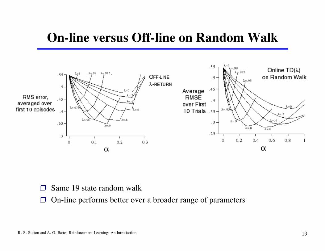
On-line versus Off-line on Random Walk

❐ Same 19 state random walk❐ On-line performs better over a broader range of parameters


Control: Sarsa(λ)

❐ Save eligibility for state-actionpairs instead of just states

et(s, a) =

!"et#1(s, a) +1 if s = s

t and a = a

t

!"et#1(s,a) otherwise

$ % &

Qt+1(s, a) = Q

t(s, a) +'(

tet(s, a)

(t

= rt+1 + !Q

t(s

t+1,at+1) #Qt(s

t, a

t)


Sarsa(λ) Algorithm

Initialize Q(s,a) arbitrarily and e(s, a) = 0, for all s, a


Initialize s, a


Take action a, observe r, ! s

Choose ! a from ! s using policy derived from Q (e.g. ? - greedy)

" # r +$Q( ! s , ! a ) %Q(s, a)

e(s,a)# e(s,a) +1

For all s,a :

Q(s, a)#Q(s, a) +&"e(s, a)

e(s, a) #$'e(s, a)

s# ! s ;a # ! a

Until s is terminal


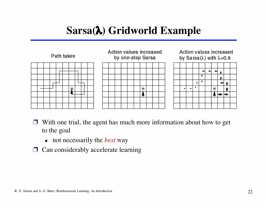
Sarsa(λ) Gridworld Example

❐ With one trial, the agent has much more information about how to getto the goal not necessarily the best way

❐ Can considerably accelerate learning


Three Approaches to Q(λ)

❐ How can we extend this to Q-learning?

❐ If you mark every state actionpair as eligible, you backupover non-greedy policy Watkins: Zero out

eligibility trace after a non-greedy action. Do maxwhen backing up at firstnon-greedy choice.

et(s, a) =

1 + !"et#1(s, a)

0

!"et#1(s,a)

if s = st, a = a

t,Q

t#1(st,a

t) = max

aQ

t#1(st, a)

if Qt#1(st

,at) $ max

aQ

t#1(st,a)

otherwise

%

& '

( '

Qt +1(s, a) = Q

t(s, a) +)*

te

t(s, a)

*t

= rt +1 + ! max + a

Qt(s

t +1, + a ) #Qt(s

t,a

t)


Watkins’s Q(λ)

Initialize Q(s,a) arbitrarily and e(s, a) = 0, for all s, a


Initialize s, a


Take action a, observe r, ! s

Choose ! a from ! s using policy derived from Q (e.g. ? - greedy)

a* " arg maxb Q( ! s , b) (if a ties for the max, then a* " ! a )

# " r +$Q( ! s , ! a ) %Q(s, a*)

e(s,a)" e(s,a) +1

For all s,a :

Q(s, a)"Q(s, a) +&#e(s, a)

If ! a = a*, then e(s, a) "$'e(s,a)

else e(s, a)" 0

s" ! s ;a " ! a

Until s is terminal


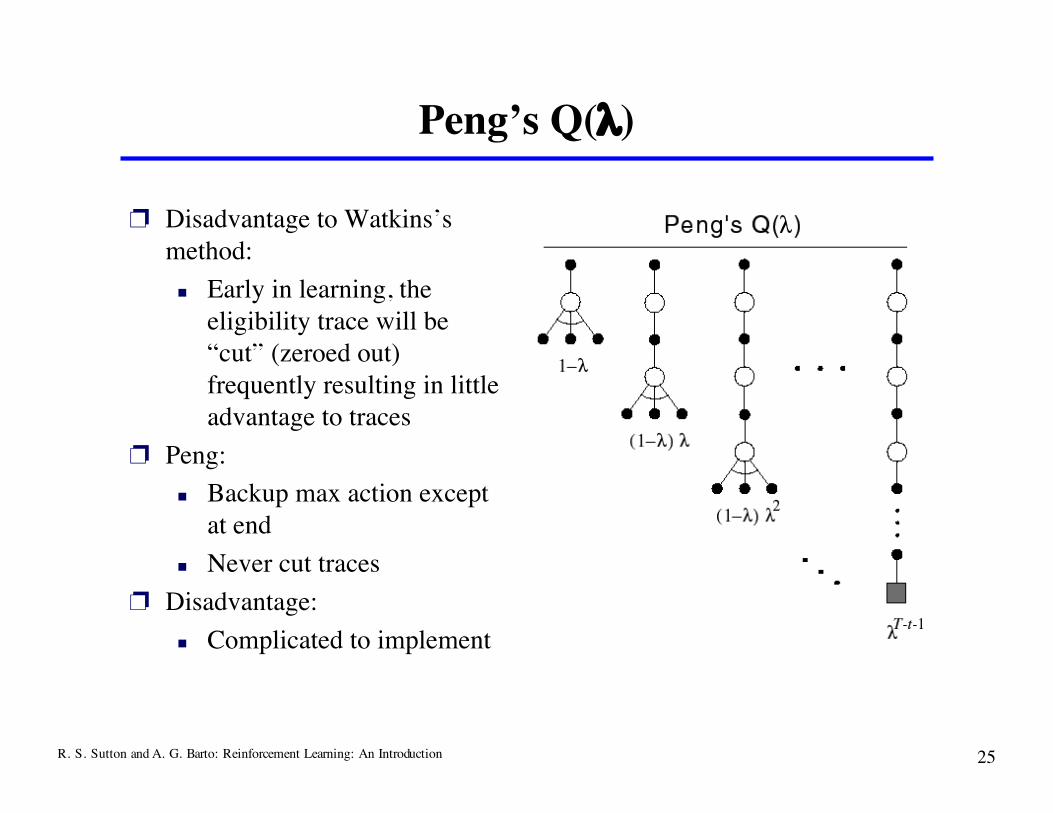
Peng’s Q(λ)

❐ Disadvantage to Watkins’smethod: Early in learning, the

eligibility trace will be“cut” (zeroed out)frequently resulting in littleadvantage to traces

❐ Peng: Backup max action except

at end Never cut traces

❐ Disadvantage: Complicated to implement


Naïve Q(λ)

❐ Idea: is it really a problem tobackup exploratory actions? Never zero traces Always backup max at

current action (unlike Pengor Watkins’s)

❐ Is this truly naïve?❐ Works well is preliminary

empirical studies

What is the backup diagram?


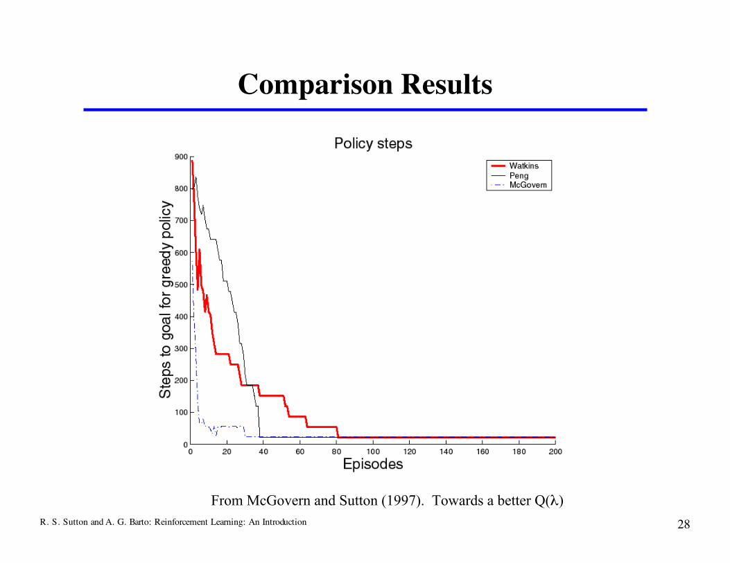
Comparison Task

From McGovern and Sutton (1997). Towards a better Q(λ)

❐ Compared Watkins’s, Peng’s, and Naïve (calledMcGovern’s here) Q(λ) on several tasks. See McGovern and Sutton (1997). Towards a Better Q(λ) for other tasks and results (stochastic tasks,continuing tasks, etc)

❐ Deterministic gridworld with obstacles 10x10 gridworld 25 randomly generated obstacles 30 runs α = 0.05, γ = 0.9, λ = 0.9, ε = 0.05, accumulating traces


Comparison Results

From McGovern and Sutton (1997). Towards a better Q(λ)


Convergence of the Q(λ)’s

❐ None of the methods are proven to converge. Much extra credit if you can prove any of them.

❐ Watkins’s is thought to converge to Q*

❐ Peng’s is thought to converge to a mixture of Qπ and Q*

❐ Naïve - Q*?


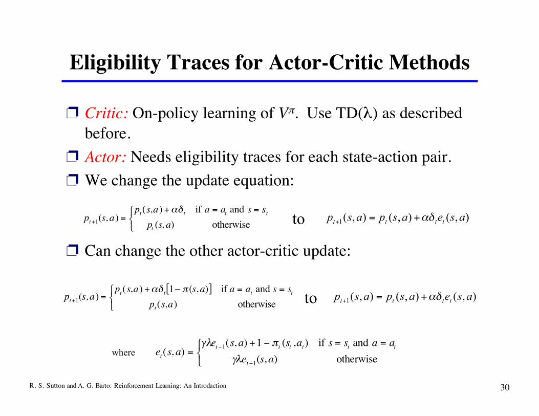
Eligibility Traces for Actor-Critic Methods

❐ Critic: On-policy learning of Vπ. Use TD(λ) as describedbefore.

❐ Actor: Needs eligibility traces for each state-action pair.❐ We change the update equation:

❐ Can change the other actor-critic update:

pt+1(s, a) =pt(s,a) +!" t if a = at and s = st

pt (s, a) otherwise

# $ %

),(),(),(1 aseaspasptttt

!"+=+to

pt+1(s, a) =pt(s,a) +!" t 1# $ (s, a)[ ] if a = at and s = st

pt(s,a) otherwise

% & '

to ),(),(),(1 aseaspasptttt

!"+=+

et(s, a) =

!"et#1(s, a) +1 # $

t(st,a

t) if s = s

t and a = a

t

!"et#1(s, a) otherwise

% & '

where


Replacing Traces

❐ Using accumulating traces, frequently visited states canhave eligibilities greater than 1 This can be a problem for convergence

❐ Replacing traces: Instead of adding 1 when you visit astate, set that trace to 1

et(s) =

!"et#1(s) if s $ s

t

1 if s = st

% & '


Replacing Traces Example

❐ Same 19 state random walk task as before❐ Replacing traces perform better than accumulating traces over more

values of λ


Why Replacing Traces?

❐ Replacing traces can significantly speed learning

❐ They can make the system perform well for a broader set ofparameters

❐ Accumulating traces can do poorly on certain types of tasks

Why is this task particularly onerousfor accumulating traces?


More Replacing Traces

❐ Off-line replacing trace TD(1) is identical to first-visit MC

❐ Extension to action-values: When you revisit a state, what should you do with the

traces for the other actions? Singh and Sutton say to set them to zero:

et(s, a) =

1

0

!"et#1(s, a)

$

% &

' &

if s = st and a = a

t

if s = st and a ( a

t

if s ( st


Implementation Issues

❐ Could require much more computation But most eligibility traces are VERY close to zero

❐ If you implement it in Matlab, backup is only one line ofcode and is very fast (Matlab is optimized for matrices)


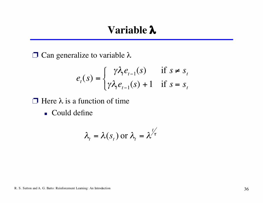
Variable λ

❐ Can generalize to variable λ

❐ Here λ is a function of time Could define

et(s) =

!"tet#1(s) if s $ s

t

!"tet#1(s) +1 if s = s

t

% & '

!""""t

ttts == or )(


Conclusions

❐ Provides efficient, incremental way to combine MC andTD Includes advantages of MC (can deal with lack of

Markov property) Includes advantages of TD (using TD error,

bootstrapping)❐ Can significantly speed learning❐ Does have a cost in computation


Something Here is Not Like the Other

Chapter 7: Eligibility Traces - UMass Amherst

Documents