Chapter 7 Confidence Intervals and Sample Size 1 Copyright © 2012 The McGraw-Hill Companies, Inc. Permission required for reproduction or display.

Chapter 7 Confidence Intervals and Sample Size 1 Copyright © 2012 The McGraw-Hill Companies, Inc. Permission required for reproduction or display.
Dec 19, 2015
Welcome message from author
This document is posted to help you gain knowledge. Please leave a comment to let me know what you think about it! Share it to your friends and learn new things together.
Transcript
Chapter 7
Confidence Intervals and Sample Size
1Copyright © 2012 The McGraw-Hill Companies, Inc. Permission required for reproduction or display.

C H A P T E R
Outline7Confidence Intervals and Sample
Size
1.1Descriptive and Inferential Statistics
Slide 2Copyright © 2012 The McGraw-Hill Companies, Inc.
7-1 Confidence Intervals for the Mean When Is Known
7-2 Confidence Intervals for the Mean When Is Unknown
7-3 Confidence Intervals and Sample Size for Proportions
7-4 Confidence Intervals for Variances and Standard Deviations

C H A P T E R
Objectives7Confidence Intervals and Sample
Size
1.1Descriptive and inferential statistics
1 Find the confidence interval for the mean when is known.
2 Determine the minimum sample size for finding a confidence interval for the mean.
3 Find the confidence interval for the mean when is unknown.
4 Find the confidence interval for a proportion.5 Determine the minimum sample size for finding a
confidence interval for a proportion.

C H A P T E R
Objectives7Confidence Intervals and Sample
Size
1.1Descriptive and inferential statistics
6 Find a confidence interval for a variance and a standard deviation.
7.1 Confidence Intervals for the Mean When Is Known
A point estimate is a specific numerical value estimate of a parameter.
The best point estimate of the population mean µ is the sample mean .X
5Bluman Chapter 7

Three Properties of a Good Estimator
1. The estimator should be an unbiased estimator. That is, the expected value or the mean of the estimates obtained from samples of a given size is equal to the parameter being estimated.
6Bluman Chapter 7

Three Properties of a Good Estimator
2. The estimator should be consistent. For a consistent estimator, as sample size increases, the value of the estimator approaches the value of the parameter estimated.
7Bluman Chapter 7
Three Properties of a Good Estimator
3. The estimator should be a relatively efficient estimator; that is, of all the statistics that can be used to estimate a parameter, the relatively efficient estimator has the smallest variance.
8Bluman Chapter 7

Confidence Intervals for the Mean When Is Known
An interval estimate of a parameter is an interval or a range of values used to estimate the parameter.
This estimate may or may not contain the value of the parameter being estimated.
9Bluman Chapter 7

Confidence Level of an Interval Estimate
The confidence level of an interval estimate of a parameter is the probability that the interval estimate will contain the parameter, assuming that a large number of samples are selected and that the estimation process on the same parameter is repeated.
10Bluman Chapter 7
Confidence Interval
A confidence interval is a specific interval estimate of a parameter determined by using data obtained from a sample and by using the specific confidence level of the estimate.
11Bluman Chapter 7

Formula for the Confidence Interval of the Mean for a Specific a
/ 2 / 2X z X zn n
For a 90% confidence interval: / 2 1.65z
/ 2 1.96z
/ 2 2.58z For a 99% confidence interval:
For a 95% confidence interval:
12Bluman Chapter 7
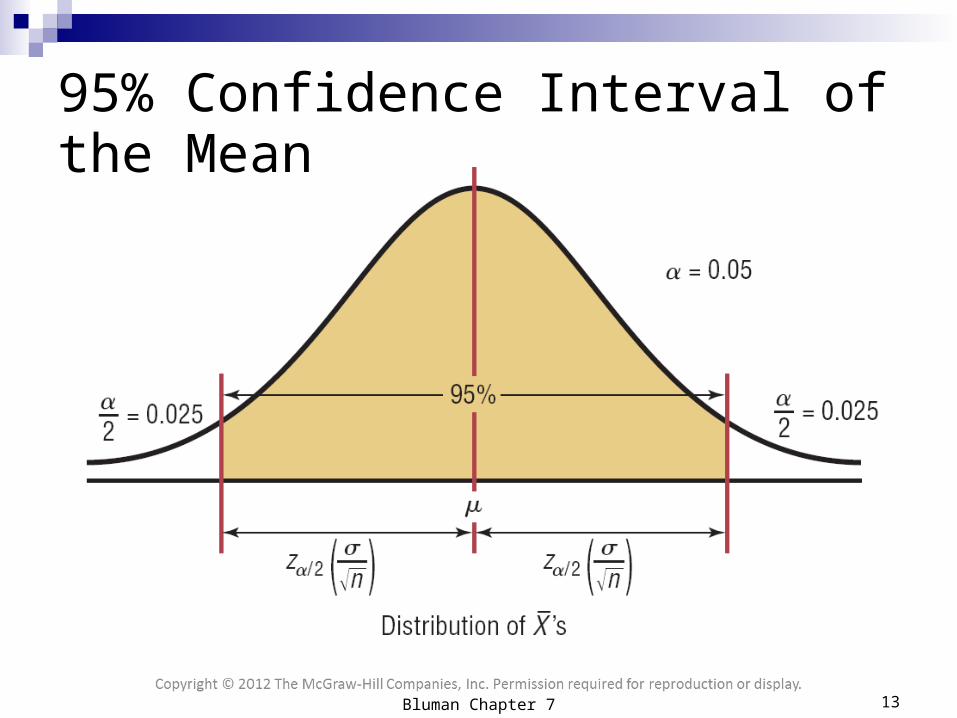
95% Confidence Interval of the Mean
13Bluman Chapter 7

Maximum Error of the Estimate
/ 2E zn
The maximum error of the estimate is the maximum likely difference between the point estimate of a parameter and the actual value of the parameter.
14Bluman Chapter 7
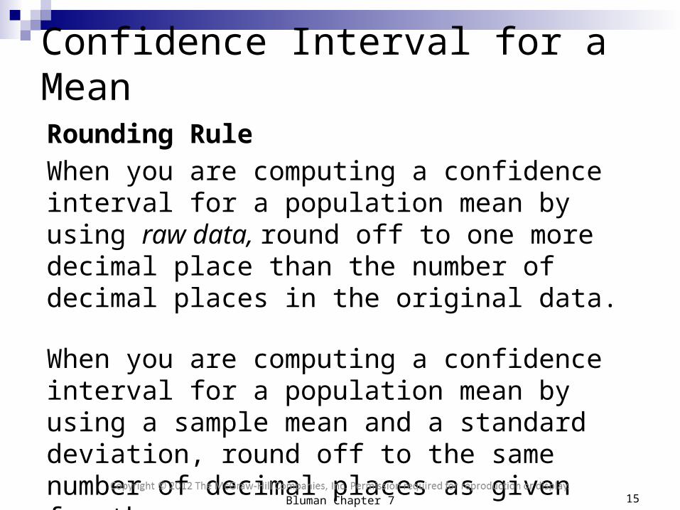
Rounding Rule
When you are computing a confidence interval for a population mean by using raw data, round off to one more decimal place than the number of decimal places in the original data.
When you are computing a confidence interval for a population mean by using a sample mean and a standard deviation, round off to the same number of decimal places as given for the mean.
Confidence Interval for a Mean
15Bluman Chapter 7

Chapter 7Confidence Intervals and Sample Size
Section 7-1Example 7-1
Page #360
16Bluman Chapter 7

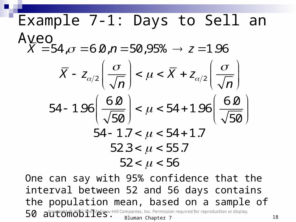
Example 7-1: Days to Sell an AveoA researcher wishes to estimate the number of days it takes an automobile dealer to sell a Chevrolet Aveo. A sample of 50 cars had a mean time on the dealer’s lot of 54 days. Assume the population standard deviation to be 6.0 days. Find the best point estimate of the population mean and the 95% confidence interval of the population mean.
The best point estimate of the mean is 54 days.
54, 6.0, 50,95% 1.96X n z
2 2
X z X zn n
17Bluman Chapter 7
Example 7-1: Days to Sell an Aveo
One can say with 95% confidence that the interval between 52 and 56 days contains the population mean, based on a sample of 50 automobiles.
54, 6.0, 50,95% 1.96X n z
6.0 6.054 1.96 54 1.96
50 50
2 2
X z X zn n
54 1.7 54 1.7 52.3 55.7
52 56
18Bluman Chapter 7

Chapter 7Confidence Intervals and Sample Size
Section 7-1Example 7-2
Page #360
19Bluman Chapter 7
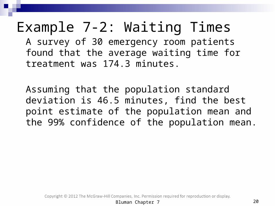
Example 7-2: Waiting TimesA survey of 30 emergency room patients found that the average waiting time for treatment was 174.3 minutes.
Assuming that the population standard deviation is 46.5 minutes, find the best point estimate of the population mean and the 99% confidence of the population mean.
20Bluman Chapter 7
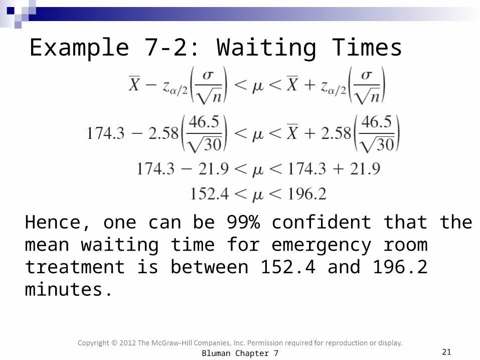
Example 7-2: Waiting Times
Hence, one can be 99% confident that the mean waiting time for emergency room treatment is between 152.4 and 196.2 minutes.
21Bluman Chapter 7

95% Confidence Interval of the Mean
22Bluman Chapter 7
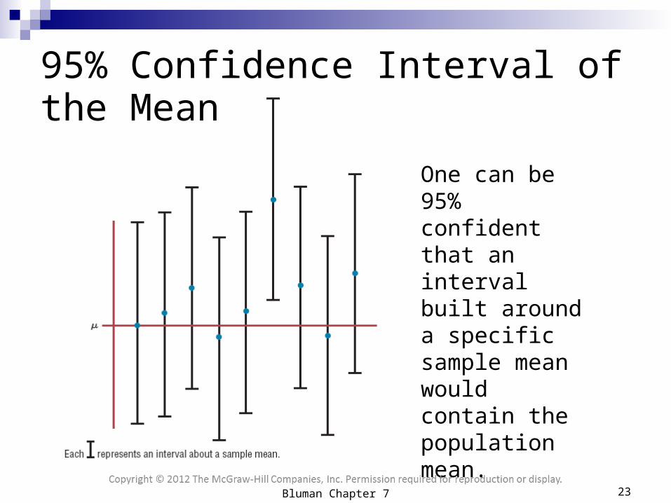
95% Confidence Interval of the Mean
One can be 95% confident that an interval built around a specific sample mean would contain the population mean.
23Bluman Chapter 7

Finding for 98% CL.2z
2 2.33z
24Bluman Chapter 7

Chapter 7Confidence Intervals and Sample Size
Section 7-1Example 7-3
Page #362
25Bluman Chapter 7

Example 7-3: Credit Union AssetsThe following data represent a sample of the assets (in millions of dollars) of 30 credit unions in southwestern Pennsylvania. Find the 90% confidence interval of the mean.
12.23 16.56 4.39 2.89 1.24 2.1713.19 9.16 1.4273.25 1.91 14.6411.59 6.69 1.06 8.74 3.17 18.13 7.92 4.78 16.8540.22 2.42 21.58 5.01 1.47 12.24 2.27 12.77 2.76
26Bluman Chapter 7
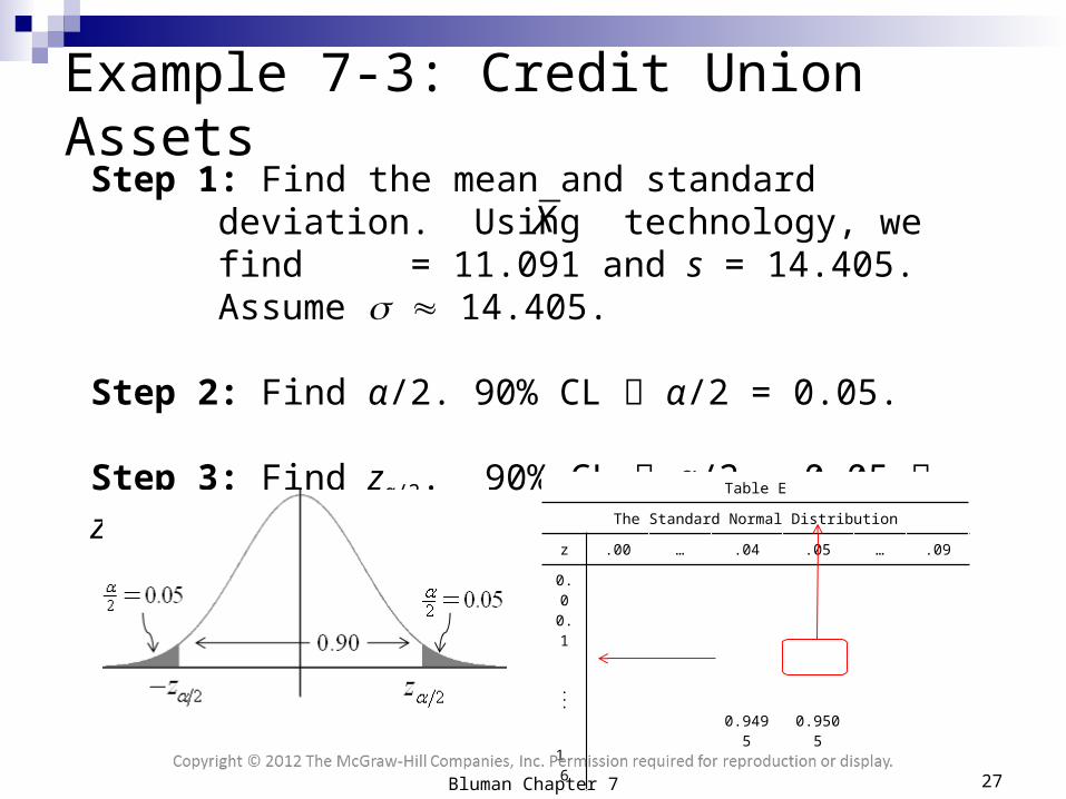
Example 7-3: Credit Union AssetsStep 1: Find the mean and standard deviation. Using
technology, we find = 11.091 and s = 14.405. Assume 14.405.
Step 2: Find α/2. 90% CL α/2 = 0.05.
Step 3: Find zα/2. 90% CL α/2 = 0.05 z.05 = 1.65
X
Table E
The Standard Normal Distribution
z .00 … .04 .05 … .09
0.00.1
...
1.6 0.9495 0.9505
27Bluman Chapter 7

Example 7-3: Credit Union AssetsStep 4: Substitute in the formula.
One can be 90% confident that the population mean of the assets of all credit unions is between $6.752 million and $15.430 million, based on a sample of 30 credit unions.
14.405 14.40511.091 1.65 11.091 1.65
30 30
2 2
X z X zn n
11.091 4.339 11.091 4.339 6.752 15.430
28Bluman Chapter 7

This chapter and subsequent chapters include examples using raw data. If you are using computer or calculator programs to find the solutions, the answers you get may vary somewhat from the ones given in the textbook.
This is so because computers and calculators do not round the answers in the intermediate steps and can use 12 or more decimal places for computation. Also, they use more exact values than those given in the tables in the back of this book.
These discrepancies are part and parcel of statistics.
Technology Note
29Bluman Chapter 7
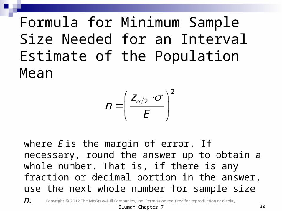
where E is the margin of error. If necessary, round the answer up to obtain a whole number. That is, if there is any fraction or decimal portion in the answer, use the next whole number for sample size n.
Formula for Minimum Sample Size Needed for an Interval Estimate of the Population Mean
2
2
zn
E
30Bluman Chapter 7

Chapter 7Confidence Intervals and Sample Size
Section 7-1Example 7-4
Page #364
31Bluman Chapter 7

Example 7-4: Depth of a RiverA scientist wishes to estimate the average depth of a river. He wants to be 99% confident that the estimate is accurate within 2 feet. From a previous study, the standard deviation of the depths measured was 4.33 feet. How large a sample is required?
Therefore, to be 99% confident that the estimate is within 2 feet of the true mean depth, the scientist needs at least a sample of 32 measurements.
99% 2.58, 2, 4.33z E 2
2
zn
E 2
2.58 4.33
2
31.2 32
32Bluman Chapter 7

7.2 Confidence Intervals for the Mean When Is Unknown
The value of , when it is not known, must be estimated by using s, the standard deviation of the sample.
When s is used, especially when the sample size is small (less than 30), critical values greater than the values for are used in confidence intervals in order to keep the interval at a given level, such as the 95%.
These values are taken from the Student t distribution, most often called the t distribution.
2z
33Bluman Chapter 7

Characteristics of the t DistributionThe t distribution is similar to the standard normal distribution in these ways:
1. It is bell-shaped.
2. It is symmetric about the mean.
3. The mean, median, and mode are equal to 0 and are located at the center of the distribution.
4. The curve never touches the x axis.
34Bluman Chapter 7

Characteristics of the t DistributionThe t distribution differs from the standard normal distribution in the following ways:
1. The variance is greater than 1.
2. The t distribution is actually a family of curves based on the concept of degrees of freedom, which is related to sample size.
3. As the sample size increases, the t distribution approaches the standard normal distribution.
35Bluman Chapter 7
Degrees of Freedom The symbol d.f. will be used for degrees of
freedom. The degrees of freedom for a confidence
interval for the mean are found by subtracting 1 from the sample size. That is, d.f. = n – 1.
Note: For some statistical tests used later in this book, the degrees of freedom are not equal to n – 1.
36Bluman Chapter 7

The degrees of freedom are n – 1.
Formula for a Specific Confidence Interval for the Mean When IsUnknown and n < 30
2 2
s sX t X t
n n
37Bluman Chapter 7

Chapter 7Confidence Intervals and Sample Size
Section 7-2Example 7-5
Page #371
38Bluman Chapter 7
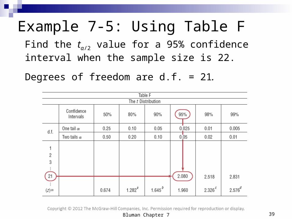
Find the tα/2 value for a 95% confidence interval when the sample size is 22.
Degrees of freedom are d.f. = 21.
Example 7-5: Using Table F
39Bluman Chapter 7

Chapter 7Confidence Intervals and Sample Size
Section 7-2Example 7-6
Page #372
40Bluman Chapter 7

Ten randomly selected people were asked how long they slept at night. The mean time was 7.1 hours, and the standard deviation was 0.78 hour. Find the 95% confidence interval of the mean time. Assume the variable is normally distributed.
Since is unknown and s must replace it, the t distribution (Table F) must be used for the confidence interval. Hence, with 9 degrees of freedom, tα/2 = 2.262.
Example 7-6: Sleeping Time
2 2
s sX t X t
n n
0.78 0.787.1 2.262 7.1 2.262
10 10
41Bluman Chapter 7

One can be 95% confident that the population mean is between 6.5 and 7.7 hours.
Example 7-6: Sleeping Time
0.78 0.787.1 2.262 7.1 2.262
10 10
7.1 0.56 7.1 0.56
6.5 7.7
42Bluman Chapter 7

Chapter 7Confidence Intervals and Sample Size
Section 7-2Example 7-7
Page #372
43Bluman Chapter 7
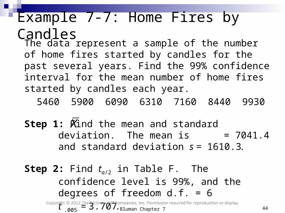
The data represent a sample of the number of home fires started by candles for the past several years. Find the 99% confidence interval for the mean number of home fires started by candles each year.
5460 5900 6090 6310 7160 8440 9930
Step 1: Find the mean and standard deviation. The mean is = 7041.4 and standard deviation s = 1610.3.
Step 2: Find tα/2 in Table F. The confidence level is 99%, and the degrees of freedom d.f. = 6
t .005 = 3.707.
Example 7-7: Home Fires by Candles
X
44Bluman Chapter 7
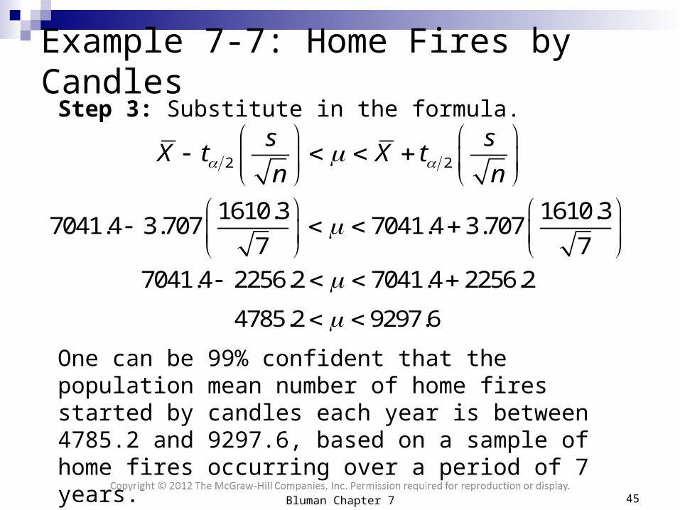
Example 7-7: Home Fires by CandlesStep 3: Substitute in the formula.
One can be 99% confident that the population mean number of home fires started by candles each year is between 4785.2 and 9297.6, based on a sample of home fires occurring over a period of 7 years.
1610.3 1610.37041.4 3.707 7041.4 3.707
7 7
2 2
s sX t X t
n n
7041.4 2256.2 7041.4 2256.2
4785.2 9297.6
45Bluman Chapter 7
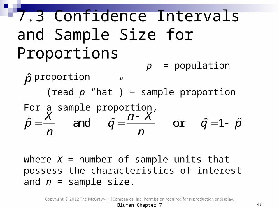
7.3 Confidence Intervals and Sample Size for Proportions
p = population proportion
(read p “hat”) = sample proportion
For a sample proportion,
where X = number of sample units that possess the characteristics of interest and n = sample size.
p̂
ˆ ˆ ˆ ˆand or 1X n X
p q q pn n
46Bluman Chapter 7

Chapter 7Confidence Intervals and Sample Size
Section 7-3Example 7-8
Page #378
47Bluman Chapter 7

In a recent survey of 150 households, 54 had central air conditioning. Find and , where is the proportion of households that have central air conditioning.
Since X = 54 and n = 150,
Example 7-8: Air Conditioned Households
54ˆ 0.36 36%
150
Xp
n
ˆ ˆ1 1 0.36 0.64 64% q p
p̂ q̂ p̂
48Bluman Chapter 7

when np 5 and nq 5.
Formula for a Specific Confidence Interval for a Proportion
2 2
ˆ ˆ ˆ ˆˆ ˆ
pq pqp z p p z
n n
Rounding Rule: Round off to three decimal places.
49Bluman Chapter 7
Chapter 7Confidence Intervals and Sample Size
Section 7-3Example 7-9
Page #379
50Bluman Chapter 7

A survey conducted by Sallie Mae and Gallup of 1404 respondents found that 323 students paid for their education by student loans.
Find the 90% confidence of the true proportion of students who paid for their education by student loans.
Example 7-9: Covering College Costs
51Bluman Chapter 7
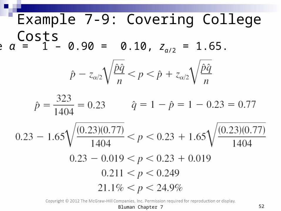
Example 7-9: Covering College CostsSince α = 1 – 0.90 = 0.10, zα/2 = 1.65.
52Bluman Chapter 7

Example 7-9: Covering College CostsYou can be 90% confident that the percentage of students who pay for their college education by student loans is between 21.1 and 24.9%.
53Bluman Chapter 7

Chapter 7Confidence Intervals and Sample Size
Section 7-3Example 7-10
Page #379
54Bluman Chapter 7

A survey of 1721 people found that 15.9% of individuals purchase religious books at a Christian bookstore. Find the 95% confidence interval of the true proportion of people who purchase their religious books at a Christian bookstore.
Example 7-10: Religious Books
0.159 0.841 0.159 0.8410.159 1.96 0.159 1.96
1721 1721 p
0.142 0.176 p
You can say with 95% confidence that the true percentage is between 14.2% and 17.6%.
2 2
ˆ ˆ ˆ ˆˆ ˆ
pq pqp z p p z
n n
55Bluman Chapter 7

If necessary, round up to the next whole number.
Formula for Minimum Sample Size Needed for Interval Estimate of a Population Proportion
2
2ˆ ˆ
zn pq
E
56Bluman Chapter 7
Chapter 7Confidence Intervals and Sample Size
Section 7-3Example 7-11
Page #380
57Bluman Chapter 7

A researcher wishes to estimate, with 95% confidence, the proportion of people who own a home computer. A previous study shows that 40% of those interviewed had a computer at home. The researcher wishes to be accurate within 2% of the true proportion. Find the minimum sample size necessary.
Example 7-11: Home Computers
2
1.960.40 0.60
0.02
2304.96
The researcher should interview a sample of at least 2305 people.
2
2ˆ ˆ
zn pq
E
58Bluman Chapter 7

Chapter 7Confidence Intervals and Sample Size
Section 7-3Example 7-12
Page #380
59Bluman Chapter 7
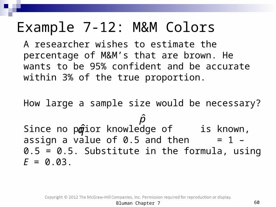
A researcher wishes to estimate the percentage of M&M’s that are brown. He wants to be 95% confident and be accurate within 3% of the true proportion.
How large a sample size would be necessary?
Since no prior knowledge of is known, assign a value of 0.5 and then = 1 – 0.5 = 0.5. Substitute in the formula, using E = 0.03.
Example 7-12: M&M Colors
p̂q̂
60Bluman Chapter 7
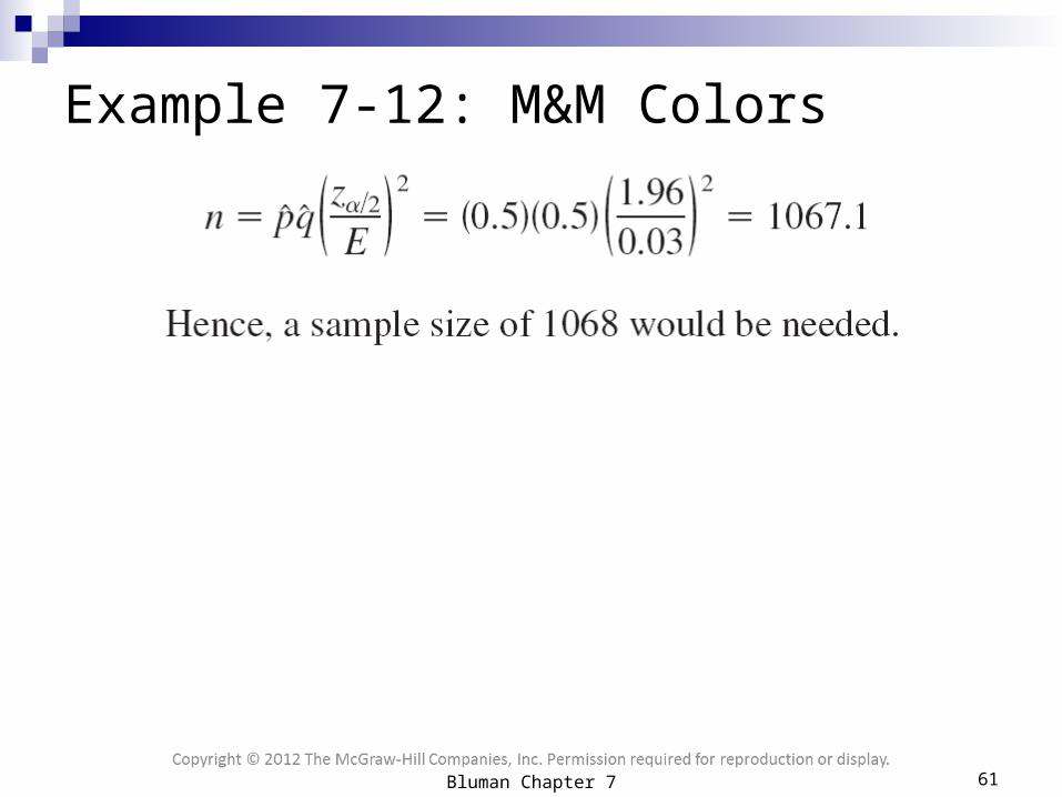
Example 7-12: M&M Colors
61Bluman Chapter 7
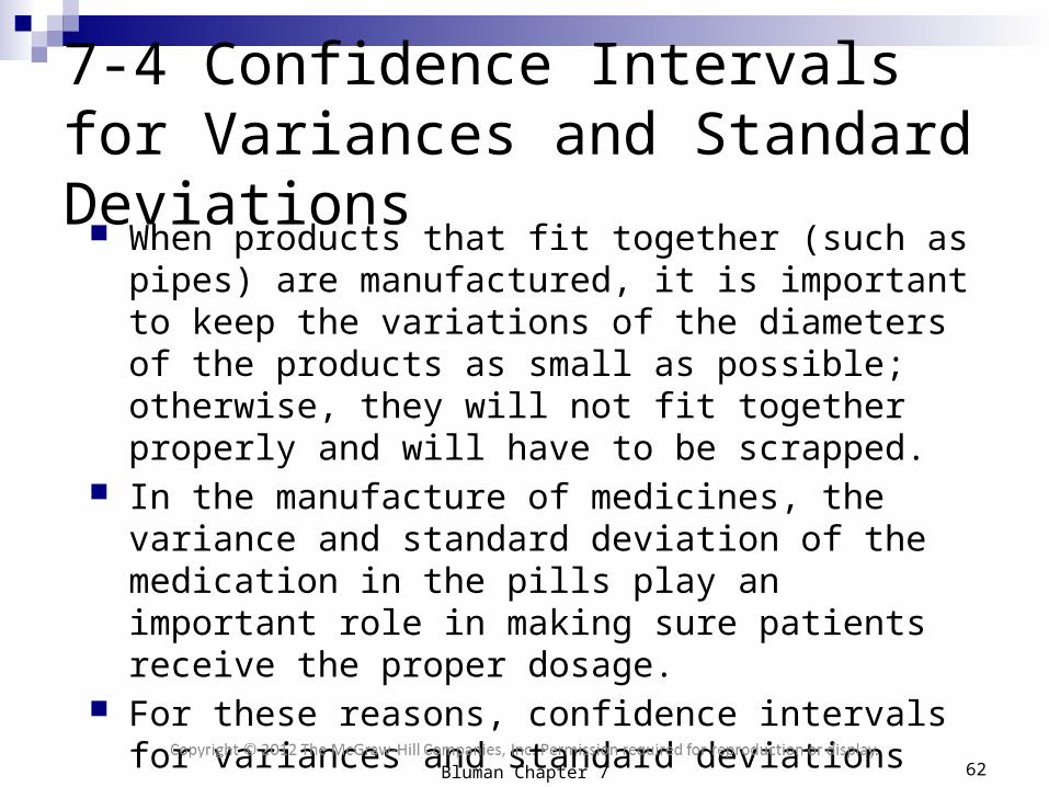
7-4 Confidence Intervals for Variances and Standard Deviations
When products that fit together (such as pipes) are manufactured, it is important to keep the variations of the diameters of the products as small as possible; otherwise, they will not fit together properly and will have to be scrapped.
In the manufacture of medicines, the variance and standard deviation of the medication in the pills play an important role in making sure patients receive the proper dosage.
For these reasons, confidence intervals for variances and standard deviations are necessary.
62Bluman Chapter 7

Chi-Square Distributions The chi-square distribution must be used to calculate
confidence intervals for variances and standard deviations.
The chi-square variable is similar to the t variable in that its distribution is a family of curves based on the number of degrees of freedom.
The symbol for chi-square is (Greek letter chi, pronounced “ki”).
A chi-square variable cannot be negative, and the distributions are skewed to the right.
2
63Bluman Chapter 7

Chi-Square Distributions At about 100 degrees of freedom, the chi-square
distribution becomes somewhat symmetric.
The area under each chi-square distribution is equal to 1.00, or 100%.
64Bluman Chapter 7

Formula for the Confidence Interval for a Variance
2 22
2 2right left
1 1, d.f. = 1
n s n sn
Formula for the Confidence Interval for a Standard Deviation
2 2
2 2right left
1 1, d.f. = 1
n s n sn
65Bluman Chapter 7

Chapter 7Confidence Intervals and Sample Size
Section 7-4Example 7-13
Page #387
66Bluman Chapter 7

Find the values for and for a 90% confidence interval when n = 25.
Example 7-13: Using Table G
To find , subtract 1 – 0.90 = 0.10. Divide by 2 to get 0.05.To find , subtract 1 – 0.05 to get 0.95.
2left2
right
2right2left
67Bluman Chapter 7
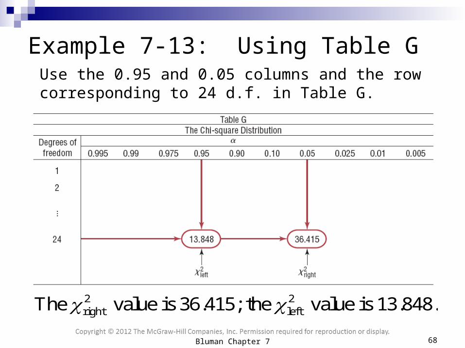
Use the 0.95 and 0.05 columns and the row corresponding to 24 d.f. in Table G.
Example 7-13: Using Table G
2 2right leftThe value is 36.415; the value is 13.848.
68Bluman Chapter 7

Rounding Rule
When you are computing a confidence interval for a population variance or standard deviation by using raw data, round off to one more decimal places than the number of decimal places in the original data.
When you are computing a confidence interval for a population variance or standard deviation by using a sample variance or standard deviation, round off to the same number of decimal places as given for the sample variance or standard deviation.
Confidence Interval for a Variance or Standard Deviation
69Bluman Chapter 7
Chapter 7Confidence Intervals and Sample Size
Section 7-4Example 7-14
Page #389
70Bluman Chapter 7

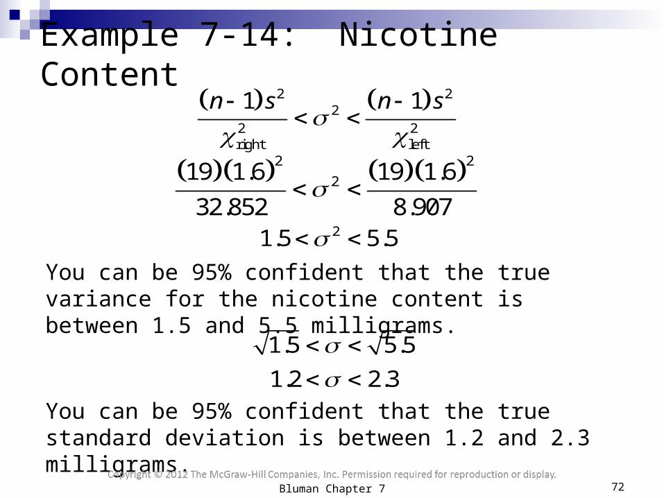
Find the 95% confidence interval for the variance and standard deviation of the nicotine content of cigarettes manufactured if a sample of 20 cigarettes has a standard deviation of 1.6 milligrams.
Example 7-14: Nicotine Content
To find , subtract 1 – 0.95 = 0.05. Divide by 2 to get 0.025.
To find , subtract 1 – 0.025 to get 0.975.
In Table G, the 0.025 and 0.975 columns with the d.f. 19 row yield values of 32.852 and 8.907, respectively.
2right
2left
71Bluman Chapter 7
Example 7-14: Nicotine Content 2 2
22 2right left
1 1
n s n s
21.5 5.5
1.5 5.5
1.2 2.3
You can be 95% confident that the true variance for the nicotine content is between 1.5 and 5.5 milligrams.
2 2
219 1.6 19 1.6
32.852 8.907
You can be 95% confident that the true standard deviation is between 1.2 and 2.3 milligrams.
72Bluman Chapter 7

Chapter 7Confidence Intervals and Sample Size
Section 7-4Example 7-15
Page #389
73Bluman Chapter 7
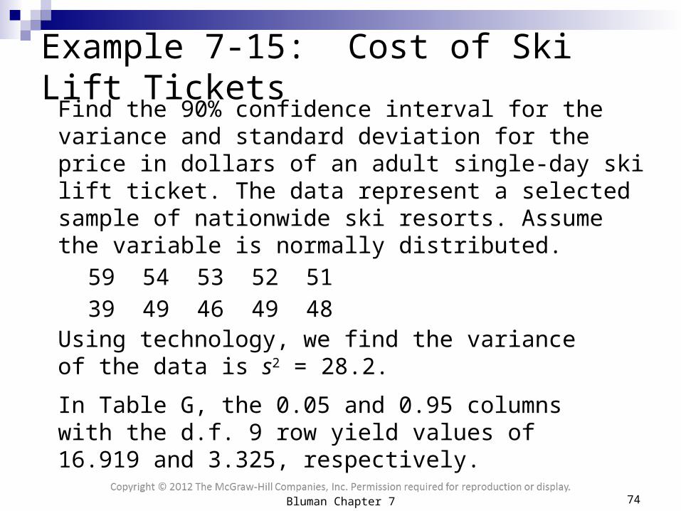
Find the 90% confidence interval for the variance and standard deviation for the price in dollars of an adult single-day ski lift ticket. The data represent a selected sample of nationwide ski resorts. Assume the variable is normally distributed.
59 54 53 52 51
39 49 46 49 48
Example 7-15: Cost of Ski Lift Tickets
Using technology, we find the variance of the data is s2 = 28.2.
In Table G, the 0.05 and 0.95 columns with the d.f. 9 row yield values of 16.919 and 3.325, respectively.
74Bluman Chapter 7

Example 7-15: Cost of Ski Lift Tickets 2 2
22 2right left
1 1
n s n s
215.0 76.3
15.0 76.3
3.87 8.73
You can be 95% confident that the true variance for the cost of ski lift tickets is between 15.0 and 76.3.
29 28.2 9 28.2
16.919 3.325
You can be 95% confident that the true standard deviation is between $3.87 and $8.73.
75Bluman Chapter 7
Related Documents