Chapter 7: Choosing Functional Forms

Chapter 7: Choosing Functional Forms

1. The World Is Not Flat Things would be relatively simple if we could always presume that our first simplifying assumption in

Chapter Five is true. If all population relationships were linear, all regressions could take the form we have

been studying. But at the heart of economics is the knowledge that linearity is often a poor approximation

of the truth. We experience diminishing, not constant, marginal utility; firms experience diminishing

marginal returns, and average cost curves are therefore convex; elasticities of demand and supply usually

change as prices change; inflation accelerates as unemployment rates fall.

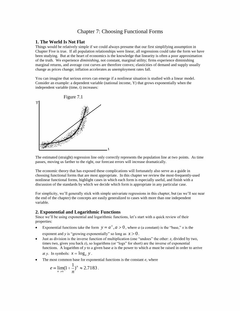
You can imagine that serious errors can emerge if a nonlinear situation is studied with a linear model.

Consider an example: a dependent variable (national income, Y) that grows exponentially when the

independent variable (time, t) increases:

Figure 7.1

The estimated (straight) regression line only correctly represents the population line at two points. As time

passes, moving us farther to the right, our forecast errors will increase dramatically.

The economic theory that has exposed these complications will fortunately also serve as a guide in

choosing functional forms that are most appropriate. In this chapter we review the most-frequently-used

nonlinear functional forms, highlight cases in which each form is especially useful, and finish with a

discussion of the standards by which we decide which form is appropriate in any particular case.

For simplicity, we’ll generally stick with simple univariate regressions in this chapter, but (as we’ll see near

the end of the chapter) the concepts are easily generalized to cases with more than one independent

variable.

2. Exponential and Logarithmic Functions Since we’ll be using exponential and logarithmic functions, let’s start with a quick review of their

properties:

Exponential functions take the form 0, aay x, where a (a constant) is the “base,” x is the

exponent and y is “growing exponentially” so long as 0x .

Just as division is the inverse function of multiplication (one “undoes” the other: z, divided by two,

times two, gives you back z), so logarithms (or “logs” for short) are the inverse of exponential

functions. A logarithm of y to a given base a is the power to which a must be raised in order to arrive

at y. In symbols: yx alog .

The most common base for exponential functions is the constant e, where

7183.2)1

1(lim n

n ne .

Thus the most common logarithms are logs to the base e, which are so common that we just call them

“natural logs” and simplify the notation from yx elog to yx ln (pronounced “x is the natural

log of y,” not “x is elllnn-y.”). In pictures:

Figure 7.2 Figure 7.3

Why has such an uncommon pair of things become so common? Remember that we are looking for some

clever transformations of variables that will have some desirable properties. These two functions happen to

have some attributes that will prove to be very useful:

Both exponential and logarithmic functions are monotonic increasing transformations. If we have two

numbers i and k where ki , then ki ee and )ln()ln( ki .

Log operations: for any two positive numbers c and k ,

)ln()ln()ln( kckc [“log of product is sum of logs”] 7.1

)ln()ln(ln kck

c, [which implies that )ln(

1ln k

k] 7.2

)ln()ln( ckc k [looks like the power rule in calculus, no?] 7.3

Exponential Function operations:

)ln(ckk ec [implied by 7.3] 7.4

kckc aaa 7.5

)()( kckc aa 7.6

We introduced these functions because we want to allow for nonlinear relationships among variables—we

want to allow the derivative of Y with respect to X to not be a constant, but rather to vary as X changes.

Let’s review the properties of the derivatives of logarithmic and exponential functions:

If )ln(XY , then XdX

dY 1. 7.7

If XeY , then

XedX

dY as well. 7.8

If XaeY , then

XaeadX

dY 7.9

If XaY , then )ln(aa

dX

dY X 7.10

Finally, elasticities are sometimes important in economics, so we should identify the elasticity of Y with

respect to X for exponential and logarithmic functions:

By definition, let Y

X

dX

dY

X

Y

%

%. Then the properties we’ve just listed imply:

If )ln(XaY , then Y

a. 7.11

If XeY , then X

e

Xe

Y

Xe

X

XX 7.12

Having reviewed the properties of logarithmic and exponential functions, it’s time to study the most

common transformations by which models are made to appear linear, so that OLS estimation can proceed.

We’ll study nine common transformations, and the first three involve logs and exponential functions.

3. The Linear-Log, Log-Linear, and Log-Log Forms These three options all involve the natural logarithm of at least one variable:

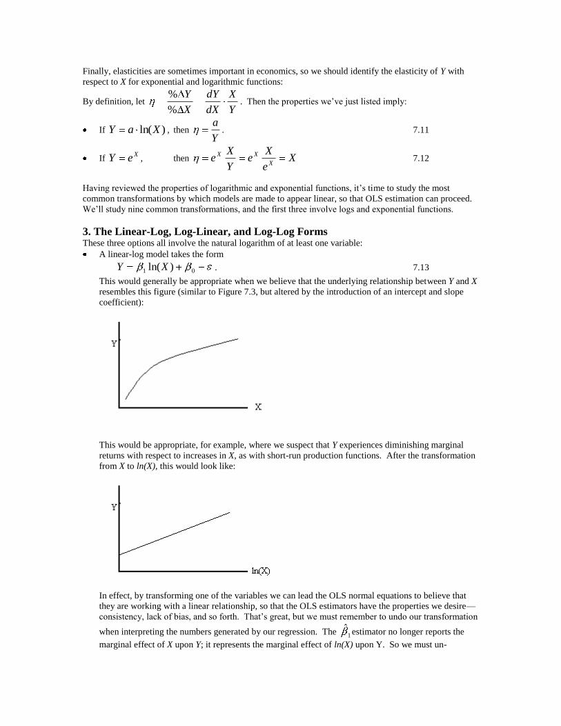
A linear-log model takes the form

01 )ln(XY . 7.13

This would generally be appropriate when we believe that the underlying relationship between Y and X

resembles this figure (similar to Figure 7.3, but altered by the introduction of an intercept and slope

coefficient):

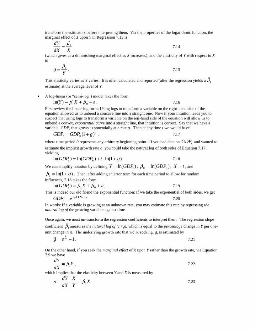
This would be appropriate, for example, where we suspect that Y experiences diminishing marginal

returns with respect to increases in X, as with short-run production functions. After the transformation

from X to ln(X), this would look like:

In effect, by transforming one of the variables we can lead the OLS normal equations to believe that

they are working with a linear relationship, so that the OLS estimators have the properties we desire—

consistency, lack of bias, and so forth. That’s great, but we must remember to undo our transformation

when interpreting the numbers generated by our regression. The 1ˆ estimator no longer reports the

marginal effect of X upon Y; it represents the marginal effect of ln(X) upon Y. So we must un-

transform the estimators before interpreting them. Via the properties of the logarithmic function, the

marginal effect of X upon Y in Regression 7.13 is

XdX

dY 1 7.14

(which gives us a diminishing marginal effect as X increases), and the elasticity of Y with respect to X

is

Y

1. 7.15

This elasticity varies as Y varies. It is often calculated and reported (after the regression yields a1

ˆ

estimate) at the average level of Y.

A log-linear (or “semi-log”) model takes the form

01)ln( XY . 7.16

First review the linear-log form: Using logs to transform a variable on the right-hand side of the

equation allowed us to unbend a concave line into a straight one. Now if your intuition leads you to

suspect that using logs to transform a variable on the left-hand side of the equation will allow us to

unbend a convex, exponential curve into a straight line, that intuition is correct. Say that we have a

variable, GDP, that grows exponentially at a rate g. Then at any time t we would have t

t gGDPGDP )1(0 , 7.17

where time period 0 represents any arbitrary beginning point. If you had data on tGDP and wanted to

estimate the implicit growth rate g, you could take the natural log of both sides of Equation 7.17,

yielding

)1ln()ln()ln( 0 gtGDPGDPt 7.18

We can simplify notation by defining )ln( tGDPY , )ln( 00 GDP , tX , and

)1ln(1 g . Then, after adding an error term for each time period to allow for random

influences, 7.18 takes the form

tt XGDP 01)ln( 7.19

This is indeed our old friend the exponential function: If we take the exponential of both sides, we get

tX

t eGDP 01 7.20

In words: If a variable is growing at an unknown rate, you may estimate this rate by regressing the

natural log of the growing variable against time.

Once again, we must un-transform the regression coefficients to interpret them. The regression slope

coefficient 1ˆ measures the natural log of (1+g), which is equal to the percentage change in Y per one-

unit change in X. The underlying growth rate that we’re seeking, g, is estimated by

1ˆ 1ˆ

eg . 7.21

On the other hand, if you seek the marginal effect of X upon Y rather than the growth rate, via Equation

7.9 we have

YdX

dY1 , 7.22

which implies that the elasticity between Y and X is measured by

XY

X

dX

dY1 7.23

There’s one more twist: Say that you want to use our regression to make forecasts of y by inserting

some expected value of x into the regression equation. If you take the expected value of 7.20, you’ll

have

)(()( 0101 ) tt eEeeEGDPEtt

t , 7.24

which would be fine if )( teE were equal to one. Then the forecast would be unbiased, consistent

and efficient. Unfortunately,

1)( 2

2

eeE t , 7.25

so we must correct for this bias by using the following equation to forecast the dependent variable in

log-linear regressions:

)2

ˆ(ˆˆ 2

01ˆ tx

t ey , 7.26

where 2ˆ is the sample variance of the error terms.

A log-log (or “double-log”)model takes the form

01 )ln()ln( XY . 7.27

This form is very popular for estimating production and demand functions, because of some

convenient properties of the estimates. Let’s allow a multivariate regression for a moment, to point out

some of these properties.

Imagine that a process producing Q uses two inputs, L and K, and is also subject to changes in

technology measured by a parameter a. If the production function happened to take the form

aLKQ 21 , 7.28

we could take the log of both sides, add an error term, and arrive at

021 )ln()ln()ln( LKQ , 7.29

where we’ve simplified by defining )ln(0 a . This would be easy to estimate, and the coefficients

happen to have lovely properties:

The kˆ are unbiased estimators of the elasticity of Q with respect to the independent variables,

and the sum of the kˆ estimates gives us a measure of returns to scale: If they sum to a number greater

than one there are increasing returns. A sum less than one indicates decreasing returns, and

coefficients summing to one signifies constant returns.

We can also derive the marginal effect of X upon Y in this form:

k

kx

y

dx

dy. 7.30

You may suspect that the tail of convenience is wagging the theoretical dog in this case. We get easy-

to-calculate elasticity estimates, but get them by assuming that the elasticities are constants. In our

economic theory courses we were led to believe that elasticities often vary along demand curves and

production functions. Before the chapter is over we will discuss ways of testing the relevance of this

form for any particular situation. For now we can say that this form was popularized several

generations ago by the work of Cobb and Douglas, who argued that this log-log form fit production-

unction data better than the competitors. For that reason the log-log form is often called the “Cobb-

Douglas function.”

4. Polynomial and Reciprocal Forms

We began modeling nonlinear relationships with the rather exotic logarithmic and exponential functions.

You may have been more familiar with the polynomial forms, which are simple extensions of the linear

form: To the regression equation

01xy

we can add polynomial terms that allow the relationship between X and Y to be nonlinear:

0

2

21

k

k xxxy

Adding just a squared term (a quadratic equation, or polynomial of degree two) allows relationships that

resemble the following possibilities:

0,0, 120

0,, 210

Adding both a squared and cubed term (a cubic function) allows amplified versions of these last two

graphs, when the coefficient on the cubed term has the same sign as that of the squared term and linear

term. Cubic terms also allow points of inflection, when the linear and squared term have the opposite sign

of the cubed term:

0,0,, 3210

The quadratic form is sometimes used to fit short-run cost data, as it allows the characteristic U-shape we’d

want to allow. The cubic function is sometimes used to fit short-run production functions, where we want to

allow the possibility of returns to a fixed factor that at first increase, then decrease.

The derivatives and elasticities of polynomial functions are easy to find, using the properties of derivatives.

For example, the derivative of y with respect to x in the quadratic form is x21 2 , and the elasticity of

y is equal to y

xx

y

x

dx

dy)2( 21

.

Polynomials of degrees greater than three are possible, but usually frowned upon. The extra terms burn up

degrees of freedom, and as we will see in the next chapter, lead to a problem called multicollinearity, usually

without much of an offsetting improvement in explanatory power.

One special case of polynomial regression involves a negative exponent on the independent variable.

Consider the function

010

1

1

1

xxy . 7.31

This “reciprocal” function is sometimes used to estimate demand curves. It has the interesting properties

that y approaches infinity as x shrinks, and approaches the constant 0 as x grows:

0, 01

The marginal effect of x upon y, by the properties of derivatives, is

2

1

xdx

dy, 7.32

and y’s elasticity with respect to x is therefore

yx

1. 7.33

5. Forms with Interaction Terms Consider a new way in which the effect of an independent variable upon y might be nonlinear: What if one

independent variable’s effect upon y depends upon the level of a different independent variable?

For example, consider a demand function in which quantity demanded is influenced by price and income:

021 YPQ 7.34

So far that looks like a simple linear function. But add a twist: Allow the effect of price changes upon

quantity demanded (measured by 1 ) to be influenced by the income of consumers: Lower-income

consumers may be more sensitive to price changes than higher-income consumers. Assuming that this

relationship is also a simple linear one, we can state it in symbols:

011 Y , 7.35

which would look something like a fender from a Stealth Bomber:

In that case we’d have an interaction between the two independent variables. Substitution 7.35 into 7.34

yields

0201 )( YPYQ

or, simplifying terms,

032

'

1 PYYPQ 7.36

This form allows the derivative of q with respect to p to depend on the level of y, as we wished. Note that

the coefficient on p has a new (primed) notation, to signify that it has been “purified” into a true derivative

of q with respect to p while holding y constant.

To do such a regression, we’d create a new variable, equal to the product of the two interacting variables,

then include this new variable with the others in the regression. Note that any regression parameter can be

allowed to depend on other regression variables in this way, and that the interaction can be made more

complicated than the linear interaction of our example.

6. Forms with Lagged Independent Variables: Dynamic Models Imagine that X affects Y with some instantaneous effect, plus an effect that appears after time has passed, or

that Y is influenced by it’s own past values—an inertia effect. Since equilibria don’t emerge immediately

after a change, we’d expect this to be a common occurrence.

A full discussion of dynamic models is beyond the scope of this chapter, but let’s consider a common form

or two in order to introduce several issues we’ll consider in later chapters.

Imagine that you have time-series data (which is what you’d need to estimate a dynamic model). We’ll

date each observation with a subscript t indicating the time period in which it was observed. If you imagine

your matrix of data, the columns would still be individual variables, but the rows would represent different

dates instead of different individuals observed at a single time.

Now consider two straightforward forms for modeling dynamic adjustments of a dependent variable:

We could make the current observation of the dependent variable a function of previous changes in

independent variables—for example, a measure of money supply that responds to changes in reserve

requirements and discount rates, but only after time has passed for the money-expansion multiplier to

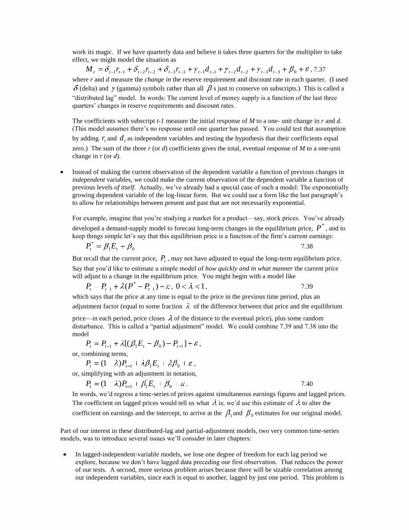
work its magic. If we have quarterly data and believe it takes three quarters for the multiplier to take

effect, we might model the situation as

0332211332211 ttttttttttttt dddrrrM , 7.37

where r and d measure the change in the reserve requirement and discount rate in each quarter. (I used

(delta) and (gamma) symbols rather than all s just to conserve on subscripts.) This is called a

“distributed lag” model. In words: The current level of money supply is a function of the last three

quarters’ changes in reserve requirements and discount rates.

The coefficients with subscript t-1 measure the initial response of M to a one- unit change in r and d.

(This model assumes there’s no response until one quarter has passed. You could test that assumption

by adding tr and td as independent variables and testing the hypothesis that their coefficients equal

zero.) The sum of the three r (or d) coefficients gives the total, eventual response of M to a one-unit

change in r (or d).

Instead of making the current observation of the dependent variable a function of previous changes in

independent variables, we could make the current observation of the dependent variable a function of

previous levels of itself. Actually, we’ve already had a special case of such a model: The exponentially

growing dependent variable of the log-linear form. But we could use a form like the last paragraph’s

to allow for relationships between present and past that are not necessarily exponential.

For example, imagine that you’re studying a market for a product—say, stock prices. You’ve already

developed a demand-supply model to forecast long-term changes in the equilibrium price, *P , and to

keep things simple let’s say that this equilibrium price is a function of the firm’s current earnings:

01

*

tt EP 7.38

But recall that the current price, tP , may not have adjusted to equal the long-term equilibrium price.

Say that you’d like to estimate a simple model of how quickly and in what manner the current price

will adjust to a change in the equilibrium price. You might begin with a model like

)( 1

*

1 ttt PPPP , 10 , 7.39

which says that the price at any time is equal to the price in the previous time period, plus an

adjustment factor (equal to some fraction of the difference between that price and the equilibrium

price—in each period, price closes of the distance to the eventual price), plus some random

disturbance. This is called a “partial adjustment” model. We could combine 7.39 and 7.38 into the

model

])[( 1011 tttt PEPP ,

or, combining terms,

011)1( ttt EPP ,

or, simplifying with an adjustment in notation, '

0

'

11)1( ttt EPP . 7.40

In words, we’d regress a time-series of prices against simultaneous earnings figures and lagged prices.

The coefficient on lagged prices would tell us what is; we’d use this estimate of to alter the

coefficient on earnings and the intercept, to arrive at the 1 and 0 estimates for our original model.

Part of our interest in these distributed-lag and partial-adjustment models, two very common time-series

models, was to introduce several issues we’ll consider in later chapters:

In lagged-independent-variable models, we lose one degree of freedom for each lag period we

explore, because we don’t have lagged data preceding our first observation. That reduces the power

of our tests. A second, more serious problem arises because there will be sizable correlation among

our independent variables, since each is equal to another, lagged by just one period. This problem is

called “multicollinearity,” and its diagnosis, effects and treatment are considered in the next chapter.

The problem is sometimes treated by imposing an assumption about the relative sizes of the

regression coefficients, so that only one must be estimated.

In lagged-dependent-variable models, the OLS estimators are no longer unbiased, and the bias

follows an unpredictable pattern. That’s because each observation of the independent variable is

correlated with the error term of the previous period’s observation, and the bias can be sizable. In

some cases, the estimators are still consistent and efficient in large samples, so that tests of

hypotheses are valid only for large samples as well. But in some forms of lagged-dependent-variable

models, the random disturbance term in each period is also a function of errors in previous periods,

violating one of our basic regression assumptions. In that case the OLS estimators are inconsistent

even in large samples, and thus hypothesis tests are always invalid. We’ll have more to say about this

in a later chapter on time-series estimation.

7. Mixing Functional Forms We’ve now studied seven of this chapter’s nine common nonlinear regression forms. Before we finish with

the last two, we should mention that it is fine to mix forms within a single regression equation.

For example, let’s say that you’re interested in the sources of inequality in wages at a certain firm. For

theoretical reasons, you believe wages are

affected by educational attainment (E), with diminishing marginal returns,

affected by job tenure (T, number of years in the same position) with a one-period lag (because of the

way tenure enters labor negotiations),

and

affected by age (A), following to a cubic relationship.

There’s nothing to prevent you from mixing together the forms we’ve studied, estimating the regression

0

3

5

2

43121 )ln( AAATEW tt . 7.41

In a real study of the sources of inequality, we should also model the potential effects of race and gender…

which brings us to our final two regression forms for this chapter.

8. Discrete Independent and Dependent Variables Until this moment, every regression we’ve studied has involved only continuous variables. Recall our

definitions from Chapter Three:

Continuous random variables: These are measures of characteristics that, ... well, vary

continuously. It’s conceivable that the measurement in one observation is very, very close to the

measurement in another observation, yet still different from it.

Discrete random variables: These are measures of characteristics that change in “discrete” jumps,

with some never-observed space between each possibility.

Some of the most compelling topics in economics involve discrete variables. The effect of seasons on

demand, of degree-attainment on success, of war upon consumption functions, of private vs. public

education upon test scores, of income upon political party affiliation, of country-of-origin upon economic

success, and of affirmative action upon upward mobility are all examples of topics involving discrete

variables. When studying the effects of race and gender on inequality, we observe people who are either

male or female, Hispanic or non-Hispanic, and these are examples of discrete variables.

We’ll need separate approaches to modeling discrete independent and discrete dependent variables:

Discrete Independent Variables: Let’s develop an example, using the wage equation 7.41 from the

last section: Say that a continuous dependent variable—hourly wage—is affected by a discrete

independent variable—gender. In the simplest case, we could suppose that non-gender influences (like

age and job tenure) affect men exactly as they do women, but that women receive lower pay merely

because of their gender. That’s the same as saying that men’s wage functions are identical to

women’s, except that the women’s function has a smaller intercept. We could test this hypothesis by

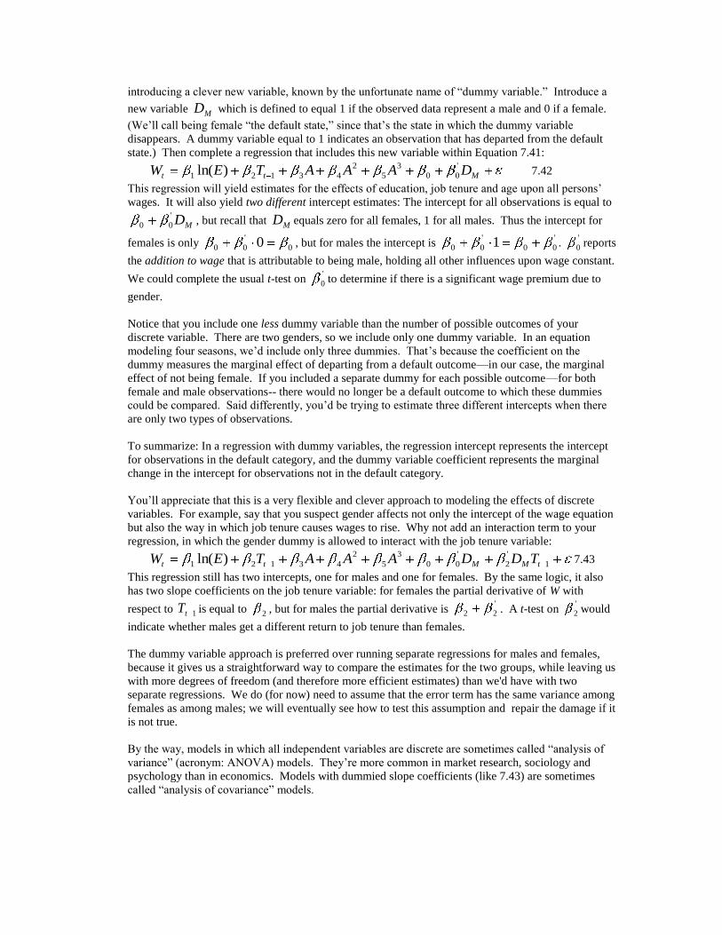
introducing a clever new variable, known by the unfortunate name of “dummy variable.” Introduce a

new variable MD which is defined to equal 1 if the observed data represent a male and 0 if a female.

(We’ll call being female “the default state,” since that’s the state in which the dummy variable

disappears. A dummy variable equal to 1 indicates an observation that has departed from the default

state.) Then complete a regression that includes this new variable within Equation 7.41:

Mtt DAAATEW '

00

3

5

2

43121 )ln( 7.42

This regression will yield estimates for the effects of education, job tenure and age upon all persons’

wages. It will also yield two different intercept estimates: The intercept for all observations is equal to

MD'

00 , but recall that MD equals zero for all females, 1 for all males. Thus the intercept for

females is only 0

'

00 0 , but for males the intercept is '

00

'

00 1 . '

0 reports

the addition to wage that is attributable to being male, holding all other influences upon wage constant.

We could complete the usual t-test on '

0 to determine if there is a significant wage premium due to

gender.

Notice that you include one less dummy variable than the number of possible outcomes of your

discrete variable. There are two genders, so we include only one dummy variable. In an equation

modeling four seasons, we’d include only three dummies. That’s because the coefficient on the

dummy measures the marginal effect of departing from a default outcome—in our case, the marginal

effect of not being female. If you included a separate dummy for each possible outcome—for both

female and male observations-- there would no longer be a default outcome to which these dummies

could be compared. Said differently, you’d be trying to estimate three different intercepts when there

are only two types of observations.

To summarize: In a regression with dummy variables, the regression intercept represents the intercept

for observations in the default category, and the dummy variable coefficient represents the marginal

change in the intercept for observations not in the default category.

You’ll appreciate that this is a very flexible and clever approach to modeling the effects of discrete

variables. For example, say that you suspect gender affects not only the intercept of the wage equation

but also the way in which job tenure causes wages to rise. Why not add an interaction term to your

regression, in which the gender dummy is allowed to interact with the job tenure variable:

1

'

2

'

00

3

5

2

43121 )ln( tMMtt TDDAAATEW 7.43

This regression still has two intercepts, one for males and one for females. By the same logic, it also

has two slope coefficients on the job tenure variable: for females the partial derivative of W with

respect to 1tT is equal to 2 , but for males the partial derivative is '

22 . A t-test on '

2 would

indicate whether males get a different return to job tenure than females.

The dummy variable approach is preferred over running separate regressions for males and females,

because it gives us a straightforward way to compare the estimates for the two groups, while leaving us

with more degrees of freedom (and therefore more efficient estimates) than we'd have with two

separate regressions. We do (for now) need to assume that the error term has the same variance among

females as among males; we will eventually see how to test this assumption and repair the damage if it

is not true.

By the way, models in which all independent variables are discrete are sometimes called “analysis of

variance” (acronym: ANOVA) models. They’re more common in market research, sociology and

psychology than in economics. Models with dummied slope coefficients (like 7.43) are sometimes

called “analysis of covariance” models.

Discrete Dependent Variables: Now consider a case in which all independent variables are

continuous, but the influence a dependent variable that is discrete. The most common case would be a

binary dependent variable.

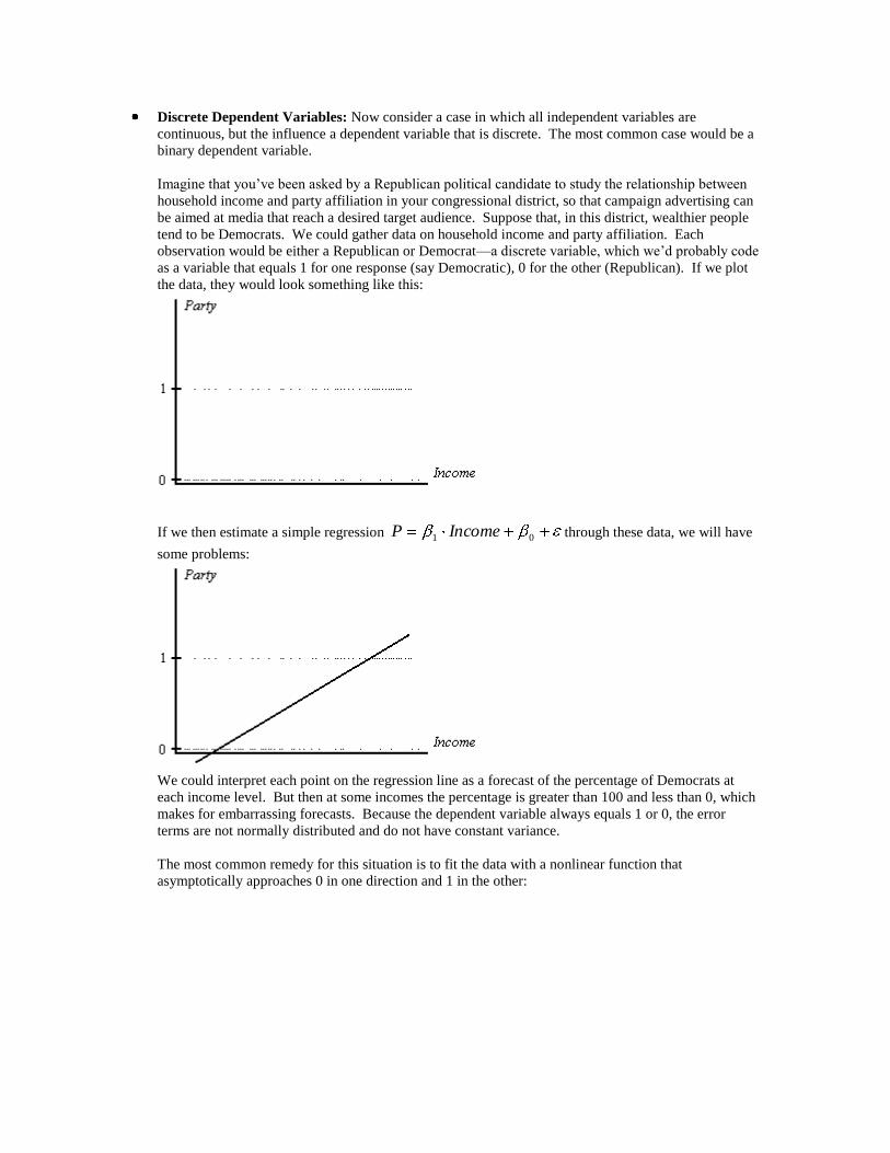
Imagine that you’ve been asked by a Republican political candidate to study the relationship between

household income and party affiliation in your congressional district, so that campaign advertising can

be aimed at media that reach a desired target audience. Suppose that, in this district, wealthier people

tend to be Democrats. We could gather data on household income and party affiliation. Each

observation would be either a Republican or Democrat—a discrete variable, which we’d probably code

as a variable that equals 1 for one response (say Democratic), 0 for the other (Republican). If we plot

the data, they would look something like this:

If we then estimate a simple regression 01 IncomeP through these data, we will have

some problems:

We could interpret each point on the regression line as a forecast of the percentage of Democrats at

each income level. But then at some incomes the percentage is greater than 100 and less than 0, which

makes for embarrassing forecasts. Because the dependent variable always equals 1 or 0, the error

terms are not normally distributed and do not have constant variance.

The most common remedy for this situation is to fit the data with a nonlinear function that

asymptotically approaches 0 in one direction and 1 in the other:

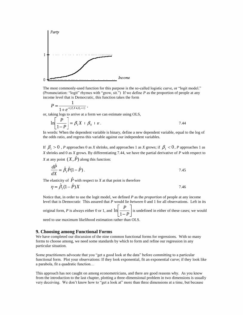
The most commonly-used function for this purpose is the so-called logistic curve, or “logit model.”

(Pronunciation: “logit” rhymes with “grow, sit.”) If we define P as the proportion of people at any

income level that is Democratic, this function takes the form

)( 011

1X

eP ,

or, taking logs to arrive at a form we can estimate using OLS,

011

ln XP

P. 7.44

In words: When the dependent variable is binary, define a new dependent variable, equal to the log of

the odds ratio, and regress this variable against our independent variables.

If 01 , P approaches 0 as X shrinks, and approaches 1 as X grows; if 01 , P approaches 1 as

X shrinks and 0 as X grows. By differentiating 7.44, we have the partial derivative of P with respect to

X at any point )ˆ,( PX along this function:

)ˆ1(ˆˆˆ

1 PPdX

Pd. 7.45

The elasticity of P with respect to X at that point is therefore

XP)ˆ1(ˆ1 7.46

Notice that, in order to use the logit model, we defined P as the proportion of people at any income

level that is Democratic This assured that P would lie between 0 and 1 for all observations. Left in its

original form, P is always either 0 or 1, and P

P

1ln is undefined in either of these cases; we would

need to use maximum likelihood estimation rather than OLS.

9. Choosing among Functional Forms We have completed our discussion of the nine common functional forms for regressions. With so many

forms to choose among, we need some standards by which to form and refine our regression in any

particular situation.

Some practitioners advocate that you “get a good look at the data” before committing to a particular

functional form. Plot your observations: If they look exponential, fit an exponential curve; if they look like

a parabola, fit a quadratic function…

This approach has not caught on among econometricians, and there are good reasons why. As you know

from the introduction to the last chapter, plotting a three-dimensional problem in two dimensions is usually

very deceiving. We don’t know how to “get a look at” more than three dimensions at a time, but because

we have no controlled lab we are usually dealing with problems that have many more than three variables

changing at once. In fact, you might say that we have been developing a technique for “looking at” more

than three dimensions at a time, by using symbols and algebra, and that technique is regression analysis.

(As we’ll learn in succeeding lessons, this makes it more important that you get a good look at your

regression residuals than looking at the data from which they come.)

Alternatively, in the age of high-powered computing, you could surrender you judgement to the machine

and simply ask the ether to try many different types of functional forms, and wake you up later with a

report of which one fit the data best. You’d have to define “best,” of course—presumably something like

“highest 2R .” There are many “curve-fitting” programs for this purpose. They may be appropriate in

some natural sciences, where one can control for changes in variables that are not under study. Even in

these non-econometrics cases we would be suspicious of merely “fitting the best curve to the data” with no

appeal to theory or knowledge about the situation under study. Taken to the extreme, this inductive

approach would merely list the data and quit! To be science, we normally want work to be theory-driven

and hypothesis-sifting, to be somewhat deductive rather than purely inductive. And in econometrics, where

no lab is available to control for changes in variables that are not under study, it’s the very presence and

influence of such rogue variables that we must identify and outwit. As we saw in the introduction to

Chapter 6, a badly-thought-through model can generate results that would look good to a computer and yet

tell us nothing at all about the actual situation we are trying to decipher.

Econometricians have therefore stuck with a detective-like process for seeking the best functional form,

starting with preliminary hypotheses and refining them as the data are analyzed. While the literature on

this topic is vast, we can give a general overview and introduce several of the most common statistical tests

that are involved.

Though we must often violate the first step in econometrics courses, in the name of considering a great

variety of models, there is no substitute for starting with a rich, detailed, normatively-sensitive

knowledge of the situation under study.

Your knowledge and intuition about the situation should be formed by relevant economic theory, so

that you propose a small number of most-likely forms for the regression equations. These amount to a

small number of competing hypotheses about the world. At the same time, you will be proposing

candidates for influential independent variables. As we’ve said earlier, the American instinct has been

to start with a relatively small model in which you have confidence and introduce more variables if

necessary, while the British have tended to start with larger models and whittle them down.

If you’re following the British instinct, we’ve already developed the relevant statistical tests by which

you can judge the statistical significance of an individual variable (the t-test) or group of restrictions

(the Wald test). This is a form of “specification testing,” in which we refine the specification of a

particular model. A rough rule of thumb is to drop variables whose statistical significance does not

meet your threshold. One commonly-accepted threshold is the 95% level of confidence, but exercise

caution if the variable’s t-statistic is greater than one.

If you’re following the American instinct, you may be wondering if there is a test to tell you whether

you should add a new variable or set of variables. Let’s consider one common test: the Lagrange

Multiplier test. Like the Wald test, this pits a restricted model against an unrestricted model, in which

the restricted model represents the null hypothesis.

The LM test follows this logic:

Say that we start with K potential explanatory variables, but hypothesize that only M of these are

statistically significant (that is, have a regression not equal to zero). First run the restricted

model regression, including only M variables, and save the residuals from it: m

k

kkR XYu1

0ˆ]ˆ[ˆ

The other, deleted K-M variables are actually part of the residual in this regression. If some of

them do affect Y (i.e., if 0H is unreasonable), their effect is therefore part of the residual. These

effects should therefore leave some evidence in the Ru if they indeed exist. We would detect

these effects by regressing the Ru against the omitted variables, looking for a good 2R as

evidence that some of the omitted variables indeed do “matter.”

As it turns out, the test’s distribution is simplified if we run this second regression of the Ru terms

against a constant term and all of the variables in the unrestricted model—both those that had been

excluded from the first regression, and those that were included. Under the null hypothesis, this

“auxiliary” regression’s 2R multiplied by the sample size N follows a

2

MK distribution—a chi-

square distribution with degrees of freedom equal to the number of restrictions. If 2RN exceeds

the appropriate critical value from the 2

table, we must reject the null hypotheses-- the excluded

variables explain too much in the residuals to conclude that they are not significant in the original

regression.

In that case, we’d then develop a larger regression than the restricted version, adding variables that

have good t-tests in the auxiliary regression. In fact, the coefficients and t-tests for the new K-M

variables in the auxiliary regression are identical to the coefficients and t-tests we’d get in a

completely unrestricted regression that includes all K variables.

To summarize: LM Test for 0i parameter restrictions: (K potential slope parameters, M parameters left

unrestricted, K-M restrictions) 7.47

0: 210 KmmH

:AH The restriction on at least one is untrue.

Process:

Regress all K variables against residuals from a restricted regression with M variables

T est Statistic under H0: 22 ~ MKauxiliaryRN

Decision Rule: Reject 0H if the calculated 2

statistic is greater than the appropriate

crirical value, or (equivalently) if the test’s p-value is less than the desired level of

significance.

To close this discussion of the LM test as a substitute for the Wald test, several cautions:

Neither Wald nor LM are useful for non-nested hypotheses, like asking if we should

simultaneously delete some variables and add others. Tests of such hypotheses are discussed, for

example, by Maddala, Introduction to Econometrics, 2nd

Ed., pp. 515ff..

While the Wald test is valid for any sample size, the LM test is valid only for large samples,

though its results may be approximate in sample sizes as small as 30.

Whether you are following the general-to-simple or the simple-to-general approach, there are other

forms of specification testing that check to see if our regression violates the basic assumptions about

the error term. We’ll encounter them in later chapters.

One would be especially concerned if the sign on a coefficient were the opposite of what you’d expect

from theory. This often indicates that the model is misspecified—perhaps an important variable has

been left out, so the remaining coefficients pick up it’s effects, or perhaps one of the eight basic

simplifying assumptions has been violated. (We will learn more about diagnosing violations of

assumptions in the following chapters.) In general, regressions with “wrong” signs are begging to be

re-thought.

Judging the relative value of two competing models (“model selection") can be more complicated

than the discussion we’ve been having about judging which variables to include in a model. As an

example, suppose you are deciding between a polynomial specification,

0

2

21 xxy 7.47

and a log-linear specification,

01)ln( xy 7.48

Your instinct may be to accept the model with the larger 2R value, but that is an imperfect approach,

especially in a case like this where we’re comparing two models in which the dependent variable is

not identical. In the first case, 2R measures the proportion of variation in y explained by x, whereas

in the second 2R measures the proportion of variation in ln(y) explained by x. We can make the two

comparable by adjusting 2R in the second equation:

Obtain the fitted values of )ln(y from the regression results.

Use these to compute an estimated average value for y by taking antilogs and making the bias

adjustment we suggested in Equation 7.26:

)2

ˆ()ln(2

ˆ ny

n ey

Calculate the square of the correlation between ny and ny , which is directly comparable to the

2R of regression 7.47.

For computing an 2R or

2ˆ that can be compared to Regression 7.47, you’ll need to first

calculate a modified ESS for this model:

n

nn yyESS 2)ˆ( , )1(

ˆ 2

kN

ESS7.49

Rather than judge models by comparing their2R values, we could (especially in situations where

forecasting is a goal of the study) judge models by their ability to predict the dependent variable. We

might calculate competing models’ MSE or RMSE for observations that were withheld when

estimating the regression, and choose the model with the lower forecast error. This approach is

formalized into several regression-evaluation statistics produced by most statistical programs--among

them Mallows’ pC criterion, Hocking’s pS criterion, and Amemiya’s PC criterion.

Finally, we should consider the “test of an unknown misspecification,” Ramsey’s RESET (regression

specification error test). Recall from our discussion of the LM test that the effect of omitted variables

is felt, if at all, in the regression residuals. If there’s no missing-variable-effect there to notice, the

residuals should just be white noise that follows no pattern. The LM test searches for a pattern in the

residuals that is a function of some potential independent variables we’ve identified. How could we

search for a pattern without identifying any particular potential explanatory variables? We can search

for a pattern that’s a function of the predicted values of the dependent variable. If the error terms are a

systematic function of the predicted values of Y, then there’s something systematic in Y’s changes that

is not yet explained by our regression, so the regression is not properly specified. Ramsey suggests we

use a fourth-degree polynomial for the form of the auxiliary regression: RESET Test for regression specification error 7.50

:0H The regression is correctly specified.

:AH The regression is not correctly specified.

Process:

Save the fitted nY values from the regression.

Modify this regression by adding 2ˆ

nY , 3ˆ

nY and 4ˆ

nY as explanatory variables.

Estimate this expanded regression (using the original Y as dependent variable).

In the final regression, complete a Wald test for significance of the three added variables.

T est Statistic under H0: )1(,3~

..3

)(

KN

U

U

UR

F

fd

ESSESSESS

Decision Rule: Reject 0H if the calculated F statistic is greater than the appropriate critical

value, or (equivalently) if the test’s p-value is less than the desired level of significance.

If you sense irony in my statement of the null and alternative hypotheses, you are not inventing it. The

test does not indicate what kind of misspecification has taken place, so it doesn’t tell us much about

what we should do. But the test can at least suggest that we need to rethink our model and gather some

more information.

10. Preview In this chapter we’ve introduced a number of functional forms for regressions, and suggested a general

process for judging which form is appropriate in any particular situation. This was all a way of relaxing the

first simplifying assumption that we made in Chapter Five, because not all real relationships are linear.

There are just a few more topics that we will discuss in this course:

Diagnosis, prognosis and treatment of violations of our basic assumptions about the error term: Heteroscedasticity and Serial Correlation (Basic Assumptions Four and Five)

Diagnosis, prognosis and treatment of violations of our basic assumptions about independent variables: Multicollinearity (Basic Assumption Seven)

Time-Series Modeling and Forecasting Simultaneous Equation Models

If you’re being very thorough, you’ll notice that this leaves several basic assumptions not thoroughly

explored, most notably number three (X variables measured without error) and number six (normality of

errors). You’ll find a discussion of number three in most advanced econometrics texts under the heading

“errors in variables” or “instrumental variables.” Because of the sources of the regression error, the

conditions of the central limit theorem generally (at least approximately) apply, and (except in special cases

when circumstances clearly require a different assumption) assumption six is generally thought to be

reasonable. For the skeptical, Greene suggests a test for normality based on the skew and kurtosis of the

regression residuals: Econometric Analysis, 4th

Ed., p. 161, #15.