Chapter 6: State-space Analysis & Design Outline Concept of state, state variable and model • What are state-space models? • Why should we use them ? • How are they related to the TFs? System response from State space model • State transition matrix • eigenvalues & eigenvectors State feedback controller design • Concept of controllability & Obserivability State estimator design 1

Chapter 6 State Space Analysis
Nov 27, 2015
State space analysis
Welcome message from author
This document is posted to help you gain knowledge. Please leave a comment to let me know what you think about it! Share it to your friends and learn new things together.
Transcript

1
Chapter 6: State-space Analysis & Design
OutlineConcept of state, state variable and
model • What are state-space models?• Why should we use them ?
• How are they related to the TFs?System response from State space model
• State transition matrix
• eigenvalues & eigenvectors State feedback controller design
• Concept of controllability & ObserivabilityState estimator design

2
Chapter 6: State-space Analysis & Design
[6.1] State Concept:
The state of a dynamical system is a minimum set of variables ( known as state variables, x(t) ) such that the knowledge of theses variables at together with the knowledge of the input for completely determines the behavior of the system for
x(t) is called state of the system at t because: • Future output depends only on current state and future input• Future output depends on past input only through current state• State summarizes effect of past inputs on future output-like the memory of the system
0tt
0tt
0tt
Figure 6.1 Structure of general control system
:
Controlled SystemState variable
Output variabl
es
Inputvariabl
es
:..

3
Chapter 6: State-space Analysis & Design
SS Introduction: State space model: a representation of the
dynamics of an Nth order system as a first order differential equation in an N-vector, which is called the state. • Convert the Nth order differential equation
that governs the dynamics into N first-order differential equations.
Example 5.1: For the mechanical system shown below find the differential equation relating u & y. For the same find SS representation
Figure 6.2 Second order mass-spring system

4
Chapter 6: State-space Analysis & Design
Solution:
• Let , then , and
( )• If the measured output of the system
( Example 5.1) is the position, then we have that

5
Chapter 6: State-space Analysis & Design
• Most general continuous-time linear dynamical system has form
Where• is the state ( vector) • is the input or control • is the output• is the dynamics matrix• is the input matrix• is the output or sensor matrix• is the feedthrought matrix

6
Chapter 6: State-space Analysis & Design
We will typically deal with the time-invariant case Linear Time-Invariant (LTI) stat dynamics So that now A,B,C,D are constant and don’t depend on t.
∫B ++
A
C ++
D
u y
Figure 6.3 Block diagram representation of the state model of a linear time invariant MIMO system

7
Chapter 6: State-space Analysis & Design
Why should we use SS Model ?
• State variable form convenient way to work with complex dynamics. Matrix format easy to use on computers.
• Transfer function only deal with input/output behavior, but state-space form provides easy access to the “internal” features/response of the system.
• Allow us to explore new analysis and synthesis tools.
• Great for multiple-input multiple-output systems(MIMO), which are very hard to work with using transfer functions.
• Easy to study/design optimal control systems.

8
Chapter 6: State-space Analysis & Design
[6.2] System response from State Space Model
Consider the classical method of solution by considering a 1st –order scalar DE:
Let us now consider the state space equation:
;
Which represents a HOMOGENEOUS ( unforced ) Linear system with constant coefficients.
By analogy with the scalar case, we assume a solution of the form
Where are vector coefficients.
[6.1]
[6.2]
[6.3]

9
Chapter 6: State-space Analysis & Design
[6.2] System response from State Space Model
Substituting the assumed solution into [6.3] gives
Equating coefficients of equal powers of t, yields
In the assumed solution, equating , we find that
the solution of X(t) is thus found to be
:.
:.
[6.4]
10
Chapter 6: State-space Analysis & Design
[6.2] System response from State Space Model
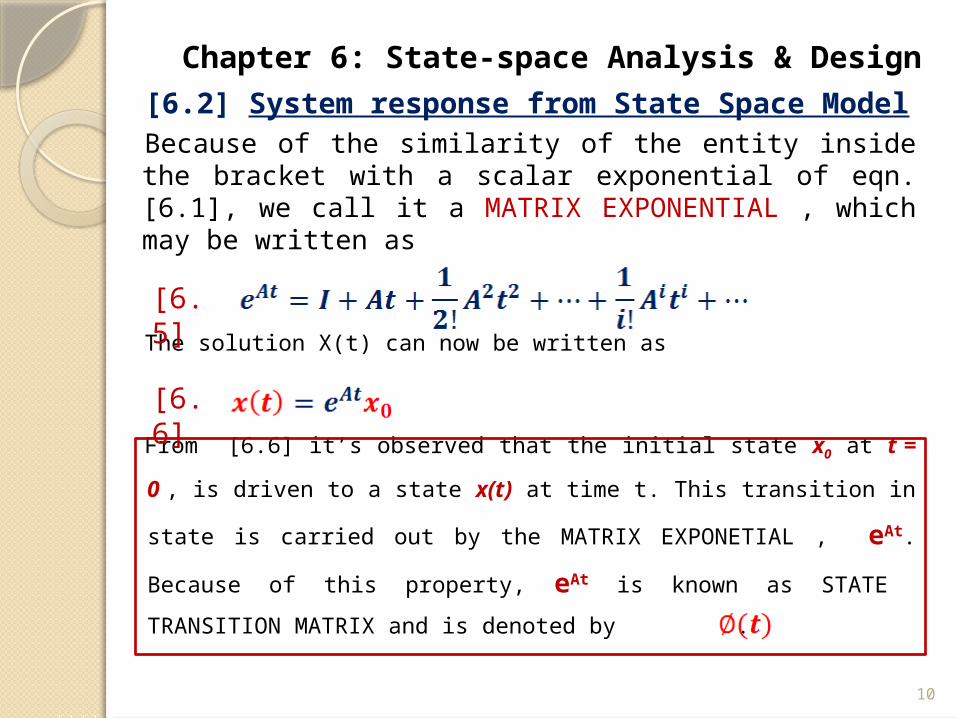
Because of the similarity of the entity inside the bracket with a scalar exponential of eqn.[6.1], we call it a MATRIX EXPONENTIAL , which may be written as
The solution X(t) can now be written as
From [6.6] it’s observed that the initial state x0 at t = 0 , is
driven to a state x(t) at time t. This transition in state is carried
out by the MATRIX EXPONETIAL , eAt. Because of this property,
eAt is known as STATE TRANSITION MATRIX and is denoted by
.
[6.5]
[6.6]
11
Chapter 6: State-space Analysis & Design
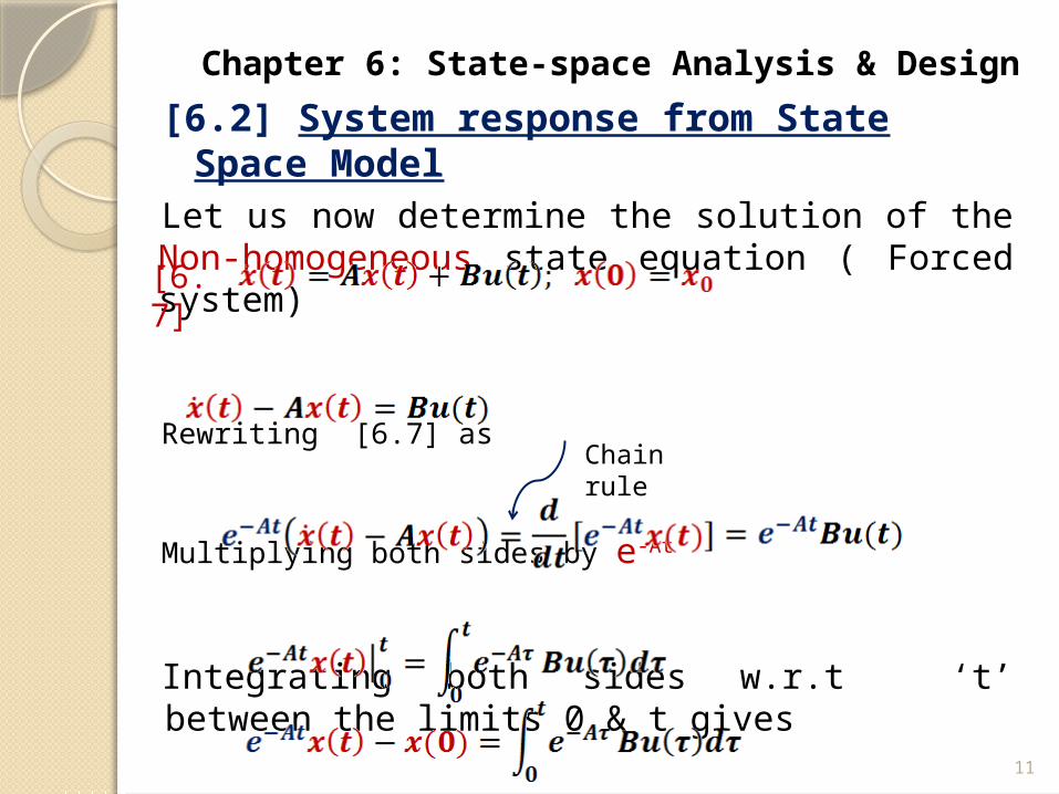
[6.2] System response from State Space Model
Let us now determine the solution of the Non-homogeneous state equation ( Forced system)
Rewriting [6.7] as
Multiplying both sides by e-At
Integrating both sides w.r.t ‘t’ between the limits 0 & t gives
[6.7]
Chain rule

12
Chapter 6: State-space Analysis & Design
[6.2] System response from State Space Model
Now pre-multiplying both sides by eAt , we have
Properties of the State Transition Matrix
(i)
(ii)
or
(iii)
[6.8]
Homogeneous solution
Forced solution

04/17/2023 13
Chapter 6: State-space Analysis & Design
How to Compute State transition Matrix ?
• Laplace transformation• Cayley-Hamilton Theorem• Infinite sum series• Similarity transformation method• And other methods ( 15 more)
Cayley-Hamilton TheoremAssume we are given and an matrix with characteristics polynomial
Where
Define
14
Chapter 6: State-space Analysis & Design
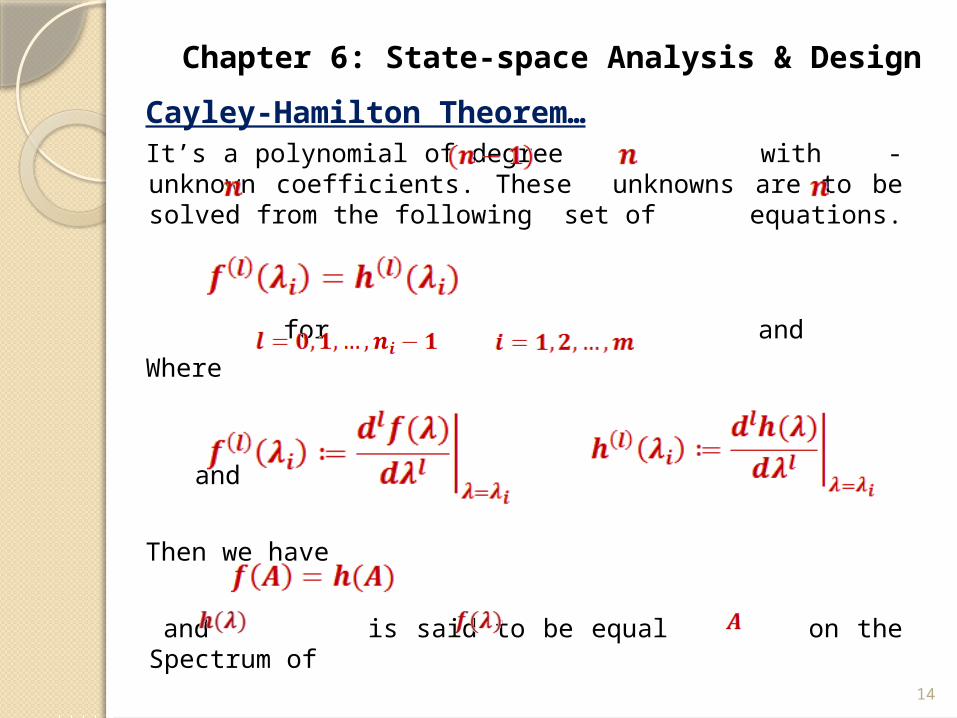
Cayley-Hamilton Theorem…It’s a polynomial of degree with - unknown coefficients. These unknowns are to be solved from the following set of equations.
for and
Where
and
Then we have
and is said to be equal on the Spectrum of

15
Chapter 6: State-space Analysis & Design
Cayley-Hamilton Theorem…
Example 6.2 : Compute the ‘fundamental matrix/state transition matrix of A’, where
Using Cayley-Hamilton Theorem.
Solution:The problem is given what is
•The characteristics polynomial of is the solution of the
equation
or

16
Chapter 6: State-space Analysis & Design
Cayley-Hamilton Theorem…
Example 6.2 …
Let
Then applying Cayley-Hamilton Theorem, we have
• ;
• ;
Solving these simultaneous equations using Gauss’s elimination technique, i.e.,

17
Chapter 6: State-space Analysis & Design
Cayley-Hamilton Theorem…
Example 6.2 …
• Back substitution gives
;
•Thus ,

18
Chapter 6: State-space Analysis & Design
Cayley-Hamilton Theorem…
Exercise: For the Matrix A, given below , compute the state transition matrix using Cayley-Hamilton Theorem.
Answer: Same as to that of Example 6.2.
Q. What is your conclusion?
Remark:
If two system matrix have same characteristics polynomial then their state transition matrix is the same. The two system matrix are called similar.

19
Chapter 6: State-space Analysis & Design
Eigenvalues & Eigenvectors is an eigenvalue of if , which is true iff there exist
a nonzero ( eigenvector) for which
Repeat the process to find all of the Eigenvectors, i.e.,
;
Example 6.3
Compute the eigenvalues & eigenvectors for the system given by

20
Chapter 6: State-space Analysis & Design
Eigen Values & Eigenvectors…Example 6.3…
• Eigenvectors:
Note , Either or can be chosen arbitrarily. So let
Similarly,
, choose

21
Chapter 6: State-space Analysis & Design
Eigen Values & Eigenvectors…Remark: The locations of the eigenvalues determine the pole locations for the system, thus; • they determine the stability and /or performance & transient behavior of the system• It is their locations that we want to modify when we start controller design work.• for stability, • For steady-state to exist one of must be equal to Zero and the other
22
Chapter 6: State-space Analysis & Design
[6.3] State Feedback Controller DesignOur focus:
State feedback control law design to satisfy specified closed loop performance in terms of both transient and steady-state response characteristics.
Preliminaries concepts:
State Controllability:
-the ability to manipulate the state by applying appropriate inputs ( in particular , by steering the state vector ) from one vector value to any other vector value in finite time.
State Observability:
- the ability to determine the state vector of the system from the knowledge of the input and the corresponding output over some finite time interval.

23
Chapter 6: State-space Analysis & DesignMathematical condition for State Controllability
& Observability
(6.9)
The system in (6.9) is controllable if the Controllability Matrix, U has full rank (i.e., det U ≠ 0)
Where U is given by
(6.10)
Similarly, the system in (6.9) is state observable if the Observability Matrix, V has full rank ( i.e., det(V) ≠ 0)
Where V is given by
(6.11)

24
Chapter 6: State-space Analysis & Design
Full State Feedback Controller Design
Recall that the system poles are given by the eigenvalues of A
- want to use the input u(t) to modify the eigenvalues of A to change
the system dynamics
• Assume a full-state feedback of the form
(6.12)
Where is some reference input
A, b, C
K
+- r
y x(t)

25
Chapter 6: State-space Analysis & Design
Full State Feedback Controller Design…
• Find the closed-loop dynamics
;
and
• Objective
Pick K so that have the desired properties, e.g., making unstable (A) into stable , putting 2 poles @ say
A, b, C
K
+- r
y x(t)

Chapter 6: State-space Analysis & Design
Full State Feedback Controller Design…
Example 6.4 consider the dynamical system given below
Following the previous outlined procedure , we have
So that
Thus , the FB control law can modify the pole @ s = 1, but it can’t move the pole @ s =2
This system can’t be Stabilized with full-state feedback control law
26

Chapter 6: State-space Analysis & Design
Full State Feedback Controller Design…
Reference Input
• so far we have looked at how to pick K to get the dynamic to have some nice properties(i.e., Stabilize A)
• The question remains as to how well this controller allows us to track a reference command ?
- performance issue rather than just stability
• For good tracking performance we want
Start with
27

Chapter 6: State-space Analysis & Design
Full State Feedback Controller Design…
Reference Input …
Consider this performance issue in the frequency domain. From the final value theorem:
Thus, for good performance , we want
So , for good performance , the transfer function from R(s) to Y(s) should be approximately 1 at DC (i.e., @ s=0)
28
Chapter 6: State-space Analysis & Design
Full State Feedback Controller Design…
Reference Input …
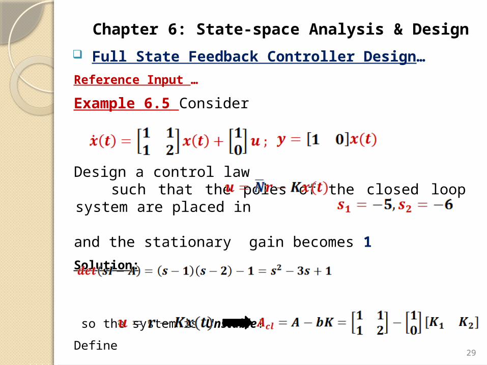
Example 6.5 Consider
Design a control law such that the poles of the closed loop system are placed in and the stationary gain becomes 1
Solution:
so the system is Unstable!
Define29

Chapter 6: State-space Analysis & Design
Full State Feedback Controller Design…
Reference Input …
Example 6.5…
Which gives
• To put the poles at , compare the desired characteristics equation, i.e.,
•With the closed-loop one
; ; 30
Chapter 6: State-space Analysis & Design
Full State Feedback Controller Design…
Reference Input …
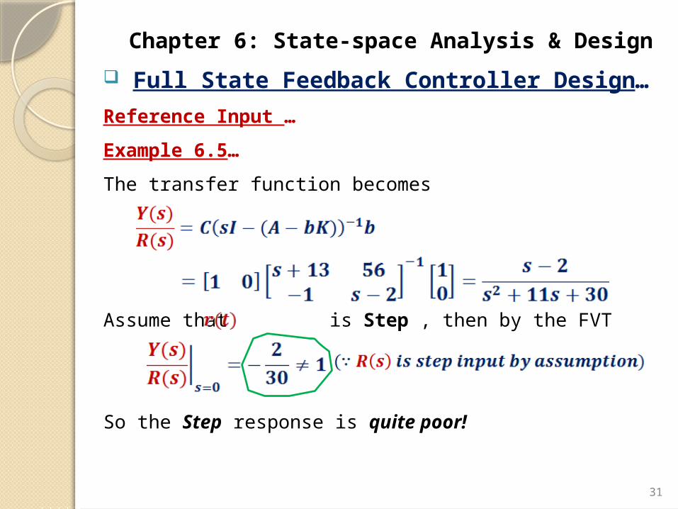
Example 6.5…
The transfer function becomes
Assume that is Step , then by the FVT
So the Step response is quite poor!
31
Chapter 6: State-space Analysis & Design
Full State Feedback Controller Design…
Reference Input …
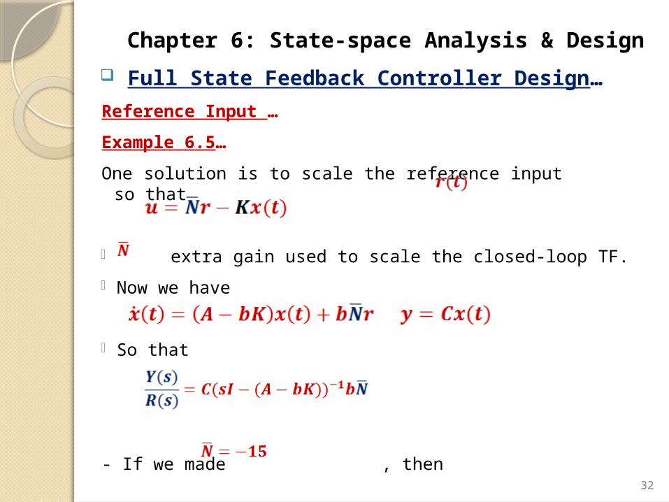
Example 6.5…
One solution is to scale the reference input so that
- extra gain used to scale the closed-loop TF.
- Now we have
- So that
- If we made , then
32

Chapter 6: State-space Analysis & Design
Full State Feedback Controller Design…
Reference Input …
Example 6.5…
So with a step input,
33

Chapter 6: State-space Analysis & Design
[6.4] Full-state Observer/Estimator DesignThe State feedback in the preceding section is introduced under the assumption that all state variables are available for connection to a gain. However, this assumption may or may not hold in practice
Figure 6.4 Open-loop state estimator 34
to be implemented via software
+u
y
+

Chapter 6: State-space Analysis & Design
Open-loop State estimator
Let the output of the Estimator/Observer in Figure 6.4 be denoted by
Then the system in Figure 6.4 can be described by
(6.13)
Subtracting (6.13) from (6.9a) gives
Let define state estimation error as
Then it’s governed by
(6.14)
And its solution is
35

Chapter 6: State-space Analysis & Design
Open-loop State estimator…
Note:• Even if all eigenvalues of A has negative real parts, we have no control over the rate at which approaches zero. Hence rarely used in practice.• Although the output is available , it is not utilized in the open-loop estimator in Figure 6.4.
Alternative Approach/ Strategy• Feedback the difference ( i.e., ) to improve our estimate of the state.
Closed-loop State Estimator/Observer
36

Chapter 6: State-space Analysis & Design
Closed-loop State Estimator/Observer
++
+
- +
37

Chapter 6: State-space Analysis & Design
Closed-loop State Estimator/Observer…
The output of the ESTIMATOR is governed by
Or
(6.16)
Remark:
If (A, C) is observable , the (6.16) can be designed so that the estimated state will approach the actual state as quickly as desired. • Subtracting (6.16) from (6.9a) gives ( noting )
Or equivalently,
(6.17) 38

Chapter 6: State-space Analysis & Design
Closed-loop State Estimator/Observer…
Bottom line:
• Can select the gain L to attempt to improve the convergence of the estimation error ( and/or speed it up)
• Estimator problem becomes choosing/designing such the closed-loop poles
are in the desired locations.
Example 6.6
For the system given below
39

Chapter 6: State-space Analysis & Design
Closed-loop State Estimator/Observer…
Example 6.6…
Design a full-order state observer/estimator, assuming the desired eigenvalues of the observer matrix are -10.
Solution:• the characteristics equation for the observer is given by
•Define
•then , the characteristics equation becomes
40

Chapter 6: State-space Analysis & Design
Closed-loop State Estimator/Observer…
Example 6.6…
• Since the desired characteristics equation is
• Comparing the two characteristics equations gives
41
Related Documents