Chapter 6 Business and Economic Forecasting Root-mean-squared Forecast Error zUsed to determine how reliable a forecasting technique is. zE = (Y i -

Chapter 6 Business and Economic Forecasting

Root-mean-squared Forecast Error

Used to determine how reliable a forecasting technique is.

E = (Yi - Fi)2 / n

where: Fi = ith forecast

Yi = the corresponding actual value

n = the number of forecasts

i=1

n

Taking Apart a Time Series

Trend: A relatively smooth long-term movement of a time-series.

The value of a variable might differ from trend because of:

Seasonal variationCyclical variationIrregular variation

Estimating a Linear Trend

Yt = A + Bt

where Yt is the trend value of the variable

at time t.

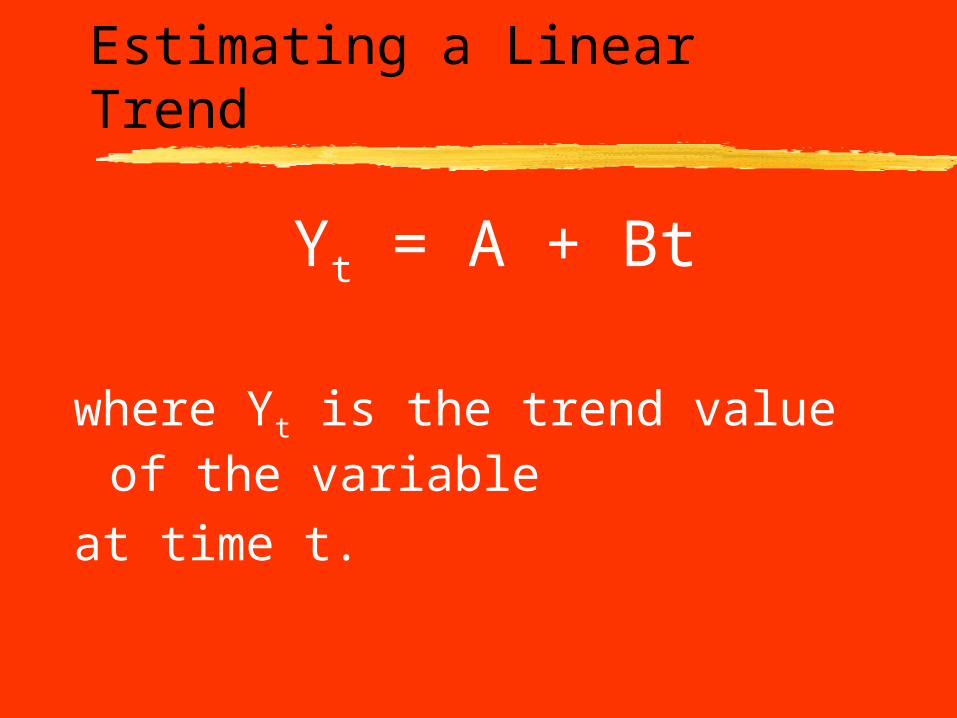
Estimating a Nonlinear Trend

Quadratic function

Yt = A + B1t + B2t2

Exponential function

Yt = t

or

log Yt = log a + log b x t

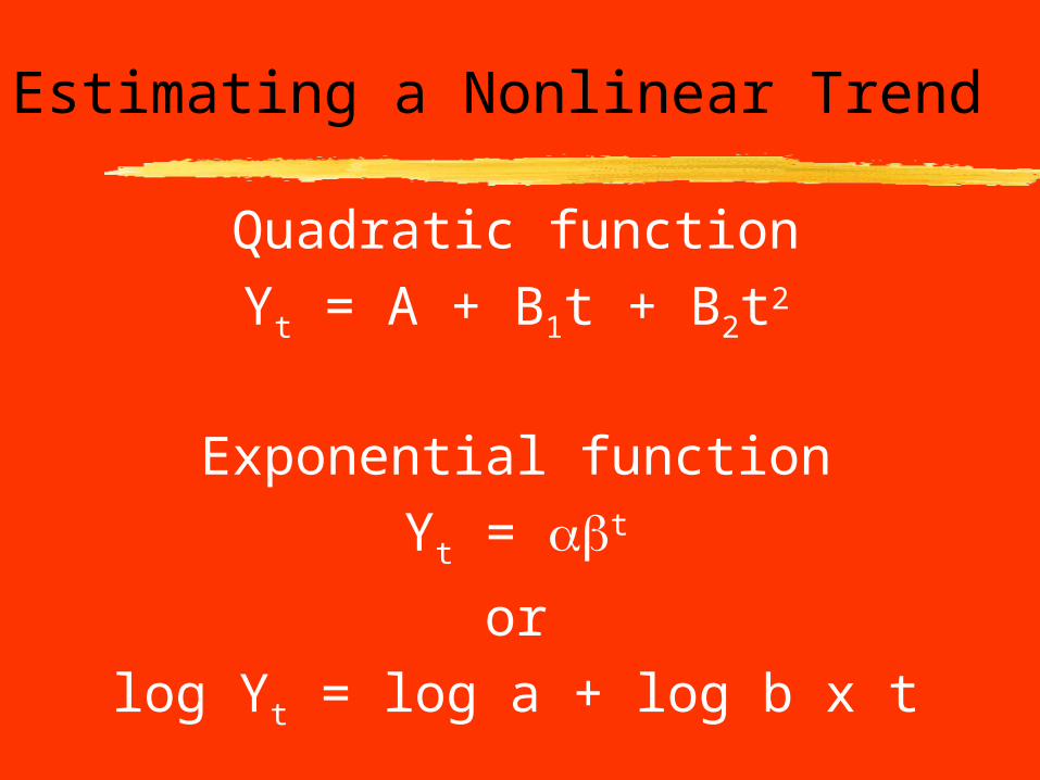
Accounting for Seasonal Variation

Seasonal indexDescribes the seasonal variation in a particular time

series Shows the way in which that month tends to depart

from what would be expected on the basis of the trend and cyclical variation in the time series

Accounting for Cyclical Variation

Business cycle: describes fluctuations in the level of economic activity over time

Time

Level of economic

activity

Trough

Peak

Expansion Contraction

Elementary Forecasting

Fundamental forecasting equation:

Yt=T x S x C x I

Trend Seasonal Effect Cyclical Effect Irregular Effect

Linear Trend

Shows the simple, linear effects of time on the dependent variable:

Yt= a + bt + et

Where t is our time index and et is our forecasting error.

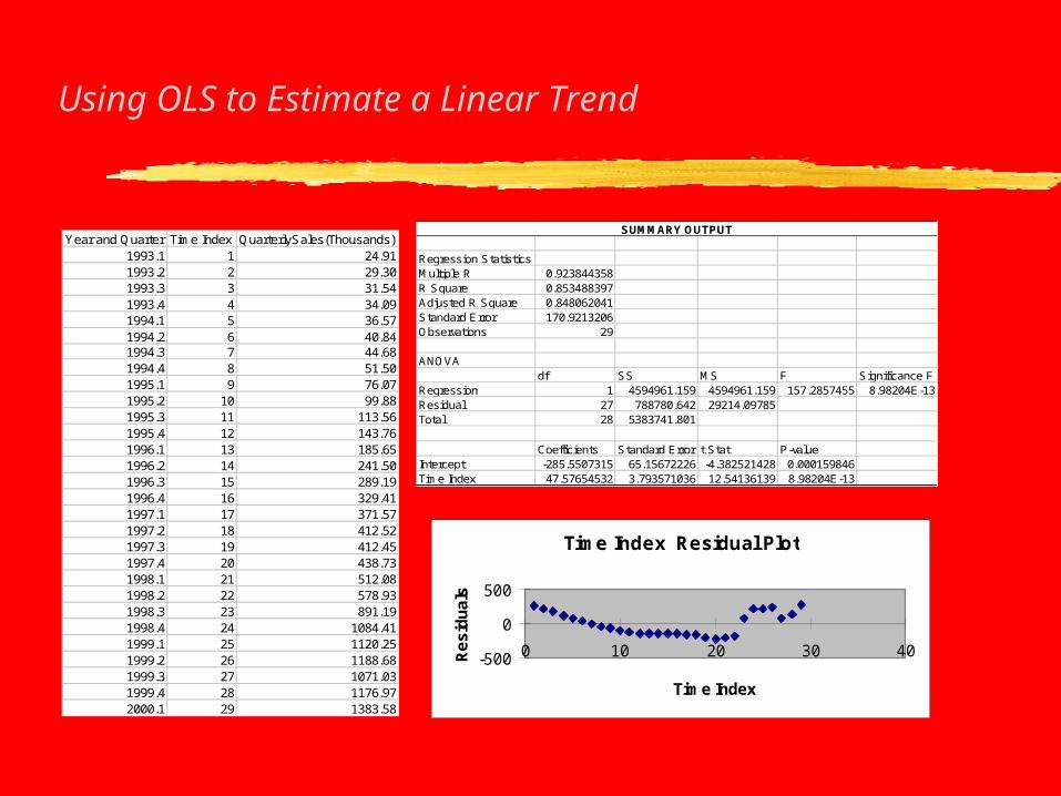
Using OLS to Estimate a Linear Trend

SUMMARY OUTPUT

Regression StatisticsMultiple R 0.923844358R Square 0.853488397Adjusted R Square 0.848062041Standard Error 170.9213206Observations 29

ANOVAdf SS MS F Significance F

Regression 1 4594961.159 4594961.159 157.2857455 8.98204E-13Residual 27 788780.642 29214.09785Total 28 5383741.801

Coefficients Standard Error t Stat P-valueIntercept -285.5507315 65.15672226 -4.382521428 0.000159846Time Index 47.57654532 3.793571036 12.54136139 8.98204E-13

Time Index Residual Plot

-500

0

500

0 10 20 30 40

Time Index

Re

sid

ua

ls

Year and Quarter Time Index QuarterlySales(Thousands)1993.1 1 24.911993.2 2 29.301993.3 3 31.541993.4 4 34.091994.1 5 36.571994.2 6 40.841994.3 7 44.681994.4 8 51.501995.1 9 76.071995.2 10 99.881995.3 11 113.561995.4 12 143.761996.1 13 185.651996.2 14 241.501996.3 15 289.191996.4 16 329.411997.1 17 371.571997.2 18 412.521997.3 19 412.451997.4 20 438.731998.1 21 512.081998.2 22 578.931998.3 23 891.191998.4 24 1084.411999.1 25 1120.251999.2 26 1188.681999.3 27 1071.031999.4 28 1176.972000.1 29 1383.58

Example: Fitting a Linear Trend (continued)

The forecasted equation is:thus, to forecast the 30th period we insert 30 in place of

t,

Notice that the errors seem not to be random, but we witness strings of positive errors and strings of negative errors. This is typically indicative of two possible problems: autorcorrelation or mis-specified functional form. We can consider the latter by plotting the data and looking for a non-linear pattern in the data.

47.58t-285.55Yt

85.114147.58(30)-285.55Y30

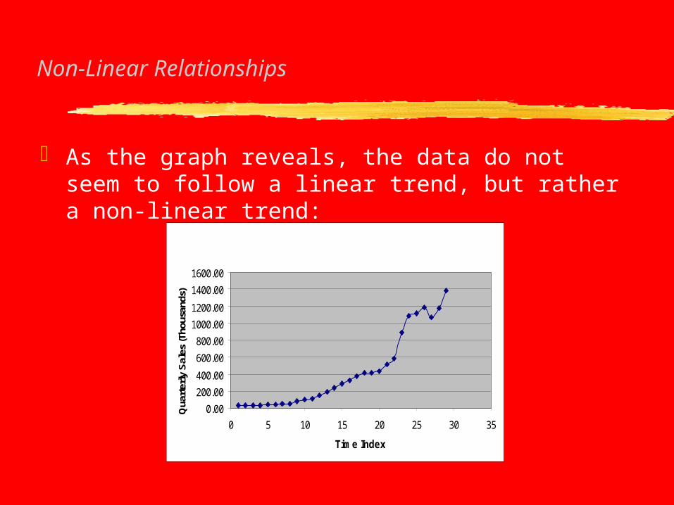
Non-Linear Relationships

As the graph reveals, the data do not seem to follow a linear trend, but rather a non-linear trend:

0.00

200.00

400.00

600.00

800.00

1000.00

1200.00

1400.00

1600.00

0 5 10 15 20 25 30 35

Time Index

Qua

rter

ly S

ales

(Tho

usan

ds)

Exponential and Polynomial Trends

Two common non-linear trend relationships:

Exponential: Yt= t

Polynomial: Yt= a + b1t + b2t2

(quadratic form)

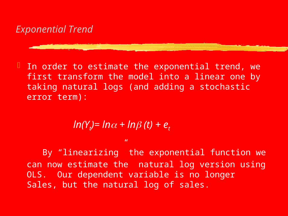
Exponential Trend

In order to estimate the exponential trend, we first transform the model into a linear one by taking natural logs (and adding a stochastic error term):

ln(Yt)= ln + ln (t) + et

By “linearizing” the exponential function we can now estimate the natural log version using OLS. Our dependent variable is no longer Sales, but the natural log of sales.

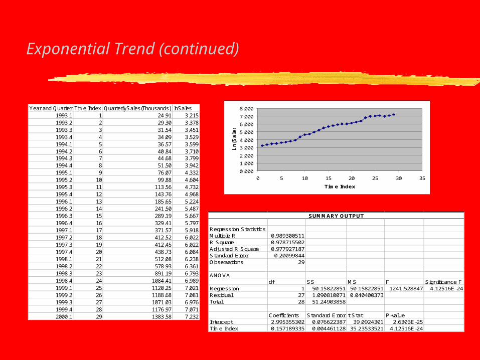
Exponential Trend (continued)

Year and Quarter Time Index QuarterlySales(Thousands) lnSales1993.1 1 24.91 3.2151993.2 2 29.30 3.3781993.3 3 31.54 3.4511993.4 4 34.09 3.5291994.1 5 36.57 3.5991994.2 6 40.84 3.7101994.3 7 44.68 3.7991994.4 8 51.50 3.9421995.1 9 76.07 4.3321995.2 10 99.88 4.6041995.3 11 113.56 4.7321995.4 12 143.76 4.9681996.1 13 185.65 5.2241996.2 14 241.50 5.4871996.3 15 289.19 5.6671996.4 16 329.41 5.7971997.1 17 371.57 5.9181997.2 18 412.52 6.0221997.3 19 412.45 6.0221997.4 20 438.73 6.0841998.1 21 512.08 6.2381998.2 22 578.93 6.3611998.3 23 891.19 6.7931998.4 24 1084.41 6.9891999.1 25 1120.25 7.0211999.2 26 1188.68 7.0811999.3 27 1071.03 6.9761999.4 28 1176.97 7.0712000.1 29 1383.58 7.232

0.000

1.000

2.000

3.000

4.000

5.000

6.000

7.000

8.000

0 5 10 15 20 25 30 35

Time Index

Ln

(Sa

les)

SUMMARY OUTPUT




Coefficients Standard Error t Stat P-valueIntercept 2.995355302 0.076622387 39.0924301 2.6303E-25Time Index 0.157189335 0.004461128 35.23533521 4.12516E-24

Exponential Trend (continued)

The estimate equation is:

thus the forecasted sales for the 30th. period would be:

( A simpler way to estimate this trend is to use the Excel Chart option and add an exponential trend line.)

t1572.09954.2)tsalesln(

667.2233)7114.7exp(30Sales

,or

7114.7)30(1572.09954.2)30

Salesln(

y = 19.992e0.1572x

R2 = 0.9787

0.00

500.00

1000.00

1500.00

2000.00

2500.00

0 5 10 15 20 25 30 35

Time Index

Qua

rterly

Sal

es (T

hous

ands

)

Quadratic Trend

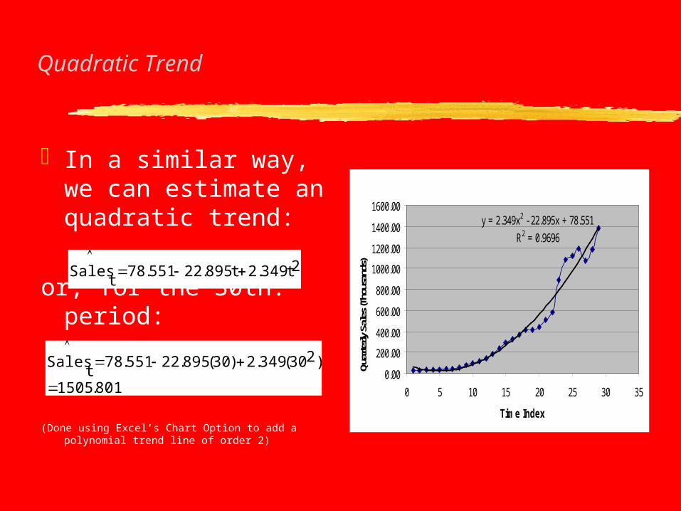
In a similar way, we can estimate an quadratic trend:

or, for the 30th. period:

(Done using Excel’s Chart Option to add a polynomial trend line of order 2)

y = 2.349x2 - 22.895x + 78.551

R2 = 0.9696

0.00

200.00

400.00

600.00

800.00

1000.00

1200.00

1400.00

1600.00

0 5 10 15 20 25 30 35

Time Index

Quar

terly

Sal

es (T

hous

ands

)2t349.2t895.22551.78t

Sales

801.1505

)230(349.2)30(895.22551.78t

Sales

Dummy Variables

A variable that can assume only two values:

0 or 1

Seasonal Adjustments Using Dummy Variables

One method of controlling for Season variation is to create seasonal dummy variables. Dummy variables, (also known as indicator or categorical variables), are simply variables that are created to indicate whether something is true. For example,

Yt= a + b1 t + b2D2t + b3D3t + b4D4t +et

Yt = monthly salest = time indexD2t = 1 is the month belongs to the 2nd quarter, 0 otherwise

D3t = 1 is the month belongs to the 3rd quarter, 0 otherwise

D4t = 1 is the month belongs to the 4th quarter, 0 otherwise

Using Dummy Variables (continued)

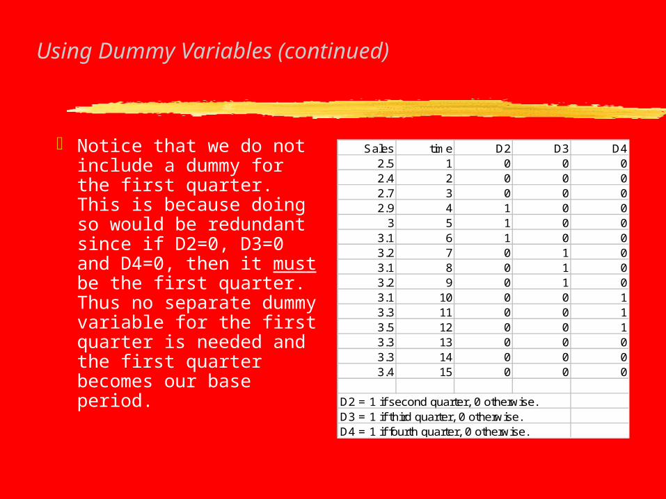
Notice that we do not include a dummy for the first quarter. This is because doing so would be redundant since if D2=0, D3=0 and D4=0, then it must be the first quarter. Thus no separate dummy variable for the first quarter is needed and the first quarter becomes our base period.

Sales time D2 D3 D42.5 1 0 0 02.4 2 0 0 02.7 3 0 0 02.9 4 1 0 0

3 5 1 0 03.1 6 1 0 03.2 7 0 1 03.1 8 0 1 03.2 9 0 1 03.1 10 0 0 13.3 11 0 0 13.5 12 0 0 13.3 13 0 0 03.3 14 0 0 03.4 15 0 0 0

D2 = 1 if second quarter, 0 otherwise.D3 = 1 if third quarter, 0 otherwise.D4 = 1 if fourth quarter, 0 otherwise.


SUMMARY OUTPUT




Coefficients Standard Error t Stat P-valueIntercept 2.391740413 0.061546059 38.86098412 3.03966E-12time 0.067699115 0.00610395 11.091034 6.10565E-07D2 0.269764012 0.067420329 4.001226544 0.002513355D3 0.233333333 0.064885877 3.596057344 0.004879751D4 0.163569322 0.067420329 2.42611276 0.035686645

OLS may be applied to this model and the dummy variables are treated as any other independent variable in the regression. The adjusted R squared increases substantially (from 0.792 without the dummies to 0.918 with them) indicating a better fit.


The predicted equation is,

Predicting the 16th. month’s sales, given it is a second quarter observation, we have:

4t0.164D3t

0.233D2t

0.270D0.0677t 2.392tSales

745.30.164(0)0.233(0)0.270(1)0.0677(16) 2.39216

Sales

Exponential Smoothing

Another method of forecasting values of a variable is to use a weighted average of previous values. This is precisely what exponential smoothing does. The “exponential” part of exponential smoothing refers to how the weights are assigned to previous values. The weights are assigned such that they decline exponentially as we move backward in time.

Exponential Smoothing (continued)

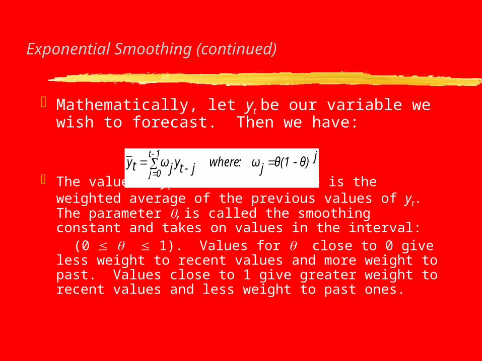
Mathematically, let yt be our variable we wish to forecast. Then we have:

The value of yt with the bar above is the weighted average of the previous values of yt. The parameter , is called the smoothing constant and takes on values in the interval:

(0 1). Values for close to 0 give less weight to recent values and more weight to past. Values close to 1 give greater weight to recent values and less weight to past ones.

jθ)θ(1jω:wherej-tyjωty1t

0j


The steps for forecasting go as the following;

1. Initialize:

2. Update:

3. Forecast:

1y1y:1t

2....Tt1-ty1yty ,)1(

ty1ty


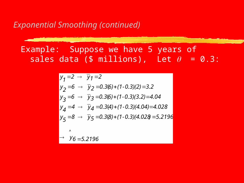
Example: Suppose we have 5 years of sales data ($ millions), Let = 0.3:

5.21966y

5.2196)0.3)(4.028-(18)0.35y85y

4.0280.3)(4.04)-(14)0.34y44y

4.040.3)(3.2)-(16)0.33y63y

3.20.3)(2)-(16)0.32y62y

21y21y

(

(

(

(


Excel is capable of calculating exponentially smoothed values for a given set of values. The function is found under the “Data Analysis” option under the “Tools” main menu item.

Period Sales Exponentially smoothed valuesinit. 2 #N/A

1 2 22 6 3.23 6 4.044 4 4.0285 8 5.2196

0

1

2

3

4

5

6

7

8

9

0 1 2 3 4 5 6

Series1

Series2

Using Economic Indicators

Leading indicators -- variables that go down before the peak and up before the trough

Coincident series -- variables that go down at the peak and up at the trough

Lagging series -- variables that go down after the peak and up after the trough

Chapter 6 Business and Economic Forecasting Root-mean-squared Forecast Error zUsed to determine how reliable a forecasting technique is. zE = (Y i -

Documents