Chapter 6 AppendicesLPJ GUESS Simulations Technical Description 6.1 LPJ …ffesc.brinkman.ca/wp-content/uploads/2012/03/Chapter-6-Appendices.pdf · The plants add carbon to the vegetation,

Appendix 6

Appendix 6 LPJ-GUESS Simulations Technical Description

The LPJ-GUESS model was used in cohort mode for all simulations. The cohort mode simulates each grid cell as a collection of replicate ‘patches’ to average out the effects of the stochastic disturbance and mortality parameterizations. The three suites of simulations all used 30 patches per grid cell with an assumed patch size of 1 km2. Thirty patches were found to be an acceptable compromise between simulation time, which increases linearly with the number of patches, and reduction of the amount of stochastic variation around the simulated mean of model variables. Upon start-up of the model, the soil, vegetation, and litter pools are all empty, i.e. a barren landscape. As the model moves through time, trees and grass colonize the model land surface eventually forming forested, meadow, or grassland landscapes. The plants add carbon to the vegetation, litter and soil pools as part of their life cycles. To allow the model time to reach a realistic modern soil C pool, which is the slowest pool to fill, the model was ‘spun-up’ for 1000 model years. During the spin up the model was repeatedly forced with the detrended climate of 1906 – 1935 and the year 1906 annual global [CO2]. After the 1000-year spinup period, the model was forced with the historical climate of 1906 – 2006 and then one of the three future climate scenarios from 2007 – 2080 (see Appendix 6.2.2)

Net primary productivity (NPP) and soil respiration were calculated on a daily time step with carbon allocation, mortality, application of bioclimatic limits, and plant tissue turnover occurring annually. Water uptake by plants was considered to be species specific. Establishment and mortality were both treated as stochastic processes with establishment further influenced by drought conditions. Sapling establishment was limited to every five years. In the harvesting suites of simulations, all harvesting amounts were thus aggregated to every five years. When it was a harvest year, the aggregated five years of harvest was allowed to occur. The harvested grid cells were then replanted, along with any natural establishment, in that same year.

Fire was allowed in all simulations as a disturbance agent. Fire return intervals and amount burned were calculated within the model based upon stochastic ignition with fire success determined by the fuel load and moisture conditions. Patch destroying disturbances (large fires) were allowed and given an average return interval of 750 years in line with literature estimates for B.C. coastal regions (Daniels et al., 2006). The remaining non-species specific parameters are unchanged from Smith et al. (2001) and Hickler et al. (2008) and full details of the LPJ-GUESS model can be found therein. 6.1.LPJ-GUESS Model Adaptations 6.1.1. Snow Depth Influence on Growing Degree Days LPJ-GUESS uses growing degree days above 5°C (GDD5) as a bioclimatic limit. GDD5 is calculated as the annual sum of the daily mean temperature above 5°C:

(A1)

Using the original GDD5 formulation in LPJ-GUESS for the study region resulted in tree colonization of the alpine tundra regions to a large extent. This appears to be due to the relatively warm conditions in these alpine regions, with the high snowpack being the actual constraint against tree establishment. To approximate the influence of the high snowpack conditions on tree establishment, the GDD5 formulation was adapted such that GDD5 values can increment only on days with no snowpack. This

GDD5 = max(0,Tmean - 5 C)å

Appendix 6

adaptation resulted in an improved tree distribution especially in the higher elevations of the study area. 6.1.2. Soil heterotrophic respiration The original formulation of soil heterotrophic respiration for LPJ-GUESS relates organic matter decomposition to soil temperature and moisture conditions. The temperature dependence follows an Arrhenius relationship with above-ground litter decomposition dependent upon air temperature and below-ground decomposition dependent upon soil temperature. The decomposition rate for each carbon pool, k, as a function of temperature, g(T), and moisture, f(W1), are given by (Sitch et al., 2003 ): (A2)

where τ10 is a turnover time of 2.86, 33.3 and 1000 years for the litter, fast and slow soil pools, respectively. The decomposition rate, as formulated, results in the largest soil pools in cold, dry areas, which does not correspond to observations (Post et al., 1982). In our new parameterization, we distinguish between fast and slow litter decomposition with turnover times of 2.0 and 20.0 years (at 10°C), respectively. Leaf, fine root and reproductive tissues are assumed to enter the fast litter pool with wood tissue entering the slow litter pool. The fast soil pools turnover time was also adjusted to 20.0 years, with the slow soils pool’s turnover time remaining unchanged. The slow soil pool was assumed to have g(T) and f(W1) values of 0, i.e. the slow soil pool is insensitive to temperature and moisture. The fraction of litter decomposition entering the atmosphere was also decreased from the LPJ-GUESS original value of 0.70 to 0.65. We developed a new formulation for the fraction of litter decomposition entering the fast soil pool, fastfrac, based upon the relationship between soil organic matter and clay content (Jobbagy et al., 2000). The original LPJ-GUESS parameterization for fastfrac is a constant value of 0.985. In the new scheme, the total soil column fractional clay content, claytot, is used to determine the partitioning between the fast and slow soil carbon pools, fastfrac:

(A3)

where Tp = 0.15. For claytot values between 0 and 1, fastfrac will vary between 1.0 and 0.85, respectively. Application of this new formulation results in more realistic size and distribution of the soil carbon pools. 6.1.3. Species Specific Parameters Nineteen tree species endemic to the Skeena region and surrounding area were parameterized for the LPJ-GUESS model. Bioclimatic limits (minimum mean temperature of the coldest month for tree survival, minimum mean temperature of the coldest month to permit establishment, maximum mean temperature of the coldest month to permit establishment, and minimum mean temperature of the warmest month to permit establishment) were derived from the literature (Burns et al., 1990) and adjusted to reproduce modern spatial extents for each species (Yole et al., 1989; Banner et al., 1993; Klinka, et al., 2000). LPJ-GUESS distinguishes between boreal and temperate tree species giving enhanced low-temperature photosynthesis to boreal tree species. The distinction between temperate and boreal for each species was assigned following descriptions, climatic tolerances, and maps of areal extent in Burns et al. (1990). There are also four classifications for shade tolerance in LPJ-GUESS: shade very tolerant, shade tolerant, shade intolerant, and shade very intolerant. The shade tolerance classes influence the

k = (1/t10 )g(T) f (W1)

fast frac =1- T p *claytot

Appendix 6

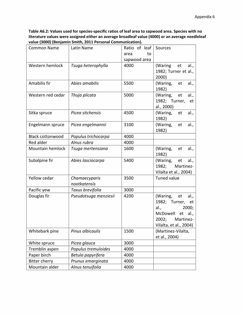
species sapling establishment rate, ability to endure low-light conditions, and sapwood to heartwood turnover rates. Species were assigned a shade tolerance as well as an average lifespan, vertical root distribution, and drought tolerance based upon descriptions in Burns et al. (1990) and Klinka et al. (2000). Wood density, fire resistance, and the ratio of crown area to stem diameter were derived from the FVS/FFE model (Crookston et al., 2005; Reinhardt et al., 2007). The specific leaf area, which relates the leaf surface area per gram of carbon in the leaf, was derived from reported literature values (Table A6.1). The ratio between leaf area to sapwood area was also derived from reported literature values (Table A6.2). 6.2 Climate scenarios and datasets 6.2.1. Historical climate Historical monthly weather station data was downloaded from the Environment Canada website (Environment Canada 2011). Seasonal climate indices were created from the data by excluding seasons with incomplete records (missing data or missing months). The Terrace meteorological record was created from the meteorological stations: Terrace A (1953 – 2010) and Terrace PCC (1968 – 2007). The Prince Rupert record is from three stations: Prince Rupert (1908 – 1962), Prince Rupert A (1962 – 2006) and Prince Rupert AWOS (2005 – 2007). The assembled record is an average between the stations for years with overlapping coverage, allowing for a more complete record. Small geographic differences between the neighbouring stations were assumed to be insignificant to the climate record (maximum horizontal distance between stations is approximately six kilometers with a vertical distance of 160 m). 6.2.2. Gridded climate for model runs The LPJ-GUESS model required climate inputs are mean monthly temperature, precipitation and cloud cover. Climate scenarios were selected following Spittlehouse and Murdock (2010). The three models/emissions scenarios are listed in Table 5.1 of Chapter 5. These model/emission scenarios effectively cover the climate space of the models of the Fourth Assessment of the Inter-governmental Panel on Climate Change (IPCC) (Meehl, et al., 2007) for B.C.

The three model/emission scenarios have been downscaled from their native general circulation model grids to a resolution of 30 arc seconds using the ClimateWNA software (Wang et al., 2011). Monthly climate data for the historical period (1906 – 2006) was downscaled similarly from the 0.5° resolution CRU-TS 3.0 dataset (CRU 2008). The future scenarios were available as an average year of monthly mean climate covering thirty years for the 2020s (2010-2039), 2050s (2040-69) and 2080s (2070-2099). A continuous monthly climatology was created by linear interpolation between these years for each month. Inter-annual variability was added to the future climate by addition of the historic variability from 1906 – 1980. The historical variability is calculated from each month’s deviation in climate relative to the mean (absolute for temperature, relative for precipitation and cloud cover) over the detrended historical period and adding that on to the future climate linear interpolation.

As the ClimateWNA program does not downscale cloud cover, we used the CRU-TS 3.1 cloud cover fields (CRU 2008) with linear interpolation to 30 arc seconds. We did not attempt in our downscaling of the cloud cover data to further account for topography due to lack of adequate data for evaluation. The two areas within the study region with extensive cloud cover records (Terrace and Prince Rupert) are both located in valley bottoms. We are not aware of any other stations at higher elevations.

Appendix 6

Table A6.1 caption: Specific leaf area (SLA) values for the nineteen parameterized tree species. SLA values are listed along with the literature source. When multiple sources existed the value was tuned to be within the range given and to give the best present day distribution.

Common Name Latin Name Specific Leaf Area (cm2 g-

1)

Sources

Western hemlock Tsuga heterophylla 21.0 (Kershaw et al., 1995; White et al., 2000; Mitchell, 2001; Duursma et al., 2005)

Amabilis fir Abies amabilis 13.5 (Mitchell, 2001)

Western red cedar Thuja plicata 10.6 (Duursma, et al., 2005)

Sitka spruce Picea sitchensis 15.0 (Gower et al., 1990; Townend, 1995)

Engelmann spruce Picea engelmannii 7.7 (Chen, 1997)

Black cottonwood Populus trichocarpa 24.5 (Sigurdsson et al., 2001) and for hybrids of P. trichocarpa and P. deltoides (Heilman et al., 1994)

Red alder Alnus rubra 23.0 (Chan et al., 2003)

Mountain hemlock Tsuga mertensiana 9.2 (White, et al., 2000)

Subalpine fir Abies lasciocarpa 7.6 (Klinka et al., 1992; Klinka, et al., 2000; Duursma, et al., 2005; Bansal et al., 2010)

Yellow cedar Chamaecyparis nootkatensis

10.0

Pacific yew Taxus brevifolia 17.0 (Mitchell, 2001) –average of sunlight and shaded values

Douglas fir Pseudotsuga menziesii 9.0 (Kershaw, et al., 1995; White, et al., 2000; Weiskittel et al., 2008)

Whitebark pine Pinus alibcaulis 8.9 (White, et al., 2000)

White spruce Picea glauca 7.0 (Klinka, et al., 1992; White, et al., 2000)

Tremblin aspen Populus tremuloides 24.2 (White, et al., 2000)

Paper birch Betula papyrifera 10.9 (Ashton et al., 1998)

Bitter cherry Prunus emarginata 33.5 Average of P. pensylvania and P. serotina in (White, et al., 2000)

Mountain alder Alnus tenuifolia 37.2 (Anderson et al., 2004)

Appendix 6

Table A6.2: Values used for species-specific ratios of leaf area to sapwood area. Species with no literature values were assigned either an average broadleaf value (4000) or an average needleleaf value (3000) (Benjamin Smith, 2011 Personal Communication).

Common Name Latin Name Ratio of leaf area to sapwood area

Sources

Western hemlock Tsuga heterophylla 4000 (Waring et al., 1982; Turner et al., 2000)

Amabilis fir Abies amabilis 5500 (Waring, et al., 1982)

Western red cedar Thuja plicata 5000 (Waring, et al., 1982; Turner, et al., 2000)

Sitka spruce Picea sitchensis 4500 (Waring, et al., 1982)

Engelmann spruce Picea engelmannii 3100 (Waring, et al., 1982)

Black cottonwood Populus trichocarpa 4000

Red alder Alnus rubra 4000

Mountain hemlock Tsuga mertensiana 1600 (Waring, et al., 1982)

Subalpine fir Abies lasciocarpa 5400 (Waring, et al., 1982; Martinez-Vilalta et al., 2004)

Yellow cedar Chamaecyparis nootkatensis

3500 Tuned value

Pacific yew Taxus brevifolia 3000

Douglas fir Pseudotsuga menziesii 4200 (Waring, et al., 1982; Turner, et al., 2000; McDowell et al., 2002; Martinez-Vilalta, et al., 2004)

Whitebark pine Pinus albicaulis 1500 (Martinez-Vilalta, et al., 2004)

White spruce Picea glauca 3000

Tremblin aspen Populus tremuloides 4000

Paper birch Betula papyrifera 4000

Bitter cherry Prunus emarginata 4000

Mountain alder Alnus tenuifolia 4000

Appendix 6

6.3. Carbon dioxide datasets

The historical annual CO2 concentration dataset from 1906 to 1958 is calculated from a spline fit to Antarctic firn air samples as described in Krumhardt & Kaplan (2010). The annual CO2 concentration for years 1959 to 2010 are from the NOAA Mauna Loa flask observations (Conway et al., 2011). Small differences in annual CO2 concentration between either, Antarctica or Mauna Loa and the study site were ignored. Future emission scenarios A1B, A2 and B1 were obtained for two carbon models (BernCC and ISAM) used in the 4th Assessment of the IPCC (Meehl, et al., 2007). The carbon model outputs for each emissions scenario are decadal means (IPCC, 2001) and were linearly interpolated to produce an annually resolved dataset suitable for input to LPJ-GUESS. 6.4. Soils textural datasets

The LPJ-GUESS model requires soil information in the form of a soil code following Prentice et al. (1992)(Table A6.3). The Harmonized World Soils Database (HWSD) version 1.1. is available at a resolution of 30 arc seconds (FAO/IIASA/ISRIC/ISSCAS/JRC, 2009). The variables of bulk density, clay fraction, and the USDA code for two different soil depths corresponding to the upper (0 – 0.3 m) and lower (0. 3 – 1.0 m) soil depths of LPJ-GUESS were extracted from the HWSD. The HWSD soil information was transferred to the LPJ-GUESS soil codes following the scheme in Table A6.3. The soil bulk density and clay fraction were used in the new soil heterotrophic parameterization (Appendix 6.1.2). Table A3 caption: Scheme to translate USDA soil textural code into corresponding LPJ-GUESS soil code (as defined in Prentice et al. (1992))

USDA soil textural code

LPJ-GUESS Soil Code

Soil Textural Description

1 1 Fine

2 5 Medium-coarse

3 1 Fine

4 5 Medium-coarse

5 7 Fine medium coarse

6 2 Medium

7 2 Medium

8 6 Fine-coarse

9 7 Fine medium coarse

10 6 Fine-coarse

11 5 Medium-coarse

12 3 Coarse

13 3 Coarse 6.5. Harvesting Scenarios Coast Tsimshian Resources harvests in an area much smaller than that CCAP study area, we limited our harvesting simulations to the same areal extent and in doing so were able to use the same data used provided by Cortex Consultants for the SRWCP study area (See Chapter 10 an Appendix 10.1). The Vegetation Resource Inventory (VRI) was used to determine the areal extent of historical harvesting in the SRWCP region (Ministry of Forests, 2011). VRI is available as a GIS dataset with polygons

Appendix 6

corresponding to cutblocks or management units. Importantly, the publically available VRI dataset does not include information for the lands under Tree Farm Licence 1 (TFL1), which makes up a significant portion of the SRWCP study area (See Figure 7.3). As we were not able to obtain information on past harvesting in TFL1, we have estimated harvesting using the following scheme. We used the history of TFL1’s areal extent and allowable annual cut (AAC) (Sutherland, 2008) to determine an annual cut (cubic meters of wood per year) normalized to TFL1’s present areal extent. The normalization accounts for changes in TFL1’s areal extent, with corresponding changes in AAC, through its history. We determined the areal extent that must be harvested each year, to fulfill the AAC, using yield tables (cubic meters of wood per hectare) for the main BEC zones of TFL1 (Coastal Western Hemlock, Mountain Hemlock, and Interior Cedar Hemlock). The available yield tables published for TFL1 are for stands of 30 -110 years of age (Sterling Wood Group Inc. 2004). Several assumptions were made using this approach. First, the timber harvested was only that allowed by the AAC with neither undercut nor overcut possible. Second, that the volume of harvestable wood per hectare can be well represented by the yield tables referenced. Third, market conditions did not influence the harvest of timber from that prescribed by the AAC. This final assumption is almost certainly incorrect in the last decade given the slowdown in harvesting evident in the non-TFL1 areas of the SRWCP (see Fig 6.4). For non-TFL1 regions included in the VRI database we used the original VRI values and simply aggregated the areal extent of polygons harvested in each year.

Future harvesting for the entire SRWCP region, including TFL1, was prescribed by the scenarios determined by Cortex model (See Chapter 10 and Appendix 10.1). As establishment in LPJ-GUESS was constrained to occur only every five years, we used the harvest date within the VRI and Cortex outputs, as well as our TFL1 estimates, to combine the annual harvesting into 5-year bins. Estimated harvesting areal extents per five-year bin are shown in Figure 6.4.

During years of harvest, we randomly distributed the prescribed amount of harvesting within the non-Alpine Tundra (AT) BEC units of the SRWCP area. Grid cells were harvested as clear cuts with no trees allowed remain after harvest in the grid cell. All fine root mass and 30% of the total sapwood and heartwood mass was passed to the soil carbon pools. The 30% represents coarse roots, tree limbs and wastage during harvest. The leaf mass of the tree was transferred to the litter carbon pool. The remaining 70% of the sapwood and heartwood is assumed to be transported off-site and to remain without further decomposition (thus no further C emissions can come from these wood products). Grid cells were not harvested twice within the same simulation, i.e. no harvesting of second growth timber permitted. After harvest, each grid cell was replanted within the same year. The replanting excluded species that were not explicitly planted for that establishment year. Following establishment years, natural regeneration was permitted on the harvested grid cells from non-planted species. The planted species were established at a stem density of 400 stems per hectare for three species: Western Red Cedar (Thuja plicata), Amabilis Fir (Abies amabilis), and Western Hemlock (Tsuga heterophylla), giving a total density of 1200 stems per hectare following practices in the region (Engelbertink, 2011 Personal Communication). These three species were planted in both historical and future harvesting and across all zones of the SRWCP region.

Appendix 6

6.6. Calibration of Projection Confidence Levels

Table A6.4: Calibration of confidence levels

Confidence Level Description

High Good agreement between all three-climate models/scenarios simulations. Direction and magnitude of change is reasonably consistent. For estimations based upon the scientific literature, studies are peer-reviewed, specific to the general region, and present convincing evidence supporting their claims.

Moderate Majority agreement of the climate models/scenarios simulations. Direction and magnitude of change is generally consistent. For estimations based upon the scientific literature, the studies are peer-reviewed, likely applicable to the study region being, and present convincing evidence supporting their claims.

Low Deviation between the climate models/scenarios simulations. Direction of change is generally consistent but magnitude of change is not consistent. For estimations based upon the scientific literature, the studies are peer-reviewed but there is little consensus in the literature. Trend estimation is based upon weight of evidence from recent studies of regions similar or the same as the study region.

Very Low Large deviation between the climate models/scenarios simulations. Direction and magnitude of change is generally inconsistent. For estimations based upon the scientific literature, the studies are peer-reviewed or are technical reports. There is no clear consensus in the literature or the studies are not easily applied to our study region.

None Uncertainties in the projection are too high to allow an estimate. There does not exist good agreement in studies in the scientific literature to draw from.

Appendix 6

Bibliography

Abeysirigunawardena, D. S., Gilleland, E., Bronaugh, D., & Wong, P. (2009). Extreme wind regime responses to climate variability and change in the inner south coast of British Columbia, Canada. Atmosphere-Ocean, 47(1), 41-62. doi: 10.3137/Ao1003.2009

Anderson, M. D., Ruess, R. W., Uliassi, D. D., & Mitchell, J. S. (2004). Estimating N-2 fixation in two species of Alnus in interior Alaska using acetylene reduction and N-15(2) uptake. Ecoscience, 11(1), 102-112.

Ashton, P. M. S., Olander, L. P., Berlyn, G. P., Thadani, R., & Cameron, I. R. (1998). Changes in leaf structure in relation to crown position and tree size of Betula papyrifera within fire-origin stands of interior cedar-hemlock. Canadian Journal of Botany-Revue Canadienne De Botanique, 76(7), 1180-1187.

Banner, A., MacKenzie, W., Haeussler, S., Thomson, S., Pojar, J., & Trowbridge, R. (1993). A field guide to site identification and interpretation for the Prince Rupert forest region. Victoria, B.C.: Crown Publications.

Bansal, S., & Germino, M. J. (2010). Variation in ecophysiological properties among conifers at an ecotonal boundary: comparison of establishing seedlings and established adults at timberline. Journal of Vegetation Science, 21(1), 133-142. doi: 10.1111/J.1654-1103.2009.01127.X

Beier, C. M., Sink, S. E., Hennon, P. E., D'Amore, D. V., & Juday, G. P. (2008). Twentieth-century warming and the dendroclimatology of declining yellow-cedar forests in southeastern Alaska. Canadian Journal of Forest Research-Revue Canadienne De Recherche Forestiere, 38(6), 1319-1334. doi: 10.1139/X07-240

Boateng, K. (2011). Spore dispersal and infection of Dothistroma septosporum in Northern British Columbia. M.Sc., University of Northern British Columbia, Prince George.

Bonsal, B. R., Zhang, X., Vincent, L. A., & Hogg, W. D. (2001). Characteristics of daily and extreme temperatures over Canada. Journal of Climate, 14(9), 1959-1976.

Burns, R. M., & Honkala, B. H. (1990). Silvics of North America: 1. Conifers; 2. Hardwoods. Washington, D.C., 1-1703.

Chan, S. S., Radosevich, S. R., & Grotta, A. T. (2003). Effects of contrasting light and soil moisture availability on the growth and biomass allocation of Douglas-fir and red alder. Canadian Journal of Forest Research-Revue Canadienne De Recherche Forestiere, 33(1), 106-117. doi: Doi 10.1139/X02-148

Chen, H. Y. H. (1997). Interspecific responses of planted seedlings to light availability in interior British Columbia: survival, growth, allometric patterns, and specific leaf area. Canadian Journal of Forest Research-Revue Canadienne De Recherche Forestiere, 27(9), 1383-1393.

Conway, T., Lang, P. M., & Masarie, K. A. (2011). Atmospheric carbon dioxide dry air mole fractions from the NOAA ESRL carbon cycle cooperative global air sampline network, 1968-2010. (Version: 2011-10-14). ftp://ftp.cmdl.noaa.gov/ccg/co2/flask/event/.

Crookston, N. L., & Dixon, G. E. (2005). The forest vegetation simulator: a review of its structure, content, and applications. Computers and Electronics in Agriculture, 49, 60-80.

Appendix 6

CRU (University of East Anglia Climatic Research Unit), Jones, P., & Harris, I. (2008). CRU Time Series (TS) high resolution gridded datasets, NCAS British Atmospheric Data Centre. Retrieved from http://badc.nerc.ac.uk/view/badc.nerc.ac.uk__ATOM__dataent_1256223773328276.

Daniels, L. D., & Gray, R. W. (2006). Disturbance regimes of coastal British Columbia. BC Journal of Ecosystems and Management, 7(2), 44-56.

Daniels, L. D., Maertens, T. B., Stan, A. B., McCloskey, S. P. J., Cochrane, J. D., & Gray, R. W. (2011). Direct and indirect impacts of climate change on forests: three case studies from British Columbia. Canadian Journal of Plant Pathology-Revue Canadienne De Phytopathologie, 33(2), 108-116. doi: 10.1080/07060661.2011.563906

Diffenbaugh, N. S., Pal, J. S., Trapp, R. J., & Giorgi, F. (2005). Fine-scale processes regulate the response of extreme events to global climate change. Proceedings of the National Academy of Sciences of the United States of America, 102(44), 15774-15778. doi: 10.1073/Pnas.0506042102

Duursma, R. A., Marshall, J. D., Nippert, J. B., Chambers, C. C., & Robinson, A. P. (2005). Estimating leaf-level parameters for ecosystem process models: a study in mixed conifer canopies on complex terrain. Tree Physiology, 25(11), 1347-1359.

Engelbertink, R. (2011). [Common replanting practices of the Skeena region ]. Personal communication

Environment Canada (2011). National Climate Data and Information Archive. Available from Environment Canada National Climate Data and Information Archive Retrieved October 15th, 2010, from Government of Canada http://www.climate.weatheroffice.gc.ca/Welcome_e.html

FAO/IIASA/ISRIC/ISSCAS/JRC. (2009). Harmonized World Soil Database. Rome, Italy and Laxenburg, Austria: FAO and IIASA.

Flato, G. M., Boer, G. J., Lee, W. G., McFarlane, N. A., Ramsden, D., Reader, M. C., & Weaver, A. J. (2000). The Canadian Centre for Climate Modelling and Analysis global coupled model and its climate. Climate Dynamics, 16(6), 451-467.

Gower, S. T., & Richards, J. H. (1990). Larches - deciduous conifers in an evergreen world. Bioscience, 40(11), 818-826.

Griffin, B. J., Kohfeld, K. E., Cooper, A. B., & Boenisch, G. (2010). Importance of location for describing typical and extreme wind speed behavior. Geophysical Research Letters, 37. doi: 10.1029/2010gl045052.

Heilman, P. E., & Xie, F. G. (1994). Effects of nitrogen-fertilization on leaf-area, light interception, and productivity of short-rotation Populus-Trichocarpa X Populus-Deltoides hybrids. Canadian Journal of Forest Research-Revue Canadienne De Recherche Forestiere, 24(1), 166-173.

Hennon, P. E., Shaw, C. G. I., & Hansen, E. M. (1992). Cedar decline: distribution, epidemiology, and etiology. In P. D. Manion & D. Lachance (Eds.), Forest decline concepts (pp. 108-122). St. Paul MN: American Phytopathological Society Press.

Hickler, T., Smith, B., Prentice, I. C., Mjofors, K., Miller, P., Arneth, A., & Sykes, M. T. (2008). CO2 fertilization in temperate FACE experiments not representative of boreal and tropical forests. Global Change Biology, 14(7), 1531-1542. doi: 10.1111/J.1365-2486.2008.01598.X

Appendix 6

IPCC. (2001). Climate change 2001: The scientific basis. Contributions of Working Group I to the Third Assessment Report of the Intergovernmental Panel on Climate Change. In J. T. Houghton, Y. Ding, D. J. Griggs, M. Noguer, P. J. v. d. Linden, X. Dai, K. Maskell & C. A. Johnson (Eds.), (pp. 881). Cambridge, U.K. and New York USA.

Jentsch, A., & Beierkuhnlein, C. (2008). Research frontiers in climate change: Effects of extreme meteorological events on ecosystems. Comptes Rendus Geoscience, 340(9-10), 621-628. doi: 10.1016/J.Crte.2008.07.002

Jobbagy, E. G., & Jackson, R. B. (2000). The vertical distribution of soil organic carbon and its relation to climate and vegetation. Ecological Applications, 10(2), 423-436.

Kershaw, J. A., & Maguire, D. A. (1995). Crown structure in western hemlock, douglas-fir, and grand fir in western Washington: Trends in branch-level mass and leaf area. Canadian Journal of Forest Research-Revue Canadienne De Recherche Forestiere, 25(12), 1897-1912.

Klinka, K., Wang, Q., Kayahara, G. J., Carter, R. E., & Blackwell, B. A. (1992). Light-growth response relationships in pacific silver fir (Abies amabilis) and sub-alpine fir (Abies lasiocarpa). Canadian Journal of Botany-Revue Canadienne De Botanique, 70(10), 1919-1930.

Klinka, K., Worrall, J., Skoda, L., & Varga, P. (2000). The distribution and synopsis of ecological and silvical characteristics of tree species of British Columbia's forests. Coquitlam, B.C.: Canadian Cartographics Ltd.

Krumhardt, K. M., & Kaplan, J. O. (2010). A spline fit to atmospheric CO2 records from Antarctic ice cores and measured concentrations for the last 25,000 years. ARVE Technical Report #2. École Polytechnique Fédérale de Lausanne. Lausanne. Retrieved from http://ecospriv4.epfl.ch/pub/ARVE_tech_report2_co2spline.pdf

Kurz, W. A., Dymond, C. C., Stinson, G., Rampley, G. J., Neilson, E. T., Carroll, A. L., . . . Safranyik, L. (2008). Mountain pine beetle and forest carbon feedback to climate change. Nature, 452(7190), 987-990. doi: 10.1038/Nature06777

Leung, L. R., Qian, Y., Bian, X. D., Washington, W. M., Han, J. G., & Roads, J. O. (2004). Mid-century ensemble regional climate change scenarios for the western United States. Climatic Change, 62(1-3), 75-113.

Manning, M. R., Edmonds, J., Emori, S., Grubler, A., Hibbard, K., Joos, F., . . . van Vuuren, D. P. (2010). Misrepresentation of the IPCC CO2 emission scenarios. Nature Geoscience, 3(6), 376-377.

Martinez-Vilalta, J., Sala, A., & Pinol, J. (2004). The hydraulic architecture of Pinaceae - a review. Plant Ecology, 171(1-2), 3-13.

McDowell, N., Barnard, H., Bond, B. J., Hinckley, T., Hubbard, R. M., Ishii, H., . . . Whitehead, D. (2002). The relationship between tree height and leaf area: sapwood area ratio. Oecologia, 132, 12-20. doi: 10.1007/s00442-002-0904-x

Meehl, G. A., & Stocker, T. F., W.D. Collins, P. Friedlingstein, A.T. Gaye, J.M. Gregory, A. Kitoh, R. Knutti, J.M. Murphy, A. Noda, S.C.B. Raper, I.G. Watterson, A.J. Weaver, Z.-C. Zhao (Eds.). (2007). Global Climate Projections. Cambridge, United Kingdom and New York, USA: Cambridge University Press.

Ministry of Forests, Lands, and Natural Resource Operations. (2011). Vegetation Resource Inventory. Victoria, B.C.: Province of British Columbia Retrieved from http://geobc.gov.bc.ca/.

Appendix 6

Mitchell, A. K. (2001). Growth limitations for conifer regeneration under alternative silvicultural systems in a coastal montane forest in British Columbia, Canada. Forest Ecology and Management, 145(1-2), 129-136.

Nakicenovic, N., Alcamo, J., Davis, G., Vries, B. d., Fenhann, J., Gaffin, S., . . . Dadi, Z. (Eds.). (2000). IPCC Special Report on Emissions Scenarios. Cambridge, UK: Cambridge University Press.

Peterson, T. C., Zhang, X. B., Brunet-India, M., & Vazquez-Aguirre, J. L. (2008). Changes in North American extremes derived from daily weather data. Journal of Geophysical Research-Atmospheres, 113(D7). doi: 10.1029/2007jd009453

Post, W. M., Emanuel, W. R., Zinke, P. J., & Stangenberger, A. G. (1982). Soil carbon pools and world life zones. Nature, 298(5870), 156-159.

Prentice, I. C., Cramer, W., Harrison, S. P., Leemans, R., Monserud, R. A., & Solomon, A. M. (1992). A global biome model based on plant physiology and dominance, soil properties and climate. Journal of Biogeography, 19(2), 117-134.

Reinhardt, E. D., & Crookston, N. L. (2007). The fire and fuels extension to the Forest Vegetation Simlator. Ogden, UT, USA.

Septer, D. (2007). Flooding and landslide events Northern British Columbia 1820 - 2006. Victora, BC: Province of British Columbia.

Sigurdsson, B. D., Thorgeirsson, H., & Linder, S. (2001). Growth and dry-matter partitioning of young Populus trichocarpa in response to carbon dioxide concentration and mineral nutrient availability. Tree Physiology, 21(12-13), 941-950.

Sitch, S., Smith, B., Prentice, C. I., Arneth, A., Bondeau, A., Cramer, W., . . . Venevsky, S. (2003 ). Evaluation of ecosystem dynamics, plant geography and terrestrial carbon cycling in the LPJ dynamic global vegetation model. Global Change Biology, 9, 161-185.

Smith, B. (2011). [Species parameters for use in the LPJ family of models]. Personal communication

Smith, B., Prentice, I. C., & Sykes, M. T. (2001). Representation of vegetation dynamics in the modelling of terrestrial ecosystems: comparing two contrasting approaches within European climate space. Global Ecology and Biogeography, 10(6), 621-637.

Spittlehouse, D., & Murdock, T. (2010). Choosing and applying climate change scenarios. Draft. FFESC Project 014. Victoria, B.C.

Sterling Wood Group Inc. (2004). TFL1 Vegetation Resources Inventory Attribute Adjustment (pp. 6). Victoria, B.C.

Sutherland, C. (2008). Tree Farm Licence 1. Coast Tsimshian Resources Limited Partnership. Rationale for allowable annual cut (AAC) determination (pp. 40). Victoria B.C.: Ministry of Forests.

Sutherland, J. (2010). Re-designation of Emergency Management Units. Victoria, B.C.: Retrieved from http://www.for.gov.bc.ca/ftp/HFP/external/!publish/EBBMA/EBBMA_2010/EBBMA MPB Memo June 10 2010.pdf.

Taylor, S. (2010). Pacific forestry centre pest outbreak dataset. Victoria, B.C.: Canadian Forestry Service.

Townend, J. (1995). Effects of elevated CO2, water and nutrients on Picea sitchensis (Bong) Carr seedlings. New Phytologist, 130(2), 193-206.

Appendix 6

Turner, D. P., Acker, S. A., Means, J. E., & Garman, S. L. (2000). Assessing alternative allometric algorithms for estimating leaf area of douglas-fir trees and stands. Forest Ecology and Management, 126(1), 61-76.

Wang, T., Hamann, A., Spittlehouse, D., & Murdock, T. (2011). ClimateWNA - High resolution spatial climate data for Western North America. Journal of Applied Meteorology and Climatology. doi: 10.1175/JAMC-D-11-043.1

Wang, T., Hamann, A., Spittlehouse, D. L., & Aitken, S. N. (2006). Development of scale-free climate data for western Canada for use in resource management. International Journal of Climatology, 26(3), 383-397.

Waring, R. H., Schroeder, P. E., & Oren, R. (1982). Application of the pipe model-theory to predict canopy leaf-area. Canadian Journal of Forest Research-Revue Canadienne De Recherche Forestiere, 12(3), 556-560.

Weiskittel, A. R., Temesgen, H., Wilson, D. S., & Maguire, D. A. (2008). Sources of within- and between-stand variability in specific leaf area of three ecologically distinct conifer species. Annals of Forest Science, 65(1). doi: 10.1051/Forest:2007075

White, M. A., Thornton, P., Running, S. W., & Nemani, R. R. (2000). Parameterization and sensitivity analysis of the BIOME-BGC terrestrial ecosystem model: Net primary production controls. Earth Interactions, 4(3), 1-85.

Woods, A., Coates, K. D., & Hamann, A. (2005). Is an unprecedented dothistroma needle blight epidemic related to climate change? Bioscience, 55(9), 761-769.

Woods, A. J., Heppner, D., Kope, H. H., Burleigh, J., & Maclauchlan, L. (2010). Forest health and climate change: A British Columbia perspective. Forestry Chronicle, 86(4), 412-422.

Yole, D., Lewis, T., Inselberg, A., Pojar, J., & Holmes, D. (1989). A field guide for identification and interpretation of the Engelmann Spruce- Subalpine Fir zone in the Prince Rupert forest region British Columbia. (17). Victoria,B C: Crown Publications.

Zhu, K., Woodall, C. W., & Clark, J. S. (2011). Failure to migrate: lack of tree range expansion in response to climate change. Global Change Biology. doi: 10.1111/j.1365-2486.2011.02571.x