272 CHAPTER 5: CENSUSES FROM THE SKY 5.1. Population as a Dependent Variable from Urban Areas After dasymetric densities had been calculated (Tables 98 to 124) and spatially represented in Chapter 4, the same information about demographic data and urbanized surfaces is used to know the degree in which urban areas are predicting population statistics through a chronological series of linear regressions for the 110 census tracts, where population becomes the dependent variable (Y) of urban areas (X). The dependent or response variable Y (population) in a linear regression equation is modeled by a least squares function of the independent or explanatory variable X (Urban areas) (Sirkin 2006). This function is a linear combination of two model parameters or regression coefficients: a (Y-intercept: the value of Y when X = 0) and b (slope of the regression line) and an error term, which is treated as a random variable and it represents the unexplained variation in the dependent variable (Rogerson 2006). The input data for this linear regression model consist of two kinds of data: first, the count of the number of urbanized pixels in every census tract obtained from urban land cover through satellite image classification or SLEUTH simulation (spatial independent variable X); and second, the statistics about population for every census tract obtained from censuses (Geolytics) and estimated or projected from known values (statistical dependent variable Y). The regression formula for this specific case is the following one: Y = a + b * X has been replaced by: P act = a + b * A Where: P act is the number of actual population (dependent variable: Y) a is a constant (a regression coefficient) and represents the y-intercept: the value of y when x =0. _ _ _ _ a = Y – b * X has been replaced by: a = P act – b * A b is a constant (a regression coefficient) and represents the slope of the regression line. ( ) ( ) ( ) ∑ ∑ ∑ ∑ - - = n X X n Y X XY b 2 2 has been replaced by: ( ) ( ) ( ) ∑ ∑ ∑ ∑ ∑ - - = n A A n Pact A Pact A b 2 2 * A is the number of urbanized pixels (independent variable: X). A or Area is the result of counting just the urbanized pixels (through the use of a binary mask) in every census tract from the land cover data derived from satellite image classification or from the SLEUTH simulation.

Welcome message from author
This document is posted to help you gain knowledge. Please leave a comment to let me know what you think about it! Share it to your friends and learn new things together.
Transcript
272
CHAPTER 5: CENSUSES FROM THE SKY
5.1. Population as a Dependent Variable from Urban Areas
After dasymetric densities had been calculated (Tables 98 to 124) and spatially represented in
Chapter 4, the same information about demographic data and urbanized surfaces is used to know
the degree in which urban areas are predicting population statistics through a chronological
series of linear regressions for the 110 census tracts, where population becomes the dependent
variable (Y) of urban areas (X).
The dependent or response variable Y (population) in a linear regression equation is modeled
by a least squares function of the independent or explanatory variable X (Urban areas) (Sirkin
2006). This function is a linear combination of two model parameters or regression coefficients:
a (Y-intercept: the value of Y when X = 0) and b (slope of the regression line) and an error term,
which is treated as a random variable and it represents the unexplained variation in the dependent
variable (Rogerson 2006).
The input data for this linear regression model consist of two kinds of data: first, the count of
the number of urbanized pixels in every census tract obtained from urban land cover through
satellite image classification or SLEUTH simulation (spatial independent variable X); and
second, the statistics about population for every census tract obtained from censuses (Geolytics)
and estimated or projected from known values (statistical dependent variable Y). The regression
formula for this specific case is the following one:
Y = a + b * X has been replaced by: Pact = a + b * A
Where:
Pact is the number of actual population (dependent variable: Y)
a is a constant (a regression coefficient) and represents the y-intercept: the value of y when x =0.
_ _ _ _
a = Y – b * X has been replaced by: a = Pact – b * A
b is a constant (a regression coefficient) and represents the slope of the regression line.
( )( )
( )∑
∑∑∑
−
−=
n
XX
n
YXXY
b2
2
has been replaced by:
( )( )
( )∑ ∑
∑∑∑
−
−=
n
AA
n
PactAPactA
b2
2
*
A is the number of urbanized pixels (independent variable: X). A or Area is the result of
counting just the urbanized pixels (through the use of a binary mask) in every census tract from
the land cover data derived from satellite image classification or from the SLEUTH simulation.
273
After the linear equation is generated using SPSS software, the following results are
produced:
Pearson Correlation Coefficient (R) is a common measure between two variables X and Y that
reflects the degree of linear relationship between them, ranging from +1 (a perfect positive linear
relationship between variables) to -1 (a perfect negative linear relationship between variables),
while a correlation of 0 means there is no linear relationship between the two variables. In
practice, these values are rarely if ever 0, 1, or -1 (Rogerson 2006). Because correlation does not
imply causation, a high correlation between two variables does not represent enough evidence
that changes in one variable will generate changes in the other variable.
Coefficient of Determination (R2) is the square of the correlation coefficient between the
constructed predictor X and the response variable Y (Sirkin 2006). This statistical measure
indicates the degree in which the regression line approximates the real data points, being a R2 of
1.0 the regression line that perfectly fits the data, explaining all the variability in Y, while R2 = 0
indicates no linear relationship between the independent variable X with its dependent variable
Y.
Adjusted Coefficient of Determination (Adjusted R2) adjusts for the unbiased variances of the
errors and of the observations in a model and unlike R2, this index increases only if the new
values improve the model more than would be expected by chance (Sirkin 2006). The adjusted
R2 can be negative, and will always be less than or equal to R
2.
Standard Errors of the Coefficients are the estimated standard deviations of the differences
(errors) in the regression for coefficients a and b (Rogerson 2006). It results from the standard
deviation of the individual differences or individual errors between the values and the regression
line and therefore, it is a measure of the precision with which the regression coefficients are
measured.
t tests results from dividing the values of constants a and b by their respective standard errors
(standard deviations) and they are used to assess if the null hypothesis (H0) is true or not. A null
hypothesis (H0) is a scenario set up to be nullified or statistically refuted if observations are the
result of chance (Rogerson 2006).
F test consists on the square of the t-test for the b coefficient and it is used to evaluate the
significance of the regression model as a whole, in other words, to test the significance of R and
therefore R2 as well (Rogerson 2006).
P values are used to assess the t tests of a and b coefficients. The P value of b is the same
value than the P value for the F test (square of t test for b). These values are the result of the
software comparison between the t statistics on the variables with the values in the distribution
(Rogerson 2006). P values are used with a degree of confidence, usually higher than 95% to
reject the null hypothesis, in other words that the data (in this case, the dependent variable
population) does not result from chance. If P value or Probability (F) < 0.05, the model is
considered significantly better than would be expected by chance alone and it is possible to reject
274
the null hypothesis (Sirkin 2006), confirming in the other hand the dependency of a linear
relationship of Y (Population) from X (Urban Areas).
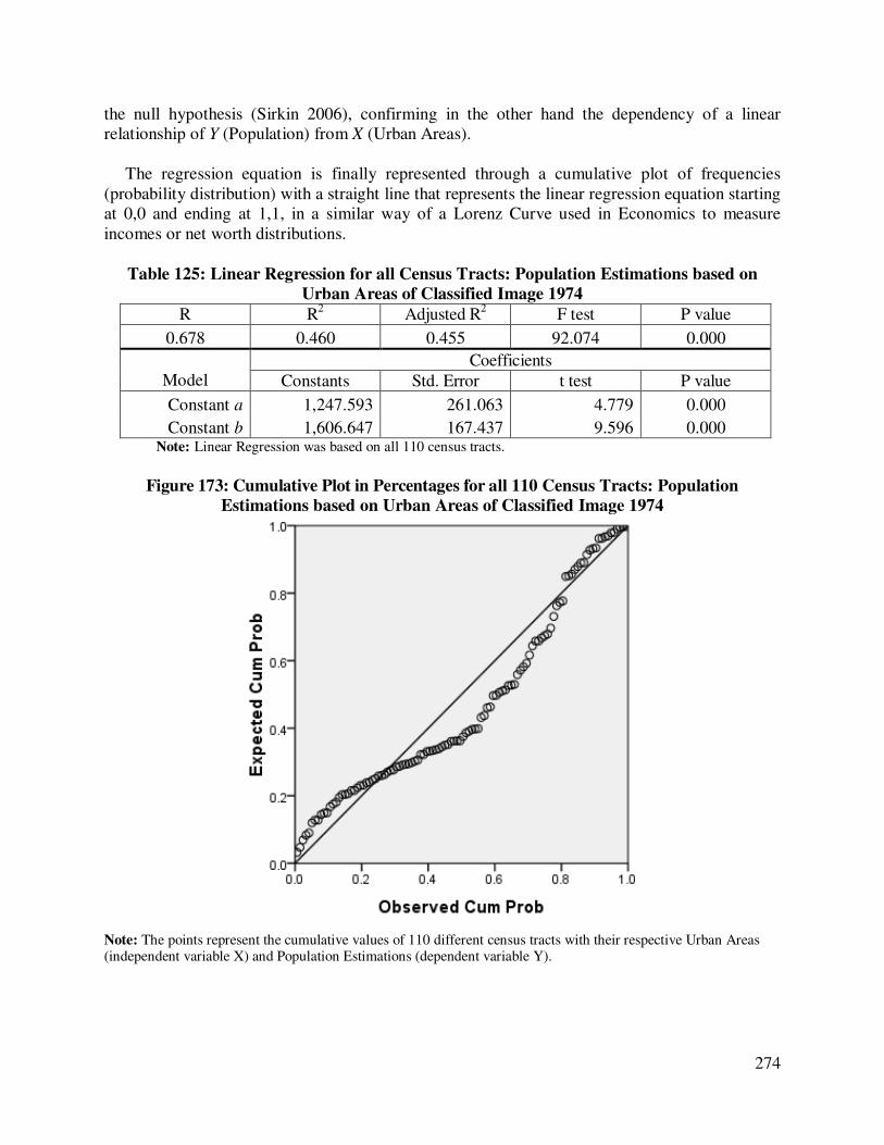
The regression equation is finally represented through a cumulative plot of frequencies
(probability distribution) with a straight line that represents the linear regression equation starting
at 0,0 and ending at 1,1, in a similar way of a Lorenz Curve used in Economics to measure
incomes or net worth distributions.
Table 125: Linear Regression for all Census Tracts: Population Estimations based on
Urban Areas of Classified Image 1974
R R2 Adjusted R
2 F test P value
0.678 0.460 0.455 92.074 0.000
Model
Coefficients
Constants Std. Error t test P value
Constant a 1,247.593 261.063 4.779 0.000
Constant b
1,606.647 167.437 9.596 0.000 Note: Linear Regression was based on all 110 census tracts.
Figure 173: Cumulative Plot in Percentages for all 110 Census Tracts: Population
Estimations based on Urban Areas of Classified Image 1974
Note: The points represent the cumulative values of 110 different census tracts with their respective Urban Areas (independent variable X) and Population Estimations (dependent variable Y).

275
Table 126: Linear Regression for all Census Tracts: Population Estimations based on
Urban Areas of Simulation 1975
R R2 Adjusted R
2 F test P value
0.694 0.481 0.476 100.154 0.000
Model
Coefficients
Constants Std. Error t test P value
Constant a 1,216.344 251.701 4.833 0.000
Constant b
1,585.500
158.428 10.008 0.000 Note: Linear Regression was based on all 110 census tracts.
Figure 174: Cumulative Plot in Percentages for all 110 Census Tracts: Population
Estimations based on Urban Areas of Simulation 1975
Note: The points represent the cumulative values of 110 different census tracts with their respective Urban Areas (independent variable X) and Population Estimations (dependent variable Y).
276
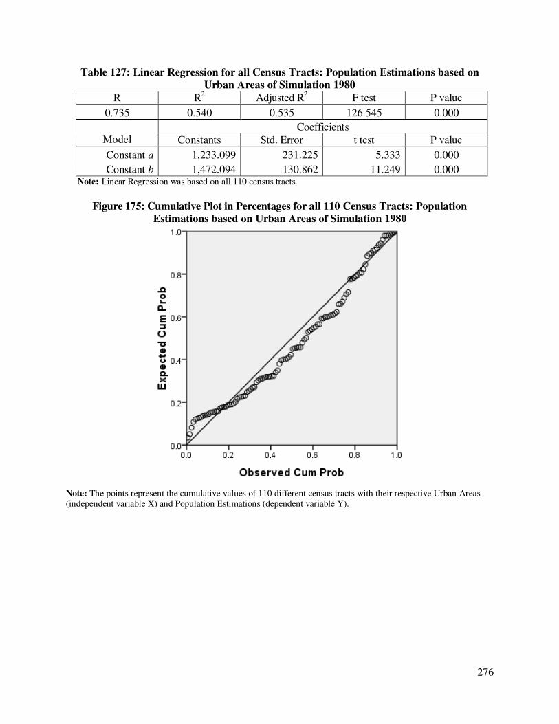
Table 127: Linear Regression for all Census Tracts: Population Estimations based on
Urban Areas of Simulation 1980
R R2 Adjusted R
2 F test P value
0.735 0.540 0.535 126.545 0.000
Model
Coefficients
Constants Std. Error t test P value
Constant a 1,233.099 231.225 5.333 0.000
Constant b
1,472.094 130.862 11.249 0.000 Note: Linear Regression was based on all 110 census tracts.
Figure 175: Cumulative Plot in Percentages for all 110 Census Tracts: Population
Estimations based on Urban Areas of Simulation 1980
Note: The points represent the cumulative values of 110 different census tracts with their respective Urban Areas (independent variable X) and Population Estimations (dependent variable Y).

277
Table 128: Linear Regression for all Census Tracts: Population Estimations based on
Urban Areas of Simulation 1985
R R2 Adjusted R
2 F test P value
0.725 0.526 0.521 119.778 0.000
Model
Coefficients
Constants Std. Error t test P value
Constant a 1,674.716 246.871 6.784 0.000
Constant b
1,388.872 126.903 10.944 0.000 Note: Linear Regression was based on all 110 census tracts.
Figure 176: Cumulative Plot in Percentages for all 110 Census Tracts: Population
Estimations based on Urban Areas of Simulation 1980
Note: The points represent the cumulative values of 110 different census tracts with their respective Urban Areas (independent variable X) and Population Estimations (dependent variable Y).

278
Table 129: Linear Regression for all Census Tracts: Population Estimations based on
Urban Areas of Classified Image 1986
R R2 Adjusted R
2 F test P value
0.711 0.506 0.502 110.696 0.000
Model
Coefficients
Constants Std. Error t test P value
Constant a 1,631.828 268.739 6.072 0.000
Constant b
1,453.181 138.119 10.521 0.000 Note: Linear Regression was based on all 110 census tracts.
Figure 177: Cumulative Plot in Percentages for all 110 Census Tracts: Population
Estimations based on Urban Areas of Classified Image 1986
Note: The points represent the cumulative values of 110 different census tracts with their respective Urban Areas (independent variable X) and Population Estimations (dependent variable Y).

279
Table 130: Linear Regression for all Census Tracts: Population Estimations based on
Urban Areas of Simulation 1986
R R2 Adjusted R
2 F test P value
0.715 0.512 0.507 113.174 0.000
Model
Coefficients
Constants Std. Error t test P value
Constant a 1,765.188 254.711 6.930 0.000
Constant b
1,367.089 128.506 10.638 0.000 Note: Linear Regression was based on all 110 census tracts.
Figure 178: Cumulative Plot in Percentages for all 110 Census Tracts: Population
Estimations based on Urban Areas of Simulation 1986
Note: The points represent the cumulative values of 110 different census tracts with their respective Urban Areas (independent variable X) and Population Estimations (dependent variable Y).

280
Table 131: Linear Regression for all Census Tracts: Population Estimations based on
Urban Areas of Simulation 1990
R R2 Adjusted R
2 F test P value
0.644 0.415 0.410 76.698 0.000
Model
Coefficients
Constants Std. Error t test P value
Constant a 2,041.217 303.813 6.719 0.000
Constant b
1,245.428 142.209 8.758 0.000 Note: Linear Regression was based on all 110 census tracts.
Figure 179: Cumulative Plot in Percentages for all 110 Census Tracts: Population
Estimations based on Urban Areas of Simulation 1990
Note: The points represent the cumulative values of 110 different census tracts with their respective Urban Areas (independent variable X) and Population Estimations (dependent variable Y).

281
Table 132: Linear Regression for all Census Tracts: Population Estimations based on
Urban Areas of Classified Image 1992
R R2 Adjusted R
2 F test P value
0.720 0.518 0.514 116.191 0.000
Model
Coefficients
Constants Std. Error t test P value
Constant a 1,638.064 297.163 5.512 0.000
Constant b
1,474.131 136.757 10.779 0.000 Note: Linear Regression was based on all 110 census tracts.
Figure 180: Cumulative Plot in Percentages for all 110 Census Tracts: Population
Estimations based on Urban Areas of Classified Image 1992
Note: The points represent the cumulative values of 110 different census tracts with their respective Urban Areas (independent variable X) and Population Estimations (dependent variable Y).

282
Table 133: Linear Regression for all Census Tracts: Population Estimations based on
Urban Areas of Simulation 1992
R R2 Adjusted R
2 F test P value
0.625 0.390 0.384 69.084 0.000
Model
Coefficients
Constants Std. Error t test P value
Constant a 2,133.334 322.400 6.617 0.000
Constant b
1,207.079 145.227 8.312 0.000 Note: Linear Regression was based on all 110 census tracts.
Figure 181: Cumulative Plot in Percentages for all 110 Census Tracts: Population
Estimations based on Urban Areas of Simulation 1992
Note: The points represent the cumulative values of 110 different census tracts with their respective Urban Areas
(independent variable X) and Population Estimations (dependent variable Y).

283
Table 134: Linear Regression for all Census Tracts: Population Estimations based on
Urban Areas of Simulation 1995
R R2 Adjusted R
2 F test P value
0.586 0.344 0.338 56.610 0.000
Model
Coefficients
Constants Std. Error t test P value
Constant a 2,282.960 373.546 6.112 0.000
Constant b
1,196.608 159.040 7.524 0.000 Note: Linear Regression was based on all 110 census tracts.
Figure 182: Cumulative Plot in Percentages for all 110 Census Tracts: Population
Estimations based on Urban Areas of Simulation 1995
Note: The points represent the cumulative values of 110 different census tracts with their respective Urban Areas (independent variable X) and Population Estimations (dependent variable Y).

284
Table 135: Linear Regression for all Census Tracts: Population Estimations based on
Urban Areas of Simulation 2000
R R2 Adjusted R
2 F test P value
0.480 0.230 0.223 32.308 0.000
Model
Coefficients
Constants Std. Error t test P value
Constant a 2,609.113 522.806 4.991 0.000
Constant b
1,156.815 203.520 5.684 0.000 Note: Linear Regression was based on all 110 census tracts.
Figure 183: Cumulative Plot in Percentages for all 110 Census Tracts: Population
Estimations based on Urban Areas of Simulation 2000
Note: The points represent the cumulative values of 110 different census tracts with their respective Urban Areas (independent variable X) and Population Estimations (dependent variable Y).

285
Table 136: Linear Regression for all Census Tracts: Population Estimations based on
Urban Areas of Classified Image 2001
R R2 Adjusted R
2 F test P value
0.778 0.606 0.602 165.823 0.000
Model
Coefficients
Constants Std. Error t test P value
Constant a 1,829.951 321.167 5.698 0.000
Constant b
1,530.358 118.842 12.877 0.000 Note: Linear Regression was based on all 110 census tracts.
Figure 184: Cumulative Plot in Percentages for all 110 Census Tracts: Population
Estimations based on Urban Areas of Classified Image 2001
Note: The points represent the cumulative values of 110 different census tracts with their respective Urban Areas (independent variable X) and Population Estimations (dependent variable Y).

286
Table 137: Linear Regression for all Census Tracts: Population Estimations based on
Urban Areas of Simulation 2001
R R2 Adjusted R
2 F test P value
0.471 0.221 0.214 30.712 0.000
Model
Coefficients
Constants Std. Error t test P value
Constant a 2,650.267 544.040 4.871 0.000
Constant b
1,153.768 208.191 5.542 0.000 Note: Linear Regression was based on all 110 census tracts.
Figure 185: Cumulative Plot in Percentages for all 110 Census Tracts: Population
Estimations based on Urban Areas of Simulation 2001
Note: The points represent the cumulative values of 110 different census tracts with their respective Urban Areas (independent variable X) and Population Estimations (dependent variable Y).

287
Table 138: Linear Regression for all Census Tracts: Population Estimations based on
Urban Areas of Simulation 2005 smart
R R2 Adjusted R
2 F test P value
0.784 0.614 0.611 171.931 0.000
Model
Coefficients
Constants Std. Error t test P value
Constant a 1,651.244 362.216 4.559 0.000
Constant b
1,714.811 130.779 13.112 0.000 Note: Linear Regression was based on all 110 census tracts.
Figure 186: Cumulative Plot in Percentages for all 110 Census Tracts: Population
Estimations based on Urban Areas of Simulation 2005 smart
Note: The points represent the cumulative values of 110 different census tracts with their respective Urban Areas (independent variable X) and Population Estimations (dependent variable Y).

288
Table 139: Linear Regression for all Census Tracts: Population Estimations based on
Urban Areas of Simulation 2005 normal
R R2 Adjusted R
2 F test P value
0.790 0.623 0.620 178.797 0.000
Model
Coefficients
Constants Std. Error t test P value
Constant a 1,638.082 356.746 4.592 0.000
Constant b
1,652.384 123.575 13.371 0.000 Note: Linear Regression was based on all 110 census tracts.
Figure 187: Cumulative Plot in Percentages for all 110 Census Tracts: Population
Estimations based on Urban Areas of Simulation 2005 normal
Note: The points represent the cumulative values of 110 different census tracts with their respective Urban Areas (independent variable X) and Population Estimations (dependent variable Y).

289
Table 140: Linear Regression for all Census Tracts: Population Estimations based on
Urban Areas of Simulation 2005 sprawl
R R2 Adjusted R
2 F test P value
0.789 0.623 0.620 178.599 0.000
Model
Coefficients
Constants Std. Error t test P value
Constant a 1,645.441 356.453 4.616 0.000
Constant b
1,598.262 119.594 13.364 0.000 Note: Linear Regression was based on all 110 census tracts.
Figure 188: Cumulative Plot in Percentages for all 110 Census Tracts: Population
Estimations based on Urban Areas of Simulation 2005 sprawl
Note: The points represent the cumulative values of 110 different census tracts with their respective Urban Areas (independent variable X) and Population Estimations (dependent variable Y).

290
Table 141: Linear Regression for all Census Tracts: Population Estimations based on
Urban Areas of Simulation 2010 smart
R R2 Adjusted R
2 F test P value
0.787 0.619 0.615 175.173 0.000
Model
Coefficients
Constants Std. Error t test P value
Constant a 1,342.928 435.958 3.080 0.003
Constant b
2,060.668 155.695 13.235 0.000 Note: Linear Regression was based on all 110 census tracts.
Figure 189: Cumulative Plot in Percentages for all 110 Census Tracts: Population
Estimations based on Urban Areas of Simulation 2010 smart
Note: The points represent the cumulative values of 110 different census tracts with their respective Urban Areas (independent variable X) and Population Estimations (dependent variable Y).

291
Table 142: Linear Regression for all Census Tracts: Population Estimations based on
Urban Areas of Simulation 2010 normal.
R R2 Adjusted R
2 F test P value
0.800 0.640 0.636 191.623 0.000
Model
Coefficients
Constants Std. Error t test P value
Constant a 1,306.950 420.922 3.105 0.002
Constant b
1,868.497 134.980 13.843 0.000 Note: Linear Regression was based on all 110 census tracts.
Figure 190: Cumulative Plot in Percentages for all 110 Census Tracts: Population
Estimations based on Urban Areas of Simulation 2010 normal
Note: The points represent the cumulative values of 110 different census tracts with their respective Urban Areas (independent variable X) and Population Estimations (dependent variable Y).
292
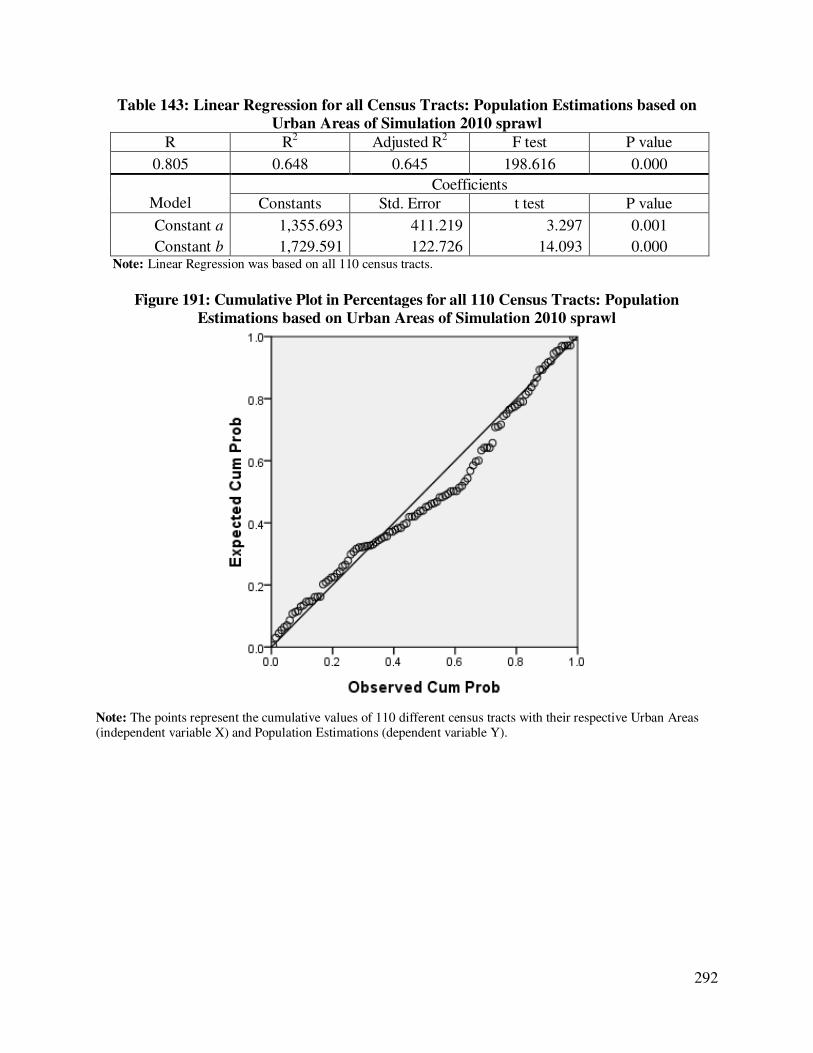
Table 143: Linear Regression for all Census Tracts: Population Estimations based on
Urban Areas of Simulation 2010 sprawl
R R2 Adjusted R
2 F test P value
0.805 0.648 0.645 198.616 0.000
Model
Coefficients
Constants Std. Error t test P value
Constant a 1,355.693 411.219 3.297 0.001
Constant b
1,729.591 122.726 14.093 0.000 Note: Linear Regression was based on all 110 census tracts.
Figure 191: Cumulative Plot in Percentages for all 110 Census Tracts: Population
Estimations based on Urban Areas of Simulation 2010 sprawl
Note: The points represent the cumulative values of 110 different census tracts with their respective Urban Areas (independent variable X) and Population Estimations (dependent variable Y).

293
Table 144: Linear Regression for all Census Tracts: Population Estimations based on
Urban Areas of Simulation 2015 smart
R R2 Adjusted R
2 F test P value
0.784 0.614 0.611 172.142 0.000
Model
Coefficients
Constants Std. Error t test P value
Constant a 961.884 516.867 1.861 0.065
Constant b
2,394.927 182.536 13.120 0.000 Note: Linear Regression was based on all 110 census tracts.
Figure 192: Cumulative Plot in Percentages for all 110 Census Tracts: Population
Estimations based on Urban Areas of Simulation 2015 smart
Note: The points represent the cumulative values of 110 different census tracts with their respective Urban Areas (independent variable X) and Population Estimations (dependent variable Y).

294
Table 145: Linear Regression for all Census Tracts: Population Estimations based on
Urban Areas of Simulation 2015 normal
R R2 Adjusted R
2 F test P value
0.807 0.652 0.648 201.918 0.000
Model
Coefficients
Constants Std. Error t test P value
Constant a 912.625 484.018 1.886 0.062
Constant b
2,049.709 144.246 14.210 0.000 Note: Linear Regression was based on all 110 census tracts.
Figure 193: Cumulative Plot in Percentages for all 110 Census Tracts: Population
Estimations based on Urban Areas of Simulation 2015 normal
Note: The points represent the cumulative values of 110 different census tracts with their respective Urban Areas (independent variable X) and Population Estimations (dependent variable Y).

295
Table 146: Linear Regression for all Census Tracts: Population Estimations based on
Urban Areas of Simulation 2015 sprawl
R R2 Adjusted R
2 F test P value
0.813 0.661 0.658 210.982 0.000
Model
Coefficients
Constants Std. Error t test P value
Constant a 990.197 469.972 2.107 0.037
Constant b
1,826.548 125.750 14.525 0.000 Note: Linear Regression was based on all 110 census tracts.
Figure 194: Cumulative Plot in Percentages for all 110 Census Tracts: Population
Estimations based on Urban Areas of Simulation 2015 sprawl
Note: The points represent the cumulative values of 110 different census tracts with their respective Urban Areas (independent variable X) and Population Estimations (dependent variable Y).

296
Table 147: Linear Regression for all Census Tracts: Population Estimations based on
Urban Areas of Simulation 2020 smart
R R2 Adjusted R
2 F test P value
0.782 0.611 0.607 169.466 0.000
Model
Coefficients
Constants Std. Error t test P value
Constant a 494.847 603.342 0.820 0.414
Constant b
2,740.155 210.491 13.018 0.000 Note: Linear Regression was based on all 110 census tracts.
Figure 195: Cumulative Plot in Percentages for all 110 Census Tracts: Population
Estimations based on Urban Areas of Simulation 2020 smart
Note: The points represent the cumulative values of 110 different census tracts with their respective Urban Areas (independent variable X) and Population Estimations (dependent variable Y).

297
Table 148: Linear Regression for all Census Tracts: Population Estimations based on
Urban Areas of Simulation 2020 normal
R R2 Adjusted R
2 F test P value
0.813 0.660 0.657 210.067 0.000
Model
Coefficients
Constants Std. Error t test P value
Constant a 414.287 552.509 0.750 0.455
Constant b
2,217.257 152.981 14.494 0.000 Note: Linear Regression was based on all 110 census tracts.
Figure 196: Cumulative Plot in Percentages for all 110 Census Tracts: Population
Estimations based on Urban Areas of Simulation 2020 normal
Note: The points represent the cumulative values of 110 different census tracts with their respective Urban Areas (independent variable X) and Population Estimations (dependent variable Y).
298
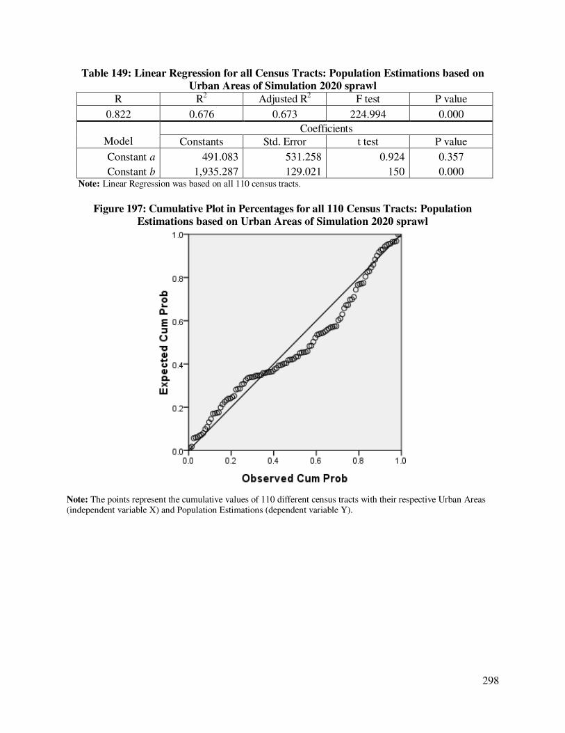
Table 149: Linear Regression for all Census Tracts: Population Estimations based on
Urban Areas of Simulation 2020 sprawl
R R2 Adjusted R
2 F test P value
0.822 0.676 0.673 224.994 0.000
Model
Coefficients
Constants Std. Error t test P value
Constant a 491.083 531.258 0.924 0.357
Constant b
1,935.287 129.021 150 0.000 Note: Linear Regression was based on all 110 census tracts.
Figure 197: Cumulative Plot in Percentages for all 110 Census Tracts: Population
Estimations based on Urban Areas of Simulation 2020 sprawl
Note: The points represent the cumulative values of 110 different census tracts with their respective Urban Areas (independent variable X) and Population Estimations (dependent variable Y).

299
Table 150: Linear Regression for all Census Tracts: Population Estimations based on
Urban Areas of Simulation 2025 smart
R R2 Adjusted R
2 F test P value
0.778 0.605 0.601 165.229 0.000
Model
Coefficients
Constants Std. Error t test P value
Constant a -52.888 697.436 -0.076 0.940
Constant b
3,096.878 240.924 12.854 0.000 Note: Linear Regression was based on all 110 census tracts.
Figure 198: Cumulative Plot in Percentages for all 110 Census Tracts: Population
Estimations based on Urban Areas of Simulation 2025 smart
Note: The points represent the cumulative values of 110 different census tracts with their respective Urban Areas (independent variable X) and Population Estimations (dependent variable Y).
300
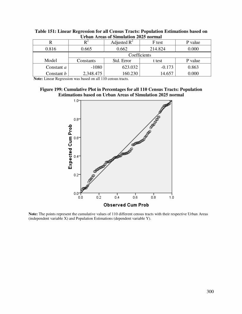
Table 151: Linear Regression for all Census Tracts: Population Estimations based on
Urban Areas of Simulation 2025 normal
R R2 Adjusted R
2 F test P value
0.816 0.665 0.662 214.824 0.000
Model
Coefficients
Constants Std. Error t test P value
Constant a -1080 623.032 -0.173 0.863
Constant b
2,348.475 160.230 14.657 0.000 Note: Linear Regression was based on all 110 census tracts.
Figure 199: Cumulative Plot in Percentages for all 110 Census Tracts: Population
Estimations based on Urban Areas of Simulation 2025 normal
Note: The points represent the cumulative values of 110 different census tracts with their respective Urban Areas (independent variable X) and Population Estimations (dependent variable Y).

301
Table 152: Linear Regression for all Census Tracts: Population Estimations based on
Urban Areas of Simulation 2025 sprawl
R R2 Adjusted R
2 F test P value
0.824 0.680 0.677 229.139 0.000
Model
Coefficients
Constants Std. Error t test P value
Constant a -28.059 600.646 -0.047 0.963
Constant b
2,013.318 133.003 15.137 0.000 Note: Linear Regression was based on all 110 census tracts.
Figure 200: Cumulative Plot in Percentages for all 110 Census Tracts: Population
Estimations based on Urban Areas of Simulation 2025 sprawl
Note: The points represent the cumulative values of 110 different census tracts with their respective Urban Areas (independent variable X) and Population Estimations (dependent variable Y).
302
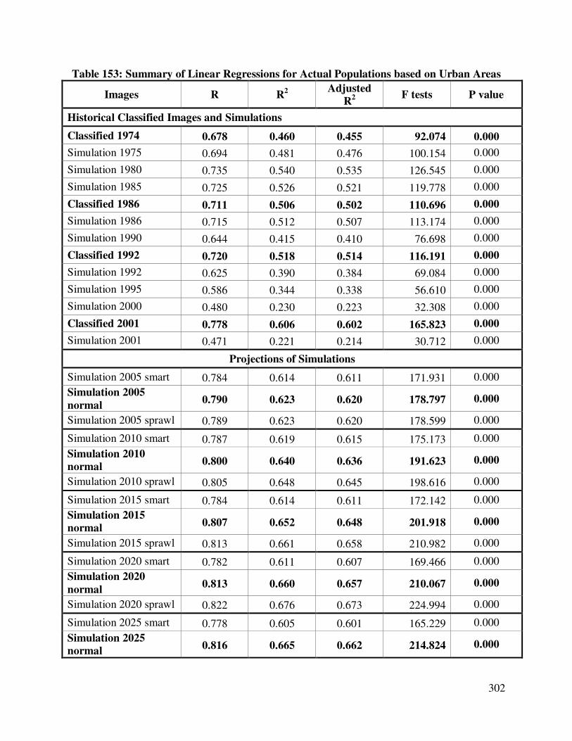
Table 153: Summary of Linear Regressions for Actual Populations based on Urban Areas
Images R R2
Adjusted
R2
F tests P value
Historical Classified Images and Simulations
Classified 1974 0.678 0.460 0.455 92.074 0.000
Simulation 1975 0.694 0.481 0.476 100.154 0.000
Simulation 1980 0.735 0.540 0.535 126.545 0.000
Simulation 1985 0.725 0.526 0.521 119.778 0.000
Classified 1986 0.711 0.506 0.502 110.696 0.000
Simulation 1986 0.715 0.512 0.507 113.174 0.000
Simulation 1990 0.644 0.415 0.410 76.698 0.000
Classified 1992 0.720 0.518 0.514 116.191 0.000
Simulation 1992 0.625 0.390 0.384 69.084 0.000
Simulation 1995 0.586 0.344 0.338 56.610 0.000
Simulation 2000 0.480 0.230 0.223 32.308 0.000
Classified 2001 0.778 0.606 0.602 165.823 0.000
Simulation 2001 0.471 0.221 0.214 30.712 0.000
Projections of Simulations
Simulation 2005 smart 0.784 0.614 0.611 171.931 0.000
Simulation 2005
normal 0.790 0.623 0.620 178.797 0.000
Simulation 2005 sprawl 0.789 0.623 0.620 178.599 0.000
Simulation 2010 smart 0.787 0.619 0.615 175.173 0.000
Simulation 2010
normal 0.800 0.640 0.636 191.623 0.000
Simulation 2010 sprawl 0.805 0.648 0.645 198.616 0.000
Simulation 2015 smart 0.784 0.614 0.611 172.142 0.000
Simulation 2015
normal 0.807 0.652 0.648 201.918 0.000
Simulation 2015 sprawl 0.813 0.661 0.658 210.982 0.000
Simulation 2020 smart 0.782 0.611 0.607 169.466 0.000
Simulation 2020
normal 0.813 0.660 0.657 210.067 0.000
Simulation 2020 sprawl 0.822 0.676 0.673 224.994 0.000
Simulation 2025 smart 0.778 0.605 0.601 165.229 0.000
Simulation 2025
normal 0.816 0.665 0.662 214.824 0.000
303
Simulation 2025 sprawl 0.824 0.680 0.677 229.139 0.000
Notes: Just the land cover of urbanized pixels is used in the Classified Images and Simulations. The independent variable (X) is Constant b and the dependent variable (Y) is Population Estimations.
Classified Image Classified Images and Simulations with normal trend growth are highlighted with black
color and they constitute control parameters.
In Table 153 notice that the higher the F test, also the higher the values of correlations and
coefficient of determination will be. Is important, that the F test results for all linear regressions
present P values < 0.05; therefore, all regression models reject their null hypothesis (H0) and
population values do not result from chance, but instead from urbanized pixels measured in Km2
within each one of the 110 census tracts.
Among all classified images, the image from 2001 shows the highest correlation coefficient
(R=77.8%), and between 60.6% (according to R2) and 60.2% (considering adjusted R
2) of the
variation in the dependent variable Population (Y) can be explained by the independent variable
Urban Areas (X), whereas the remaining percentage (between 39.4% and 39.8%) can be
explained by unknown, extraneous values or inherent variability.
The classified image 1992 also presents a high correlation coefficient (R=72.0%), but the
coefficient of determination (R2=51.8%) and adjusted coefficient of determination (adjusted
R2=51.4%) which explain the variation in the dependent variable Population (Y) by the
independent variable Urban Areas (X) are much lower compared against the classified image
from 2001, whereas the remaining percentage (between 48.2% and 48.6%) can be explained by
unknown, extraneous values or inherent variability.
The classified image 1986 presents very similar statistics than the classified image from 1986
with a slightly smaller correlation coefficient (R=71.1%), and with similar coefficients of
determination (R2=50.6%) and adjusted coefficient of determination (adjusted R
2=50.2%). In this
image from 1986 the remaining percentage (between 49.4% and 49.8%) can be explained by
unknown, extraneous values or inherent variability.
The classified image 1974 presents among the group of all four classified images the smaller
correlation coefficient (R=67.8%) and very poor values for the coefficient of determination
(R2=46.0%) and adjusted coefficient of determination (adjusted R
2=45.5%), and here most of the
percentage (between 54.0% and 54.5%) can be explained by unknown, extraneous values or
inherent variability.
The main reason for these classified images having higher R, R
2 and adjusted R
2 values than
others, is that when their accuracy was assessed against 1,500 random sample points collected
from high resolution digital photographs in Chapter 2, they also presented different Kappa index
of agreement for their urban land covers. In this context, the classified image 1974 had the
lowest Kappa index for urban land cover (87.89% using land cover 1974 as the reference image
and 78.77% using points 1974 as the reference image) whereas the classified image 2001 has the
highest Kappa index for urban areas (93.30% using land cover 2001 as the reference image and
85.79% using points 2001 as the reference image) and identically, the image from 1974 also has
the lowest coefficients of correlation and determination while the image from 2001 shows the
best correlation and regression results. Nevertheless, in the case of the classified images from
304
1986 and 1992, the results not necessarily match this pattern; instead according to the Kappa
indexes, the correlation and regression values from the image of 1986 (91.28% using land cover
1974 as the reference image and 84.36% using points 1974 as the reference image) are higher
than expected in relation to the ones from the image of 1992 (84.37% using land cover 1974 as
the reference image and 79.56% using points 1974 as the reference image).
Among the group of the historical simulated images from 1975 until 2001, Simulation 1980
has the highest correlation coefficient (R=73.5%), coefficient of determination (R2=54.0%) and
adjusted coefficient of determination (adjusted R2=53.5%) between urban areas and population.
The next best values present Simulation 1985 with R=72.5%, R2=52.6% and adjusted R
2=52.1%.
Slightly lower values present Simulation 1986, with R=71.5%, R2=51.2% and adjusted
R2=50.7%.
The rest of simulations present low values for their correlations and very poor statistics
(below the threshold of 50%) for their coefficients of determinations and adjusted coefficient of
determination. In this scenario, Simulation 1975 presents a correlation coefficient of R=69.4%,
while its R2 and adjust R
2 are 48.1% and 47.6% respectively. Simulation 1990 have R=64.44%,
R2=41.5% and adjusted R
2=41.0%. Simulation 1992 presents also similar values to the ones of
Simulation 1990: R=62.5%, R2=39.0% and adjusted R
2=38.4%. Simulation 1995 has R=58.6%,
R2=34.4% and adjusted R
2=33.8%. The historical simulations with the lowest values are the last
ones, from years 2000 and 2001. For example, Simulation 2000 presents the following values:
R=48.05, R2=23.0% and adjusted R2=22.3% whereas simulation 2001 has R=47.1%, R2=22.1%
and adjusted R2=21.4%. In all these cases the remaining percentage (more than 50%) can be
explained by unknown, extraneous values or inherent variability.
The reason these simulations present higher values than others is because of small errors
which accumulate over time through the simulation process from 1974 until 2001. These errors
were already evaluated in Chapter 3 through error matrices and kappa indexes of agreement,
comparing the collected 1,500 sample points from high resolution photographs against the
SLEUTH simulations for years 1986, 1992 and 2001, not being possible to have kappa indexes
for all simulations. In this scenario, the closer in time (number of years) the simulation is from its
beginning (year 1974), in general the higher will be its correlation and coefficient of
determination; in the other hand, the farther away the simulation is from in time from its
beginning in 1974, in general the lower will be its correlation and coefficient of determination.
Consequently, Simulation 1986 have the highest Kappa index for urban land cover (90.17%
using land cover 1974 as the reference image and 82.49% using points 1974 as the reference
image) as well as one of the highest values for R, R2 and adjusted R2 among all historical
simulations. The Simulation 1992 have a middle Kappa index for urban land cover (87.20%
using land cover 1974 as the reference image and 76.94% using points 1974 as the reference
image). And finally, Simulation 2001 has the lowest Kappa index for urban areas (93.30% using
land cover 2001 as the reference image and 85.79% using points 2001 as the reference image),
coinciding these values also with the lowest values for R, R2 and adjusted R2 for this last
historical simulation.
Even if the values of the historical simulations are generally poor, the values of the
simulations into the future made from the last classified image of 2001 into the future (2025) are
305
quite high, with the highest coefficients for smart growth in 2010, whereas normal trend and
urban sprawl simulations have astonishing their highest measures for year 2025.
The smart growth simulation in 2005 presents the following values: R=78.4%, R2=61.4% and
adjusted R2=61.1%. This same trend in the simulation 2010 will barely increase to R=78.7%,
R2=61.9% and adjusted R
2=61.5%, slightly diminishing for 2015 to R=78.4%, R
2=61.4% and
adjusted R2=61.1%. For 2020, the smart growth trend will still diminish to R=78.2%, R
2=61.1%
and adjusted R2=60.7% and these values will be a little bit lower for this trend in simulation
2025: R=77.8%, R2=60.5% and adjusted R
2=60.1%. Therefore, always in the smart growth trend
for all simulations, the unexplained, extraneous values or inherent variability will be below 33%
for correlations (R) and below 40% for R2 and adjusted R
2.
The normal trend simulation in 2005 presents these values: R=79.0%, R2=62.3% and adjusted
R2=62.0%. This same trend in the Simulation 2010 will increase to R=80.0%, R
2=64.0% and
adjusted R2=63.6%. These small increments will remain until 2025, presenting the normal trend
simulation in 2015 these values: R=80.7%, R2=65.2% and adjusted R
2=64.8%; in 2020
R=81.3%, R2=66.0% and adjusted R
2=65.7% and finally as it was mentioned before, the highest
value will be for the normal trend simulation in 2025, when R=81.6%, R2=66.5% and adjusted
R2=66.2%. Consequently, generally for normal trend simulations, the unexplained, extraneous
values or inherent variability will be below 32% for correlations coefficients (R) and below 38%
for coefficients of determinations (R2) and adjusted R
2.
Finally, in the case of the urban sprawl simulations, they present the higher correlations and
coefficients of determinations among all simulations. In 2005, the urban sprawl simulation
presented R=78.9, R2=62.3% and adjusted R
2=62.0%. These values will progressively increase
in this trend until year 2025. Following this trend, for 2010, the urban sprawl simulation will
have R=80.5, R2=64.8% and adjusted R
2=64.5%. This same trend in the simulation of 2015 will
present the following values: R=81.3, R2=66.1% and adjusted R
2=65.8%. For 2020, these
measures will slightly increase to R=82.2, R2=67.6% and adjusted R
2=67.3% and finally for the
urban sprawl simulation in 2025 will present its highest coefficients: R=82.4, R2=68.0% and
adjusted R2=67.7%. In this urban sprawl scenario, always the unexplained, extraneous values or
inherent variability will be below 31% for correlations (R) and below 37% for R2 and adjusted
R2.
It is more difficult to explain based on solid proofs the behavior of simulations into the future
because of the lack of physical evidence (imagery). Nevertheless, because of the linear
regression model, it is possible that the coefficients of correlation and regression for the
simulation based on smart growth trend will be higher near the beginning of the simulation
process (year 2001) because this trend tends to increase just slightly the number of urbanized
pixels; consequently, increasing population densities and the differences in the cloud of points
(represented by census tracts) in relation with the regression line. These differences are more
difficult to evaluate when the graphics are made of cumulative frequencies instead of raw values,
as is the case in this dissertation; nevertheless, this differences are showed in the values of R, R2
and adjusted R2.
306
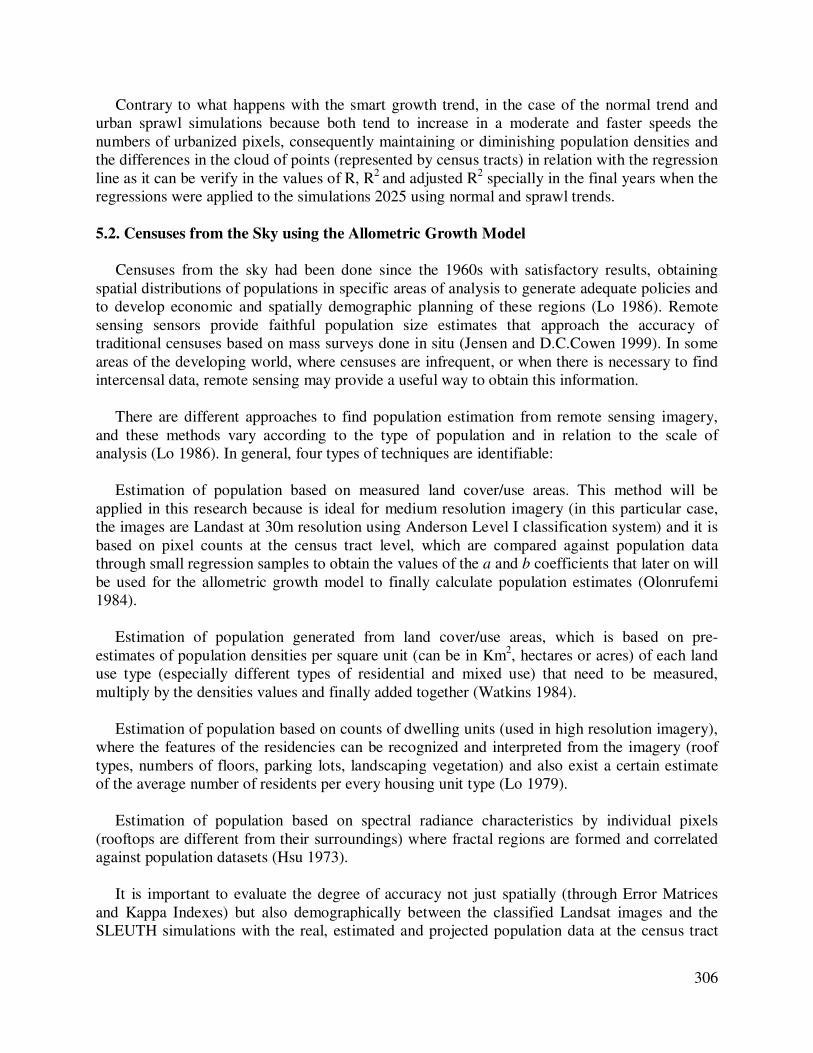
Contrary to what happens with the smart growth trend, in the case of the normal trend and
urban sprawl simulations because both tend to increase in a moderate and faster speeds the
numbers of urbanized pixels, consequently maintaining or diminishing population densities and
the differences in the cloud of points (represented by census tracts) in relation with the regression
line as it can be verify in the values of R, R2
and adjusted R2 specially in the final years when the
regressions were applied to the simulations 2025 using normal and sprawl trends.
5.2. Censuses from the Sky using the Allometric Growth Model
Censuses from the sky had been done since the 1960s with satisfactory results, obtaining
spatial distributions of populations in specific areas of analysis to generate adequate policies and
to develop economic and spatially demographic planning of these regions (Lo 1986). Remote
sensing sensors provide faithful population size estimates that approach the accuracy of
traditional censuses based on mass surveys done in situ (Jensen and D.C.Cowen 1999). In some
areas of the developing world, where censuses are infrequent, or when there is necessary to find
intercensal data, remote sensing may provide a useful way to obtain this information.
There are different approaches to find population estimation from remote sensing imagery,
and these methods vary according to the type of population and in relation to the scale of
analysis (Lo 1986). In general, four types of techniques are identifiable:
Estimation of population based on measured land cover/use areas. This method will be
applied in this research because is ideal for medium resolution imagery (in this particular case,
the images are Landast at 30m resolution using Anderson Level I classification system) and it is
based on pixel counts at the census tract level, which are compared against population data
through small regression samples to obtain the values of the a and b coefficients that later on will
be used for the allometric growth model to finally calculate population estimates (Olonrufemi
1984).
Estimation of population generated from land cover/use areas, which is based on pre-
estimates of population densities per square unit (can be in Km2, hectares or acres) of each land
use type (especially different types of residential and mixed use) that need to be measured,
multiply by the densities values and finally added together (Watkins 1984).
Estimation of population based on counts of dwelling units (used in high resolution imagery),
where the features of the residencies can be recognized and interpreted from the imagery (roof
types, numbers of floors, parking lots, landscaping vegetation) and also exist a certain estimate
of the average number of residents per every housing unit type (Lo 1979).
Estimation of population based on spectral radiance characteristics by individual pixels
(rooftops are different from their surroundings) where fractal regions are formed and correlated
against population datasets (Hsu 1973).
It is important to evaluate the degree of accuracy not just spatially (through Error Matrices
and Kappa Indexes) but also demographically between the classified Landsat images and the
SLEUTH simulations with the real, estimated and projected population data at the census tract
307
level. Therefore, in order to generate these comparisons is necessary to use just the urban pixels
(the only ones that contain population) within the census tracts from the maps already generated
in the classified images and SLEUTH simulations. This statistical technique is called Censuses
from the Sky, and it consists of two steps: First, in applying a linear regression to a small sample
compose of a few census tracts (just 10 were selected in this particular case) containing the
number of urbanized pixels (spatial independent variable X) and the demographic data (statistical
dependent variable Y) to obtain the unknowns a and b coefficients. The second step consists on
using these two coefficients into the allometric growth model to derive the population
estimations. Finally, the actual or real population values are compared against the estimated
population values that resulted from the application of the allometric growth model (censuses
from the sky) using their differences in absolute and percentage values as well as the Root Mean
Square Error (RMSE).
This research compares the estimated populations obtained in the censuses from the sky
through the allometric growth model (logarithmic linear regression) against the actual
populations obtained through the dasymetric density method in Chapter 4; but, if densities from
these two methods will be compared as well, it will be possible to appreciate that always the
linear regressions used in the censuses from the sky tend to smooth the density gaps among the
different census tracts, because depending on the urban configuration of the city in a certain
moment of time (different zones, different residential densities, different heights of buildings
within a census tract and among them) is possible that in reality the best regression pattern for
the cloud of points is not necessarily linear, but instead a power, cubic or quadratic regression.
5.2.1. Linear Regression Model for just 10 Census Tracts
The main idea behind this process also known as model calibration is to apply a linear
regression to a small sample of censuses tracts (just 10 of them were selected: numbers 10, 20,
30, 40, 50, 60, 70, 80, 90 and 100) with their correspondence number of urbanized pixels as well
as their demographic values, in order to obtain the unknowns a (y-intercept of the regression line
or the value of Y when X = 0) and b coefficients (the slope of the regression line).
As it was mentioned before, the input data for this linear regression model consist of two
kinds of data: first, the count of the number of urbanized pixels in every census tract obtained
from urban land cover through satellite image classification or SLEUTH simulation (spatial
independent variable X); and second, the statistics about population for every census tract
obtained from censuses (Geolytics) and estimated or projected from known values (statistical
dependent variable Y).
In this particular case, the formula used for the linear regression equation is identical to the
one used before at the beginning of this chapter for the regression of the 110 census tracts, where
the independent variable X consists on the Area of Urban Pixels in Km2 whereas its dependent
variable Y constitutes the Actual Population.
These regression samples, many times the P values are higher than the 5% threshold, (P <
0.05); nevertheless, it does not really matters because it is well known that when the regression
308
coefficient is applied for all 110 census tracts, the P value is zero (0), so the population data
(independent variable Y) does not exist by chance and the null hypothesis (H0) is rejected.
In these linear regression samples, what matters the most is to obtain the values of the a and b
coefficients that later on will be used for the calculation of the allometric growth model.
Therefore, the results of the correlation coefficients (R), coefficient of determination (R2),
adjusted coefficient of determination (adjusted R2), t tests, F test and P values will not be
analyzed in a summary table at the end of the regression models, instead the next point will be
the calculation of the allometric growth model to generate the census form the sky and obtain the
estimated populations. Finally these results will be compared against the actual populations in a
summary table to assess the accuracy of the classified images and SLEUTH simulations in the
prediction of demographic data.

309
Table 154: Linear Regression for 10 Census Tracts: Population Estimations based on
Urban Areas of Classified Image 1974
R R2 Adjusted R
2 F test P value
0.854 0.729 0.696 21.564 0.002
Model
Coefficients
Constants Std. Error t test P value
Constant a 3.421 0.043 78.925 0.000
Constant b 1.366 0.294 4.644 0.002
Notes: Linear regression was based on just 10 selected census tracts. Therefore, R, R Square, Adjusted R Square and the Std. Error of the Estimate are just partial results. a and b coefficients are very important values that will be used after in the allometric growth model.
Figure 201: Cumulative Plot in Percentages for 10 Census Tracts: Population Estimations
based on Urban Areas of Classified Image 1974
Note: The points represent the cumulative values of 10 different census tracts with their respective Urban Areas
(independent variable X) and Population Estimations (dependent variable Y).
310
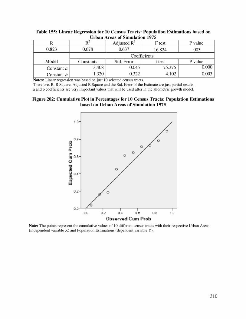
Table 155: Linear Regression for 10 Census Tracts: Population Estimations based on
Urban Areas of Simulation 1975
R R2 Adjusted R
2 F test P value
0.823 0.678 0.637 16.824 .003
Model
Coefficients
Constants Std. Error t test P value
Constant a 3.408 0.045 75.375 0.000
Constant b 1.320 0.322 4.102 0.003
Notes: Linear regression was based on just 10 selected census tracts. Therefore, R, R Square, Adjusted R Square and the Std. Error of the Estimate are just partial results. a and b coefficients are very important values that will be used after in the allometric growth model.
Figure 202: Cumulative Plot in Percentages for 10 Census Tracts: Population Estimations
based on Urban Areas of Simulation 1975
Note: The points represent the cumulative values of 10 different census tracts with their respective Urban Areas
(independent variable X) and Population Estimations (dependent variable Y).

311
Table 156: Linear Regression for 10 Census Tracts: Population Estimations based on
Urban Areas of Simulation 1980
R R2 Adjusted R
2 F test P value
0.644 0.414 0.341 5.655 .045
Model
Coefficients
Constants Std. Error t test P value
Constant a 3.406 0.058 59.183 0.000
Constant b 1.007 0.423 2.378 0.045
Notes: Linear regression was based on just 10 selected census tracts. Therefore, R, R Square, Adjusted R Square and the Std. Error of the Estimate are just partial results. a and b coefficients are very important values that will be used after in the allometric growth model.
Figure 203: Cumulative Plot in Percentages for 10 Census Tracts: Population Estimations
based on Urban Areas of Simulation 1980
Note: The points represent the cumulative values of 10 different census tracts with their respective Urban Areas
(independent variable X) and Population Estimations (dependent variable Y).

312
Table 157: Linear Regression for 10 Census Tracts: Population Estimations based on
Urban Areas of Simulation 1985
R R2 Adjusted R
2 F test P value
0.592 0.350 0.269 4.313 0.071
Model
Coefficients
Constants Std. Error t test P value
Constant a 3.450 0.063 55.002 0.000
Constant b .867 0.418 2.077 0.071
Notes: Linear regression was based on just 10 selected census tracts. Therefore, R, R Square, Adjusted R Square and the Std. Error of the Estimate are just partial results. a and b coefficients are very important values that will be used after in the allometric growth model.
Figure 204: Cumulative Plot in Percentages for 10 Census Tracts: Population Estimations
based on Urban Areas of Simulation 1985
Note: The points represent the cumulative values of 10 different census tracts with their respective Urban Areas
(independent variable X) and Population Estimations (dependent variable Y).

313
Table 158: Linear Regression for 10 Census Tracts: Population Estimations based on
Urban Areas of Classified Image 1986
R R2 Adjusted R
2 F test P value
0.509 0.259 0.167 2.803 0.133
Model
Coefficients
Constants Std. Error t test P value
Constant a 3.474 0.066 52.747 0.000
Constant b 0.491 0.293 1.674 0.133
Notes: Linear regression was based on just 10 selected census tracts. Therefore, R, R Square, Adjusted R Square and the Std. Error of the Estimate are just partial results. a and b coefficients are very important values that will be used after in the allometric growth model.
Figure 205: Cumulative Plot in Percentages for 10 Census Tracts: Population Estimations
based on Urban Areas of Classified Image 1986
Note: The points represent the cumulative values of 10 different census tracts with their respective Urban Areas
(independent variable X) and Population Estimations (dependent variable Y).
314
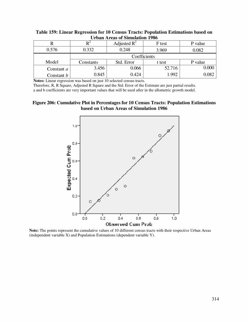
Table 159: Linear Regression for 10 Census Tracts: Population Estimations based on
Urban Areas of Simulation 1986
R R2 Adjusted R
2 F test P value
0.576 0.332 0.248 3.969 0.082
Model
Coefficients
Constants Std. Error t test P value
Constant a 3.456 0.066 52.716 0.000
Constant b 0.845 0.424 1.992 0.082
Notes: Linear regression was based on just 10 selected census tracts. Therefore, R, R Square, Adjusted R Square and the Std. Error of the Estimate are just partial results. a and b coefficients are very important values that will be used after in the allometric growth model.
Figure 206: Cumulative Plot in Percentages for 10 Census Tracts: Population Estimations
based on Urban Areas of Simulation 1986
Note: The points represent the cumulative values of 10 different census tracts with their respective Urban Areas
(independent variable X) and Population Estimations (dependent variable Y).
315
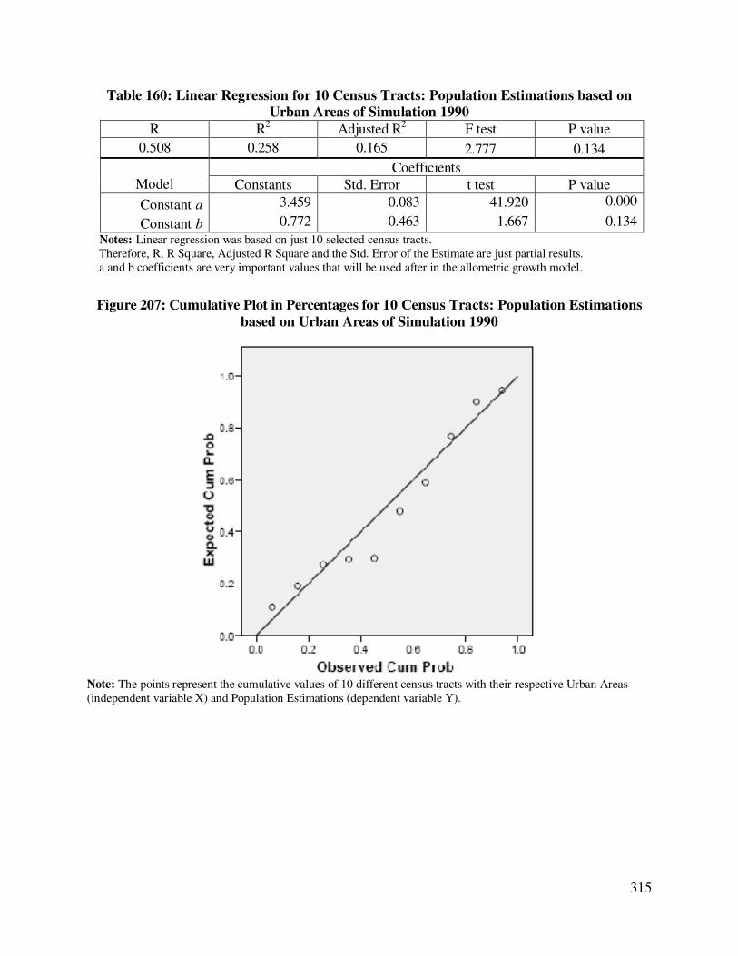
Table 160: Linear Regression for 10 Census Tracts: Population Estimations based on
Urban Areas of Simulation 1990
R R2 Adjusted R
2 F test P value
0.508 0.258 0.165 2.777 0.134
Model
Coefficients
Constants Std. Error t test P value
Constant a 3.459 0.083 41.920 0.000
Constant b 0.772 0.463 1.667 0.134
Notes: Linear regression was based on just 10 selected census tracts. Therefore, R, R Square, Adjusted R Square and the Std. Error of the Estimate are just partial results. a and b coefficients are very important values that will be used after in the allometric growth model.
Figure 207: Cumulative Plot in Percentages for 10 Census Tracts: Population Estimations
based on Urban Areas of Simulation 1990
Note: The points represent the cumulative values of 10 different census tracts with their respective Urban Areas
(independent variable X) and Population Estimations (dependent variable Y).
316
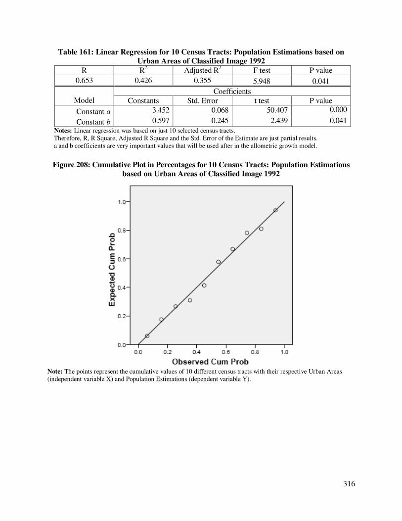
Table 161: Linear Regression for 10 Census Tracts: Population Estimations based on
Urban Areas of Classified Image 1992
R R2 Adjusted R
2 F test P value
0.653 0.426 0.355 5.948 0.041
Model
Coefficients
Constants Std. Error t test P value
Constant a 3.452 0.068 50.407 0.000
Constant b 0.597 0.245 2.439 0.041
Notes: Linear regression was based on just 10 selected census tracts. Therefore, R, R Square, Adjusted R Square and the Std. Error of the Estimate are just partial results. a and b coefficients are very important values that will be used after in the allometric growth model.
Figure 208: Cumulative Plot in Percentages for 10 Census Tracts: Population Estimations
based on Urban Areas of Classified Image 1992
Note: The points represent the cumulative values of 10 different census tracts with their respective Urban Areas
(independent variable X) and Population Estimations (dependent variable Y).

317
Table 162: Linear Regression for 10 Census Tracts: Population Estimations based on
Urban Areas of Simulation 1992
R R2 Adjusted R
2 F test P value
0.510 0.260 0.167 2.807 0.132
Model
Coefficients
Constants Std. Error t test P value
Constant a 3.451 0.090 38.365 0.000
Constant b 0.778 0.464 1.675 0.132
Notes: Linear regression was based on just 10 selected census tracts. Therefore, R, R Square, Adjusted R Square and the Std. Error of the Estimate are just partial results. a and b coefficients are very important values that will be used after in the allometric growth model.
Figure 209: Cumulative Plot in Percentages for 10 Census Tracts: Population Estimations
based on Urban Areas of Simulation 1992
Note: The points represent the cumulative values of 10 different census tracts with their respective Urban Areas
(independent variable X) and Population Estimations (dependent variable Y).
318
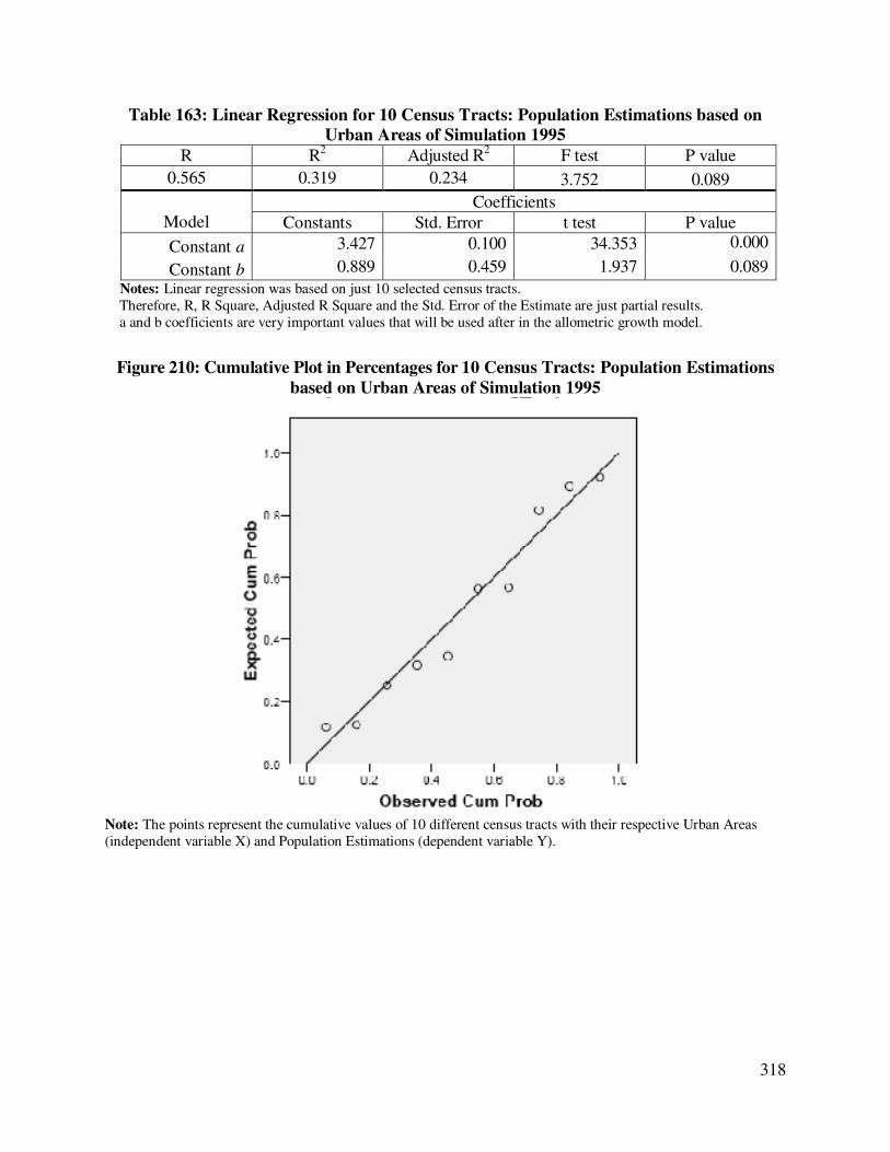
Table 163: Linear Regression for 10 Census Tracts: Population Estimations based on
Urban Areas of Simulation 1995
R R2 Adjusted R
2 F test P value
0.565 0.319 0.234 3.752 0.089
Model
Coefficients
Constants Std. Error t test P value
Constant a 3.427 0.100 34.353 0.000
Constant b 0.889 0.459 1.937 0.089
Notes: Linear regression was based on just 10 selected census tracts. Therefore, R, R Square, Adjusted R Square and the Std. Error of the Estimate are just partial results. a and b coefficients are very important values that will be used after in the allometric growth model.
Figure 210: Cumulative Plot in Percentages for 10 Census Tracts: Population Estimations
based on Urban Areas of Simulation 1995
Note: The points represent the cumulative values of 10 different census tracts with their respective Urban Areas
(independent variable X) and Population Estimations (dependent variable Y).

319
Table 164: Linear Regression for 10 Census Tracts: Population Estimations based on
Urban Areas of Simulation 2000
R R2 Adjusted R
2 F test P value
0.681 0.463 0.396 6.910 0.030
Model
Coefficients
Constants Std. Error t test P value
Constant a 3.332 0.120 27.855 0.000
Constant b 1.219 0.464 2.629 0.030
Notes: Linear regression was based on just 10 selected census tracts. Therefore, R, R Square, Adjusted R Square and the Std. Error of the Estimate are just partial results. a and b coefficients are very important values that will be used after in the allometric growth model.
Figure 211: Cumulative Plot in Percentages for 10 Census Tracts: Population Estimations
based on Urban Areas of Simulation 2000
Note: The points represent the cumulative values of 10 different census tracts with their respective Urban Areas
(independent variable X) and Population Estimations (dependent variable Y).
320
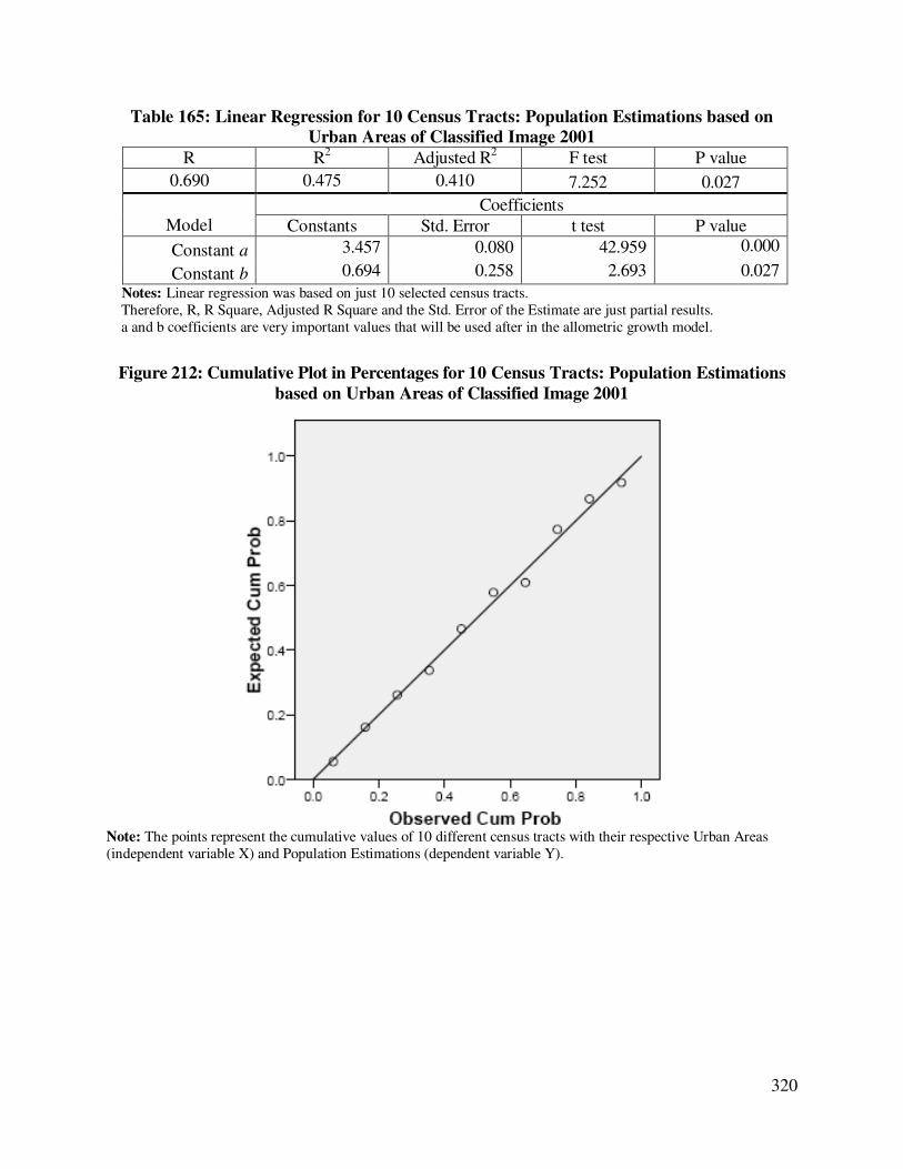
Table 165: Linear Regression for 10 Census Tracts: Population Estimations based on
Urban Areas of Classified Image 2001
R R2 Adjusted R
2 F test P value
0.690 0.475 0.410 7.252 0.027
Model
Coefficients
Constants Std. Error t test P value
Constant a 3.457 0.080 42.959 0.000
Constant b 0.694 0.258 2.693 0.027
Notes: Linear regression was based on just 10 selected census tracts. Therefore, R, R Square, Adjusted R Square and the Std. Error of the Estimate are just partial results. a and b coefficients are very important values that will be used after in the allometric growth model.
Figure 212: Cumulative Plot in Percentages for 10 Census Tracts: Population Estimations
based on Urban Areas of Classified Image 2001
Note: The points represent the cumulative values of 10 different census tracts with their respective Urban Areas
(independent variable X) and Population Estimations (dependent variable Y).

321
Table 166: Linear Regression for 10 Census Tracts: Population Estimations based on
Urban Areas of Simulation 2001
R R2 Adjusted R
2 F test P value
0.692 0.479 0.414 7.348 0.027
Model
Coefficients
Constants Std. Error t test P value
Constant a 3.324 0.121 27.474 0.000
Constant b 1.239 0.457 2.711 0.027
Notes: Linear regression was based on just 10 selected census tracts. Therefore, R, R Square, Adjusted R Square and the Std. Error of the Estimate are just partial results. a and b coefficients are very important values that will be used after in the allometric growth model.
Figure 213: Cumulative Plot in Percentages for 10 Census Tracts: Population Estimations
based on Urban Areas of Simulation 2001
Note: The points represent the cumulative values of 10 different census tracts with their respective Urban Areas
(independent variable X) and Population Estimations (dependent variable Y).

322
Table 167: Linear Regression for 10 Census Tracts: Population Estimations based on
Urban Areas of Simulation 2005 smart
R R2 Adjusted R
2 F test P value
0.698 0.487 0.423 7.599 0.025
Model
Coefficients
Constants Std. Error t test P value
Constant a 3.466 0.085 40.801 0.000
Constant b 0.733 0.266 2.757 0.025
Notes: Linear regression was based on just 10 selected census tracts. Therefore, R, R Square, Adjusted R Square and the Std. Error of the Estimate are just partial results. a and b coefficients are very important values that will be used after in the allometric growth model.
Figure 214: Cumulative Plot in Percentages for 10 Census Tracts: Population Estimations
based on Urban Areas of Simulation 2005 smart
Note: The points represent the cumulative values of 10 different census tracts with their respective Urban Areas
(independent variable X) and Population Estimations (dependent variable Y).

323
Table 168: Linear Regression for 10 Census Tracts: Population Estimations based on
Urban Areas of Simulation 2005 normal
R R2 Adjusted R
2 F test P value
0.702 0.493 0.430 7.779 0.024
Model
Coefficients
Constants Std. Error t test P value
Constant a 3.451 0.088 39.002 0.000
Constant b 0.748 0.268 2.789 0.024
Notes: Linear regression was based on just 10 selected census tracts. Therefore, R, R Square, Adjusted R Square and the Std. Error of the Estimate are just partial results. a and b coefficients are very important values that will be used after in the allometric growth model.
Figure 215: Cumulative Plot in Percentages for 10 Census Tracts: Population Estimations
based on Urban Areas of Simulation 2005 normal
Note: The points represent the cumulative values of 10 different census tracts with their respective Urban Areas
(independent variable X) and Population Estimations (dependent variable Y).

324
Table 169: Linear Regression for 10 Census Tracts: Population Estimations based on
Urban Areas of Simulation 2005 sprawl
R R2 Adjusted R
2 F test P value
0.711 0.506 0.444 8.194 0.021
Model
Coefficients
Constants Std. Error t test P value
Constant a 3.437 0.090 38.005 0.000
Constant b 0.752 0.263 2.862 0.021
Notes: Linear regression was based on just 10 selected census tracts. Therefore, R, R Square, Adjusted R Square and the Std. Error of the Estimate are just partial results. a and b coefficients are very important values that will be used after in the allometric growth model.
Figure 216: Cumulative Plot in Percentages for 10 Census Tracts: Population Estimations
based on Urban Areas of Simulation 2005 sprawl
Note: The points represent the cumulative values of 10 different census tracts with their respective Urban Areas
(independent variable X) and Population Estimations (dependent variable Y).

325
Table 170: Linear Regression for 10 Census Tracts: Population Estimations based on
Urban Areas of Simulation 2010 smart
R R2 Adjusted R
2 F test P value
0.683 0.467 0.400 7.004 0.029
Model
Coefficients
Constants Std. Error t test P value
Constant a 3.491 0.093 37.537 0.000
Constant b 0.764 0.289 2.646 0.029
Notes: Linear regression was based on just 10 selected census tracts. Therefore, R, R Square, Adjusted R Square and the Std. Error of the Estimate are just partial results. a and b coefficients are very important values that will be used after in the allometric growth model.
Figure 217: Cumulative Plot in Percentages for 10 Census Tracts: Population Estimations
based on Urban Areas of Simulation 2010 smart
Note: The points represent the cumulative values of 10 different census tracts with their respective Urban Areas
(independent variable X) and Population Estimations (dependent variable Y).

326
Table 171: Linear Regression for 10 Census Tracts: Population Estimations based on
Urban Areas of Simulation 2010 normal
R R2 Adjusted R
2 F test P value
0.703 0.494 0.431 7.819 0.023
Model
Coefficients
Constants Std. Error t test P value
Constant a 3.443 0.102 33.596 0.000
Constant b 0.806 0.288 2.796 0.023
Notes: Linear regression was based on just 10 selected census tracts. Therefore, R, R Square, Adjusted R Square and the Std. Error of the Estimate are just partial results. a and b coefficients are very important values that will be used after in the allometric growth model.
Figure 218: Cumulative Plot in Percentages for 10 Census Tracts: Population Estimations
based on Urban Areas of Simulation 2010 normal
Note: The points represent the cumulative values of 10 different census tracts with their respective Urban Areas
(independent variable X) and Population Estimations (dependent variable Y).

327
Table 172: Linear Regression for 10 Census Tracts: Population Estimations based on
Urban Areas of Simulation 2010 sprawl
R R2 Adjusted R
2 F test P value
0.728 0.530 0.472 9.038 0.017
Model
Coefficients
Constants Std. Error t test P value
Constant a 3.418 0.104 33.020 0.000
Constant b 0.813 0.270 3.006 0.017
Notes: Linear regression was based on just 10 selected census tracts. Therefore, R, R Square, Adjusted R Square and the Std. Error of the Estimate are just partial results. a and b coefficients are very important values that will be used after in the allometric growth model.
Figure 219: Cumulative Plot in Percentages for 10 Census Tracts: Population Estimations
based on Urban Areas of Simulation 2005 sprawl
Note: The points represent the cumulative values of 10 different census tracts with their respective Urban Areas
(independent variable X) and Population Estimations (dependent variable Y).

328
Table 173: Linear Regression for 10 Census Tracts: Population Estimations based on
Urban Areas of Simulation 2015 smart
R R2 Adjusted R
2 F test P value
0.660 0.436 0.366 6.189 0.038
Model
Coefficients
Constants Std. Error t test P value
Constant a 3.509 0.102 34.260 0.000
Constant b 0.784 0.315 2.488 0.038
Notes: Linear regression was based on just 10 selected census tracts. Therefore, R, R Square, Adjusted R Square and the Std. Error of the Estimate are just partial results. a and b coefficients are very important values that will be used after in the allometric growth model.
Figure 220: Cumulative Plot in Percentages for 10 Census Tracts: Population Estimations
based on Urban Areas of Simulation 2015 smart
Note: The points represent the cumulative values of 10 different census tracts with their respective Urban Areas
(independent variable X) and Population Estimations (dependent variable Y).
329
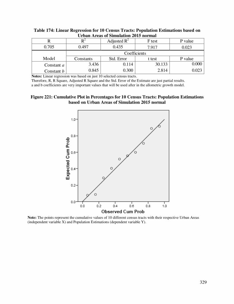
Table 174: Linear Regression for 10 Census Tracts: Population Estimations based on
Urban Areas of Simulation 2015 normal
R R2 Adjusted R
2 F test P value
0.705 0.497 0.435 7.917 0.023
Model
Coefficients
Constants Std. Error t test P value
Constant a 3.436 0.114 30.133 0.000
Constant b 0.845 0.300 2.814 0.023
Notes: Linear regression was based on just 10 selected census tracts. Therefore, R, R Square, Adjusted R Square and the Std. Error of the Estimate are just partial results. a and b coefficients are very important values that will be used after in the allometric growth model.
Figure 221: Cumulative Plot in Percentages for 10 Census Tracts: Population Estimations
based on Urban Areas of Simulation 2015 normal
Note: The points represent the cumulative values of 10 different census tracts with their respective Urban Areas
(independent variable X) and Population Estimations (dependent variable Y).
330
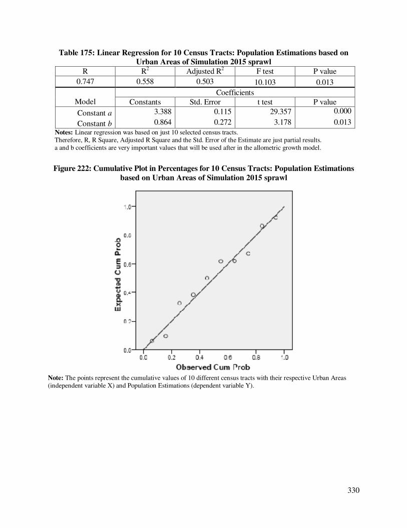
Table 175: Linear Regression for 10 Census Tracts: Population Estimations based on
Urban Areas of Simulation 2015 sprawl
R R2 Adjusted R
2 F test P value
0.747 0.558 0.503 10.103 0.013
Model
Coefficients
Constants Std. Error t test P value
Constant a 3.388 0.115 29.357 0.000
Constant b 0.864 0.272 3.178 0.013
Notes: Linear regression was based on just 10 selected census tracts. Therefore, R, R Square, Adjusted R Square and the Std. Error of the Estimate are just partial results. a and b coefficients are very important values that will be used after in the allometric growth model.
Figure 222: Cumulative Plot in Percentages for 10 Census Tracts: Population Estimations
based on Urban Areas of Simulation 2015 sprawl
Note: The points represent the cumulative values of 10 different census tracts with their respective Urban Areas
(independent variable X) and Population Estimations (dependent variable Y).

331
Table 176: Linear Regression for 10 Census Tracts: Population Estimations based on
Urban Areas of Simulation 2020 smart
R R2 Adjusted R
2 F test P value
0.645 0.415 0.342 5.685 0.044
Model
Coefficients
Constants Std. Error t test P value
Constant a 3.522 0.111 31.701 0.000
Constant b 0.807 0.338 2.384 0.044
Notes: Linear regression was based on just 10 selected census tracts. Therefore, R, R Square, Adjusted R Square and the Std. Error of the Estimate are just partial results. a and b coefficients are very important values that will be used after in the allometric growth model.
Figure 223: Cumulative Plot in Percentages for 10 Census Tracts: Population Estimations
based on Urban Areas of Simulation 2020 smart
Note: The points represent the cumulative values of 10 different census tracts with their respective Urban Areas
(independent variable X) and Population Estimations (dependent variable Y).

332
Table 177: Linear Regression for 10 Census Tracts: Population Estimations based on
Urban Areas of Simulation 2020 normal
R R2 Adjusted R
2 F test P value
0.729 0.532 0.473 9.077 0.017
Model
Coefficients
Constants Std. Error t test P value
Constant a 3.410 0.123 27.813 0.000
Constant b 0.909 0.302 3.013 0.017
Notes: Linear regression was based on just 10 selected census tracts. Therefore, R, R Square, Adjusted R Square and the Std. Error of the Estimate are just partial results. a and b coefficients are very important values that will be used after in the allometric growth model.
Figure 224: Cumulative Plot in Percentages for 10 Census Tracts: Population Estimations
based on Urban Areas of Simulation 2020 normal
Note: The points represent the cumulative values of 10 different census tracts with their respective Urban Areas
(independent variable X) and Population Estimations (dependent variable Y).
333
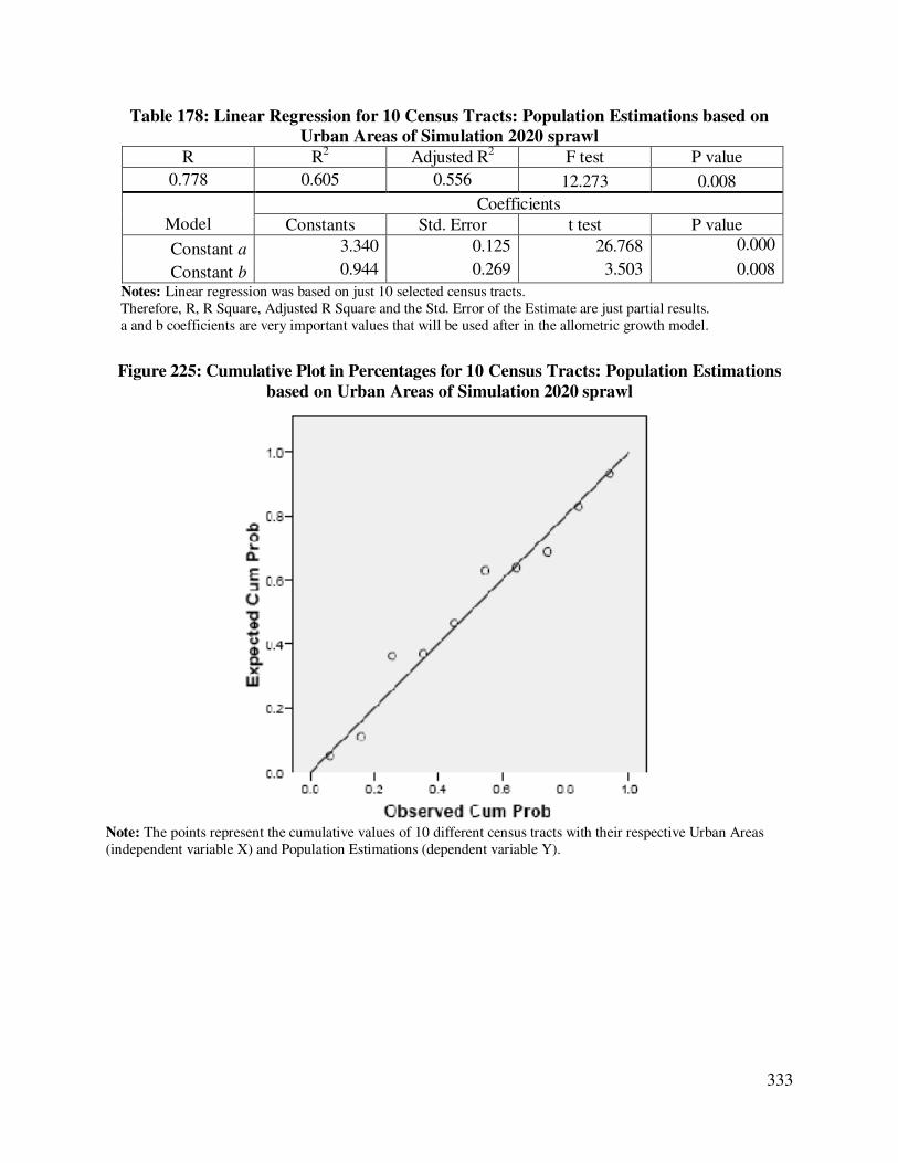
Table 178: Linear Regression for 10 Census Tracts: Population Estimations based on
Urban Areas of Simulation 2020 sprawl
R R2 Adjusted R
2 F test P value
0.778 0.605 0.556 12.273 0.008
Model
Coefficients
Constants Std. Error t test P value
Constant a 3.340 0.125 26.768 0.000
Constant b 0.944 0.269 3.503 0.008
Notes: Linear regression was based on just 10 selected census tracts. Therefore, R, R Square, Adjusted R Square and the Std. Error of the Estimate are just partial results. a and b coefficients are very important values that will be used after in the allometric growth model.
Figure 225: Cumulative Plot in Percentages for 10 Census Tracts: Population Estimations
based on Urban Areas of Simulation 2020 sprawl
Note: The points represent the cumulative values of 10 different census tracts with their respective Urban Areas
(independent variable X) and Population Estimations (dependent variable Y).

334
Table 179: Linear Regression for 10 Census Tracts: Population Estimations based on
Urban Areas of Simulation 2025 smart
R R2 Adjusted R
2 F test P value
0.625 0.390 0.314 5.122 0.053
Model
Coefficients
Constants Std. Error t test P value
Constant a 3.528 0.122 29.016 0.000
Constant b 0.831 0.367 2.263 0.053
Notes: Linear regression was based on just 10 selected census tracts. Therefore, R, R Square, Adjusted R Square and the Std. Error of the Estimate are just partial results. a and b coefficients are very important values that will be used after in the allometric growth model.
Figure 226: Cumulative Plot in Percentages for 10 Census Tracts: Population Estimations
based on Urban Areas of Simulation 2025 normal
Note: The points represent the cumulative values of 10 different census tracts with their respective Urban Areas
(independent variable X) and Population Estimations (dependent variable Y).
335
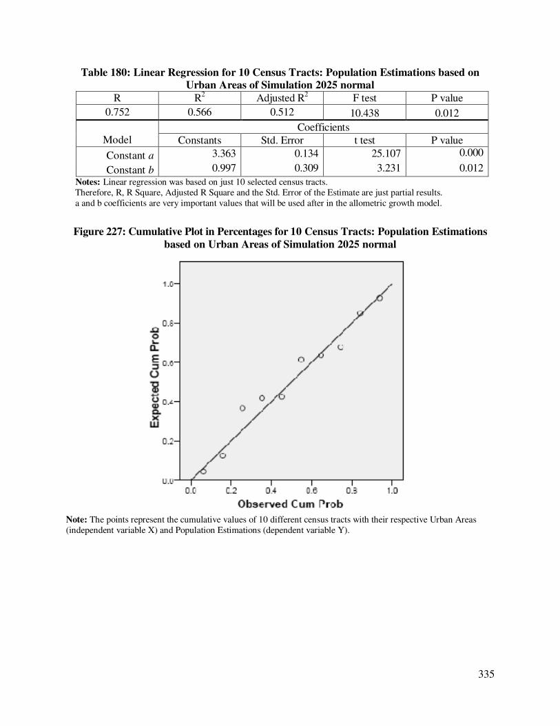
Table 180: Linear Regression for 10 Census Tracts: Population Estimations based on
Urban Areas of Simulation 2025 normal
R R2 Adjusted R
2 F test P value
0.752 0.566 0.512 10.438 0.012
Model
Coefficients
Constants Std. Error t test P value
Constant a 3.363 0.134 25.107 0.000
Constant b 0.997 0.309 3.231 0.012
Notes: Linear regression was based on just 10 selected census tracts. Therefore, R, R Square, Adjusted R Square and the Std. Error of the Estimate are just partial results. a and b coefficients are very important values that will be used after in the allometric growth model.
Figure 227: Cumulative Plot in Percentages for 10 Census Tracts: Population Estimations
based on Urban Areas of Simulation 2025 normal
Note: The points represent the cumulative values of 10 different census tracts with their respective Urban Areas
(independent variable X) and Population Estimations (dependent variable Y).
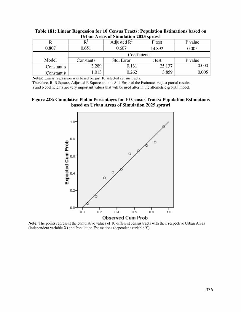
336
Table 181: Linear Regression for 10 Census Tracts: Population Estimations based on
Urban Areas of Simulation 2025 sprawl
R R2 Adjusted R
2 F test P value
0.807 0.651 0.607 14.892 0.005
Model
Coefficients
Constants Std. Error t test P value
Constant a 3.289 0.131 25.137 0.000
Constant b 1.013 0.262 3.859 0.005
Notes: Linear regression was based on just 10 selected census tracts. Therefore, R, R Square, Adjusted R Square and the Std. Error of the Estimate are just partial results. a and b coefficients are very important values that will be used after in the allometric growth model.
Figure 228: Cumulative Plot in Percentages for 10 Census Tracts: Population Estimations
based on Urban Areas of Simulation 2025 sprawl
Note: The points represent the cumulative values of 10 different census tracts with their respective Urban Areas
(independent variable X) and Population Estimations (dependent variable Y).
337
5.2.2. Allometric Growth Model for all 110 Census Tracts
The concept of allometric growth model originally comes from biology and the main idea
behind is that the growth of living organisms (in this case is replaced by cities) is conceived as
the relationship between just two attributes of that organism: in this case it will be its urbanized
areas (independent variable X) and its population (dependent variable Y).
Once constants a and b had been previously determined through a linear regression applied to
just 10 censuses tracts and the a and b coefficients were obtained, right now it is possible to
apply the allometric growth model to estimate populations in all 110 census tracts per image
using Microsoft EXCEL software.
The equation for the allometric growth model is the same as the one from a linear regression
but instead of the absolute X and Y values, this model uses their logarithms. Therefore, it is
necessary to transform first the values corresponding to the area of urban pixels (independent
variable X) into their logarithmic values, and because of this transformation, the estimated
population (dependent variable Y) also will result in logarithmic form. After these
transformations are done, it is possible to apply the allometric growth model to all 110 census
tracts to obtain the estimated population values, which at last need to be converted into their
Antilogarithmic (absolute) values, in a process known as Censuses from the Sky, because the
demographic data was derived from the number of urban pixels in every image.
log Y = a + b * log X has been replaced by: log Pest = a + b * log A
Where:
log Pest is the logarithm of the number of the estimated population (dependent variable Y) that
results from the allometic growth formula. After, log Pest can be easily transformed into Pest (the
estimate number of population) through the use of an Antilogarithmic function. Finally the
values of Pest for every census tract can be added together to obtain the total population of the
whole counties.
a is a regression coefficient obtained initially in the model calibration process for just 10
census tracts and it represents the y-intercept: the value of Y when X = 0.
_ _ _ _
a = Y – b * X has been replaced by: a = Pest – b * A
b is another regression coefficient obtained initially in the model calibration process for just
10 census tracts and it represents the slope of the regression line.
( )( )
( )∑
∑∑∑
−
−=
n
XX
n
YXXY
b2
2
has been replaced by:
( )( )
( )∑ ∑
∑∑∑
−
−=
n
AA
n
PestAPestA
b2
2
*
338
log A is the logarithm of the number of urbanized pixels (independent variable: X). A or Area
is the result of counting just the urbanized pixels (through the use of a binary mask) in every
census tract from the land cover data derived from satellite image classification or from the
SLEUTH simulation.
5.2.3. Accuracy Evaluation of the Censuses form the Sky
Result of the Allometric Growth Model (Censuses from the Sky) is the population estimated
value (Pest) in every census tract, which needs to be added together at the county level and
compared against the real or actual populations values (Pact) that already were acquired from past
censuses (Geolytics) or statistical estimations and projections.
There are basically three types of accuracy evaluations between the estimated and the actual
population values: the differences in absolute numbers between actual and estimated populations,
the differences in percentages between both populations and the Root Mean Square Error
(RMSE) between actual and estimated populations (Sirkin 2006).
The differences in absolute numbers and percentages between actual and estimated
populations were calculated after adding each one of the 110 census tracts values for every one
of the three counties: Escambia, Santa Rosa and Okaloosa. Instead, the RMSE was calculated
first in every one of the 100 census tracts that were unused prior for the model calibration to
obtain the a and b coefficients, and finally these census tracts values were added in each county.
For the RMSE, the individual differences or errors that correspond to the addition of the
vertical distances of each of the points from the regression line are squared and finally divided by
the total number of census tracts (Rogerson 2006), as shown in the following formula:
( )N
PPRMSE
actest∑ −=
2
Where:
RMSE = Root Mean Square Error
Pest = estimated population (derived from the allometric growth model)
Pact = actual population (derived from censuses, estimations and projections)
N = Number of census tracts (in this case 100)
The accuracy evaluation of censuses from the sky has been used in big cities, but it tends to
underestimate their population because of the existence of high buildings especially in the
Central Business District (CBD). The allometric growth model also underestimates or
overestimates the population in middle size towns. Nevertheless, this method had been used
successfully in smaller cities, giving population estimation results very similar to the real census
counts (Lo 1986). Due to the reasons mentioned before, this model has to be calibrated to
339
compute the population of different cities depending on their size and country. For example,
cities in developing countries, Europe or Japan tend to be more concentrated and more densely
populated than cities in the United States.
Other inaccuracies in this model result from the spatial resolution of the pixels; for example,
in a Landsat TM image, a pixel of 30m x 30m may contain people living in isolated small houses
(e.g. 10m x 10m), and due to their small sizes, after the image has been classified, these small
features contained within single pixels may appear as forests or grass, so they will not be
populated and therefore will constitute most of the errors in rural areas.
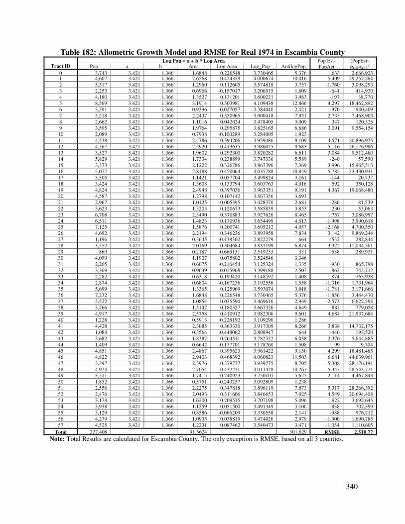
340
Table 182: Allometric Growth Model and RMSE for Real 1974 in Escambia County
Tract ID Log Pop = a + b * Log Area Pop Est-
PopAct
(PopEst-
PopAct)2 Pop a b Area Log Area Log_Pop AntilogPop
0 3,743 3.421 1.366 1.6848 0.226548 3.730465 5,376 1,633 2,666,923 1 4,607 3.421 1.366 2.6568 0.424359 4.000674 10,016 5,409 29,252,264
2 5,517 3.421 1.366 1.2960 0.112605 3.574818 3,757 -1,760 3,098,293
3 2,253 3.421 1.366 0.6966 -0.157017 3.206515 1,609 -644 414,930
4 4,180 3.421 1.366 1.3527 0.131201 3.600221 3,983 -197 38,770
5 8,569 3.421 1.366 3.1914 0.503981 4.109438 12,866 4,297 18,462,892
6 3,391 3.421 1.366 0.9396 -0.027057 3.384040 2,421 -970 940,409
7 5,218 3.421 1.366 2.2437 0.350965 3.900418 7,951 2,733 7,468,903
8 2,662 3.421 1.366 1.1016 0.042024 3.478405 3,009 347 120,325
9 3,595 3.421 1.366 1.9764 0.295875 3.825165 6,686 3,091 9,554,154
10 2,089 3.421 1.366 0.7938 -0.100289 3.284005 1,923
11 4,538 3.421 1.366 2.4786 0.394206 3.959486 9,109 4,571 20,896,975
12 4,567 3.421 1.366 2.5920 0.413635 3.986025 9,683 5,116 26,176,986
13 3,527 3.421 1.366 1.9602 0.292300 3.820282 6,611 3,084 9,512,480
14 5,829 3.421 1.366 1.7334 0.238899 3.747336 5,589 -240 57,590
15 3,373 3.421 1.366 2.1222 0.326786 3.867390 7,369 3,996 15,965,513
16 5,077 3.421 1.366 2.8188 0.450064 4.035788 10,859 5,782 33,430,931
17 3,305 3.421 1.366 1.1421 0.057704 3.499824 3,161 -144 20,737
18 3,424 3.421 1.366 1.3608 0.133794 3.603763 4,016 592 350,128
19 4,824 3.421 1.366 2.4948 0.397036 3.963351 9,191 4,367 19,068,480
20 4,587 3.421 1.366 1.2798 0.107142 3.567356 3,693
21 2,967 3.421 1.366 1.0125 0.005395 3.428370 2,681 -286 81,539
22 3,623 3.421 1.366 1.3203 0.120673 3.585839 3,853 230 53,063
23 6,708 3.421 1.366 2.3490 0.370883 3.927626 8,465 1,757 3,086,997
24 6,511 3.421 1.366 1.4823 0.170936 3.654499 4,513 -1,998 3,990,618
25 7,125 3.421 1.366 1.5876 0.200741 3.695212 4,957 -2,168 4,700,550
26 4,692 3.421 1.366 2.2194 0.346236 3.893958 7,834 3,142 9,869,244
27 1,196 3.421 1.366 0.3645 -0.438302 2.822279 664 -532 282,844
28 3,552 3.421 1.366 2.0169 0.304684 3.837199 6,874 3,322 11,034,561
29 869 3.421 1.366 0.2187 -0.660151 2.519233 331 -538 289,931
30 4,099 3.421 1.366 1.1907 0.075802 3.524546 3,346
31 2,265 3.421 1.366 0.6075 -0.216454 3.125324 1,335 -930 865,798
32 3,369 3.421 1.366 0.9639 -0.015968 3.399188 2,507 -862 742,712
33 2,282 3.421 1.366 0.6318 -0.199420 3.148592 1,408 -874 763,938
34 2,874 3.421 1.366 0.6804 -0.167236 3.192556 1,558 -1,316 1,731,964
35 5,699 3.421 1.366 1.3365 0.125969 3.593074 3,918 -1,781 3,171,666
36 7,232 3.421 1.366 1.6848 0.226548 3.730465 5,376 -1,856 3,444,470
37 5,522 3.421 1.366 1.0854 0.035590 3.469616 2,949 -2,573 6,622,394
38 3,766 3.421 1.366 1.5147 0.180327 3.667326 4,649 883 779,058
39 4,917 3.421 1.366 2.5758 0.410912 3.982306 9,601 4,684 21,937,684
40 1,228 3.421 1.366 0.5913 -0.228192 3.109290 1,286
41 4,428 3.421 1.366 2.3085 0.363330 3.917309 8,266 3,838 14,732,175
42 1,084 3.421 1.366 0.3564 -0.448062 2.808947 644 -440 193,520
43 3,682 3.421 1.366 1.8387 0.264511 3.782322 6,058 2,376 5,644,885
44 1,409 3.421 1.366 0.6642 -0.177701 3.178260 1,508 99 9,704
45 4,851 3.421 1.366 2.4867 0.395623 3.961422 9,150 4,299 18,481,485
46 4,822 3.421 1.366 2.9403 0.468392 4.060823 11,503 6,681 44,639,961
47 3,397 3.421 1.366 2.3976 0.379777 3.939775 8,705 5,308 28,176,191
48 4,924 3.421 1.366 2.7054 0.432231 4.011428 10,267 5,343 28,543,771
49 3,511 3.421 1.366 1.7415 0.240923 3.750101 5,625 2,114 4,467,843
50 1,852 3.421 1.366 0.5751 -0.240257 3.092809 1,238
51 2,556 3.421 1.366 2.2275 0.347818 3.896119 7,873 5,317 28,266,392
52 2,476 3.421 1.366 2.0493 0.311606 3.846653 7,025 4,549 20,694,408
53 3,174 3.421 1.366 1.6200 0.209515 3.707198 5,096 1,922 3,692,645
54 3,938 3.421 1.366 1.1259 0.051500 3.491349 3,100 -838 702,399
55 3,129 3.421 1.366 0.8586 -0.066209 3.330558 2,141 -988 976,712
56 4,279 3.421 1.366 1.0935 0.038819 3.474026 2,979 -1,300 1,690,785
57 4,525 3.421 1.366 1.2231 0.087462 3.540473 3,471 -1,054 1,110,605
Total 227,408 91.5624 301,629 RMSE 2,510.77
Note: Total Results are calculated for Escambia County. The only exception is RMSE, based on all 3 counties.
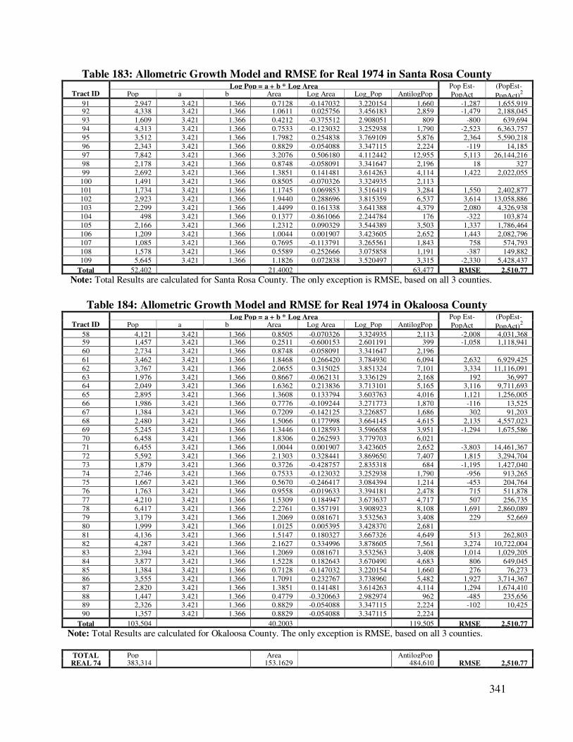
341
Table 183: Allometric Growth Model and RMSE for Real 1974 in Santa Rosa County
Tract ID Log Pop = a + b * Log Area Pop Est-
PopAct
(PopEst-
PopAct)2 Pop a b Area Log Area Log_Pop AntilogPop
91 2,947 3.421 1.366 0.7128 -0.147032 3.220154 1,660 -1,287 1,655,919 92 4,338 3.421 1.366 1.0611 0.025756 3.456183 2,859 -1,479 2,188,045
93 1,609 3.421 1.366 0.4212 -0.375512 2.908051 809 -800 639,694
94 4,313 3.421 1.366 0.7533 -0.123032 3.252938 1,790 -2,523 6,363,757
95 3,512 3.421 1.366 1.7982 0.254838 3.769109 5,876 2,364 5,590,218
96 2,343 3.421 1.366 0.8829 -0.054088 3.347115 2,224 -119 14,185
97 7,842 3.421 1.366 3.2076 0.506180 4.112442 12,955 5,113 26,144,216
98 2,178 3.421 1.366 0.8748 -0.058091 3.341647 2,196 18 327
99 2,692 3.421 1.366 1.3851 0.141481 3.614263 4,114 1,422 2,022,055
100 1,491 3.421 1.366 0.8505 -0.070326 3.324935 2,113
101 1,734 3.421 1.366 1.1745 0.069853 3.516419 3,284 1,550 2,402,877
102 2,923 3.421 1.366 1.9440 0.288696 3.815359 6,537 3,614 13,058,886
103 2,299 3.421 1.366 1.4499 0.161338 3.641388 4,379 2,080 4,326,938
104 498 3.421 1.366 0.1377 -0.861066 2.244784 176 -322 103,874
105 2,166 3.421 1.366 1.2312 0.090329 3.544389 3,503 1,337 1,786,464
106 1,209 3.421 1.366 1.0044 0.001907 3.423605 2,652 1,443 2,082,796
107 1,085 3.421 1.366 0.7695 -0.113791 3.265561 1,843 758 574,793
108 1,578 3.421 1.366 0.5589 -0.252666 3.075858 1,191 -387 149,882
109 5,645 3.421 1.366 1.1826 0.072838 3.520497 3,315 -2,330 5,428,437
Total 52,402 21.4002 63,477 RMSE 2,510.77
Note: Total Results are calculated for Santa Rosa County. The only exception is RMSE, based on all 3 counties.
Table 184: Allometric Growth Model and RMSE for Real 1974 in Okaloosa County
Tract ID Log Pop = a + b * Log Area Pop Est-
PopAct
(PopEst-
PopAct)2 Pop a b Area Log Area Log_Pop AntilogPop
58 4,121 3.421 1.366 0.8505 -0.070326 3.324935 2,113 -2,008 4,031,368 59 1,457 3.421 1.366 0.2511 -0.600153 2.601191 399 -1,058 1,118,941
60 2,734 3.421 1.366 0.8748 -0.058091 3.341647 2,196
61 3,462 3.421 1.366 1.8468 0.266420 3.784930 6,094 2,632 6,929,425
62 3,767 3.421 1.366 2.0655 0.315025 3.851324 7,101 3,334 11,116,091
63 1,976 3.421 1.366 0.8667 -0.062131 3.336129 2,168 192 36,997
64 2,049 3.421 1.366 1.6362 0.213836 3.713101 5,165 3,116 9,711,693
65 2,895 3.421 1.366 1.3608 0.133794 3.603763 4,016 1,121 1,256,005
66 1,986 3.421 1.366 0.7776 -0.109244 3.271773 1,870 -116 13,525
67 1,384 3.421 1.366 0.7209 -0.142125 3.226857 1,686 302 91,203
68 2,480 3.421 1.366 1.5066 0.177998 3.664145 4,615 2,135 4,557,023
69 5,245 3.421 1.366 1.3446 0.128593 3.596658 3,951 -1,294 1,675,586
70 6,458 3.421 1.366 1.8306 0.262593 3.779703 6,021
71 6,455 3.421 1.366 1.0044 0.001907 3.423605 2,652 -3,803 14,461,367
72 5,592 3.421 1.366 2.1303 0.328441 3.869650 7,407 1,815 3,294,704
73 1,879 3.421 1.366 0.3726 -0.428757 2.835318 684 -1,195 1,427,040
74 2,746 3.421 1.366 0.7533 -0.123032 3.252938 1,790 -956 913,265
75 1,667 3.421 1.366 0.5670 -0.246417 3.084394 1,214 -453 204,764
76 1,763 3.421 1.366 0.9558 -0.019633 3.394181 2,478 715 511,878
77 4,210 3.421 1.366 1.5309 0.184947 3.673637 4,717 507 256,735
78 6,417 3.421 1.366 2.2761 0.357191 3.908923 8,108 1,691 2,860,089
79 3,179 3.421 1.366 1.2069 0.081671 3.532563 3,408 229 52,669
80 1,999 3.421 1.366 1.0125 0.005395 3.428370 2,681
81 4,136 3.421 1.366 1.5147 0.180327 3.667326 4,649 513 262,803
82 4,287 3.421 1.366 2.1627 0.334996 3.878605 7,561 3,274 10,722,004
83 2,394 3.421 1.366 1.2069 0.081671 3.532563 3,408 1,014 1,029,205
84 3,877 3.421 1.366 1.5228 0.182643 3.670490 4,683 806 649,045
85 1,384 3.421 1.366 0.7128 -0.147032 3.220154 1,660 276 76,273
86 3,555 3.421 1.366 1.7091 0.232767 3.738960 5,482 1,927 3,714,367
87 2,820 3.421 1.366 1.3851 0.141481 3.614263 4,114 1,294 1,674,410
88 1,447 3.421 1.366 0.4779 -0.320663 2.982974 962 -485 235,656
89 2,326 3.421 1.366 0.8829 -0.054088 3.347115 2,224 -102 10,425
90 1,357 3.421 1.366 0.8829 -0.054088 3.347115 2,224
Total 103,504 40.2003 119,505 RMSE 2,510.77
Note: Total Results are calculated for Okaloosa County. The only exception is RMSE, based on all 3 counties.
TOTAL Pop
Area
AntilogPop REAL 74 383,314 153.1629 484,610 RMSE 2,510.77
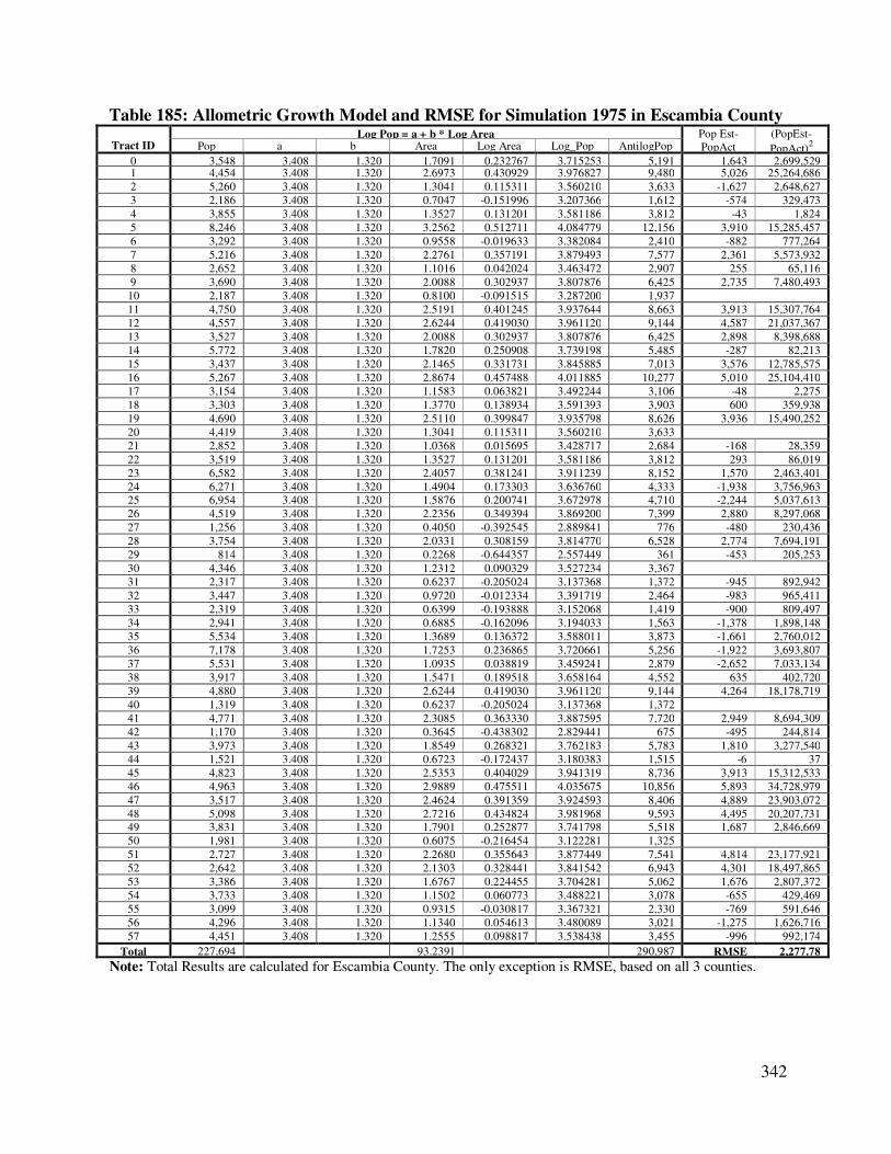
342
Table 185: Allometric Growth Model and RMSE for Simulation 1975 in Escambia County
Tract ID Log Pop = a + b * Log Area Pop Est-
PopAct
(PopEst-
PopAct)2 Pop a b Area Log Area Log_Pop AntilogPop
0 3,548 3.408 1.320 1.7091 0.232767 3.715253 5,191 1,643 2,699,529 1 4,454 3.408 1.320 2.6973 0.430929 3.976827 9,480 5,026 25,264,686
2 5,260 3.408 1.320 1.3041 0.115311 3.560210 3,633 -1,627 2,648,627
3 2,186 3.408 1.320 0.7047 -0.151996 3.207366 1,612 -574 329,473
4 3,855 3.408 1.320 1.3527 0.131201 3.581186 3,812 -43 1,824
5 8,246 3.408 1.320 3.2562 0.512711 4.084779 12,156 3,910 15,285,457
6 3,292 3.408 1.320 0.9558 -0.019633 3.382084 2,410 -882 777,264
7 5,216 3.408 1.320 2.2761 0.357191 3.879493 7,577 2,361 5,573,932
8 2,652 3.408 1.320 1.1016 0.042024 3.463472 2,907 255 65,116
9 3,690 3.408 1.320 2.0088 0.302937 3.807876 6,425 2,735 7,480,493
10 2,187 3.408 1.320 0.8100 -0.091515 3.287200 1,937
11 4,750 3.408 1.320 2.5191 0.401245 3.937644 8,663 3,913 15,307,764
12 4,557 3.408 1.320 2.6244 0.419030 3.961120 9,144 4,587 21,037,367
13 3,527 3.408 1.320 2.0088 0.302937 3.807876 6,425 2,898 8,398,688
14 5,772 3.408 1.320 1.7820 0.250908 3.739198 5,485 -287 82,213
15 3,437 3.408 1.320 2.1465 0.331731 3.845885 7,013 3,576 12,785,575
16 5,267 3.408 1.320 2.8674 0.457488 4.011885 10,277 5,010 25,104,410
17 3,154 3.408 1.320 1.1583 0.063821 3.492244 3,106 -48 2,275
18 3,303 3.408 1.320 1.3770 0.138934 3.591393 3,903 600 359,938
19 4,690 3.408 1.320 2.5110 0.399847 3.935798 8,626 3,936 15,490,252
20 4,419 3.408 1.320 1.3041 0.115311 3.560210 3,633
21 2,852 3.408 1.320 1.0368 0.015695 3.428717 2,684 -168 28,359
22 3,519 3.408 1.320 1.3527 0.131201 3.581186 3,812 293 86,019
23 6,582 3.408 1.320 2.4057 0.381241 3.911239 8,152 1,570 2,463,401
24 6,271 3.408 1.320 1.4904 0.173303 3.636760 4,333 -1,938 3,756,963
25 6,954 3.408 1.320 1.5876 0.200741 3.672978 4,710 -2,244 5,037,613
26 4,519 3.408 1.320 2.2356 0.349394 3.869200 7,399 2,880 8,297,068
27 1,256 3.408 1.320 0.4050 -0.392545 2.889841 776 -480 230,436
28 3,754 3.408 1.320 2.0331 0.308159 3.814770 6,528 2,774 7,694,191
29 814 3.408 1.320 0.2268 -0.644357 2.557449 361 -453 205,253
30 4,346 3.408 1.320 1.2312 0.090329 3.527234 3,367
31 2,317 3.408 1.320 0.6237 -0.205024 3.137368 1,372 -945 892,942
32 3,447 3.408 1.320 0.9720 -0.012334 3.391719 2,464 -983 965,411
33 2,319 3.408 1.320 0.6399 -0.193888 3.152068 1,419 -900 809,497
34 2,941 3.408 1.320 0.6885 -0.162096 3.194033 1,563 -1,378 1,898,148
35 5,534 3.408 1.320 1.3689 0.136372 3.588011 3,873 -1,661 2,760,012
36 7,178 3.408 1.320 1.7253 0.236865 3.720661 5,256 -1,922 3,693,807
37 5,531 3.408 1.320 1.0935 0.038819 3.459241 2,879 -2,652 7,033,134
38 3,917 3.408 1.320 1.5471 0.189518 3.658164 4,552 635 402,720
39 4,880 3.408 1.320 2.6244 0.419030 3.961120 9,144 4,264 18,178,719
40 1,319 3.408 1.320 0.6237 -0.205024 3.137368 1,372
41 4,771 3.408 1.320 2.3085 0.363330 3.887595 7,720 2,949 8,694,309
42 1,170 3.408 1.320 0.3645 -0.438302 2.829441 675 -495 244,814
43 3,973 3.408 1.320 1.8549 0.268321 3.762183 5,783 1,810 3,277,540
44 1,521 3.408 1.320 0.6723 -0.172437 3.180383 1,515 -6 37
45 4,823 3.408 1.320 2.5353 0.404029 3.941319 8,736 3,913 15,312,533
46 4,963 3.408 1.320 2.9889 0.475511 4.035675 10,856 5,893 34,728,979
47 3,517 3.408 1.320 2.4624 0.391359 3.924593 8,406 4,889 23,903,072
48 5,098 3.408 1.320 2.7216 0.434824 3.981968 9,593 4,495 20,207,731
49 3,831 3.408 1.320 1.7901 0.252877 3.741798 5,518 1,687 2,846,669
50 1,981 3.408 1.320 0.6075 -0.216454 3.122281 1,325
51 2,727 3.408 1.320 2.2680 0.355643 3.877449 7,541 4,814 23,177,921
52 2,642 3.408 1.320 2.1303 0.328441 3.841542 6,943 4,301 18,497,865
53 3,386 3.408 1.320 1.6767 0.224455 3.704281 5,062 1,676 2,807,372
54 3,733 3.408 1.320 1.1502 0.060773 3.488221 3,078 -655 429,469
55 3,099 3.408 1.320 0.9315 -0.030817 3.367321 2,330 -769 591,646
56 4,296 3.408 1.320 1.1340 0.054613 3.480089 3,021 -1,275 1,626,716
57 4,451 3.408 1.320 1.2555 0.098817 3.538438 3,455 -996 992,174
Total 227,694 93.2391 290,987 RMSE 2,277.78
Note: Total Results are calculated for Escambia County. The only exception is RMSE, based on all 3 counties.
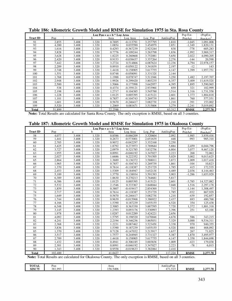
343
Table 186: Allometric Growth Model and RMSE for Simulation 1975 in Sta. Rosa County
Tract ID Log Pop = a + b * Log Area Pop Est-
PopAct
(PopEst-
PopAct)2 Pop a b Area Log Area Log_Pop AntilogPop
91 2,855 3.408 1.320 0.7695 -0.113791 3.257795 1,810 -1,045 1,091,008 92 4,200 3.408 1.320 1.0854 0.035590 3.454979 2,851 -1,349 1,820,131
93 1,616 3.408 1.320 0.4293 -0.367239 2.923244 838 -778 605,283
94 3,828 3.408 1.320 0.7776 -0.109244 3.263798 1,836 -1,992 3,969,317
95 3,628 3.408 1.320 1.8225 0.260668 3.752081 5,650 2,022 4,090,205
96 2,420 3.408 1.320 0.9153 -0.038437 3.357264 2,276 -144 20,598
97 7,442 3.408 1.320 3.2724 0.514866 4.087624 12,236 4,794 22,978,157
98 2,209 3.408 1.320 0.8910 -0.050122 3.341839 2,197 -12 143
99 2,748 3.408 1.320 1.4418 0.158905 3.617755 4,147 1,399 1,957,751
100 1,551 3.408 1.320 0.8748 -0.058091 3.331320 2,144
101 1,768 3.408 1.320 1.1988 0.078747 3.511946 3,250 1,482 2,197,707
102 2,948 3.408 1.320 1.9926 0.299420 3.803235 6,357 3,409 11,619,520
103 2,500 3.408 1.320 1.5066 0.177998 3.642957 4,395 1,895 3,590,965
104 538 3.408 1.320 0.4374 -0.359121 2.933960 859 321 102,999
105 2,198 3.408 1.320 1.2717 0.104385 3.545788 3,514 1,316 1,731,558
106 1,228 3.408 1.320 1.0125 0.005395 3.415121 2,601 1,373 1,884,818
107 1,101 3.408 1.320 0.7857 -0.104743 3.269739 1,861 760 577,551
108 1,601 3.408 1.320 0.5670 -0.246417 3.082730 1,210 -391 153,002
109 5,520 3.408 1.320 1.2069 0.081671 3.515806 3,279 -2,241 5,019,892
Total 51,899 22.2588 63,312 RMSE 2,277.78
Note: Total Results are calculated for Santa Rosa County. The only exception is RMSE, based on all 3 counties.
Table 187: Allometric Growth Model and RMSE for Simulation 1975 in Okaloosa County
Tract ID Log Pop = a + b * Log Area Pop Est-
PopAct
(PopEst-
PopAct)2 Pop a b Area Log Area Log_Pop AntilogPop
58 4,077 3.408 1.320 0.8586 -0.066209 3.320604 2,092 -1,985 3,939,416 59 1,441 3.408 1.320 0.2673 -0.573001 2.651639 448 -993 985,310
60 2,705 3.408 1.320 0.9072 -0.042297 3.352168 2,250
61 3,425 3.408 1.320 1.8792 0.273973 3.769644 5,884 2,459 6,044,796
62 3,727 3.408 1.320 2.0979 0.321785 3.832756 6,804 3,077 9,467,120
63 1,955 3.408 1.320 0.8991 -0.046192 3.347027 2,223 268 72,063
64 2,027 3.408 1.320 1.6686 0.222352 3.701505 5,029 3,002 9,013,625
65 2,864 3.408 1.320 1.3689 0.136372 3.588011 3,873 1,009 1,017,418
66 1,965 3.408 1.320 0.7857 -0.104743 3.269739 1,861 -104 10,823
67 1,370 3.408 1.320 0.7614 -0.118387 3.251729 1,785 415 172,535
68 2,453 3.408 1.320 1.5309 0.184947 3.652130 4,489 2,036 4,144,463
69 5,189 3.408 1.320 1.3770 0.138934 3.591393 3,903 -1,286 1,653,929
70 6,389 3.408 1.320 1.8630 0.270213 3.764681 5,817
71 6,386 3.408 1.320 1.0125 0.005395 3.415121 2,601 -3,785 14,327,082
72 5,532 3.408 1.320 2.1546 0.333367 3.848044 7,048 1,516 2,297,178
73 1,859 3.408 1.320 0.3807 -0.419417 2.854369 715 -1,144 1,308,497
74 2,717 3.408 1.320 0.7614 -0.118387 3.251729 1,785 -932 867,929
75 1,649 3.408 1.320 0.5670 -0.246417 3.082730 1,210 -439 192,857
76 1,744 3.408 1.320 0.9639 -0.015968 3.386922 2,437 693 480,768
77 4,166 3.408 1.320 1.5390 0.187239 3.655155 4,520 354 125,438
78 6,348 3.408 1.320 2.3085 0.363330 3.887595 7,720 1,372 1,881,318
79 3,145 3.408 1.320 1.2393 0.093176 3.530993 3,396 251 63,100
80 1,978 3.408 1.320 1.0287 0.012289 3.424221 2,656
81 4,092 3.408 1.320 1.5795 0.198520 3.670046 4,678 586 343,215
82 4,241 3.408 1.320 2.2194 0.346236 3.865031 7,329 3,088 9,534,311
83 2,368 3.408 1.320 1.2231 0.087462 3.523450 3,338 970 940,355
84 3,836 3.408 1.320 1.5390 0.187239 3.655155 4,520 684 468,092
85 1,370 3.408 1.320 0.7128 -0.147032 3.213917 1,637 267 71,025
86 3,517 3.408 1.320 1.7577 0.244945 3.731327 5,387 1,870 3,495,977
87 2,789 3.408 1.320 1.4418 0.158905 3.617755 4,147 1,358 1,844,698
88 1,432 3.408 1.320 0.4941 -0.306185 3.003836 1,009 -423 179,038
89 2,301 3.408 1.320 0.8991 -0.046192 3.347027 2,223 -78 6,015
90 1,343 3.408 1.320 0.9558 -0.019633 3.382084 2,410
Total 102,400 41.0427 117,224 RMSE 2,277.78
Note: Total Results are calculated for Okaloosa County. The only exception is RMSE, based on all 3 counties.
TOTAL Pop
Area
AntilogPop SIM 75 381,993 156.5406 471,523 RMSE 2,277.78
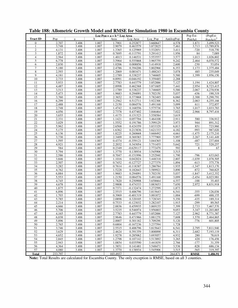
344
Table 188: Allometric Growth Model and RMSE for Simulation 1980 in Escambia County
Tract ID Log Pop = a + b * Log Area Pop Est-
PopAct
(PopEst-
PopAct)2 Pop a b Area Log Area Log_Pop AntilogPop
0 2,707 3.406 1.007 1.7901 0.252877 3.660647 4,578 1,871 3,499,523 1 3,748 3.406 1.007 2.9079 0.463579 3.872825 7,461 3,713 13,789,876
2 4,131 3.406 1.007 1.3365 0.125969 3.532851 3,411 -720 518,750
3 1,872 3.406 1.007 0.7695 -0.113791 3.291412 1,956 84 7,089
4 2,564 3.406 1.007 1.4013 0.146531 3.553557 3,577 1,013 1,026,802
5 6,778 3.406 1.007 3.5964 0.555868 3.965759 9,242 2,464 6,070,572
6 2,830 3.406 1.007 1.0206 0.008856 3.414918 2,600 -230 53,054
7 5,180 3.406 1.007 2.4786 0.394206 3.802966 6,353 1,173 1,375,484
8 2,593 3.406 1.007 1.2069 0.081671 3.488243 3,078 485 235,049
9 4,181 3.406 1.007 2.1789 0.338237 3.746605 5,580 1,399 1,956,150
10 2,733 3.406 1.007 0.8991 -0.046192 3.359485 2,288
11 5,933 3.406 1.007 2.7783 0.443779 3.852886 7,127 1,194 1,424,807
12 4,487 3.406 1.007 2.8998 0.462368 3.871605 7,441 2,954 8,723,415
13 3,513 3.406 1.007 2.1789 0.338237 3.746605 5,580 2,067 4,270,936
14 5,473 3.406 1.007 1.9683 0.294091 3.702150 5,037 -436 190,319
15 3,760 3.406 1.007 2.3652 0.373868 3.782485 6,060 2,300 5,290,791
16 6,299 3.406 1.007 3.2562 0.512711 3.922300 8,362 2,063 4,255,166
17 2,488 3.406 1.007 1.2150 0.084576 3.491168 3,099 611 372,857
18 2,748 3.406 1.007 1.4742 0.168556 3.575736 3,765 1,017 1,033,783
19 4,056 3.406 1.007 2.7378 0.437402 3.846464 7,022 2,966 8,797,416
20 3,655 3.406 1.007 1.4175 0.151523 3.558584 3,619
21 2,331 3.406 1.007 1.1421 0.057704 3.464108 2,911 580 336,912
22 3,029 3.406 1.007 1.5552 0.191786 3.599129 3,973 944 891,312
23 5,962 3.406 1.007 2.6568 0.424359 3.833329 6,813 851 723,960
24 5,175 3.406 1.007 1.6362 0.213836 3.621333 4,182 -993 987,020
25 6,136 3.406 1.007 1.8225 0.260668 3.668492 4,661 -1,475 2,175,210
26 3,730 3.406 1.007 2.3409 0.369383 3.777969 5,997 2,267 5,141,449
27 1,595 3.406 1.007 0.4374 -0.359121 3.044365 1,108 -487 237,604
28 4,921 3.406 1.007 2.2032 0.343054 3.751455 5,642 721 520,257
29 584 3.406 1.007 0.2349 -0.629117 2.772479 592 8 67
30 5,794 3.406 1.007 1.3770 0.138934 3.545906 3,515
31 2,586 3.406 1.007 0.7047 -0.151996 3.252940 1,790 -796 633,043
32 3,846 3.406 1.007 1.1016 0.042024 3.448318 2,807 -1,039 1,078,505
33 2,507 3.406 1.007 0.7452 -0.127727 3.277379 1,894 -613 375,776
34 3,282 3.406 1.007 0.7614 -0.118387 3.286784 1,935 -1,347 1,813,170
35 4,762 3.406 1.007 1.5228 0.182643 3.589921 3,890 -872 760,825
36 6,884 3.406 1.007 1.9683 0.294091 3.702150 5,037 -1,847 3,412,352
37 5,553 3.406 1.007 1.2150 0.084576 3.491168 3,099 -2,454 6,023,981
38 4,745 3.406 1.007 1.7820 0.250908 3.658664 4,557 -188 35,403
39 4,678 3.406 1.007 2.9808 0.474333 3.883653 7,650 2,972 8,831,918
40 1,875 3.406 1.007 0.7371 -0.132474 3.272599 1,873
41 6,896 3.406 1.007 2.5515 0.406796 3.815643 6,541 -355 126,036
42 1,703 3.406 1.007 0.3969 -0.401319 3.001872 1,004 -699 488,155
43 5,785 3.406 1.007 2.0898 0.320105 3.728345 5,350 -435 189,314
44 2,214 3.406 1.007 0.7533 -0.123032 3.282107 1,915 -299 89,565
45 4,666 3.406 1.007 2.8836 0.459935 3.869155 7,399 2,733 7,467,570
46 5,706 3.406 1.007 3.5235 0.546974 3.956803 9,053 3,347 11,203,885
47 4,165 3.406 1.007 2.7783 0.443779 3.852886 7,127 2,962 8,771,387
48 6,038 3.406 1.007 2.9646 0.471966 3.881270 7,608 1,570 2,464,865
49 5,896 3.406 1.007 2.0007 0.301182 3.709290 5,120 -776 601,805
50 2,765 3.406 1.007 0.6804 -0.167236 3.237594 1,728
51 3,746 3.406 1.007 2.5515 0.406796 3.815643 6,541 2,795 7,811,940
52 3,629 3.406 1.007 2.4624 0.391359 3.800098 6,311 2,682 7,193,119
53 4,652 3.406 1.007 1.9278 0.285062 3.693057 4,932 280 78,619
54 2,845 3.406 1.007 1.2798 0.107142 3.513892 3,265 420 176,456
55 2,943 3.406 1.007 1.0854 0.035590 3.441839 2,766 -177 31,359
56 4,364 3.406 1.007 1.3851 0.141481 3.548471 3,536 -828 686,134
57 4,080 3.406 1.007 1.3770 0.138934 3.545906 3,515 -565 319,397
Total 233,797 103.4937 264,871 RMSE 1,486.91
Note: Total Results are calculated for Escambia County. The only exception is RMSE, based on all 3 counties.
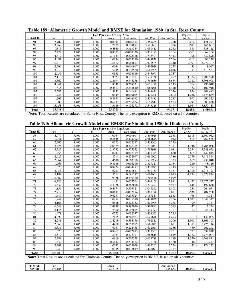
345
Table 189: Allometric Growth Model and RMSE for Simulation 1980 in Sta. Rosa County
Tract ID Log Pop = a + b * Log Area Pop Est-
PopAct
(PopEst-
PopAct)2 Pop a b Area Log Area Log_Pop AntilogPop
91 2,702 3.406 1.007 0.8991 -0.046192 3.359485 2,288 -414 171,271 92 3,969 3.406 1.007 1.2879 0.109882 3.516651 3,286 -683 466,657
93 1,813 3.406 1.007 0.4860 -0.313364 3.090443 1,232 -581 338,115
94 2,427 3.406 1.007 0.8505 -0.070326 3.335182 2,164 -263 69,366
95 4,617 3.406 1.007 2.1141 0.325126 3.733401 5,413 796 632,890
96 3,081 3.406 1.007 1.0854 0.035590 3.441839 2,766 -315 99,278
97 6,413 3.406 1.007 3.6612 0.563623 3.973569 9,410 2,997 8,979,307
98 2,590 3.406 1.007 1.0044 0.001907 3.407920 2,558 -32 1,017
99 3,319 3.406 1.007 1.5795 0.198520 3.605909 4,036 717 513,531
100 2,039 3.406 1.007 1.0935 0.038819 3.445091 2,787
101 2,118 3.406 1.007 1.3527 0.131201 3.538120 3,452 1,334 1,780,598
102 3,362 3.406 1.007 2.2194 0.346236 3.754659 5,684 2,322 5,391,998
103 4,041 3.406 1.007 1.8549 0.268321 3.676199 4,745 704 495,040
104 838 3.406 1.007 0.4617 -0.335640 3.068010 1,170 332 109,910
105 2,582 3.406 1.007 1.3851 0.141481 3.548471 3,536 954 909,483
106 1,446 3.406 1.007 1.0449 0.019075 3.425208 2,662 1,216 1,478,659
107 1,293 3.406 1.007 0.8991 -0.046192 3.359485 2,288 995 990,325
108 1,880 3.406 1.007 0.6237 -0.205024 3.199541 1,583 -297 88,080
109 5,458 3.406 1.007 1.3689 0.136372 3.543326 3,494 -1,964 3,857,188
Total 55,988 25.2720 64,551 RMSE 1,486.91
Note: Total Results are calculated for Santa Rosa County. The only exception is RMSE, based on all 3 counties.
Table 190: Allometric Growth Model and RMSE for Simulation 1980 in Okaloosa County
Tract ID Log Pop = a + b * Log Area Pop Est-
PopAct
(PopEst-
PopAct)2 Pop a b Area Log Area Log_Pop AntilogPop
58 4,077 3.406 1.007 1.0044 0.001907 3.407920 2,558 -1,519 2,307,012 59 1,441 3.406 1.007 0.3645 -0.438302 2.964629 922 -519 269,585
60 2,705 3.406 1.007 1.0773 0.032337 3.438563 2,745
61 3,425 3.406 1.007 2.0979 0.321785 3.730037 5,371 1,946 3,786,056
62 3,727 3.406 1.007 2.3733 0.375353 3.783980 6,081 2,354 5,541,652
63 1,955 3.406 1.007 1.0287 0.012289 3.418375 2,620 665 442,815
64 2,027 3.406 1.007 1.8711 0.272097 3.680002 4,786 2,759 7,613,844
65 2,864 3.406 1.007 1.4580 0.163758 3.570904 3,723 859 738,040
66 1,965 3.406 1.007 0.8586 -0.066209 3.339327 2,184 219 48,126
67 1,370 3.406 1.007 0.8424 -0.074482 3.330997 2,143 773 597,337
68 2,453 3.406 1.007 1.6281 0.211681 3.619163 4,161 1,708 2,916,123
69 5,189 3.406 1.007 1.5714 0.196287 3.603661 4,015 -1,174 1,378,814
70 6,389 3.406 1.007 1.9926 0.299420 3.707516 5,099
71 6,386 3.406 1.007 1.1421 0.057704 3.464108 2,911 -3,475 12,072,557
72 5,532 3.406 1.007 2.3328 0.367878 3.776453 5,977 445 197,650
73 1,859 3.406 1.007 0.4374 -0.359121 3.044365 1,108 -751 564,671
74 2,717 3.406 1.007 0.8181 -0.087194 3.318196 2,081 -636 404,960
75 1,649 3.406 1.007 0.6237 -0.205024 3.199541 1,583 -66 4,327
76 1,744 3.406 1.007 1.0854 0.035590 3.441839 2,766 1,022 1,044,312
77 4,166 3.406 1.007 1.6686 0.222352 3.629909 4,265 99 9,781
78 6,348 3.406 1.007 2.4948 0.397036 3.805815 6,395 47 2,174
79 3,145 3.406 1.007 1.2960 0.112605 3.519393 3,307 162 26,143
80 1,978 3.406 1.007 1.0773 0.032337 3.438563 2,745
81 4,092 3.406 1.007 1.7415 0.240923 3.648610 4,453 361 130,005
82 4,241 3.406 1.007 2.4219 0.384156 3.792845 6,206 1,965 3,863,108
83 2,368 3.406 1.007 1.4418 0.158905 3.566017 3,681 1,313 1,725,116
84 3,836 3.406 1.007 1.6767 0.224455 3.632027 4,286 450 202,273
85 1,370 3.406 1.007 0.8262 -0.082915 3.322505 2,101 731 534,918
86 3,517 3.406 1.007 1.8954 0.277701 3.685645 4,849 1,332 1,774,004
87 2,789 3.406 1.007 1.6119 0.207338 3.614789 4,119 1,330 1,768,841
88 1,432 3.406 1.007 0.5832 -0.234182 3.170178 1,480 48 2,277
89 2,301 3.406 1.007 1.0692 0.029059 3.435262 2,724 423 179,222
90 1,343 3.406 1.007 1.0935 0.038819 3.445091 2,787
Total 102,400 45.5058 116,232 RMSE 1,486.91
Note: Total Results are calculated for Okaloosa County. The only exception is RMSE, based on all 3 counties.
TOTAL Pop
Area
AntilogPop SIM 80 392,185 174.2715 445,654 RMSE 1,486.91
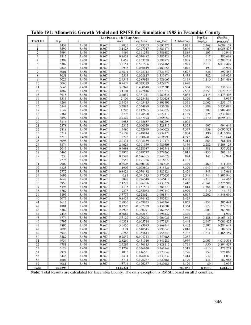
346
Table 191: Allometric Growth Model and RMSE for Simulation 1985 in Escambia County
Tract ID Log Pop = a + b * Log Area Pop Est-
PopAct
(PopEst-
PopAct)2 Pop a b Area Log Area Log_Pop AntilogPop
0 2457 3.450 0.867 1.9035 0.279553 3.692372 4,925 2,468 6,089,127 1 3599 3.450 0.867 3.1428 0.497317 3.881174 7,606 4,007 16,058,477
2 3994 3.450 0.867 1.4499 0.161338 3.589880 3,889 -105 10,946
3 1812 3.450 0.867 0.8424 -0.074482 3.385424 2,429 617 380,668
4 2398 3.450 0.867 1.458 0.163758 3.591978 3,908 1,510 2,280,731
5 6387 3.450 0.867 3.8151 0.581506 3.954166 8,998 2,611 6,819,447
6 2848 3.450 0.867 1.0935 0.038819 3.483656 3,045 197 38,999
7 6001 3.450 0.867 2.6811 0.428313 3.821347 6,627 626 392,457
8 3051 3.450 0.867 1.2555 0.098817 3.535674 3,433 382 145,926
9 5023 3.450 0.867 2.4543 0.389928 3.788067 6,139 1,116 1,244,498
10 3060 3.450 0.867 0.9477 -0.023329 3.429774 2,690
11 6646 3.450 0.867 3.0942 0.490548 3.875305 7,504 858 736,538
12 4887 3.450 0.867 3.1104 0.492816 3.877272 7,538 2,651 7,029,232
13 3918 3.450 0.867 2.4057 0.381241 3.780536 6,033 2,115 4,473,403
14 5313 3.450 0.867 2.106 0.323458 3.730438 5,376 63 3,937
15 4269 3.450 0.867 2.5434 0.405415 3.801495 6,331 2,062 4,253,179
16 6544 3.450 0.867 3.5883 0.554889 3.931089 8,533 1,989 3,955,089
17 2147 3.450 0.867 1.296 0.112605 3.547629 3,529 1,382 1,909,405
18 2364 3.450 0.867 1.5795 0.198520 3.622117 4,189 1,825 3,330,842
19 3892 3.450 0.867 2.9322 0.467194 3.855057 7,162 3,270 10,695,330
20 3316 3.450 0.867 1.4985 0.175657 3.602294 4,002
21 2378 3.450 0.867 1.2312 0.090329 3.528315 3,375 997 994,646
22 2818 3.450 0.867 1.7496 0.242939 3.660628 4,577 1,759 3,095,824
23 5714 3.450 0.867 2.8107 0.448814 3.839122 6,904 1,190 1,416,909
24 5210 3.450 0.867 1.8225 0.260668 3.675999 4,742 -468 218,644
25 6098 3.450 0.867 2.0331 0.308159 3.717174 5,214 -884 781,401
26 3874 3.450 0.867 2.4624 0.391359 3.789308 6,156 2,282 5,208,125
27 2045 3.450 0.867 0.4698 -0.328087 3.165549 1,464 -581 337,532
28 6465 3.450 0.867 2.3976 0.379777 3.779266 6,015 -450 202,116
29 733 3.450 0.867 0.2592 -0.586365 2.941622 874 141 19,944
30 7276 3.450 0.867 1.5552 0.191786 3.616279 4,133
31 2909 3.450 0.867 0.8505 -0.070326 3.389028 2,449 -460 211,398
32 4328 3.450 0.867 1.1907 0.075802 3.515721 3,279 -1,049 1,100,730
33 2772 3.450 0.867 0.8424 -0.074482 3.385424 2,429 -343 117,661
34 3692 3.450 0.867 0.81 -0.091515 3.370657 2,348 -1,344 1,806,940
35 4648 3.450 0.867 1.6848 0.226548 3.646417 4,430 -218 47,463
36 6953 3.450 0.867 2.1222 0.326786 3.733324 5,412 -1,541 2,375,989
37 5398 3.450 0.867 1.4175 0.151523 3.581370 3,814 -1,584 2,509,339
38 4769 3.450 0.867 1.9278 0.285062 3.697149 4,979 210 44,132
39 5895 3.450 0.867 3.3777 0.528621 3.908314 8,097 2,202 4,848,010
40 2073 3.450 0.867 0.8424 -0.074482 3.385424 2,429
41 7612 3.450 0.867 2.8836 0.459935 3.848764 7,059 -553 305,441
42 1881 3.450 0.867 0.4293 -0.367239 3.131604 1,354 -527 277,778
43 6389 3.450 0.867 2.2923 0.360271 3.762355 5,786 -603 363,980
44 2446 3.450 0.867 0.8667 -0.062131 3.396132 2,490 44 1,902
45 4774 3.450 0.867 3.3129 0.520208 3.901021 7,962 3,188 10,163,162
46 6797 3.450 0.867 4.0338 0.605714 3.975154 9,444 2,647 7,006,422
47 4895 3.450 0.867 3.0456 0.483673 3.869344 7,402 2,507 6,284,647
48 7096 3.450 0.867 3.24 0.510545 3.892643 7,810 714 509,577
49 6943 3.450 0.867 2.268 0.355643 3.758343 5,732 -1,211 1,465,359
50 3589 3.450 0.867 0.7857 -0.104743 3.359188 2,287
51 4934 3.450 0.867 2.8269 0.451310 3.841286 6,939 2,005 4,019,338
52 4781 3.450 0.867 2.7297 0.436115 3.828112 6,731 1,950 3,804,437
53 6129 3.450 0.867 2.1708 0.336620 3.741849 5,519 -610 372,271
54 2924 3.450 0.867 1.4013 0.146531 3.577042 3,776 852 726,060
55 3446 3.450 0.867 1.2474 0.096006 3.533237 3,414 -32 1,037
56 4604 3.450 0.867 1.5714 0.196287 3.620181 4,170 -434 187,985
57 4081 3.450 0.867 1.5714 0.196287 3.620181 4,170 89 7,997
Total 253,295 113.7321 289,055 RMSE 1,414.76
Note: Total Results are calculated for Escambia County. The only exception is RMSE, based on all 3 counties.
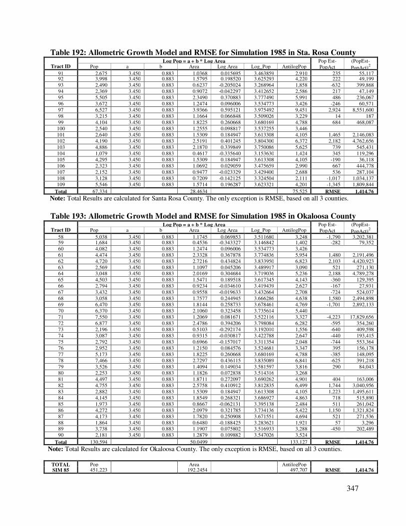
347
Table 192: Allometric Growth Model and RMSE for Simulation 1985 in Sta. Rosa County
Tract ID Log Pop = a + b * Log Area Pop Est-
PopAct
(PopEst-
PopAct)2 Pop a b Area Log Area Log_Pop AntilogPop
91 2,675 3.450 0.883 1.0368 0.015695 3.463859 2,910 235 55,117 92 3,998 3.450 0.883 1.5795 0.198520 3.625293 4,220 222 49,199
93 2,490 3.450 0.883 0.6237 -0.205024 3.268964 1,858 -632 399,868
94 2,369 3.450 0.883 0.9072 -0.042297 3.412652 2,586 217 47,149
95 5,505 3.450 0.883 2.3490 0.370883 3.777490 5,991 486 236,067
96 3,672 3.450 0.883 1.2474 0.096006 3.534773 3,426 -246 60,571
97 6,527 3.450 0.883 3.9366 0.595121 3.975492 9,451 2,924 8,551,600
98 3,215 3.450 0.883 1.1664 0.066848 3.509026 3,229 14 187
99 4,104 3.450 0.883 1.8225 0.260668 3.680169 4,788 684 468,087
100 2,540 3.450 0.883 1.2555 0.098817 3.537255 3,446
101 2,640 3.450 0.883 1.5309 0.184947 3.613308 4,105 1,465 2,146,083
102 4,190 3.450 0.883 2.5191 0.401245 3.804300 6,372 2,182 4,762,656
103 4,886 3.450 0.883 2.1870 0.339849 3.750086 5,625 739 545,431
104 1,079 3.450 0.883 0.4617 -0.335640 3.153630 1,424 345 119,296
105 4,295 3.450 0.883 1.5309 0.184947 3.613308 4,105 -190 36,118
106 2,323 3.450 0.883 1.0692 0.029059 3.475659 2,990 667 444,778
107 2,152 3.450 0.883 0.9477 -0.023329 3.429400 2,688 536 287,104
108 3,128 3.450 0.883 0.7209 -0.142125 3.324504 2,111 -1,017 1,034,137
109 5,546 3.450 0.883 1.5714 0.196287 3.623321 4,201 -1,345 1,809,844
Total 67,334 28.4634 75,525 RMSE 1,414.76
Note: Total Results are calculated for Santa Rosa County. The only exception is RMSE, based on all 3 counties.
Table 193: Allometric Growth Model and RMSE for Simulation 1985 in Okaloosa County
Tract ID Log Pop = a + b * Log Area Pop Est-
PopAct
(PopEst-
PopAct)2 Pop a b Area Log Area Log_Pop AntilogPop
58 5,038 3.450 0.883 1.1745 0.069853 3.511680 3,248 -1,790 3,202,381 59 1,684 3.450 0.883 0.4536 -0.343327 3.146842 1,402 -282 79,352
60 4,082 3.450 0.883 1.2474 0.096006 3.534773 3,426
61 4,474 3.450 0.883 2.3328 0.367878 3.774836 5,954 1,480 2,191,496
62 4,720 3.450 0.883 2.7216 0.434824 3.833950 6,823 2,103 4,420,923
63 2,569 3.450 0.883 1.1097 0.045206 3.489917 3,090 521 271,130
64 3,048 3.450 0.883 2.0169 0.304684 3.719036 5,236 2,188 4,789,278
65 4,503 3.450 0.883 1.5471 0.189518 3.617345 4,143 -360 129,395
66 2,794 3.450 0.883 0.9234 -0.034610 3.419439 2,627 -167 27,931
67 3,432 3.450 0.883 0.9558 -0.019633 3.432664 2,708 -724 524,037
68 3,058 3.450 0.883 1.7577 0.244945 3.666286 4,638 1,580 2,494,898
69 6,470 3.450 0.883 1.8144 0.258733 3.678461 4,769 -1,701 2,892,133
70 6,370 3.450 0.883 2.1060 0.323458 3.735614 5,440
71 7,550 3.450 0.883 1.2069 0.081671 3.522116 3,327 -4,223 17,829,656
72 6,877 3.450 0.883 2.4786 0.394206 3.798084 6,282 -595 354,260
73 2,196 3.450 0.883 0.5103 -0.292174 3.192010 1,556 -640 409,598
74 3,087 3.450 0.883 0.9315 -0.030817 3.422788 2,647 -440 193,415
75 2,792 3.450 0.883 0.6966 -0.157017 3.311354 2,048 -744 553,364
76 2,952 3.450 0.883 1.2150 0.084576 3.524681 3,347 395 156,178
77 5,173 3.450 0.883 1.8225 0.260668 3.680169 4,788 -385 148,095
78 7,466 3.450 0.883 2.7297 0.436115 3.835089 6,841 -625 391,218
79 3,526 3.450 0.883 1.4094 0.149034 3.581597 3,816 290 84,043
80 2,253 3.450 0.883 1.1826 0.072838 3.514316 3,268
81 4,497 3.450 0.883 1.8711 0.272097 3.690262 4,901 404 163,006
82 4,755 3.450 0.883 2.5758 0.410912 3.812835 6,499 1,744 3,040,956
83 2,882 3.450 0.883 1.5309 0.184947 3.613308 4,105 1,223 1,495,611
84 4,145 3.450 0.883 1.8549 0.268321 3.686927 4,863 718 515,890
85 1,973 3.450 0.883 0.8667 -0.062131 3.395138 2,484 511 261,042
86 4,272 3.450 0.883 2.0979 0.321785 3.734136 5,422 1,150 1,321,824
87 4,173 3.450 0.883 1.7820 0.250908 3.671551 4,694 521 271,536
88 1,864 3.450 0.883 0.6480 -0.188425 3.283621 1,921 57 3,296
89 3,738 3.450 0.883 1.1907 0.075802 3.516933 3,288 -450 202,489
90 2,181 3.450 0.883 1.2879 0.109882 3.547026 3,524
Total 130,594 50.0499 133,127 RMSE 1,414.76
Note: Total Results are calculated for Okaloosa County. The only exception is RMSE, based on all 3 counties.
TOTAL Pop
Area
AntilogPop SIM 85 451,223 192.2454 497,707 RMSE 1,414.76
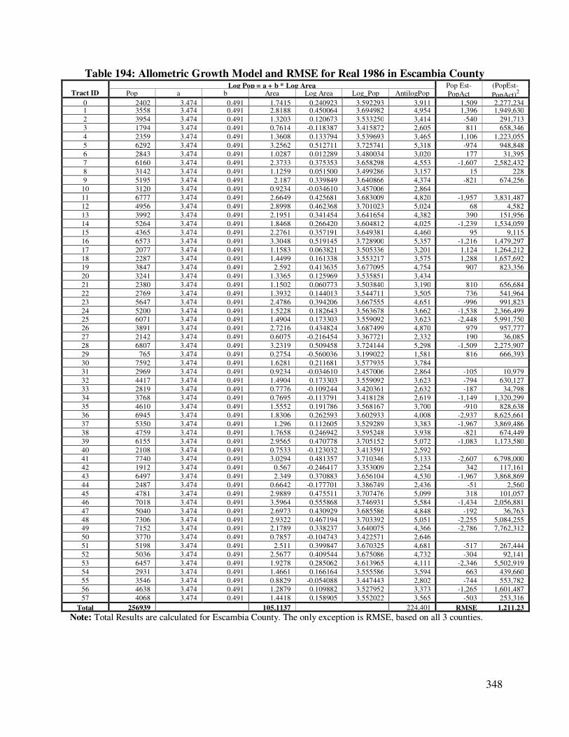
348
Table 194: Allometric Growth Model and RMSE for Real 1986 in Escambia County
Tract ID Log Pop = a + b * Log Area Pop Est-
PopAct
(PopEst-
PopAct)2 Pop a b Area Log Area Log_Pop AntilogPop
0 2402 3.474 0.491 1.7415 0.240923 3.592293 3,911 1,509 2,277,234 1 3558 3.474 0.491 2.8188 0.450064 3.694982 4,954 1,396 1,949,630
2 3954 3.474 0.491 1.3203 0.120673 3.533250 3,414 -540 291,713
3 1794 3.474 0.491 0.7614 -0.118387 3.415872 2,605 811 658,346
4 2359 3.474 0.491 1.3608 0.133794 3.539693 3,465 1,106 1,223,055
5 6292 3.474 0.491 3.2562 0.512711 3.725741 5,318 -974 948,848
6 2843 3.474 0.491 1.0287 0.012289 3.480034 3,020 177 31,395
7 6160 3.474 0.491 2.3733 0.375353 3.658298 4,553 -1,607 2,582,432
8 3142 3.474 0.491 1.1259 0.051500 3.499286 3,157 15 228
9 5195 3.474 0.491 2.187 0.339849 3.640866 4,374 -821 674,256
10 3120 3.474 0.491 0.9234 -0.034610 3.457006 2,864
11 6777 3.474 0.491 2.6649 0.425681 3.683009 4,820 -1,957 3,831,487
12 4956 3.474 0.491 2.8998 0.462368 3.701023 5,024 68 4,582
13 3992 3.474 0.491 2.1951 0.341454 3.641654 4,382 390 151,956
14 5264 3.474 0.491 1.8468 0.266420 3.604812 4,025 -1,239 1,534,059
15 4365 3.474 0.491 2.2761 0.357191 3.649381 4,460 95 9,115
16 6573 3.474 0.491 3.3048 0.519145 3.728900 5,357 -1,216 1,479,297
17 2077 3.474 0.491 1.1583 0.063821 3.505336 3,201 1,124 1,264,212
18 2287 3.474 0.491 1.4499 0.161338 3.553217 3,575 1,288 1,657,692
19 3847 3.474 0.491 2.592 0.413635 3.677095 4,754 907 823,356
20 3241 3.474 0.491 1.3365 0.125969 3.535851 3,434
21 2380 3.474 0.491 1.1502 0.060773 3.503840 3,190 810 656,684
22 2769 3.474 0.491 1.3932 0.144013 3.544711 3,505 736 541,964
23 5647 3.474 0.491 2.4786 0.394206 3.667555 4,651 -996 991,823
24 5200 3.474 0.491 1.5228 0.182643 3.563678 3,662 -1,538 2,366,499
25 6071 3.474 0.491 1.4904 0.173303 3.559092 3,623 -2,448 5,991,750
26 3891 3.474 0.491 2.7216 0.434824 3.687499 4,870 979 957,777
27 2142 3.474 0.491 0.6075 -0.216454 3.367721 2,332 190 36,085
28 6807 3.474 0.491 3.2319 0.509458 3.724144 5,298 -1,509 2,275,907
29 765 3.474 0.491 0.2754 -0.560036 3.199022 1,581 816 666,393
30 7592 3.474 0.491 1.6281 0.211681 3.577935 3,784
31 2969 3.474 0.491 0.9234 -0.034610 3.457006 2,864 -105 10,979
32 4417 3.474 0.491 1.4904 0.173303 3.559092 3,623 -794 630,127
33 2819 3.474 0.491 0.7776 -0.109244 3.420361 2,632 -187 34,798
34 3768 3.474 0.491 0.7695 -0.113791 3.418128 2,619 -1,149 1,320,299
35 4610 3.474 0.491 1.5552 0.191786 3.568167 3,700 -910 828,638
36 6945 3.474 0.491 1.8306 0.262593 3.602933 4,008 -2,937 8,625,661
37 5350 3.474 0.491 1.296 0.112605 3.529289 3,383 -1,967 3,869,486
38 4759 3.474 0.491 1.7658 0.246942 3.595248 3,938 -821 674,449
39 6155 3.474 0.491 2.9565 0.470778 3.705152 5,072 -1,083 1,173,580
40 2108 3.474 0.491 0.7533 -0.123032 3.413591 2,592
41 7740 3.474 0.491 3.0294 0.481357 3.710346 5,133 -2,607 6,798,000
42 1912 3.474 0.491 0.567 -0.246417 3.353009 2,254 342 117,161
43 6497 3.474 0.491 2.349 0.370883 3.656104 4,530 -1,967 3,868,869
44 2487 3.474 0.491 0.6642 -0.177701 3.386749 2,436 -51 2,560
45 4781 3.474 0.491 2.9889 0.475511 3.707476 5,099 318 101,057
46 7018 3.474 0.491 3.5964 0.555868 3.746931 5,584 -1,434 2,056,881
47 5040 3.474 0.491 2.6973 0.430929 3.685586 4,848 -192 36,763
48 7306 3.474 0.491 2.9322 0.467194 3.703392 5,051 -2,255 5,084,255
49 7152 3.474 0.491 2.1789 0.338237 3.640075 4,366 -2,786 7,762,312
50 3770 3.474 0.491 0.7857 -0.104743 3.422571 2,646
51 5198 3.474 0.491 2.511 0.399847 3.670325 4,681 -517 267,444
52 5036 3.474 0.491 2.5677 0.409544 3.675086 4,732 -304 92,141
53 6457 3.474 0.491 1.9278 0.285062 3.613965 4,111 -2,346 5,502,919
54 2931 3.474 0.491 1.4661 0.166164 3.555586 3,594 663 439,660
55 3546 3.474 0.491 0.8829 -0.054088 3.447443 2,802 -744 553,782
56 4638 3.474 0.491 1.2879 0.109882 3.527952 3,373 -1,265 1,601,487
57 4068 3.474 0.491 1.4418 0.158905 3.552022 3,565 -503 253,316
Total 256939 105.1137 224,401 RMSE 1,211.23
Note: Total Results are calculated for Escambia County. The only exception is RMSE, based on all 3 counties.
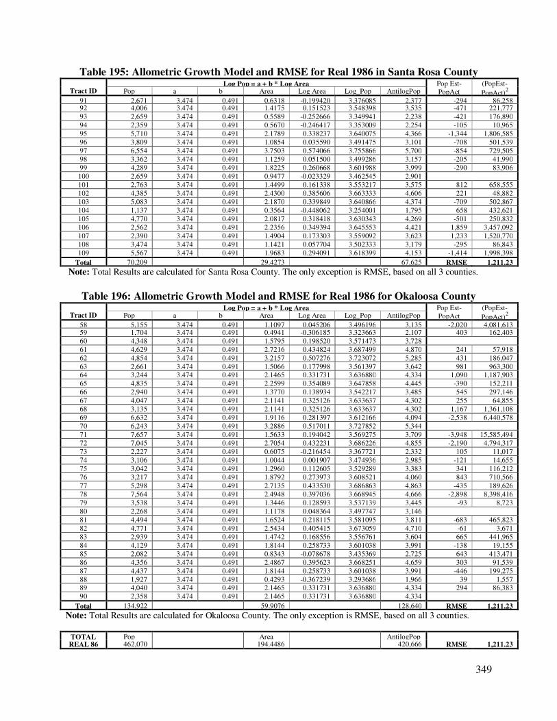
349
Table 195: Allometric Growth Model and RMSE for Real 1986 in Santa Rosa County
Tract ID Log Pop = a + b * Log Area Pop Est-
PopAct
(PopEst-
PopAct)2 Pop a b Area Log Area Log_Pop AntilogPop
91 2,671 3.474 0.491 0.6318 -0.199420 3.376085 2,377 -294 86,258 92 4,006 3.474 0.491 1.4175 0.151523 3.548398 3,535 -471 221,777
93 2,659 3.474 0.491 0.5589 -0.252666 3.349941 2,238 -421 176,890
94 2,359 3.474 0.491 0.5670 -0.246417 3.353009 2,254 -105 10,965
95 5,710 3.474 0.491 2.1789 0.338237 3.640075 4,366 -1,344 1,806,585
96 3,809 3.474 0.491 1.0854 0.035590 3.491475 3,101 -708 501,539
97 6,554 3.474 0.491 3.7503 0.574066 3.755866 5,700 -854 729,505
98 3,362 3.474 0.491 1.1259 0.051500 3.499286 3,157 -205 41,990
99 4,289 3.474 0.491 1.8225 0.260668 3.601988 3,999 -290 83,906
100 2,659 3.474 0.491 0.9477 -0.023329 3.462545 2,901
101 2,763 3.474 0.491 1.4499 0.161338 3.553217 3,575 812 658,555
102 4,385 3.474 0.491 2.4300 0.385606 3.663333 4,606 221 48,882
103 5,083 3.474 0.491 2.1870 0.339849 3.640866 4,374 -709 502,867
104 1,137 3.474 0.491 0.3564 -0.448062 3.254001 1,795 658 432,621
105 4,770 3.474 0.491 2.0817 0.318418 3.630343 4,269 -501 250,832
106 2,562 3.474 0.491 2.2356 0.349394 3.645553 4,421 1,859 3,457,092
107 2,390 3.474 0.491 1.4904 0.173303 3.559092 3,623 1,233 1,520,770
108 3,474 3.474 0.491 1.1421 0.057704 3.502333 3,179 -295 86,843
109 5,567 3.474 0.491 1.9683 0.294091 3.618399 4,153 -1,414 1,998,398
Total 70,209 29.4273 67,625 RMSE 1,211.23
Note: Total Results are calculated for Santa Rosa County. The only exception is RMSE, based on all 3 counties.
Table 196: Allometric Growth Model and RMSE for Real 1986 for Okaloosa County
Tract ID Log Pop = a + b * Log Area Pop Est-
PopAct
(PopEst-
PopAct)2 Pop a b Area Log Area Log_Pop AntilogPop
58 5,155 3.474 0.491 1.1097 0.045206 3.496196 3,135 -2,020 4,081,613 59 1,704 3.474 0.491 0.4941 -0.306185 3.323663 2,107 403 162,403
60 4,348 3.474 0.491 1.5795 0.198520 3.571473 3,728
61 4,629 3.474 0.491 2.7216 0.434824 3.687499 4,870 241 57,918
62 4,854 3.474 0.491 3.2157 0.507276 3.723072 5,285 431 186,047
63 2,661 3.474 0.491 1.5066 0.177998 3.561397 3,642 981 963,300
64 3,244 3.474 0.491 2.1465 0.331731 3.636880 4,334 1,090 1,187,903
65 4,835 3.474 0.491 2.2599 0.354089 3.647858 4,445 -390 152,211
66 2,940 3.474 0.491 1.3770 0.138934 3.542217 3,485 545 297,146
67 4,047 3.474 0.491 2.1141 0.325126 3.633637 4,302 255 64,855
68 3,135 3.474 0.491 2.1141 0.325126 3.633637 4,302 1,167 1,361,108
69 6,632 3.474 0.491 1.9116 0.281397 3.612166 4,094 -2,538 6,440,578
70 6,243 3.474 0.491 3.2886 0.517011 3.727852 5,344
71 7,657 3.474 0.491 1.5633 0.194042 3.569275 3,709 -3,948 15,585,494
72 7,045 3.474 0.491 2.7054 0.432231 3.686226 4,855 -2,190 4,794,317
73 2,227 3.474 0.491 0.6075 -0.216454 3.367721 2,332 105 11,017
74 3,106 3.474 0.491 1.0044 0.001907 3.474936 2,985 -121 14,655
75 3,042 3.474 0.491 1.2960 0.112605 3.529289 3,383 341 116,212
76 3,217 3.474 0.491 1.8792 0.273973 3.608521 4,060 843 710,566
77 5,298 3.474 0.491 2.7135 0.433530 3.686863 4,863 -435 189,626
78 7,564 3.474 0.491 2.4948 0.397036 3.668945 4,666 -2,898 8,398,416
79 3,538 3.474 0.491 1.3446 0.128593 3.537139 3,445 -93 8,723
80 2,268 3.474 0.491 1.1178 0.048364 3.497747 3,146
81 4,494 3.474 0.491 1.6524 0.218115 3.581095 3,811 -683 465,823
82 4,771 3.474 0.491 2.5434 0.405415 3.673059 4,710 -61 3,671
83 2,939 3.474 0.491 1.4742 0.168556 3.556761 3,604 665 441,965
84 4,129 3.474 0.491 1.8144 0.258733 3.601038 3,991 -138 19,155
85 2,082 3.474 0.491 0.8343 -0.078678 3.435369 2,725 643 413,471
86 4,356 3.474 0.491 2.4867 0.395623 3.668251 4,659 303 91,539
87 4,437 3.474 0.491 1.8144 0.258733 3.601038 3,991 -446 199,275
88 1,927 3.474 0.491 0.4293 -0.367239 3.293686 1,966 39 1,557
89 4,040 3.474 0.491 2.1465 0.331731 3.636880 4,334 294 86,383
90 2,358 3.474 0.491 2.1465 0.331731 3.636880 4,334
Total 134,922 59.9076 128,640 RMSE 1,211.23
Note: Total Results are calculated for Okaloosa County. The only exception is RMSE, based on all 3 counties.
TOTAL Pop
Area
AntilogPop REAL 86 462,070 194.4486 420,666 RMSE 1,211.23

350
Table 197: Allometric Growth Model and RMSE for Simulation 1986 in Escambia County
Tract ID Log Pop = a + b * Log Area Pop Est-
PopAct
(PopEst-
PopAct)2 Pop a b Area Log Area Log_Pop AntilogPop
0 2402 3.456 0.845 1.9035 0.279553 3.692222 4,923 2,521 6,355,004 1 3558 3.456 0.845 3.159 0.499550 3.878119 7,553 3,995 15,960,018
2 3954 3.456 0.845 1.4661 0.166164 3.596408 3,948 -6 33
3 1794 3.456 0.845 0.8505 -0.070326 3.396575 2,492 698 487,418
4 2359 3.456 0.845 1.458 0.163758 3.594375 3,930 1,571 2,467,545
5 6292 3.456 0.845 3.8556 0.586092 3.951248 8,938 2,646 7,002,118
6 2843 3.456 0.845 1.1178 0.048364 3.496868 3,140 297 87,943
7 6160 3.456 0.845 2.7216 0.434824 3.823427 6,659 499 249,269
8 3142 3.456 0.845 1.296 0.112605 3.551151 3,558 416 172,683
9 5195 3.456 0.845 2.4948 0.397036 3.791495 6,187 992 984,490
10 3120 3.456 0.845 0.9558 -0.019633 3.439410 2,750
11 6777 3.456 0.845 3.1347 0.496196 3.875286 7,504 727 528,348
12 4956 3.456 0.845 3.1347 0.496196 3.875286 7,504 2,548 6,491,668
13 3992 3.456 0.845 2.4543 0.389928 3.785489 6,102 2,110 4,453,088
14 5264 3.456 0.845 2.1546 0.333367 3.737695 5,466 202 40,932
15 4365 3.456 0.845 2.592 0.413635 3.805522 6,390 2,025 4,101,859
16 6573 3.456 0.845 3.6612 0.563623 3.932262 8,556 1,983 3,931,589
17 2077 3.456 0.845 1.3041 0.115311 3.553438 3,576 1,499 2,247,993
18 2287 3.456 0.845 1.5957 0.202951 3.627494 4,241 1,954 3,819,090
19 3847 3.456 0.845 3.0132 0.479028 3.860779 7,257 3,410 11,630,551
20 3241 3.456 0.845 1.5066 0.177998 3.606408 4,040
21 2380 3.456 0.845 1.2555 0.098817 3.539500 3,463 1,083 1,173,712
22 2769 3.456 0.845 1.7739 0.248929 3.666345 4,638 1,869 3,493,735
23 5647 3.456 0.845 2.8593 0.456260 3.841539 6,943 1,296 1,679,297
24 5200 3.456 0.845 1.8468 0.266420 3.681125 4,799 -401 161,031
25 6071 3.456 0.845 2.0574 0.313319 3.720754 5,257 -814 662,274
26 3891 3.456 0.845 2.511 0.399847 3.793870 6,221 2,330 5,429,586
27 2142 3.456 0.845 0.486 -0.313364 3.191208 1,553 -589 346,769
28 6807 3.456 0.845 2.4786 0.394206 3.789104 6,153 -654 427,391
29 765 3.456 0.845 0.2592 -0.586365 2.960522 913 148 21,936
30 7592 3.456 0.845 1.5876 0.200741 3.625626 4,223
31 2969 3.456 0.845 0.8586 -0.066209 3.400053 2,512 -457 208,671
32 4417 3.456 0.845 1.2393 0.093176 3.534734 3,426 -991 982,914
33 2819 3.456 0.845 0.8586 -0.066209 3.400053 2,512 -307 94,129
34 3768 3.456 0.845 0.8424 -0.074482 3.393063 2,472 -1,296 1,679,401
35 4610 3.456 0.845 1.7172 0.234821 3.654424 4,513 -97 9,493
36 6945 3.456 0.845 2.1708 0.336620 3.740444 5,501 -1,444 2,085,059
37 5350 3.456 0.845 1.4418 0.158905 3.590275 3,893 -1,457 2,123,101
38 4759 3.456 0.845 1.9764 0.295875 3.706014 5,082 323 104,175
39 6155 3.456 0.845 3.4668 0.539929 3.912240 8,170 2,015 4,061,572
40 2108 3.456 0.845 0.8667 -0.062131 3.403499 2,532
41 7740 3.456 0.845 2.9241 0.465992 3.849763 7,076 -664 441,424
42 1912 3.456 0.845 0.4293 -0.367239 3.145683 1,399 -513 263,615
43 6497 3.456 0.845 2.3166 0.364851 3.764299 5,812 -685 469,710
44 2487 3.456 0.845 0.8748 -0.058091 3.406913 2,552 65 4,250
45 4781 3.456 0.845 3.4344 0.535851 3.908794 8,106 3,325 11,054,060
46 7018 3.456 0.845 4.1148 0.614349 3.975125 9,443 2,425 5,882,174
47 5040 3.456 0.845 3.0942 0.490548 3.870513 7,422 2,382 5,673,308
48 7306 3.456 0.845 3.321 0.521269 3.896472 7,879 573 328,352
49 7152 3.456 0.845 2.3085 0.363330 3.763014 5,794 -1,358 1,842,887
50 3770 3.456 0.845 0.81 -0.091515 3.378670 2,391
51 5198 3.456 0.845 2.8917 0.461153 3.845674 7,009 1,811 3,280,798
52 5036 3.456 0.845 2.7459 0.438685 3.826689 6,709 1,673 2,800,521
53 6457 3.456 0.845 2.2275 0.347818 3.749906 5,622 -835 696,898
54 2931 3.456 0.845 1.4499 0.161338 3.592331 3,911 980 961,156
55 3546 3.456 0.845 1.3122 0.118000 3.555710 3,595 49 2,410
56 4638 3.456 0.845 1.6281 0.211681 3.634871 4,314 -324 105,038
57 4068 3.456 0.845 1.6119 0.207338 3.631201 4,278 210 43,934
Total 256939 115.8786 292,806 RMSE 1,405.18
Note: Total Results are calculated for Escambia County. The only exception is RMSE, based on all 3 counties.

351
Table 198: Allometric Growth Model and RMSE for Simulation 1986 in Sta. Rosa County
Tract ID Log Pop = a + b * Log Area Pop Est-
PopAct
(PopEst-
PopAct)2 Pop a b Area Log Area Log_Pop AntilogPop
91 2,671 3.456 0.845 1.0611 0.025756 3.477764 3,004 333 111,185 92 4,006 3.456 0.845 1.6524 0.218115 3.640307 4,368 362 131,224
93 2,659 3.456 0.845 0.6885 -0.162096 3.319029 2,085 -574 329,902
94 2,359 3.456 0.845 0.9396 -0.027057 3.433137 2,711 352 123,936
95 5,710 3.456 0.845 2.4138 0.382701 3.779383 6,017 307 94,271
96 3,809 3.456 0.845 1.2636 0.101610 3.541860 3,482 -327 106,765
97 6,554 3.456 0.845 4.0014 0.602212 3.964869 9,223 2,669 7,123,210
98 3,362 3.456 0.845 1.2069 0.081671 3.525012 3,350 -12 150
99 4,289 3.456 0.845 1.8387 0.264511 3.679512 4,781 492 241,988
100 2,659 3.456 0.845 1.3122 0.118000 3.555710 3,595
101 2,763 3.456 0.845 1.5633 0.194042 3.619966 4,168 1,405 1,975,051
102 4,385 3.456 0.845 2.5515 0.406796 3.799742 6,306 1,921 3,689,588
103 5,083 3.456 0.845 2.2518 0.352530 3.753888 5,674 591 349,256
104 1,137 3.456 0.845 0.4860 -0.313364 3.191208 1,553 416 173,164
105 4,770 3.456 0.845 1.5552 0.191786 3.618059 4,150 -620 384,266
106 2,562 3.456 0.845 1.0692 0.029059 3.480555 3,024 462 213,270
107 2,390 3.456 0.845 0.9639 -0.015968 3.442507 2,770 380 144,532
108 3,474 3.456 0.845 0.7209 -0.142125 3.335904 2,167 -1,307 1,707,656
109 5,567 3.456 0.845 1.5876 0.200741 3.625626 4,223 -1,344 1,806,202
Total 70,209 29.1276 76,652 RMSE 1,405.18
Note: Total Results are calculated for Santa Rosa County. The only exception is RMSE, based on all 3 counties.
Table 199: Allometric Growth Model and RMSE for Simulation 1986 in Okaloosa County
Tract ID Log Pop = a + b * Log Area Pop Est-
PopAct
(PopEst-
PopAct)2 Pop a b Area Log Area Log_Pop AntilogPop
58 5,155 3.456 0.845 1.1826 0.072838 3.517548 3,293 -1,862 3,468,279 59 1,704 3.456 0.845 0.4698 -0.328087 3.178766 1,509 -195 37,920
60 4,348 3.456 0.845 1.2879 0.109882 3.548850 3,539
61 4,629 3.456 0.845 2.3814 0.376832 3.774423 5,949 1,320 1,741,654
62 4,854 3.456 0.845 2.8026 0.447561 3.834189 6,826 1,972 3,890,201
63 2,661 3.456 0.845 1.1421 0.057704 3.504760 3,197 536 287,433
64 3,244 3.456 0.845 2.0331 0.308159 3.716394 5,205 1,961 3,844,271
65 4,835 3.456 0.845 1.5633 0.194042 3.619966 4,168 -667 444,402
66 2,940 3.456 0.845 0.9639 -0.015968 3.442507 2,770 -170 28,841
67 4,047 3.456 0.845 0.9639 -0.015968 3.442507 2,770 -1,277 1,630,285
68 3,135 3.456 0.845 1.7739 0.248929 3.666345 4,638 1,503 2,259,470
69 6,632 3.456 0.845 1.8630 0.270213 3.684330 4,834 -1,798 3,231,875
70 6,243 3.456 0.845 2.1384 0.330089 3.734925 5,432
71 7,657 3.456 0.845 1.2150 0.084576 3.527467 3,369 -4,288 18,389,210
72 7,045 3.456 0.845 2.5272 0.402640 3.796230 6,255 -790 624,028
73 2,227 3.456 0.845 0.5346 -0.271971 3.226184 1,683 -544 295,513
74 3,106 3.456 0.845 0.9315 -0.030817 3.429960 2,691 -415 171,989
75 3,042 3.456 0.845 0.7047 -0.151996 3.327564 2,126 -916 839,053
76 3,217 3.456 0.845 1.2231 0.087462 3.529905 3,388 171 29,140
77 5,298 3.456 0.845 1.8711 0.272097 3.685922 4,852 -446 198,904
78 7,564 3.456 0.845 2.7621 0.441239 3.828847 6,743 -821 674,191
79 3,538 3.456 0.845 1.4175 0.151523 3.584037 3,837 299 89,640
80 2,268 3.456 0.845 1.2069 0.081671 3.525012 3,350
81 4,494 3.456 0.845 1.9116 0.281397 3.693780 4,941 447 199,460
82 4,771 3.456 0.845 2.6082 0.416341 3.807808 6,424 1,653 2,732,532
83 2,939 3.456 0.845 1.5552 0.191786 3.618059 4,150 1,211 1,466,782
84 4,129 3.456 0.845 1.8792 0.273973 3.687507 4,870 741 548,719
85 2,082 3.456 0.845 0.8748 -0.058091 3.406913 2,552 470 221,078
86 4,356 3.456 0.845 2.1627 0.334996 3.739072 5,484 1,128 1,271,655
87 4,437 3.456 0.845 1.8144 0.258733 3.674629 4,727 290 84,377
88 1,927 3.456 0.845 0.6723 -0.172437 3.310291 2,043 116 13,481
89 4,040 3.456 0.845 1.2231 0.087462 3.529905 3,388 -652 425,491
90 2,358 3.456 0.845 1.2960 0.112605 3.551151 3,558
Total 134,922 50.9571 134,561 RMSE 1,405.18
Note: Total Results are calculated for Okaloosa County. The only exception is RMSE, based on all 3 counties.
TOTAL Pop
Area
AntilogPop SIM 86 462,070 195.9633 504,019 RMSE 1,405.18
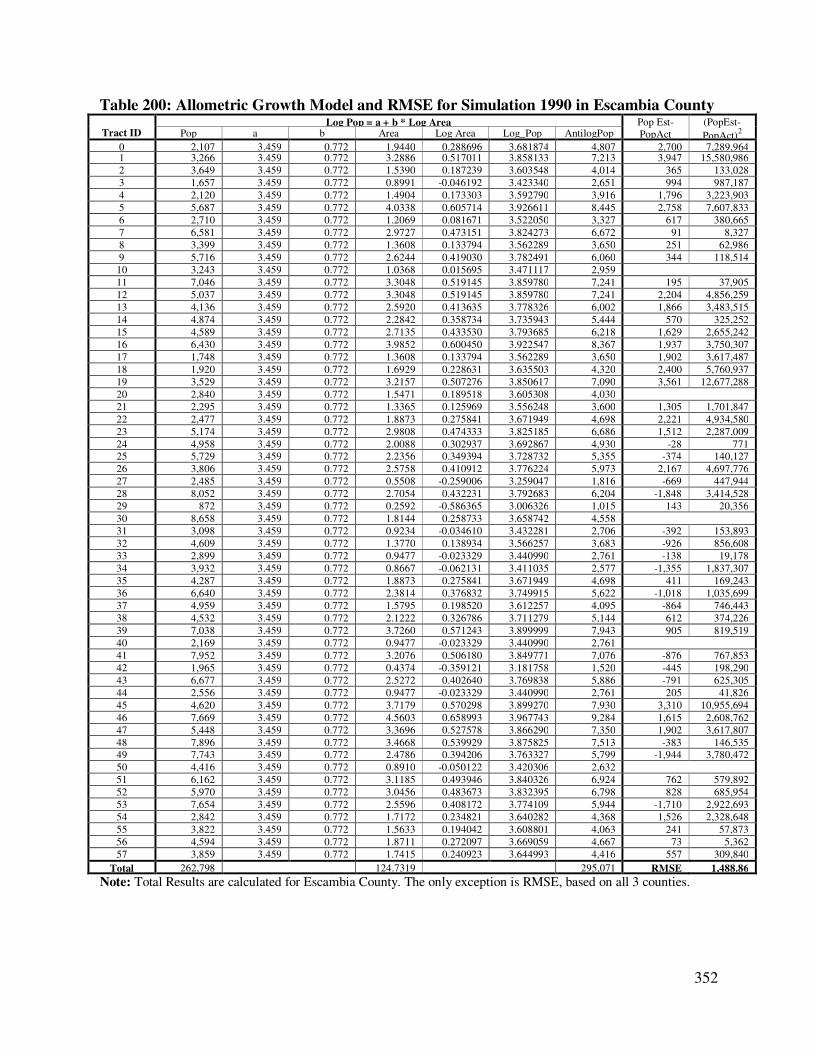
352
Table 200: Allometric Growth Model and RMSE for Simulation 1990 in Escambia County
Tract ID Log Pop = a + b * Log Area Pop Est-
PopAct
(PopEst-
PopAct)2 Pop a b Area Log Area Log_Pop AntilogPop
0 2,107 3.459 0.772 1.9440 0.288696 3.681874 4,807 2,700 7,289,964 1 3,266 3.459 0.772 3.2886 0.517011 3.858133 7,213 3,947 15,580,986
2 3,649 3.459 0.772 1.5390 0.187239 3.603548 4,014 365 133,028
3 1,657 3.459 0.772 0.8991 -0.046192 3.423340 2,651 994 987,187
4 2,120 3.459 0.772 1.4904 0.173303 3.592790 3,916 1,796 3,223,903
5 5,687 3.459 0.772 4.0338 0.605714 3.926611 8,445 2,758 7,607,833
6 2,710 3.459 0.772 1.2069 0.081671 3.522050 3,327 617 380,665
7 6,581 3.459 0.772 2.9727 0.473151 3.824273 6,672 91 8,327
8 3,399 3.459 0.772 1.3608 0.133794 3.562289 3,650 251 62,986
9 5,716 3.459 0.772 2.6244 0.419030 3.782491 6,060 344 118,514
10 3,243 3.459 0.772 1.0368 0.015695 3.471117 2,959
11 7,046 3.459 0.772 3.3048 0.519145 3.859780 7,241 195 37,905
12 5,037 3.459 0.772 3.3048 0.519145 3.859780 7,241 2,204 4,856,259
13 4,136 3.459 0.772 2.5920 0.413635 3.778326 6,002 1,866 3,483,515
14 4,874 3.459 0.772 2.2842 0.358734 3.735943 5,444 570 325,252
15 4,589 3.459 0.772 2.7135 0.433530 3.793685 6,218 1,629 2,655,242
16 6,430 3.459 0.772 3.9852 0.600450 3.922547 8,367 1,937 3,750,307
17 1,748 3.459 0.772 1.3608 0.133794 3.562289 3,650 1,902 3,617,487
18 1,920 3.459 0.772 1.6929 0.228631 3.635503 4,320 2,400 5,760,937
19 3,529 3.459 0.772 3.2157 0.507276 3.850617 7,090 3,561 12,677,288
20 2,840 3.459 0.772 1.5471 0.189518 3.605308 4,030
21 2,295 3.459 0.772 1.3365 0.125969 3.556248 3,600 1,305 1,701,847
22 2,477 3.459 0.772 1.8873 0.275841 3.671949 4,698 2,221 4,934,580
23 5,174 3.459 0.772 2.9808 0.474333 3.825185 6,686 1,512 2,287,009
24 4,958 3.459 0.772 2.0088 0.302937 3.692867 4,930 -28 771
25 5,729 3.459 0.772 2.2356 0.349394 3.728732 5,355 -374 140,127
26 3,806 3.459 0.772 2.5758 0.410912 3.776224 5,973 2,167 4,697,776
27 2,485 3.459 0.772 0.5508 -0.259006 3.259047 1,816 -669 447,944
28 8,052 3.459 0.772 2.7054 0.432231 3.792683 6,204 -1,848 3,414,528
29 872 3.459 0.772 0.2592 -0.586365 3.006326 1,015 143 20,356
30 8,658 3.459 0.772 1.8144 0.258733 3.658742 4,558
31 3,098 3.459 0.772 0.9234 -0.034610 3.432281 2,706 -392 153,893
32 4,609 3.459 0.772 1.3770 0.138934 3.566257 3,683 -926 856,608
33 2,899 3.459 0.772 0.9477 -0.023329 3.440990 2,761 -138 19,178
34 3,932 3.459 0.772 0.8667 -0.062131 3.411035 2,577 -1,355 1,837,307
35 4,287 3.459 0.772 1.8873 0.275841 3.671949 4,698 411 169,243
36 6,640 3.459 0.772 2.3814 0.376832 3.749915 5,622 -1,018 1,035,699
37 4,959 3.459 0.772 1.5795 0.198520 3.612257 4,095 -864 746,443
38 4,532 3.459 0.772 2.1222 0.326786 3.711279 5,144 612 374,226
39 7,038 3.459 0.772 3.7260 0.571243 3.899999 7,943 905 819,519
40 2,169 3.459 0.772 0.9477 -0.023329 3.440990 2,761
41 7,952 3.459 0.772 3.2076 0.506180 3.849771 7,076 -876 767,853
42 1,965 3.459 0.772 0.4374 -0.359121 3.181758 1,520 -445 198,290
43 6,677 3.459 0.772 2.5272 0.402640 3.769838 5,886 -791 625,305
44 2,556 3.459 0.772 0.9477 -0.023329 3.440990 2,761 205 41,826
45 4,620 3.459 0.772 3.7179 0.570298 3.899270 7,930 3,310 10,955,694
46 7,669 3.459 0.772 4.5603 0.658993 3.967743 9,284 1,615 2,608,762
47 5,448 3.459 0.772 3.3696 0.527578 3.866290 7,350 1,902 3,617,807
48 7,896 3.459 0.772 3.4668 0.539929 3.875825 7,513 -383 146,535
49 7,743 3.459 0.772 2.4786 0.394206 3.763327 5,799 -1,944 3,780,472
50 4,416 3.459 0.772 0.8910 -0.050122 3.420306 2,632
51 6,162 3.459 0.772 3.1185 0.493946 3.840326 6,924 762 579,892
52 5,970 3.459 0.772 3.0456 0.483673 3.832395 6,798 828 685,954
53 7,654 3.459 0.772 2.5596 0.408172 3.774109 5,944 -1,710 2,922,693
54 2,842 3.459 0.772 1.7172 0.234821 3.640282 4,368 1,526 2,328,648
55 3,822 3.459 0.772 1.5633 0.194042 3.608801 4,063 241 57,873
56 4,594 3.459 0.772 1.8711 0.272097 3.669059 4,667 73 5,362
57 3,859 3.459 0.772 1.7415 0.240923 3.644993 4,416 557 309,840
Total 262,798 124.7319 295,071 RMSE 1,488.86
Note: Total Results are calculated for Escambia County. The only exception is RMSE, based on all 3 counties.
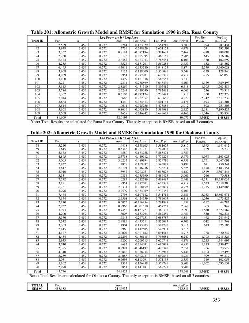
353
Table 201: Allometric Growth Model and RMSE for Simulation 1990 in Sta. Rosa County
Tract ID Log Pop = a + b * Log Area Pop Est-
PopAct
(PopEst-
PopAct)2 Pop a b Area Log Area Log_Pop AntilogPop
91 2,589 3.459 0.772 1.3284 0.123329 3.554210 3,583 994 987,431 92 3,938 3.459 0.772 1.7739 0.248929 3.651173 4,479 541 292,594
93 3,352 3.459 0.772 0.8181 -0.087194 3.391687 2,464 -888 788,082
94 2,260 3.459 0.772 1.0125 0.005395 3.463165 2,905 645 416,187
95 6,424 3.459 0.772 2.6487 0.423033 3.785581 6,104 -320 102,699
96 4,285 3.459 0.772 1.3527 0.131201 3.560288 3,633 -652 424,862
97 6,495 3.459 0.772 4.3011 0.633580 3.948123 8,874 2,379 5,660,028
98 3,908 3.459 0.772 1.3122 0.118000 3.550096 3,549 -359 128,940
99 4,969 3.459 0.772 1.8954 0.277701 3.673385 4,714 -255 65,050
100 3,100 3.459 0.772 1.4499 0.161338 3.583553 3,833
101 3,221 3.459 0.772 1.7334 0.238899 3.643430 4,400 1,179 1,389,496
102 5,113 3.459 0.772 2.8269 0.451310 3.807412 6,418 1,305 1,703,486
103 5,784 3.459 0.772 2.6244 0.419030 3.782491 6,060 276 76,319
104 1,362 3.459 0.772 0.5103 -0.292174 3.233441 1,712 350 122,328
105 7,014 3.459 0.772 1.6686 0.222352 3.630656 4,272 -2,742 7,517,232
106 3,664 3.459 0.772 1.1340 0.054613 3.501161 3,171 -493 243,301
107 3,514 3.459 0.772 1.0611 0.025756 3.478884 3,012 -502 251,803
108 5,108 3.459 0.772 0.8019 -0.095880 3.384981 2,427 -2,681 7,190,427
109 5,509 3.459 0.772 1.7658 0.246942 3.649639 4,463 -1,046 1,093,859
Total 81,609 32.0193 80,073 RMSE 1,488.86
Note: Total Results are calculated for Santa Rosa County. The only exception is RMSE, based on all 3 counties.
Table 202: Allometric Growth Model and RMSE for Simulation 1990 for Okaloosa County
Tract ID Log Pop = a + b * Log Area Pop Est-
PopAct
(PopEst-
PopAct)2 Pop a b Area Log Area Log_Pop AntilogPop
58 5,210 3.459 0.772 1.4418 0.158905 3.581675 3,817 -1,393 1,941,612 59 1,645 3.459 0.772 0.5346 -0.271971 3.249038 1,774 129 16,730
60 5,172 3.459 0.772 1.4580 0.163758 3.585421 3,850
61 4,895 3.459 0.772 2.5758 0.410912 3.776224 5,973 1,078 1,163,023
62 5,005 3.459 0.772 3.0213 0.480194 3.829710 6,756 1,751 3,067,091
63 2,827 3.459 0.772 1.2879 0.109882 3.543829 3,498 671 450,341
64 3,847 3.459 0.772 2.2194 0.346236 3.726294 5,325 1,478 2,183,551
65 5,946 3.459 0.772 1.5957 0.202951 3.615678 4,127 -1,819 3,307,244
66 3,331 3.459 0.772 1.0854 0.035590 3.486475 3,065 -266 70,588
67 7,272 3.459 0.772 1.0287 0.012289 3.468487 2,941 -4,331 18,758,037
68 3,191 3.459 0.772 1.8954 0.277701 3.673385 4,714 1,523 2,319,380
69 6,751 3.459 0.772 2.0331 0.308159 3.696899 4,976 -1,775 3,149,886
70 5,296 3.459 0.772 2.2599 0.354089 3.732357 5,400
71 7,464 3.459 0.772 1.2798 0.107142 3.541714 3,481 -3,983 15,863,671
72 7,154 3.459 0.772 2.6568 0.424359 3.786605 6,118 -1,036 1,073,425
73 2,170 3.459 0.772 0.6075 -0.216454 3.291898 1,958 -212 44,782
74 2,932 3.459 0.772 0.9963 -0.001610 3.457757 2,869 -63 3,947
75 3,973 3.459 0.772 0.7452 -0.127727 3.360395 2,293 -1,680 2,822,567
76 4,200 3.459 0.772 1.3608 0.133794 3.562289 3,650 -550 302,534
77 5,376 3.459 0.772 1.9845 0.297651 3.688787 4,884 -492 241,942
78 7,342 3.459 0.772 2.9889 0.475511 3.826095 6,700 -642 411,768
79 3,303 3.459 0.772 1.4904 0.173303 3.592790 3,916 613 375,185
80 2,145 3.459 0.772 1.2960 0.112605 3.545931 3,515
81 4,127 3.459 0.772 2.0007 0.301182 3.691512 4,915 788 620,747
82 4,454 3.459 0.772 2.7297 0.436115 3.795681 6,247 1,793 3,215,324
83 2,933 3.459 0.772 1.6200 0.209515 3.620746 4,176 1,243 1,544,693
84 3,740 3.459 0.772 1.9683 0.294091 3.686038 4,853 1,113 1,239,470
85 2,385 3.459 0.772 0.8991 -0.046192 3.423340 2,651 266 70,529
86 4,340 3.459 0.772 2.2842 0.358734 3.735943 5,444 1,104 1,219,498
87 5,239 3.459 0.772 2.0088 0.302937 3.692867 4,930 -309 95,339
88 2,031 3.459 0.772 0.7695 -0.113791 3.371153 2,350 319 102,055
89 5,102 3.459 0.772 1.4337 0.156458 3.579786 3,800 -1,302 1,695,154
90 2,978 3.459 0.772 1.3851 0.141481 3.568223 3,700
Total 143,776 54.9423 138,668 RMSE 1,488.86
Note: Total Results are calculated for Okaloosa County. The only exception is RMSE, based on all 3 counties.
TOTAL Pop
Area
AntilogPop SIM 90 488,183 211.6935 513,811 RMSE 1,488.86
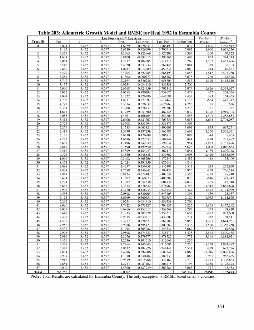
354
Table 203: Allometric Growth Model and RMSE for Real 1992 in Escambia County
Tract ID Log Pop = a + b * Log Area Pop Est-
PopAct
(PopEst-
PopAct)2 Pop a b Area Log Area Log_Pop AntilogPop
0 2,071 3.452 0.597 1.6929 0.228631 3.588493 3,877 1,806 3,261,542 1 3,192 3.452 0.597 2.6730 0.426999 3.706918 5,092 1,900 3,611,336
2 3,567 3.452 0.597 1.3365 0.125969 3.527203 3,367 -200 40,123
3 1,634 3.452 0.597 0.8100 -0.091515 3.397366 2,497 863 744,243
4 2,061 3.452 0.597 1.2717 0.104385 3.514318 3,268 1,207 1,457,496
5 5,512 3.452 0.597 3.4020 0.531734 3.769445 5,881 369 136,103
6 2,666 3.452 0.597 1.0287 0.012289 3.459336 2,880 214 45,637
7 6,470 3.452 0.597 2.4705 0.392785 3.686493 4,858 -1,612 2,597,280
8 3,284 3.452 0.597 1.1502 0.060773 3.488282 3,078 -206 42,398
9 5,747 3.452 0.597 2.2194 0.346236 3.658703 4,557 -1,190 1,415,510
10 3,157 3.452 0.597 0.9234 -0.034610 3.431338 2,700
11 6,900 3.452 0.597 2.6568 0.424359 3.705342 5,074 -1,826 3,334,627
12 5,022 3.452 0.597 3.0213 0.480194 3.738676 5,479 457 208,554
13 4,044 3.452 0.597 2.1222 0.326786 3.647091 4,437 393 154,465
14 4,780 3.452 0.597 1.8711 0.272097 3.614442 4,116 -664 441,317
15 4,728 3.452 0.597 2.3814 0.376832 3.676969 4,753 25 626
16 6,304 3.452 0.597 3.7908 0.578731 3.797502 6,273 -31 937
17 1,643 3.452 0.597 1.1259 0.051500 3.482745 3,039 1,396 1,949,103
18 2,055 3.452 0.597 1.4661 0.166164 3.551200 3,558 1,503 2,258,854
19 3,411 3.452 0.597 2.6406 0.421703 3.703756 5,055 1,644 2,704,087
20 2,725 3.452 0.597 1.3608 0.133794 3.531875 3,403
21 2,256 3.452 0.597 1.1583 0.063821 3.490101 3,091 835 697,251
22 2,413 3.452 0.597 1.5390 0.187239 3.563781 3,663 1,250 1,561,331
23 5,136 3.452 0.597 2.6730 0.426999 3.706918 5,092 -44 1,905
24 4,722 3.452 0.597 1.6686 0.222352 3.584744 3,844 -878 771,492
25 5,607 3.452 0.597 1.7496 0.242939 3.597034 3,954 -1,653 2,732,476
26 4,618 3.452 0.597 3.1590 0.499550 3.750231 5,626 1,008 1,016,884
27 2,512 3.452 0.597 1.5309 0.184947 3.562413 3,651 1,139 1,297,348
28 9,328 3.452 0.597 4.4550 0.648848 3.839362 6,908 -2,420 5,855,649
29 1,069 3.452 0.597 0.3402 -0.468266 3.172445 1,487 418 175,109
30 8,451 3.452 0.597 2.4624 0.391359 3.685641 4,849
31 2,998 3.452 0.597 1.4337 0.156458 3.545406 3,511 513 262,960
32 4,834 3.452 0.597 1.7658 0.246942 3.599424 3,976 -858 736,514
33 2,849 3.452 0.597 0.8424 -0.074482 3.407534 2,556 -293 85,940
34 3,694 3.452 0.597 1.1502 0.060773 3.488282 3,078 -616 379,342
35 4,224 3.452 0.597 1.7982 0.254838 3.604138 4,019 -205 41,948
36 6,665 3.452 0.597 2.3814 0.376832 3.676969 4,753 -1,912 3,655,698
37 4,902 3.452 0.597 1.3770 0.138934 3.534944 3,427 -1,475 2,174,939
38 4,555 3.452 0.597 2.0898 0.320105 3.643103 4,396 -159 25,137
39 7,175 3.452 0.597 3.6369 0.560731 3.786757 6,120 -1,055 1,112,870
40 2,262 3.452 0.597 0.9234 -0.034610 3.431338 2,700
41 8,090 3.452 0.597 3.7422 0.573127 3.794157 6,225 -1,865 3,477,292
42 2,039 3.452 0.597 0.6966 -0.157017 3.358261 2,282 243 58,910
43 6,649 3.452 0.597 3.1833 0.502878 3.752218 5,652 -997 993,600
44 2,472 3.452 0.597 0.9315 -0.030817 3.433602 2,714 242 58,541
45 4,585 3.452 0.597 3.3777 0.528621 3.767587 5,856 1,271 1,614,951
46 7,952 3.452 0.597 3.9366 0.595121 3.807287 6,416 -1,536 2,358,250
47 5,532 3.452 0.597 3.1995 0.505082 3.753534 5,669 137 18,868
48 7,998 3.452 0.597 2.9808 0.474333 3.735177 5,435 -2,563 6,570,435
49 7,916 3.452 0.597 2.3976 0.379777 3.678727 4,772 -3,144 9,882,921
50 4,460 3.452 0.597 1.2636 0.101610 3.512661 3,256
51 6,578 3.452 0.597 2.7864 0.445043 3.717691 5,220 -1,358 1,843,497
52 6,343 3.452 0.597 3.0537 0.484826 3.741441 5,514 -829 687,776
53 7,884 3.452 0.597 2.4786 0.394206 3.687341 4,868 -3,016 9,096,886
54 2,907 3.452 0.597 1.7010 0.230704 3.589730 3,888 981 962,435
55 3,913 3.452 0.597 0.9639 -0.015968 3.442467 2,770 -1,143 1,306,634
56 4,651 3.452 0.597 1.2231 0.087462 3.504215 3,193 -1,458 2,125,424
57 4,040 3.452 0.597 1.5390 0.187239 3.563781 3,663 -377 142,482
Total 265,252 119.0052 245,337 RMSE 1,324.93
Note: Total Results are calculated for Escambia County. The only exception is RMSE, based on all 3 counties.
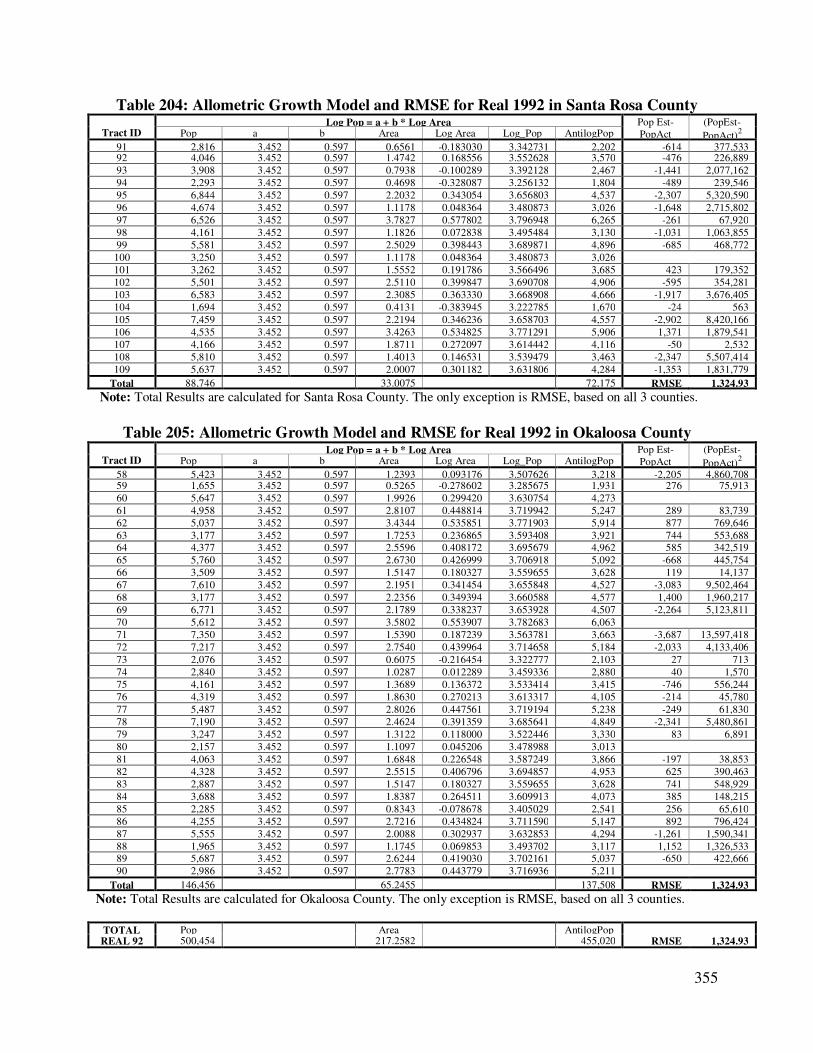
355
Table 204: Allometric Growth Model and RMSE for Real 1992 in Santa Rosa County
Tract ID Log Pop = a + b * Log Area Pop Est-
PopAct
(PopEst-
PopAct)2 Pop a b Area Log Area Log_Pop AntilogPop
91 2,816 3.452 0.597 0.6561 -0.183030 3.342731 2,202 -614 377,533 92 4,046 3.452 0.597 1.4742 0.168556 3.552628 3,570 -476 226,889
93 3,908 3.452 0.597 0.7938 -0.100289 3.392128 2,467 -1,441 2,077,162
94 2,293 3.452 0.597 0.4698 -0.328087 3.256132 1,804 -489 239,546
95 6,844 3.452 0.597 2.2032 0.343054 3.656803 4,537 -2,307 5,320,590
96 4,674 3.452 0.597 1.1178 0.048364 3.480873 3,026 -1,648 2,715,802
97 6,526 3.452 0.597 3.7827 0.577802 3.796948 6,265 -261 67,920
98 4,161 3.452 0.597 1.1826 0.072838 3.495484 3,130 -1,031 1,063,855
99 5,581 3.452 0.597 2.5029 0.398443 3.689871 4,896 -685 468,772
100 3,250 3.452 0.597 1.1178 0.048364 3.480873 3,026
101 3,262 3.452 0.597 1.5552 0.191786 3.566496 3,685 423 179,352
102 5,501 3.452 0.597 2.5110 0.399847 3.690708 4,906 -595 354,281
103 6,583 3.452 0.597 2.3085 0.363330 3.668908 4,666 -1,917 3,676,405
104 1,694 3.452 0.597 0.4131 -0.383945 3.222785 1,670 -24 563
105 7,459 3.452 0.597 2.2194 0.346236 3.658703 4,557 -2,902 8,420,166
106 4,535 3.452 0.597 3.4263 0.534825 3.771291 5,906 1,371 1,879,541
107 4,166 3.452 0.597 1.8711 0.272097 3.614442 4,116 -50 2,532
108 5,810 3.452 0.597 1.4013 0.146531 3.539479 3,463 -2,347 5,507,414
109 5,637 3.452 0.597 2.0007 0.301182 3.631806 4,284 -1,353 1,831,779
Total 88,746 33.0075 72,175 RMSE 1,324.93
Note: Total Results are calculated for Santa Rosa County. The only exception is RMSE, based on all 3 counties.
Table 205: Allometric Growth Model and RMSE for Real 1992 in Okaloosa County
Tract ID Log Pop = a + b * Log Area Pop Est-
PopAct
(PopEst-
PopAct)2 Pop a b Area Log Area Log_Pop AntilogPop
58 5,423 3.452 0.597 1.2393 0.093176 3.507626 3,218 -2,205 4,860,708 59 1,655 3.452 0.597 0.5265 -0.278602 3.285675 1,931 276 75,913
60 5,647 3.452 0.597 1.9926 0.299420 3.630754 4,273
61 4,958 3.452 0.597 2.8107 0.448814 3.719942 5,247 289 83,739
62 5,037 3.452 0.597 3.4344 0.535851 3.771903 5,914 877 769,646
63 3,177 3.452 0.597 1.7253 0.236865 3.593408 3,921 744 553,688
64 4,377 3.452 0.597 2.5596 0.408172 3.695679 4,962 585 342,519
65 5,760 3.452 0.597 2.6730 0.426999 3.706918 5,092 -668 445,754
66 3,509 3.452 0.597 1.5147 0.180327 3.559655 3,628 119 14,137
67 7,610 3.452 0.597 2.1951 0.341454 3.655848 4,527 -3,083 9,502,464
68 3,177 3.452 0.597 2.2356 0.349394 3.660588 4,577 1,400 1,960,217
69 6,771 3.452 0.597 2.1789 0.338237 3.653928 4,507 -2,264 5,123,811
70 5,612 3.452 0.597 3.5802 0.553907 3.782683 6,063
71 7,350 3.452 0.597 1.5390 0.187239 3.563781 3,663 -3,687 13,597,418
72 7,217 3.452 0.597 2.7540 0.439964 3.714658 5,184 -2,033 4,133,406
73 2,076 3.452 0.597 0.6075 -0.216454 3.322777 2,103 27 713
74 2,840 3.452 0.597 1.0287 0.012289 3.459336 2,880 40 1,570
75 4,161 3.452 0.597 1.3689 0.136372 3.533414 3,415 -746 556,244
76 4,319 3.452 0.597 1.8630 0.270213 3.613317 4,105 -214 45,780
77 5,487 3.452 0.597 2.8026 0.447561 3.719194 5,238 -249 61,830
78 7,190 3.452 0.597 2.4624 0.391359 3.685641 4,849 -2,341 5,480,861
79 3,247 3.452 0.597 1.3122 0.118000 3.522446 3,330 83 6,891
80 2,157 3.452 0.597 1.1097 0.045206 3.478988 3,013
81 4,063 3.452 0.597 1.6848 0.226548 3.587249 3,866 -197 38,853
82 4,328 3.452 0.597 2.5515 0.406796 3.694857 4,953 625 390,463
83 2,887 3.452 0.597 1.5147 0.180327 3.559655 3,628 741 548,929
84 3,688 3.452 0.597 1.8387 0.264511 3.609913 4,073 385 148,215
85 2,285 3.452 0.597 0.8343 -0.078678 3.405029 2,541 256 65,610
86 4,255 3.452 0.597 2.7216 0.434824 3.711590 5,147 892 796,424
87 5,555 3.452 0.597 2.0088 0.302937 3.632853 4,294 -1,261 1,590,341
88 1,965 3.452 0.597 1.1745 0.069853 3.493702 3,117 1,152 1,326,533
89 5,687 3.452 0.597 2.6244 0.419030 3.702161 5,037 -650 422,666
90 2,986 3.452 0.597 2.7783 0.443779 3.716936 5,211
Total 146,456 65.2455 137,508 RMSE 1,324.93
Note: Total Results are calculated for Okaloosa County. The only exception is RMSE, based on all 3 counties.
TOTAL Pop
Area
AntilogPop REAL 92 500,454 217.2582 455,020 RMSE 1,324.93
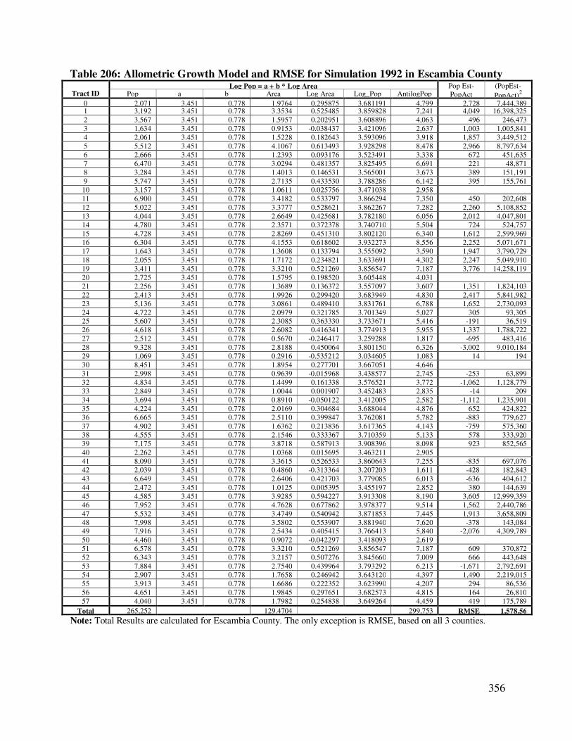
356
Table 206: Allometric Growth Model and RMSE for Simulation 1992 in Escambia County
Tract ID Log Pop = a + b * Log Area Pop Est-
PopAct
(PopEst-
PopAct)2 Pop a b Area Log Area Log_Pop AntilogPop
0 2,071 3.451 0.778 1.9764 0.295875 3.681191 4,799 2,728 7,444,389 1 3,192 3.451 0.778 3.3534 0.525485 3.859828 7,241 4,049 16,398,325
2 3,567 3.451 0.778 1.5957 0.202951 3.608896 4,063 496 246,473
3 1,634 3.451 0.778 0.9153 -0.038437 3.421096 2,637 1,003 1,005,841
4 2,061 3.451 0.778 1.5228 0.182643 3.593096 3,918 1,857 3,449,512
5 5,512 3.451 0.778 4.1067 0.613493 3.928298 8,478 2,966 8,797,634
6 2,666 3.451 0.778 1.2393 0.093176 3.523491 3,338 672 451,635
7 6,470 3.451 0.778 3.0294 0.481357 3.825495 6,691 221 48,871
8 3,284 3.451 0.778 1.4013 0.146531 3.565001 3,673 389 151,191
9 5,747 3.451 0.778 2.7135 0.433530 3.788286 6,142 395 155,761
10 3,157 3.451 0.778 1.0611 0.025756 3.471038 2,958
11 6,900 3.451 0.778 3.4182 0.533797 3.866294 7,350 450 202,608
12 5,022 3.451 0.778 3.3777 0.528621 3.862267 7,282 2,260 5,108,852
13 4,044 3.451 0.778 2.6649 0.425681 3.782180 6,056 2,012 4,047,801
14 4,780 3.451 0.778 2.3571 0.372378 3.740710 5,504 724 524,757
15 4,728 3.451 0.778 2.8269 0.451310 3.802120 6,340 1,612 2,599,969
16 6,304 3.451 0.778 4.1553 0.618602 3.932273 8,556 2,252 5,071,671
17 1,643 3.451 0.778 1.3608 0.133794 3.555092 3,590 1,947 3,790,729
18 2,055 3.451 0.778 1.7172 0.234821 3.633691 4,302 2,247 5,049,910
19 3,411 3.451 0.778 3.3210 0.521269 3.856547 7,187 3,776 14,258,119
20 2,725 3.451 0.778 1.5795 0.198520 3.605448 4,031
21 2,256 3.451 0.778 1.3689 0.136372 3.557097 3,607 1,351 1,824,103
22 2,413 3.451 0.778 1.9926 0.299420 3.683949 4,830 2,417 5,841,982
23 5,136 3.451 0.778 3.0861 0.489410 3.831761 6,788 1,652 2,730,093
24 4,722 3.451 0.778 2.0979 0.321785 3.701349 5,027 305 93,305
25 5,607 3.451 0.778 2.3085 0.363330 3.733671 5,416 -191 36,519
26 4,618 3.451 0.778 2.6082 0.416341 3.774913 5,955 1,337 1,788,722
27 2,512 3.451 0.778 0.5670 -0.246417 3.259288 1,817 -695 483,416
28 9,328 3.451 0.778 2.8188 0.450064 3.801150 6,326 -3,002 9,010,184
29 1,069 3.451 0.778 0.2916 -0.535212 3.034605 1,083 14 194
30 8,451 3.451 0.778 1.8954 0.277701 3.667051 4,646
31 2,998 3.451 0.778 0.9639 -0.015968 3.438577 2,745 -253 63,899
32 4,834 3.451 0.778 1.4499 0.161338 3.576521 3,772 -1,062 1,128,779
33 2,849 3.451 0.778 1.0044 0.001907 3.452483 2,835 -14 209
34 3,694 3.451 0.778 0.8910 -0.050122 3.412005 2,582 -1,112 1,235,901
35 4,224 3.451 0.778 2.0169 0.304684 3.688044 4,876 652 424,822
36 6,665 3.451 0.778 2.5110 0.399847 3.762081 5,782 -883 779,627
37 4,902 3.451 0.778 1.6362 0.213836 3.617365 4,143 -759 575,360
38 4,555 3.451 0.778 2.1546 0.333367 3.710359 5,133 578 333,920
39 7,175 3.451 0.778 3.8718 0.587913 3.908396 8,098 923 852,565
40 2,262 3.451 0.778 1.0368 0.015695 3.463211 2,905
41 8,090 3.451 0.778 3.3615 0.526533 3.860643 7,255 -835 697,076
42 2,039 3.451 0.778 0.4860 -0.313364 3.207203 1,611 -428 182,843
43 6,649 3.451 0.778 2.6406 0.421703 3.779085 6,013 -636 404,612
44 2,472 3.451 0.778 1.0125 0.005395 3.455197 2,852 380 144,639
45 4,585 3.451 0.778 3.9285 0.594227 3.913308 8,190 3,605 12,999,359
46 7,952 3.451 0.778 4.7628 0.677862 3.978377 9,514 1,562 2,440,786
47 5,532 3.451 0.778 3.4749 0.540942 3.871853 7,445 1,913 3,658,809
48 7,998 3.451 0.778 3.5802 0.553907 3.881940 7,620 -378 143,084
49 7,916 3.451 0.778 2.5434 0.405415 3.766413 5,840 -2,076 4,309,789
50 4,460 3.451 0.778 0.9072 -0.042297 3.418093 2,619
51 6,578 3.451 0.778 3.3210 0.521269 3.856547 7,187 609 370,872
52 6,343 3.451 0.778 3.2157 0.507276 3.845660 7,009 666 443,648
53 7,884 3.451 0.778 2.7540 0.439964 3.793292 6,213 -1,671 2,792,691
54 2,907 3.451 0.778 1.7658 0.246942 3.643120 4,397 1,490 2,219,015
55 3,913 3.451 0.778 1.6686 0.222352 3.623990 4,207 294 86,536
56 4,651 3.451 0.778 1.9845 0.297651 3.682573 4,815 164 26,810
57 4,040 3.451 0.778 1.7982 0.254838 3.649264 4,459 419 175,789
Total 265,252 129.4704 299,753 RMSE 1,578.56
Note: Total Results are calculated for Escambia County. The only exception is RMSE, based on all 3 counties.

357
Table 207: Allometric Growth Model and RMSE for Simulation 1992 in Sta. Rosa County
Tract ID Log Pop = a + b * Log Area Pop Est-
PopAct
(PopEst-
PopAct)2 Pop a b Area Log Area Log_Pop AntilogPop
91 2,816 3.451 0.778 1.5228 0.182643 3.593096 3,918 1,102 1,215,035 92 4,046 3.451 0.778 1.8711 0.272097 3.662691 4,599 553 306,138
93 3,908 3.451 0.778 0.8586 -0.066209 3.399489 2,509 -1,399 1,957,385
94 2,293 3.451 0.778 1.0611 0.025756 3.471038 2,958 665 442,590
95 6,844 3.451 0.778 2.7459 0.438685 3.792297 6,199 -645 416,484
96 4,674 3.451 0.778 1.4499 0.161338 3.576521 3,772 -902 814,398
97 6,526 3.451 0.778 4.3902 0.642484 3.950853 8,930 2,404 5,779,348
98 4,161 3.451 0.778 1.3689 0.136372 3.557097 3,607 -554 307,367
99 5,581 3.451 0.778 1.9602 0.292300 3.678410 4,769 -812 659,658
100 3,250 3.451 0.778 1.5147 0.180327 3.591294 3,902
101 3,262 3.451 0.778 1.8387 0.264511 3.656789 4,537 1,275 1,626,176
102 5,501 3.451 0.778 2.9646 0.471966 3.818190 6,579 1,078 1,163,056
103 6,583 3.451 0.778 2.7783 0.443779 3.796260 6,255 -328 107,274
104 1,694 3.451 0.778 0.5346 -0.271971 3.239407 1,735 41 1,716
105 7,459 3.451 0.778 1.7739 0.248929 3.644667 4,412 -3,047 9,282,267
106 4,535 3.451 0.778 1.1745 0.069853 3.505346 3,201 -1,334 1,778,377
107 4,166 3.451 0.778 1.1097 0.045206 3.486170 3,063 -1,103 1,216,252
108 5,810 3.451 0.778 0.8100 -0.091515 3.379801 2,398 -3,412 11,643,546
109 5,637 3.451 0.778 1.8630 0.270213 3.661226 4,584 -1,053 1,109,232
Total 88,746 33.5907 81,929 RMSE 1,578.56
Note: Total Results are calculated for Santa Rosa County. The only exception is RMSE, based on all 3 counties.
Table 208: Allometric Growth Model and RMSE for Simulation 1992 in Okaloosa County
Tract ID Log Pop = a + b * Log Area Pop Est-
PopAct
(PopEst-
PopAct)2 Pop a b Area Log Area Log_Pop AntilogPop
58 5,423 3.451 0.778 1.5147 0.180327 3.591294 3,902 -1,521 2,313,254 59 1,655 3.451 0.778 0.5832 -0.234182 3.268806 1,857 202 40,794
60 5,647 3.451 0.778 1.5552 0.191786 3.600210 3,983
61 4,958 3.451 0.778 2.6973 0.430929 3.786263 6,113 1,155 1,334,303
62 5,037 3.451 0.778 3.2400 0.510545 3.848204 7,050 2,013 4,053,143
63 3,177 3.451 0.778 1.3527 0.131201 3.553075 3,573 396 157,088
64 4,377 3.451 0.778 2.3166 0.364851 3.734854 5,431 1,054 1,110,239
65 5,760 3.451 0.778 1.6200 0.209515 3.614003 4,112 -1,648 2,717,478
66 3,509 3.451 0.778 1.0935 0.038819 3.481201 3,028 -481 231,058
67 7,610 3.451 0.778 1.0854 0.035590 3.478689 3,011 -4,599 21,152,196
68 3,177 3.451 0.778 2.0007 0.301182 3.685320 4,845 1,668 2,783,184
69 6,771 3.451 0.778 2.1141 0.325126 3.703948 5,058 -1,713 2,935,613
70 5,612 3.451 0.778 2.3814 0.376832 3.744176 5,548
71 7,350 3.451 0.778 1.3203 0.120673 3.544883 3,507 -3,843 14,771,905
72 7,217 3.451 0.778 2.7702 0.442511 3.795274 6,241 -976 952,030
73 2,076 3.451 0.778 0.6399 -0.193888 3.300155 1,996 -80 6,404
74 2,840 3.451 0.778 1.0125 0.005395 3.455197 2,852 12 152
75 4,161 3.451 0.778 0.7695 -0.113791 3.362470 2,304 -1,857 3,448,689
76 4,319 3.451 0.778 1.4094 0.149034 3.566949 3,689 -630 396,472
77 5,487 3.451 0.778 2.0493 0.311606 3.693429 4,937 -550 302,926
78 7,190 3.451 0.778 3.0537 0.484826 3.828195 6,733 -457 209,043
79 3,247 3.451 0.778 1.5228 0.182643 3.593096 3,918 671 450,625
80 2,157 3.451 0.778 1.3284 0.123329 3.546950 3,523
81 4,063 3.451 0.778 2.0655 0.315025 3.696090 4,967 904 817,122
82 4,328 3.451 0.778 2.7945 0.446304 3.798225 6,284 1,956 3,825,281
83 2,887 3.451 0.778 1.6443 0.215981 3.619033 4,159 1,272 1,619,065
84 3,688 3.451 0.778 2.0250 0.306425 3.689399 4,891 1,203 1,447,236
85 2,285 3.451 0.778 0.9153 -0.038437 3.421096 2,637 352 123,845
86 4,255 3.451 0.778 2.3328 0.367878 3.737209 5,460 1,205 1,452,512
87 5,555 3.451 0.778 2.0817 0.318418 3.698729 4,997 -558 311,108
88 1,965 3.451 0.778 0.8262 -0.082915 3.386492 2,435 470 220,865
89 5,687 3.451 0.778 1.5309 0.184947 3.594889 3,934 -1,753 3,071,286
90 2,986 3.451 0.778 1.4823 0.170936 3.583988 3,837
Total 146,456 57.1293 140,814 RMSE 1,578.56
Note: Total Results are calculated for Okaloosa County. The only exception is RMSE, based on all 3 counties.
TOTAL Pop
Area
AntilogPop SIM 92 500,454 220.1904 522,495 RMSE 1,578.56
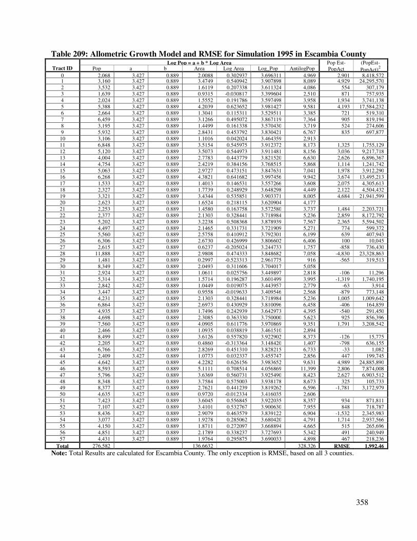
358
Table 209: Allometric Growth Model and RMSE for Simulation 1995 in Escambia County
Tract ID Log Pop = a + b * Log Area Pop Est-
PopAct
(PopEst-
PopAct)2 Pop a b Area Log Area Log_Pop AntilogPop
0 2,068 3.427 0.889 2.0088 0.302937 3.696311 4,969 2,901 8,418,572 1 3,160 3.427 0.889 3.4749 0.540942 3.907898 8,089 4,929 24,295,570
2 3,532 3.427 0.889 1.6119 0.207338 3.611324 4,086 554 307,179
3 1,639 3.427 0.889 0.9315 -0.030817 3.399604 2,510 871 757,935
4 2,024 3.427 0.889 1.5552 0.191786 3.597498 3,958 1,934 3,741,138
5 5,388 3.427 0.889 4.2039 0.623652 3.981427 9,581 4,193 17,584,232
6 2,664 3.427 0.889 1.3041 0.115311 3.529511 3,385 721 519,310
7 6,459 3.427 0.889 3.1266 0.495072 3.867119 7,364 905 819,194
8 3,195 3.427 0.889 1.4499 0.161338 3.570430 3,719 524 274,606
9 5,932 3.427 0.889 2.8431 0.453792 3.830421 6,767 835 697,877
10 3,106 3.427 0.889 1.1016 0.042024 3.464359 2,913
11 6,848 3.427 0.889 3.5154 0.545975 3.912372 8,173 1,325 1,755,129
12 5,120 3.427 0.889 3.5073 0.544973 3.911481 8,156 3,036 9,217,718
13 4,004 3.427 0.889 2.7783 0.443779 3.821520 6,630 2,626 6,896,367
14 4,754 3.427 0.889 2.4219 0.384156 3.768515 5,868 1,114 1,241,742
15 5,063 3.427 0.889 2.9727 0.473151 3.847631 7,041 1,978 3,912,290
16 6,268 3.427 0.889 4.3821 0.641682 3.997456 9,942 3,674 13,495,213
17 1,533 3.427 0.889 1.4013 0.146531 3.557266 3,608 2,075 4,305,613
18 2,327 3.427 0.889 1.7739 0.248929 3.648298 4,449 2,122 4,504,432
19 3,321 3.427 0.889 3.4344 0.535851 3.903371 8,005 4,684 21,941,599
20 2,623 3.427 0.889 1.6524 0.218115 3.620904 4,177
21 2,253 3.427 0.889 1.4580 0.163758 3.572580 3,737 1,484 2,203,721
22 2,377 3.427 0.889 2.1303 0.328441 3.718984 5,236 2,859 8,172,792
23 5,202 3.427 0.889 3.2238 0.508368 3.878939 7,567 2,365 5,594,502
24 4,497 3.427 0.889 2.1465 0.331731 3.721909 5,271 774 599,372
25 5,560 3.427 0.889 2.5758 0.410912 3.792301 6,199 639 407,943
26 6,306 3.427 0.889 2.6730 0.426999 3.806602 6,406 100 10,045
27 2,615 3.427 0.889 0.6237 -0.205024 3.244733 1,757 -858 736,430
28 11,888 3.427 0.889 2.9808 0.474333 3.848682 7,058 -4,830 23,328,863
29 1,481 3.427 0.889 0.2997 -0.523313 2.961775 916 -565 319,513
30 8,349 3.427 0.889 2.0493 0.311606 3.704017 5,058
31 2,924 3.427 0.889 1.0611 0.025756 3.449897 2,818 -106 11,296
32 5,314 3.427 0.889 1.5714 0.196287 3.601499 3,995 -1,319 1,740,195
33 2,842 3.427 0.889 1.0449 0.019075 3.443957 2,779 -63 3,914
34 3,447 3.427 0.889 0.9558 -0.019633 3.409546 2,568 -879 773,148
35 4,231 3.427 0.889 2.1303 0.328441 3.718984 5,236 1,005 1,009,642
36 6,864 3.427 0.889 2.6973 0.430929 3.810096 6,458 -406 164,859
37 4,935 3.427 0.889 1.7496 0.242939 3.642973 4,395 -540 291,450
38 4,698 3.427 0.889 2.3085 0.363330 3.750000 5,623 925 856,396
39 7,560 3.427 0.889 4.0905 0.611776 3.970869 9,351 1,791 3,208,542
40 2,466 3.427 0.889 1.0935 0.038819 3.461510 2,894
41 8,499 3.427 0.889 3.6126 0.557820 3.922902 8,373 -126 15,775
42 2,205 3.427 0.889 0.4860 -0.313364 3.148420 1,407 -798 636,155
43 6,766 3.427 0.889 2.8269 0.451310 3.828215 6,733 -33 1,082
44 2,409 3.427 0.889 1.0773 0.032337 3.455747 2,856 447 199,745
45 4,642 3.427 0.889 4.2282 0.626156 3.983652 9,631 4,989 24,885,890
46 8,593 3.427 0.889 5.1111 0.708514 4.056869 11,399 2,806 7,874,008
47 5,796 3.427 0.889 3.6369 0.560731 3.925490 8,423 2,627 6,903,512
48 8,348 3.427 0.889 3.7584 0.575003 3.938178 8,673 325 105,733
49 8,377 3.427 0.889 2.7621 0.441239 3.819262 6,596 -1,781 3,172,979
50 4,635 3.427 0.889 0.9720 -0.012334 3.416035 2,606
51 7,423 3.427 0.889 3.6045 0.556845 3.922035 8,357 934 871,811
52 7,107 3.427 0.889 3.4101 0.532767 3.900630 7,955 848 718,787
53 8,436 3.427 0.889 2.9079 0.463579 3.839122 6,904 -1,532 2,345,983
54 3,077 3.427 0.889 1.9278 0.285062 3.680420 4,791 1,714 2,937,566
55 4,150 3.427 0.889 1.8711 0.272097 3.668894 4,665 515 265,696
56 4,851 3.427 0.889 2.1789 0.338237 3.727693 5,342 491 240,949
57 4,431 3.427 0.889 1.9764 0.295875 3.690033 4,898 467 218,236
Total 276,582 136.6632 328,326 RMSE 1,992.46
Note: Total Results are calculated for Escambia County. The only exception is RMSE, based on all 3 counties.

359
Table 210: Allometric Growth Model and RMSE for Simulation 1995 in Sta. Rosa County
Tract ID Log Pop = a + b * Log Area Pop Est-
PopAct
(PopEst-
PopAct)2 Pop a b Area Log Area Log_Pop AntilogPop
91 3,113 3.427 0.889 1.7091 0.232767 3.633930 4,305 1,192 1,419,851 92 4,108 3.427 0.889 2.0331 0.308159 3.700953 5,023 915 837,012
93 4,791 3.427 0.889 0.9720 -0.012334 3.416035 2,606 -2,185 4,772,628
94 2,285 3.427 0.889 1.1907 0.075802 3.494388 3,122 837 700,032
95 7,334 3.427 0.889 2.9889 0.475511 3.849730 7,075 -259 67,054
96 5,186 3.427 0.889 1.5876 0.200741 3.605459 4,031 -1,155 1,333,038
97 6,408 3.427 0.889 4.6413 0.666640 4.019643 10,463 4,055 16,440,371
98 4,457 3.427 0.889 1.4985 0.175657 3.583159 3,830 -627 393,571
99 6,472 3.427 0.889 2.0736 0.316725 3.708569 5,112 -1,360 1,850,315
100 3,400 3.427 0.889 1.6281 0.211681 3.615184 4,123
101 3,241 3.427 0.889 1.9278 0.285062 3.680420 4,791 1,550 2,402,292
102 5,982 3.427 0.889 3.1914 0.503981 3.875039 7,500 1,518 2,303,174
103 7,787 3.427 0.889 3.0780 0.488269 3.861071 7,262 -525 275,370
104 2,288 3.427 0.889 0.5346 -0.271971 3.185218 1,532 -756 571,755
105 7,971 3.427 0.889 1.9035 0.279553 3.675523 4,737 -3,234 10,457,407
106 6,077 3.427 0.889 1.2069 0.081671 3.499606 3,159 -2,918 8,512,340
107 5,235 3.427 0.889 1.1745 0.069853 3.489099 3,084 -2,151 4,627,260
108 6,864 3.427 0.889 0.9315 -0.030817 3.399604 2,510 -4,354 18,960,847
109 5,690 3.427 0.889 1.9440 0.288696 3.683651 4,827 -863 745,274
Total 98,689 36.2151 89,090 RMSE 1,992.46
Note: Total Results are calculated for Santa Rosa County. The only exception is RMSE, based on all 3 counties.
Table 211: Allometric Growth Model and RMSE for Simulation 1995 in Okaloosa County
Tract ID Log Pop = a + b * Log Area Pop Est-
PopAct
(PopEst-
PopAct)2 Pop a b Area Log Area Log_Pop AntilogPop
58 5,907 3.427 0.889 1.7010 0.230704 3.632096 4,286 -1,621 2,626,234 59 1,715 3.427 0.889 0.6561 -0.183030 3.264286 1,838 123 15,067
60 6,606 3.427 0.889 1.8387 0.264511 3.662150 4,594
61 5,185 3.427 0.889 2.9241 0.465992 3.841267 6,939 1,754 3,074,846
62 5,216 3.427 0.889 3.4587 0.538913 3.906094 8,056 2,840 8,062,872
63 3,881 3.427 0.889 1.4580 0.163758 3.572580 3,737 -144 20,594
64 5,446 3.427 0.889 2.4786 0.394206 3.777450 5,990 544 296,277
65 5,635 3.427 0.889 1.6767 0.224455 3.626541 4,232 -1,403 1,968,541
66 3,891 3.427 0.889 1.1502 0.060773 3.481028 3,027 -864 746,314
67 8,355 3.427 0.889 1.1988 0.078747 3.497006 3,141 -5,214 27,190,479
68 3,238 3.427 0.889 2.0817 0.318418 3.710074 5,129 1,891 3,577,714
69 6,979 3.427 0.889 2.2437 0.350965 3.739008 5,483 -1,496 2,238,415
70 6,279 3.427 0.889 2.4219 0.384156 3.768515 5,868
71 7,370 3.427 0.889 1.4013 0.146531 3.557266 3,608 -3,762 14,152,667
72 7,502 3.427 0.889 2.8836 0.459935 3.835882 6,853 -649 421,170
73 1,994 3.427 0.889 0.7047 -0.151996 3.291876 1,958 -36 1,276
74 2,778 3.427 0.889 1.0773 0.032337 3.455747 2,856 78 6,073
75 4,573 3.427 0.889 0.8181 -0.087194 3.349485 2,236 -2,337 5,461,254
76 4,620 3.427 0.889 1.4661 0.166164 3.574719 3,756 -864 746,588
77 5,803 3.427 0.889 2.1384 0.330089 3.720449 5,254 -549 301,946
78 7,149 3.427 0.889 3.1590 0.499550 3.871100 7,432 283 80,030
79 3,247 3.427 0.889 1.5552 0.191786 3.597498 3,958 711 505,809
80 2,233 3.427 0.889 1.4013 0.146531 3.557266 3,608
81 4,071 3.427 0.889 2.1789 0.338237 3.727693 5,342 1,271 1,615,099
82 4,253 3.427 0.889 2.8593 0.456260 3.832615 6,802 2,549 6,495,666
83 2,894 3.427 0.889 1.7010 0.230704 3.632096 4,286 1,392 1,938,872
84 3,705 3.427 0.889 2.0979 0.321785 3.713067 5,165 1,460 2,131,473
85 2,199 3.427 0.889 0.9396 -0.027057 3.402946 2,529 330 108,890
86 4,237 3.427 0.889 2.4543 0.389928 3.773646 5,938 1,701 2,893,656
87 6,220 3.427 0.889 2.1951 0.341454 3.730553 5,377 -843 710,381
88 1,919 3.427 0.889 0.8748 -0.058091 3.375357 2,373 454 206,410
89 6,863 3.427 0.889 1.6524 0.218115 3.620904 4,177 -2,686 7,212,533
90 3,075 3.427 0.889 1.5876 0.200741 3.605459 4,031
Total 155,038 60.4341 149,860 RMSE 1,992.46
Note: Total Results are calculated for Okaloosa County. The only exception is RMSE, based on all 3 counties.
TOTAL Pop
Area
AntilogPop SIM 95 530,309 233.3124 567,276 RMSE 1,992.46
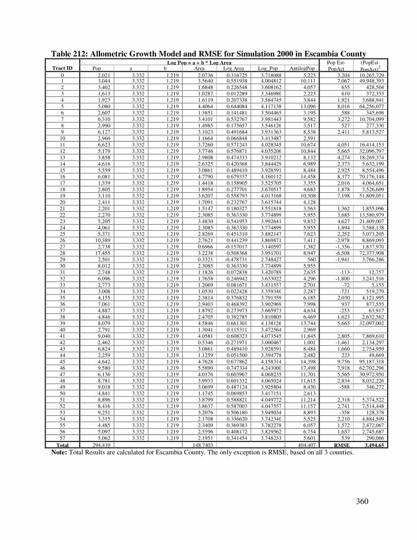
360
Table 212: Allometric Growth Model and RMSE for Simulation 2000 in Escambia County
Tract ID Log Pop = a + b * Log Area Pop Est-
PopAct
(PopEst-
PopAct)2 Pop a b Area Log Area Log_Pop AntilogPop
0 2,021 3.332 1.219 2.0736 0.316725 3.718088 5,225 3,204 10,265,729 1 3,044 3.332 1.219 3.5640 0.551938 4.004812 10,111 7,067 49,948,393
2 3,402 3.332 1.219 1.6848 0.226548 3.608162 4,057 655 428,504
3 1,613 3.332 1.219 1.0287 0.012289 3.346980 2,223 610 372,353
4 1,923 3.332 1.219 1.6119 0.207338 3.584745 3,844 1,921 3,688,941
5 5,080 3.332 1.219 4.4064 0.644084 4.117138 13,096 8,016 64,256,077
6 2,607 3.332 1.219 1.3851 0.141481 3.504465 3,195 588 345,698
7 6,310 3.332 1.219 3.4101 0.532767 3.981443 9,582 3,272 10,704,099
8 2,990 3.332 1.219 1.4985 0.175657 3.546126 3,517 527 277,330
9 6,127 3.332 1.219 3.1023 0.491684 3.931363 8,538 2,411 5,813,527
10 2,960 3.332 1.219 1.1664 0.066848 3.413487 2,591
11 6,623 3.332 1.219 3.7260 0.571243 4.028345 10,674 4,051 16,414,153
12 5,179 3.332 1.219 3.7746 0.576871 4.035206 10,844 5,665 32,096,797
13 3,858 3.332 1.219 2.9808 0.474333 3.910212 8,132 4,274 18,269,374
14 4,616 3.332 1.219 2.6325 0.420368 3.844429 6,989 2,373 5,632,199
15 5,559 3.332 1.219 3.0861 0.489410 3.928591 8,484 2,925 8,554,496
16 6,081 3.332 1.219 4.7790 0.679337 4.160112 14,458 8,377 70,176,148
17 1,339 3.332 1.219 1.4418 0.158905 3.525705 3,355 2,016 4,064,651
18 2,805 3.332 1.219 1.8954 0.277701 3.670517 4,683 1,878 3,526,609
19 3,110 3.332 1.219 3.6207 0.558793 4.013168 10,308 7,198 51,809,051
20 2,411 3.332 1.219 1.7091 0.232767 3.615744 4,128
21 2,201 3.332 1.219 1.5147 0.180327 3.551818 3,563 1,362 1,855,096
22 2,270 3.332 1.219 2.3085 0.363330 3.774899 5,955 3,685 13,580,979
23 5,205 3.332 1.219 3.4830 0.541953 3.992641 9,832 4,627 21,409,007
24 4,061 3.332 1.219 2.3085 0.363330 3.774899 5,955 1,894 3,588,138
25 5,371 3.332 1.219 2.8269 0.451310 3.882147 7,623 2,252 5,073,205
26 10,389 3.332 1.219 2.7621 0.441239 3.869871 7,411 -2,978 8,869,093
27 2,738 3.332 1.219 0.6966 -0.157017 3.140597 1,382 -1,356 1,837,970
28 17,455 3.332 1.219 3.2238 0.508368 3.951701 8,947 -8,508 72,377,908
29 2,501 3.332 1.219 0.3321 -0.478731 2.748427 560 -1,941 3,766,286
30 8,012 3.332 1.219 2.3085 0.363330 3.774899 5,955
31 2,748 3.332 1.219 1.1826 0.072838 3.420789 2,635 -113 12,757
32 6,096 3.332 1.219 1.7658 0.246942 3.633022 4,296 -1,800 3,241,516
33 2,773 3.332 1.219 1.2069 0.081671 3.431557 2,701 -72 5,155
34 3,008 3.332 1.219 1.0530 0.022428 3.359340 2,287 -721 519,279
35 4,155 3.332 1.219 2.3814 0.376832 3.791359 6,185 2,030 4,121,995
36 7,061 3.332 1.219 2.9403 0.468392 3.902969 7,998 937 877,555
37 4,887 3.332 1.219 1.8792 0.273973 3.665973 4,634 -253 63,917
38 4,846 3.332 1.219 2.4705 0.392785 3.810805 6,469 1,623 2,632,562
39 8,079 3.332 1.219 4.5846 0.661301 4.138126 13,744 5,665 32,097,002
40 2,791 3.332 1.219 1.3041 0.115311 3.472564 2,969
41 9,040 3.332 1.219 4.0581 0.608323 4.073545 11,845 2,805 7,869,610
42 2,462 3.332 1.219 0.5346 -0.271971 3.000467 1,001 -1,461 2,134,297
43 6,824 3.332 1.219 3.0861 0.489410 3.928591 8,484 1,660 2,754,959
44 2,259 3.332 1.219 1.1259 0.051500 3.394778 2,482 223 49,669
45 4,642 3.332 1.219 4.7628 0.677862 4.158314 14,398 9,756 95,187,318
46 9,580 3.332 1.219 5.5890 0.747334 4.243000 17,498 7,918 62,702,296
47 6,136 3.332 1.219 4.0176 0.603967 4.068235 11,701 5,565 30,972,950
48 8,781 3.332 1.219 3.9933 0.601332 4.065024 11,615 2,834 8,032,226
49 9,018 3.332 1.219 3.0699 0.487124 3.925804 8,430 -588 346,272
50 4,841 3.332 1.219 1.1745 0.069853 3.417151 2,613
51 8,896 3.332 1.219 3.8799 0.588821 4.049772 11,214 2,318 5,374,522
52 8,416 3.332 1.219 3.8637 0.587003 4.047557 11,157 2,741 7,514,448
53 9,251 3.332 1.219 3.2076 0.506180 3.949034 8,893 -358 128,378
54 3,315 3.332 1.219 2.1708 0.336620 3.742340 5,525 2,210 4,884,509
55 4,485 3.332 1.219 2.3409 0.369383 3.782278 6,057 1,572 2,472,067
56 5,097 3.332 1.219 2.5596 0.408172 3.829562 6,754 1,657 2,745,687
57 5,062 3.332 1.219 2.1951 0.341454 3.748233 5,601 539 290,066
Total 294,410 148.7403 404,407 RMSE 3,494.65
Note: Total Results are calculated for Escambia County. The only exception is RMSE, based on all 3 counties.
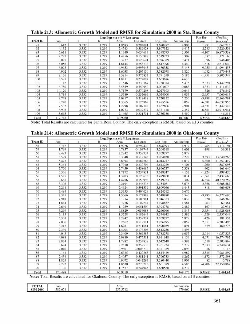
361
Table 213: Allometric Growth Model and RMSE for Simulation 2000 in Sta. Rosa County
Tract ID Log Pop = a + b * Log Area Pop Est-
PopAct
(PopEst-
PopAct)2 Pop a b Area Log Area Log_Pop AntilogPop
91 3,612 3.332 1.219 1.9683 0.294091 3.690497 4,903 1,291 1,667,713 92 4,132 3.332 1.219 2.4543 0.389928 3.807322 6,417 2,285 5,220,534
93 6,611 3.332 1.219 1.1340 0.054613 3.398573 2,504 -4,107 16,870,338
94 2,227 3.332 1.219 1.4256 0.153998 3.519723 3,309 1,082 1,171,160
95 8,075 3.332 1.219 3.3777 0.528621 3.976389 9,471 1,396 1,948,405
96 6,056 3.332 1.219 1.8144 0.258733 3.647396 4,440 -1,616 2,611,040
97 6,093 3.332 1.219 4.9653 0.695945 4.180358 15,148 9,055 81,994,453
98 4,902 3.332 1.219 1.6038 0.205150 3.582078 3,820 -1,082 1,170,443
99 8,136 3.332 1.219 2.3814 0.376832 3.791359 6,185 -1,951 3,805,349
100 3,595 3.332 1.219 1.8711 0.272097 3.663686 4,610
101 3,142 3.332 1.219 2.1546 0.333367 3.738374 5,475 2,333 5,442,291
102 6,750 3.332 1.219 3.5559 0.550950 4.003607 10,083 3,333 11,111,632
103 10,120 3.332 1.219 3.7179 0.570298 4.027193 10,646 526 276,842
104 3,714 3.332 1.219 0.5589 -0.252666 3.024000 1,057 -2,657 7,060,615
105 8,738 3.332 1.219 2.0817 0.318418 3.720152 5,250 -3,488 12,166,784
106 9,740 3.332 1.219 1.3365 0.125969 3.485556 3,059 -6,681 44,637,955
107 7,532 3.332 1.219 1.2798 0.107142 3.462606 2,901 -4,631 21,442,542
108 8,903 3.332 1.219 1.0773 0.032337 3.371418 2,352 -6,551 42,916,944
109 5,665 3.332 1.219 2.1465 0.331731 3.736380 5,450 -215 46,314
Total 117,743 40.9050 107,080 RMSE 3,494.65
Note: Total Results are calculated for Santa Rosa County. The only exception is RMSE, based on all 3 counties.
Table 214: Allometric Growth Model and RMSE for Simulation 2000 in Okaloosa County
Tract ID Log Pop = a + b * Log Area Pop Est-
PopAct
(PopEst-
PopAct)2 Pop a b Area Log Area Log_Pop AntilogPop
58 6,742 3.332 1.219 1.9926 0.299420 3.696993 4,977 -1,765 3,114,194 59 1,799 3.332 1.219 0.7857 -0.104743 3.204318 1,601 -198 39,311
60 8,493 3.332 1.219 2.2842 0.358734 3.769297 5,879
61 5,529 3.332 1.219 3.3048 0.519145 3.964838 9,222 3,693 13,640,266
62 5,472 3.332 1.219 3.8394 0.584263 4.044217 11,072 5,600 31,357,419
63 5,364 3.332 1.219 1.7010 0.230704 3.613229 4,104 -1,260 1,587,095
64 7,760 3.332 1.219 2.7459 0.438685 3.866757 7,358 -402 161,646
65 5,376 3.332 1.219 1.7172 0.234821 3.618247 4,152 -1,224 1,498,426
66 4,575 3.332 1.219 1.3203 0.120673 3.479100 3,014 -1,561 2,437,660
67 9,663 3.332 1.219 1.4256 0.153998 3.519723 3,309 -6,354 40,370,759
68 3,308 3.332 1.219 2.2194 0.346236 3.754061 5,676 2,368 5,608,587
69 7,261 3.332 1.219 2.4624 0.391359 3.809066 6,443 -818 669,658
70 7,494 3.332 1.219 2.5353 0.404029 3.824512 6,676
71 7,325 3.332 1.219 1.5066 0.177998 3.548980 3,540 -3,785 14,327,690
72 7,918 3.332 1.219 3.1914 0.503981 3.946353 8,838 920 846,368
73 1,844 3.332 1.219 0.7776 -0.109244 3.198832 1,581 -263 69,361
74 2,649 3.332 1.219 1.1259 0.051500 3.394778 2,482 -167 27,934
75 5,299 3.332 1.219 0.8829 -0.054088 3.266066 1,845 -3,454 11,928,068
76 5,115 3.332 1.219 1.5228 0.182643 3.554642 3,586 -1,529 2,337,049
77 6,305 3.332 1.219 2.2842 0.358734 3.769297 5,879 -426 181,552
78 7,006 3.332 1.219 3.2562 0.512711 3.956995 9,057 2,051 4,207,493
79 3,212 3.332 1.219 1.6281 0.211681 3.590039 3,891 679 460,773
80 2,339 3.332 1.219 1.4904 0.173303 3.543256 3,493
81 4,043 3.332 1.219 2.3409 0.369383 3.782278 6,057 2,014 4,057,327
82 4,088 3.332 1.219 2.9889 0.475511 3.911648 8,159 4,071 16,574,792
83 2,874 3.332 1.219 1.7982 0.254838 3.642648 4,392 1,518 2,303,869
84 3,694 3.332 1.219 2.2518 0.352530 3.761734 5,777 2,083 4,340,634
85 2,040 3.332 1.219 0.9801 -0.008730 3.321359 2,096 56 3,118
86 4,164 3.332 1.219 2.6325 0.420368 3.844429 6,989 2,825 7,981,899
87 7,434 3.332 1.219 2.4057 0.381241 3.796733 6,262 -1,172 1,372,898
88 1,825 3.332 1.219 0.9072 -0.042297 3.280440 1,907 82 6,788
89 9,292 3.332 1.219 1.8630 0.270213 3.661389 4,586 -4,706 22,150,867
90 3,196 3.332 1.219 1.7577 0.244945 3.630588 4,272
Total 170,498 65.9259 168,173 RMSE 3,494.65
Note: Total Results are calculated for Okaloosa County. The only exception is RMSE, based on all 3 counties.
TOTAL Pop
Area
AntilogPop SIM 2000 582,651 255.5712 679,660 RMSE 3,494.65

362
Table 215: Allometric Growth Model and RMSE for Real 2001 in Escambia County
Tract ID Log Pop = a + b * Log Area Pop Est-
PopAct
(PopEst-
PopAct)2 Pop a b Area Log Area Log_Pop AntilogPop
0 1,992 3.457 0.694 1.6362 0.213836 3.605402 4,031 2,039 4,157,129 1 3,015 3.457 0.694 2.6892 0.429623 3.755158 5,691 2,676 7,158,862
2 3,362 3.457 0.694 1.2960 0.112605 3.535148 3,429 67 4,468
3 1,600 3.457 0.694 0.7614 -0.118387 3.374839 2,370 770 593,665
4 1,888 3.457 0.694 1.2960 0.112605 3.535148 3,429 1,541 2,374,204
5 5,020 3.457 0.694 3.2562 0.512711 3.812821 6,499 1,479 2,186,332
6 2,589 3.457 0.694 1.0125 0.005395 3.460744 2,889 300 89,986
7 6,326 3.457 0.694 2.4300 0.385606 3.724611 5,304 -1,022 1,044,303
8 2,993 3.457 0.694 1.0854 0.035590 3.481699 3,032 39 1,505
9 6,188 3.457 0.694 2.2113 0.344648 3.696185 4,968 -1,220 1,488,291
10 2,984 3.457 0.694 0.9072 -0.042297 3.427646 2,677
11 6,681 3.457 0.694 2.6487 0.423033 3.750585 5,631 -1,050 1,102,521
12 5,185 3.457 0.694 2.8107 0.448814 3.768477 5,868 683 466,252
13 3,861 3.457 0.694 2.0655 0.315025 3.675627 4,738 877 769,750
14 4,592 3.457 0.694 1.7415 0.240923 3.624201 4,209 -383 146,526
15 5,608 3.457 0.694 2.2842 0.358734 3.705961 5,081 -527 277,577
16 6,110 3.457 0.694 3.7908 0.578731 3.858639 7,222 1,112 1,235,869
17 1,314 3.457 0.694 1.0935 0.038819 3.483940 3,047 1,733 3,004,938
18 2,788 3.457 0.694 1.4256 0.153998 3.563874 3,663 875 766,178
19 3,080 3.457 0.694 2.4786 0.394206 3.730579 5,377 2,297 5,278,441
20 2,378 3.457 0.694 1.3365 0.125969 3.544422 3,503
21 2,183 3.457 0.694 1.1178 0.048364 3.490565 3,094 911 830,497
22 2,247 3.457 0.694 1.4742 0.168556 3.573978 3,750 1,503 2,257,630
23 5,173 3.457 0.694 2.5434 0.405415 3.738358 5,475 302 91,004
24 4,017 3.457 0.694 1.5714 0.196287 3.593223 3,919 -98 9,520
25 5,334 3.457 0.694 1.7010 0.230704 3.617109 4,141 -1,193 1,423,168
26 10,502 3.457 0.694 3.3696 0.527578 3.823139 6,655 -3,847 14,800,433
27 2,783 3.457 0.694 2.0736 0.316725 3.676807 4,751 1,968 3,873,976
28 17,983 3.457 0.694 9.1530 0.961563 4.124325 13,315 -4,668 21,794,840
29 2,536 3.457 0.694 0.8181 -0.087194 3.396488 2,492 -44 1,967
30 8,130 3.457 0.694 2.9403 0.468392 3.782064 6,054
31 2,759 3.457 0.694 1.2393 0.093176 3.521664 3,324 565 319,255
32 6,162 3.457 0.694 1.6929 0.228631 3.615670 4,127 -2,035 4,139,846
33 2,783 3.457 0.694 0.8100 -0.091515 3.393489 2,475 -308 95,168
34 3,013 3.457 0.694 1.1178 0.048364 3.490565 3,094 81 6,612
35 4,123 3.457 0.694 1.6524 0.218115 3.608372 4,059 -64 4,153
36 7,050 3.457 0.694 2.1060 0.323458 3.681480 4,803 -2,247 5,050,623
37 4,874 3.457 0.694 1.3527 0.131201 3.548054 3,532 -1,342 1,800,241
38 4,876 3.457 0.694 2.1708 0.336620 3.690614 4,905 29 825
39 8,137 3.457 0.694 4.5036 0.653560 3.910571 8,139 2 4
40 2,841 3.457 0.694 1.0368 0.015695 3.467892 2,937
41 9,190 3.457 0.694 4.0338 0.605714 3.877366 7,540 -1,650 2,722,820
42 2,507 3.457 0.694 0.8100 -0.091515 3.393489 2,475 -32 1,056
43 6,927 3.457 0.694 2.8674 0.457488 3.774497 5,950 -977 955,067
44 2,288 3.457 0.694 0.9315 -0.030817 3.435613 2,727 439 192,323
45 4,634 3.457 0.694 3.5316 0.547972 3.837292 6,875 2,241 5,023,466
46 9,702 3.457 0.694 3.7503 0.574066 3.855402 7,168 -2,534 6,420,837
47 6,207 3.457 0.694 2.9241 0.465992 3.780399 6,031 -176 30,931
48 8,880 3.457 0.694 2.7783 0.443779 3.764983 5,821 -3,059 9,358,701
49 9,211 3.457 0.694 2.5677 0.409544 3.741224 5,511 -3,700 13,690,627
50 4,939 3.457 0.694 1.1664 0.066848 3.503392 3,187
51 9,117 3.457 0.694 4.0338 0.605714 3.877366 7,540 -1,577 2,487,234
52 8,622 3.457 0.694 3.3777 0.528621 3.823863 6,666 -1,956 3,826,073
53 9,453 3.457 0.694 2.7864 0.445043 3.765860 5,833 -3,620 13,107,494
54 3,292 3.457 0.694 2.0817 0.318418 3.677982 4,764 1,472 2,167,121
55 4,506 3.457 0.694 1.2150 0.084576 3.515696 3,279 -1,227 1,506,372
56 5,110 3.457 0.694 1.3608 0.133794 3.549853 3,547 -1,563 2,443,172
57 5,063 3.457 0.694 1.6848 0.226548 3.614225 4,114 -949 901,315
Total 296,708 126.6030 276,724 RMSE 1,721.66
Note: Total Results are calculated for Escambia County. The only exception is RMSE, based on all 3 counties.

363
Table 216: Allometric Growth Model and RMSE for Real 2001 in Santa Rosa County
Tract ID Log Pop = a + b * Log Area Pop Est-
PopAct
(PopEst-
PopAct)2 Pop a b Area Log Area Log_Pop AntilogPop
91 3,658 3.457 0.694 0.9882 -0.005155 3.453422 2,841 -817 668,012 92 4,167 3.457 0.694 1.6119 0.207338 3.600893 3,989 -178 31,591
93 6,846 3.457 0.694 1.7334 0.238899 3.622796 4,196 -2,650 7,024,534
94 2,213 3.457 0.694 0.5346 -0.271971 3.268252 1,855 -358 128,445
95 8,296 3.457 0.694 3.2886 0.517011 3.815806 6,543 -1,753 3,071,491
96 6,234 3.457 0.694 1.5147 0.180327 3.582147 3,821 -2,413 5,823,858
97 6,118 3.457 0.694 3.6369 0.560731 3.846148 7,017 899 808,087
98 5,029 3.457 0.694 2.2599 0.354089 3.702738 5,044 15 212
99 8,390 3.457 0.694 3.6288 0.559763 3.845476 7,006 -1,384 1,915,214
100 3,698 3.457 0.694 1.8306 0.262593 3.639240 4,358
101 3,213 3.457 0.694 1.7577 0.244945 3.626992 4,236 1,023 1,047,242
102 6,925 3.457 0.694 3.0294 0.481357 3.791061 6,181 -744 553,478
103 10,546 3.457 0.694 2.6973 0.430929 3.756065 5,702 -4,844 23,459,542
104 3,903 3.457 0.694 1.2636 0.101610 3.527517 3,369 -534 285,023
105 9,054 3.457 0.694 3.3048 0.519145 3.817287 6,566 -2,488 6,191,206
106 10,209 3.457 0.694 9.0072 0.954590 4.119485 13,167 2,958 8,749,493
107 7,875 3.457 0.694 4.9653 0.695945 3.939986 8,709 834 696,154
108 9,276 3.457 0.694 4.9410 0.693815 3.938508 8,680 -596 355,507
109 5,722 3.457 0.694 2.4948 0.397036 3.732543 5,402 -320 102,494
Total 121,372 54.4887 108,681 RMSE 1,721.66
Note: Total Results are calculated for Santa Rosa County. The only exception is RMSE, based on all 3 counties.
Table 217: Allometric Growth Model and RMSE for Real 2001 for Okaloosa County
Tract ID Log Pop = a + b * Log Area Pop Est-
PopAct
(PopEst-
PopAct)2 Pop a b Area Log Area Log_Pop AntilogPop
58 6,841 3.457 0.694 1.7010 0.230704 3.617109 4,141 -2,700 7,289,817 59 1,817 3.457 0.694 0.5265 -0.278602 3.263650 1,835 18 326
60 8,713 3.457 0.694 2.2599 0.354089 3.702738 5,044
61 5,608 3.457 0.694 3.2967 0.518079 3.816547 6,555 947 896,078
62 5,542 3.457 0.694 3.4506 0.537895 3.830299 6,765 1,223 1,496,913
63 5,490 3.457 0.694 2.7216 0.434824 3.758768 5,738 248 61,553
64 7,988 3.457 0.694 3.5964 0.555868 3.842772 6,963 -1,025 1,051,414
65 5,468 3.457 0.694 3.4992 0.543969 3.834514 6,831 1,363 1,859,057
66 4,669 3.457 0.694 1.7334 0.238899 3.622796 4,196 -473 224,092
67 10,061 3.457 0.694 2.6163 0.417688 3.746875 5,583 -4,478 20,051,618
68 3,345 3.457 0.694 2.1465 0.331731 3.687221 4,867 1,522 2,315,116
69 7,348 3.457 0.694 2.1384 0.330089 3.686082 4,854 -2,494 6,221,042
70 7,562 3.457 0.694 3.6207 0.558793 3.844802 6,995
71 7,388 3.457 0.694 1.5471 0.189518 3.588526 3,877 -3,511 12,325,243
72 8,015 3.457 0.694 2.8107 0.448814 3.768477 5,868 -2,147 4,610,354
73 1,855 3.457 0.694 0.6480 -0.188425 3.326233 2,119 264 69,959
74 2,665 3.457 0.694 1.2312 0.090329 3.519688 3,309 644 414,650
75 5,439 3.457 0.694 1.4013 0.146531 3.558693 3,620 -1,819 3,309,245
76 5,242 3.457 0.694 1.9035 0.279553 3.651010 4,477 -765 584,869
77 6,388 3.457 0.694 2.9646 0.471966 3.784544 6,089 -299 89,414
78 7,062 3.457 0.694 2.3166 0.364851 3.710207 5,131 -1,931 3,728,550
79 3,233 3.457 0.694 1.2717 0.104385 3.529443 3,384 151 22,831
80 2,360 3.457 0.694 1.0854 0.035590 3.481699 3,032
81 4,068 3.457 0.694 1.6929 0.228631 3.615670 4,127 59 3,521
82 4,111 3.457 0.694 2.4138 0.382701 3.722595 5,280 1,169 1,365,446
83 2,901 3.457 0.694 1.4742 0.168556 3.573978 3,750 849 720,022
84 3,715 3.457 0.694 1.7658 0.246942 3.628377 4,250 535 286,104
85 2,067 3.457 0.694 0.8019 -0.095880 3.390459 2,457 390 152,340
86 4,202 3.457 0.694 2.8674 0.457488 3.774497 5,950 1,748 3,054,541
87 7,605 3.457 0.694 2.3652 0.373868 3.716464 5,206 -2,399 5,757,494
88 1,844 3.457 0.694 1.5309 0.184947 3.585353 3,849 2,005 4,020,209
89 9,574 3.457 0.694 5.5242 0.742269 3.972135 9,379 -195 38,207
90 3,264 3.457 0.694 2.9808 0.474333 3.786187 6,112
Total 173,450 73.9044 161,631 RMSE 1,721.66
Note: Total Results are calculated for Okaloosa County. The only exception is RMSE, based on all 3 counties.
TOTAL Pop
Area
AntilogPop REAL 2001 591,530 254.9961 547,037 RMSE 1,721.66
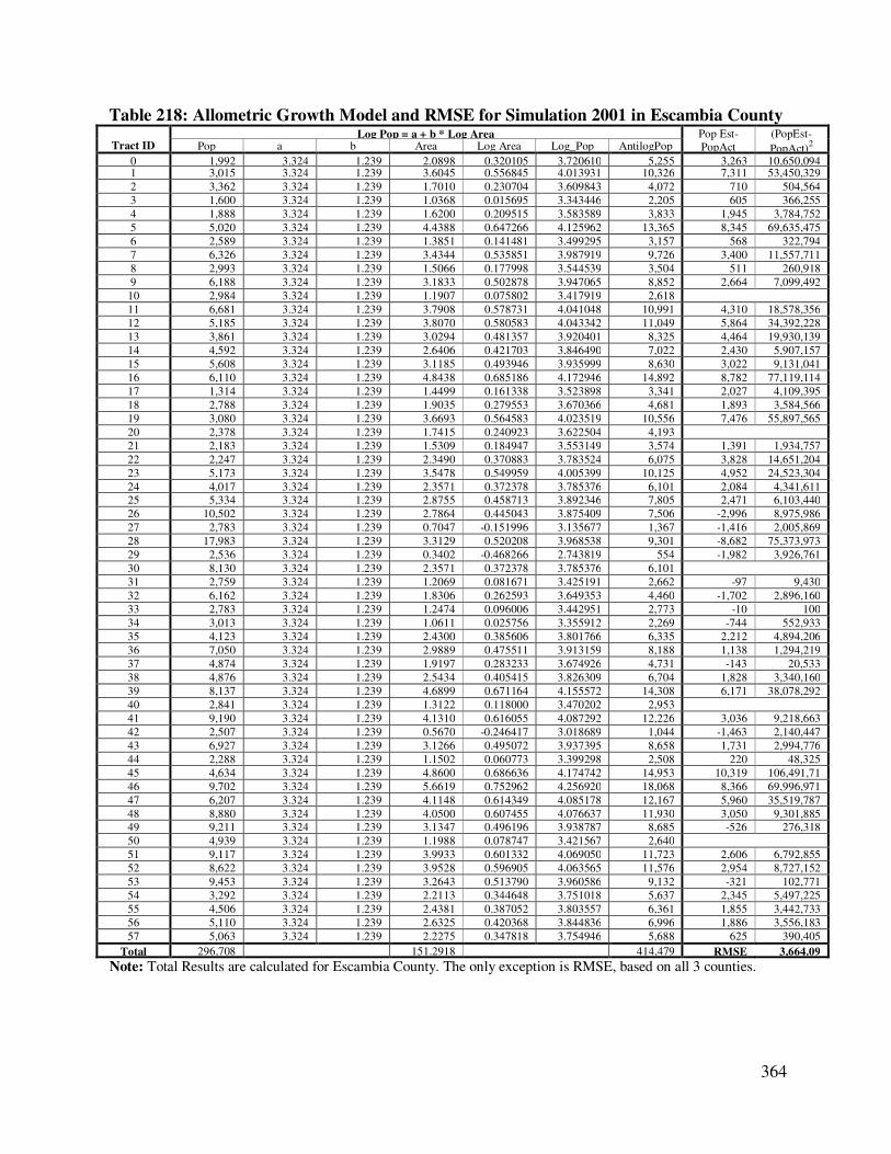
364
Table 218: Allometric Growth Model and RMSE for Simulation 2001 in Escambia County
Tract ID Log Pop = a + b * Log Area Pop Est-
PopAct
(PopEst-
PopAct)2 Pop a b Area Log Area Log_Pop AntilogPop
0 1,992 3.324 1.239 2.0898 0.320105 3.720610 5,255 3,263 10,650,094 1 3,015 3.324 1.239 3.6045 0.556845 4.013931 10,326 7,311 53,450,329
2 3,362 3.324 1.239 1.7010 0.230704 3.609843 4,072 710 504,564
3 1,600 3.324 1.239 1.0368 0.015695 3.343446 2,205 605 366,255
4 1,888 3.324 1.239 1.6200 0.209515 3.583589 3,833 1,945 3,784,752
5 5,020 3.324 1.239 4.4388 0.647266 4.125962 13,365 8,345 69,635,475
6 2,589 3.324 1.239 1.3851 0.141481 3.499295 3,157 568 322,794
7 6,326 3.324 1.239 3.4344 0.535851 3.987919 9,726 3,400 11,557,711
8 2,993 3.324 1.239 1.5066 0.177998 3.544539 3,504 511 260,918
9 6,188 3.324 1.239 3.1833 0.502878 3.947065 8,852 2,664 7,099,492
10 2,984 3.324 1.239 1.1907 0.075802 3.417919 2,618
11 6,681 3.324 1.239 3.7908 0.578731 4.041048 10,991 4,310 18,578,356
12 5,185 3.324 1.239 3.8070 0.580583 4.043342 11,049 5,864 34,392,228
13 3,861 3.324 1.239 3.0294 0.481357 3.920401 8,325 4,464 19,930,139
14 4,592 3.324 1.239 2.6406 0.421703 3.846490 7,022 2,430 5,907,157
15 5,608 3.324 1.239 3.1185 0.493946 3.935999 8,630 3,022 9,131,041
16 6,110 3.324 1.239 4.8438 0.685186 4.172946 14,892 8,782 77,119,114
17 1,314 3.324 1.239 1.4499 0.161338 3.523898 3,341 2,027 4,109,395
18 2,788 3.324 1.239 1.9035 0.279553 3.670366 4,681 1,893 3,584,566
19 3,080 3.324 1.239 3.6693 0.564583 4.023519 10,556 7,476 55,897,565
20 2,378 3.324 1.239 1.7415 0.240923 3.622504 4,193
21 2,183 3.324 1.239 1.5309 0.184947 3.553149 3,574 1,391 1,934,757
22 2,247 3.324 1.239 2.3490 0.370883 3.783524 6,075 3,828 14,651,204
23 5,173 3.324 1.239 3.5478 0.549959 4.005399 10,125 4,952 24,523,304
24 4,017 3.324 1.239 2.3571 0.372378 3.785376 6,101 2,084 4,341,611
25 5,334 3.324 1.239 2.8755 0.458713 3.892346 7,805 2,471 6,103,440
26 10,502 3.324 1.239 2.7864 0.445043 3.875409 7,506 -2,996 8,975,986
27 2,783 3.324 1.239 0.7047 -0.151996 3.135677 1,367 -1,416 2,005,869
28 17,983 3.324 1.239 3.3129 0.520208 3.968538 9,301 -8,682 75,373,973
29 2,536 3.324 1.239 0.3402 -0.468266 2.743819 554 -1,982 3,926,761
30 8,130 3.324 1.239 2.3571 0.372378 3.785376 6,101
31 2,759 3.324 1.239 1.2069 0.081671 3.425191 2,662 -97 9,430
32 6,162 3.324 1.239 1.8306 0.262593 3.649353 4,460 -1,702 2,896,160
33 2,783 3.324 1.239 1.2474 0.096006 3.442951 2,773 -10 100
34 3,013 3.324 1.239 1.0611 0.025756 3.355912 2,269 -744 552,933
35 4,123 3.324 1.239 2.4300 0.385606 3.801766 6,335 2,212 4,894,206
36 7,050 3.324 1.239 2.9889 0.475511 3.913159 8,188 1,138 1,294,219
37 4,874 3.324 1.239 1.9197 0.283233 3.674926 4,731 -143 20,533
38 4,876 3.324 1.239 2.5434 0.405415 3.826309 6,704 1,828 3,340,160
39 8,137 3.324 1.239 4.6899 0.671164 4.155572 14,308 6,171 38,078,292
40 2,841 3.324 1.239 1.3122 0.118000 3.470202 2,953
41 9,190 3.324 1.239 4.1310 0.616055 4.087292 12,226 3,036 9,218,663
42 2,507 3.324 1.239 0.5670 -0.246417 3.018689 1,044 -1,463 2,140,447
43 6,927 3.324 1.239 3.1266 0.495072 3.937395 8,658 1,731 2,994,776
44 2,288 3.324 1.239 1.1502 0.060773 3.399298 2,508 220 48,325
45 4,634 3.324 1.239 4.8600 0.686636 4.174742 14,953 10,319 106,491,71
46 9,702 3.324 1.239 5.6619 0.752962 4.256920 18,068 8,366 69,996,971
47 6,207 3.324 1.239 4.1148 0.614349 4.085178 12,167 5,960 35,519,787
48 8,880 3.324 1.239 4.0500 0.607455 4.076637 11,930 3,050 9,301,885
49 9,211 3.324 1.239 3.1347 0.496196 3.938787 8,685 -526 276,318
50 4,939 3.324 1.239 1.1988 0.078747 3.421567 2,640
51 9,117 3.324 1.239 3.9933 0.601332 4.069050 11,723 2,606 6,792,855
52 8,622 3.324 1.239 3.9528 0.596905 4.063565 11,576 2,954 8,727,152
53 9,453 3.324 1.239 3.2643 0.513790 3.960586 9,132 -321 102,771
54 3,292 3.324 1.239 2.2113 0.344648 3.751018 5,637 2,345 5,497,225
55 4,506 3.324 1.239 2.4381 0.387052 3.803557 6,361 1,855 3,442,733
56 5,110 3.324 1.239 2.6325 0.420368 3.844836 6,996 1,886 3,556,183
57 5,063 3.324 1.239 2.2275 0.347818 3.754946 5,688 625 390,405
Total 296,708 151.2918 414,479 RMSE 3,664.09
Note: Total Results are calculated for Escambia County. The only exception is RMSE, based on all 3 counties.

365
Table 219: Allometric Growth Model and RMSE for Simulation 2001 in Sta. Rosa County
Tract ID Log Pop = a + b * Log Area Pop Est-
PopAct
(PopEst-
PopAct)2 Pop a b Area Log Area Log_Pop AntilogPop
91 3,658 3.324 1.239 2.0574 0.313319 3.712202 5,155 1,497 2,240,058 92 4,167 3.324 1.239 2.5353 0.404029 3.824592 6,677 2,510 6,300,949
93 6,846 3.324 1.239 1.1664 0.066848 3.406824 2,552 -4,294 18,441,292
94 2,213 3.324 1.239 1.4580 0.163758 3.526896 3,364 1,151 1,325,507
95 8,296 3.324 1.239 3.4425 0.536874 3.989187 9,754 1,458 2,126,031
96 6,234 3.324 1.239 1.8711 0.272097 3.661128 4,583 -1,651 2,726,556
97 6,118 3.324 1.239 4.9977 0.698770 4.189776 15,480 9,362 87,650,581
98 5,029 3.324 1.239 1.6200 0.209515 3.583589 3,833 -1,196 1,429,355
99 8,390 3.324 1.239 2.4300 0.385606 3.801766 6,335 -2,055 4,221,853
100 3,698 3.324 1.239 1.9035 0.279553 3.670366 4,681
101 3,213 3.324 1.239 2.2113 0.344648 3.751018 5,637 2,424 5,873,915
102 6,925 3.324 1.239 3.6450 0.561698 4.019943 10,470 3,545 12,566,437
103 10,546 3.324 1.239 3.8313 0.583346 4.046766 11,137 591 349,210
104 3,903 3.324 1.239 0.5589 -0.252666 3.010947 1,026 -2,877 8,279,853
105 9,054 3.324 1.239 2.1465 0.331731 3.735015 5,433 -3,621 13,113,918
106 10,209 3.324 1.239 1.3608 0.133794 3.489771 3,089 -7,120 50,699,137
107 7,875 3.324 1.239 1.3041 0.115311 3.466870 2,930 -4,945 24,452,853
108 9,276 3.324 1.239 1.1340 0.054613 3.391666 2,464 -6,812 46,401,422
109 5,722 3.324 1.239 2.1870 0.339849 3.745073 5,560 -162 26,253
Total 121,372 41.8608 110,159 RMSE 3,664.09
Note: Total Results are calculated for Santa Rosa County. The only exception is RMSE, based on all 3 counties.
Table 220: Allometric Growth Model and RMSE for Simulation 2001 in Okaloosa County
Tract ID Log Pop = a + b * Log Area Pop Est-
PopAct
(PopEst-
PopAct)2 Pop a b Area Log Area Log_Pop AntilogPop
58 6,841 3.324 1.239 2.0331 0.308159 3.705809 5,079 -1,762 3,103,388 59 1,817 3.324 1.239 0.8262 -0.082915 3.221269 1,664 -153 23,274
60 8,713 3.324 1.239 2.3895 0.378307 3.792722 6,205
61 5,608 3.324 1.239 3.4182 0.533797 3.985375 9,669 4,061 16,490,547
62 5,542 3.324 1.239 3.9042 0.591532 4.056908 11,400 5,858 34,317,200
63 5,490 3.324 1.239 1.7172 0.234821 3.614943 4,120 -1,370 1,875,708
64 7,988 3.324 1.239 2.7783 0.443779 3.873842 7,479 -509 259,102
65 5,468 3.324 1.239 1.7334 0.238899 3.619996 4,169 -1,299 1,688,306
66 4,669 3.324 1.239 1.3365 0.125969 3.480076 3,020 -1,649 2,717,628
67 10,061 3.324 1.239 1.4661 0.166164 3.529877 3,387 -6,674 44,535,874
68 3,345 3.324 1.239 2.2356 0.349394 3.756899 5,713 2,368 5,609,609
69 7,348 3.324 1.239 2.5029 0.398443 3.817671 6,572 -776 602,788
70 7,562 3.324 1.239 2.5515 0.406796 3.828020 6,730
71 7,388 3.324 1.239 1.5309 0.184947 3.553149 3,574 -3,814 14,546,937
72 8,015 3.324 1.239 3.2157 0.507276 3.952514 8,964 949 901,092
73 1,855 3.324 1.239 0.7857 -0.104743 3.194223 1,564 -291 84,710
74 2,665 3.324 1.239 1.1259 0.051500 3.387808 2,442 -223 49,572
75 5,439 3.324 1.239 0.8910 -0.050122 3.261898 1,828 -3,611 13,041,683
76 5,242 3.324 1.239 1.5390 0.187239 3.555989 3,597 -1,645 2,704,711
77 6,388 3.324 1.239 2.3247 0.366367 3.777929 5,997 -391 152,940
78 7,062 3.324 1.239 3.3048 0.519145 3.967221 9,273 2,211 4,888,580
79 3,233 3.324 1.239 1.6443 0.215981 3.591601 3,905 672 451,336
80 2,360 3.324 1.239 1.4985 0.175657 3.541639 3,480
81 4,068 3.324 1.239 2.3652 0.373868 3.787222 6,127 2,059 4,237,995
82 4,111 3.324 1.239 2.9889 0.475511 3.913159 8,188 4,077 16,618,973
83 2,901 3.324 1.239 1.8063 0.256790 3.642163 4,387 1,486 2,208,047
84 3,715 3.324 1.239 2.2680 0.355643 3.764642 5,816 2,101 4,415,177
85 2,067 3.324 1.239 0.9963 -0.001610 3.322005 2,099 32 1,022
86 4,202 3.324 1.239 2.6892 0.429623 3.856303 7,183 2,981 8,886,081
87 7,605 3.324 1.239 2.4381 0.387052 3.803557 6,361 -1,244 1,546,391
88 1,844 3.324 1.239 0.9153 -0.038437 3.276377 1,890 46 2,082
89 9,574 3.324 1.239 1.8792 0.273973 3.663453 4,607 -4,967 24,667,470
90 3,264 3.324 1.239 1.7658 0.246942 3.629961 4,265
Total 173,450 66.8655 170,757 RMSE 3,664.09
Note: Total Results are calculated for Okaloosa County. The only exception is RMSE, based on all 3 counties.
TOTAL Pop
Area
AntilogPop SIM 2001 591,530 260.0181 695,395 RMSE 3,664.09

366
Table 221: Allometric Growth Model and RMSE for Simulation 2005 Smart in Escambia
Tract ID Log Pop = a + b * Log Area Pop Est-
PopAct
(PopEst-
PopAct)2 Pop a b Area Log Area Log_Pop AntilogPop
0 1,864 3.451 0.733 1.6605 0.220239 3.612435 4,097 2,233 4,984,989 1 2,872 3.451 0.733 2.6973 0.430929 3.766871 5,846 2,974 8,845,663
2 3,178 3.451 0.733 1.3041 0.115311 3.535523 3,432 254 64,418
3 1,534 3.451 0.733 0.7938 -0.100289 3.377488 2,385 851 724,200
4 1,737 3.451 0.733 1.3203 0.120673 3.539453 3,463 1,726 2,979,091
5 4,744 3.451 0.733 3.3129 0.520208 3.832313 6,797 2,053 4,214,516
6 2,494 3.451 0.733 1.0368 0.015695 3.462504 2,901 407 165,414
7 6,328 3.451 0.733 2.4786 0.394206 3.739953 5,495 -833 694,192
8 2,977 3.451 0.733 1.1016 0.042024 3.481804 3,033 56 3,082
9 6,378 3.451 0.733 2.2842 0.358734 3.713952 5,175 -1,203 1,446,012
10 3,055 3.451 0.733 0.9234 -0.034610 3.425631 2,665
11 6,853 3.451 0.733 2.7054 0.432231 3.767826 5,859 -994 987,978
12 5,162 3.451 0.733 2.8755 0.458713 3.787237 6,127 965 930,926
13 3,837 3.451 0.733 2.0979 0.321785 3.686868 4,863 1,026 1,051,848
14 4,455 3.451 0.733 1.7739 0.248929 3.633465 4,300 -155 24,035
15 5,756 3.451 0.733 2.3247 0.366367 3.719547 5,243 -513 263,577
16 6,170 3.451 0.733 3.8394 0.584263 3.879265 7,573 1,403 1,968,266
17 1,209 3.451 0.733 1.1178 0.048364 3.486451 3,065 1,856 3,445,271
18 2,695 3.451 0.733 1.4499 0.161338 3.569261 3,709 1,014 1,028,265
19 2,934 3.451 0.733 2.5353 0.404029 3.747154 5,587 2,653 7,036,692
20 2,230 3.451 0.733 1.3365 0.125969 3.543335 3,494
21 2,093 3.451 0.733 1.1259 0.051500 3.488749 3,081 988 976,953
22 2,136 3.451 0.733 1.4904 0.173303 3.578031 3,785 1,649 2,718,198
23 5,001 3.451 0.733 2.5596 0.408172 3.750190 5,626 625 390,470
24 3,809 3.451 0.733 1.5876 0.200741 3.598143 3,964 155 24,052
25 5,139 3.451 0.733 1.7415 0.240923 3.627597 4,242 -897 804,149
26 10,865 3.451 0.733 3.3939 0.530699 3.840002 6,918 -3,947 15,576,063
27 2,945 3.451 0.733 2.0898 0.320105 3.685637 4,849 1,904 3,624,560
28 20,066 3.451 0.733 9.3393 0.970314 4.162240 14,529 -5,537 30,656,636
29 2,654 3.451 0.733 0.8424 -0.074482 3.396405 2,491 -163 26,511
30 8,536 3.451 0.733 3.0132 0.479028 3.802127 6,341
31 2,778 3.451 0.733 1.2798 0.107142 3.529535 3,385 607 368,227
32 6,370 3.451 0.733 1.7253 0.236865 3.624622 4,213 -2,157 4,651,381
33 2,797 3.451 0.733 0.8262 -0.082915 3.390223 2,456 -341 116,300
34 3,005 3.451 0.733 1.1178 0.048364 3.486451 3,065 60 3,617
35 3,958 3.451 0.733 1.6686 0.222352 3.613984 4,111 153 23,515
36 6,939 3.451 0.733 2.1303 0.328441 3.691747 4,918 -2,021 4,086,338
37 4,778 3.451 0.733 1.3689 0.136372 3.550960 3,556 -1,222 1,493,310
38 4,951 3.451 0.733 2.1951 0.341454 3.701286 5,027 76 5,736
39 8,293 3.451 0.733 4.6737 0.669661 3.941861 8,747 454 206,157
40 3,024 3.451 0.733 1.0611 0.025756 3.469879 2,950
41 9,720 3.451 0.733 4.1472 0.617755 3.903814 8,013 -1,707 2,912,636
42 2,672 3.451 0.733 0.8181 -0.087194 3.387087 2,438 -234 54,616
43 7,284 3.451 0.733 3.0051 0.477859 3.801271 6,328 -956 913,821
44 2,383 3.451 0.733 0.9315 -0.030817 3.428411 2,682 299 89,225
45 4,557 3.451 0.733 3.6531 0.562662 3.863431 7,302 2,745 7,534,018
46 10,109 3.451 0.733 3.8475 0.585179 3.879936 7,585 -2,524 6,372,309
47 6,437 3.451 0.733 2.9970 0.476687 3.800411 6,316 -121 14,749
48 9,202 3.451 0.733 2.8188 0.450064 3.780897 6,038 -3,164 10,010,544
49 9,930 3.451 0.733 2.6244 0.419030 3.758149 5,730 -4,200 17,640,622
50 5,300 3.451 0.733 1.1907 0.075802 3.506563 3,210
51 9,963 3.451 0.733 4.0986 0.612636 3.900062 7,944 -2,019 4,074,691
52 9,406 3.451 0.733 3.4587 0.538913 3.846023 7,015 -2,391 5,717,230
53 10,209 3.451 0.733 2.8431 0.453792 3.783630 6,076 -4,133 17,080,316
54 3,173 3.451 0.733 2.1222 0.326786 3.690534 4,904 1,731 2,995,732
55 4,548 3.451 0.733 1.2474 0.096006 3.521372 3,322 -1,226 1,503,590
56 5,111 3.451 0.733 1.4175 0.151523 3.562066 3,648 -1,463 2,140,084
57 5,018 3.451 0.733 1.7091 0.232767 3.621619 4,184 -834 695,124
Total 303,621 129.1302 286,097 RMSE 2,006.31
Note: Total Results are calculated for Escambia County. The only exception is RMSE, based on all 3 counties.
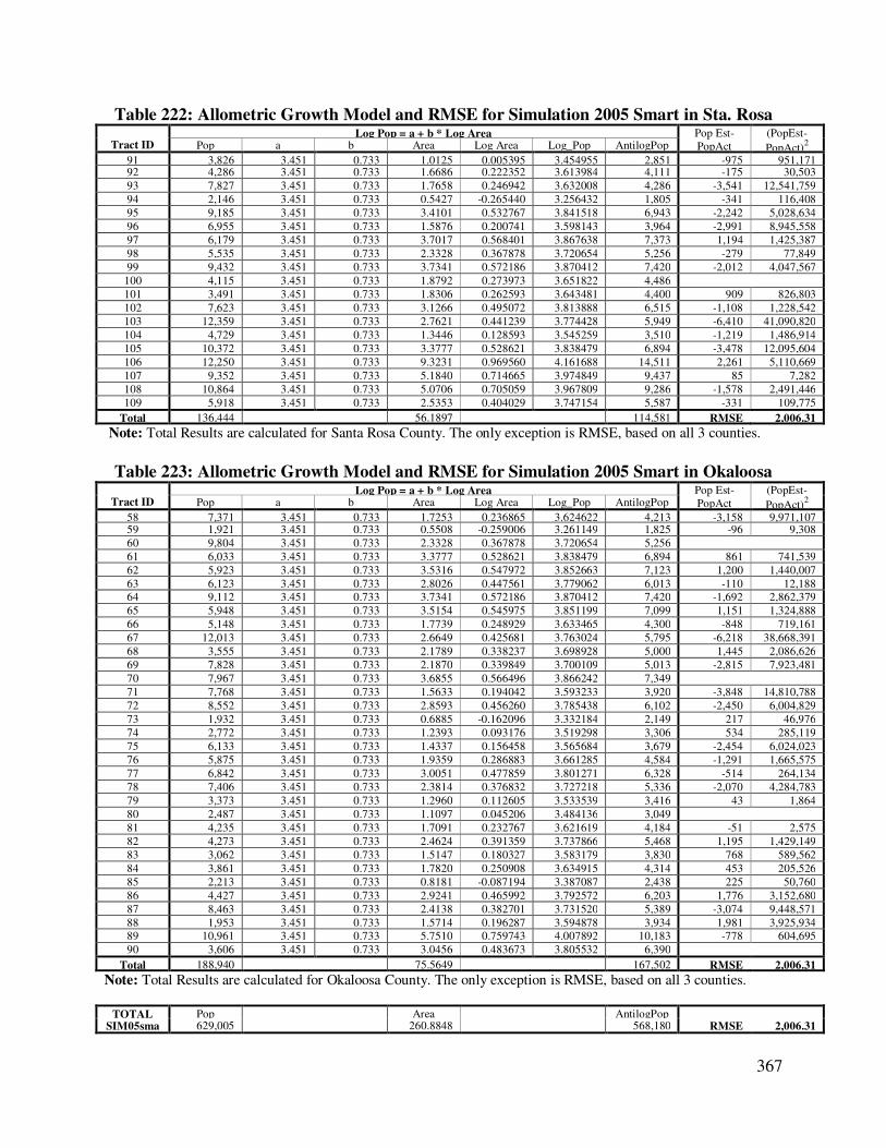
367
Table 222: Allometric Growth Model and RMSE for Simulation 2005 Smart in Sta. Rosa
Tract ID Log Pop = a + b * Log Area Pop Est-
PopAct
(PopEst-
PopAct)2 Pop a b Area Log Area Log_Pop AntilogPop
91 3,826 3.451 0.733 1.0125 0.005395 3.454955 2,851 -975 951,171 92 4,286 3.451 0.733 1.6686 0.222352 3.613984 4,111 -175 30,503
93 7,827 3.451 0.733 1.7658 0.246942 3.632008 4,286 -3,541 12,541,759
94 2,146 3.451 0.733 0.5427 -0.265440 3.256432 1,805 -341 116,408
95 9,185 3.451 0.733 3.4101 0.532767 3.841518 6,943 -2,242 5,028,634
96 6,955 3.451 0.733 1.5876 0.200741 3.598143 3,964 -2,991 8,945,558
97 6,179 3.451 0.733 3.7017 0.568401 3.867638 7,373 1,194 1,425,387
98 5,535 3.451 0.733 2.3328 0.367878 3.720654 5,256 -279 77,849
99 9,432 3.451 0.733 3.7341 0.572186 3.870412 7,420 -2,012 4,047,567
100 4,115 3.451 0.733 1.8792 0.273973 3.651822 4,486
101 3,491 3.451 0.733 1.8306 0.262593 3.643481 4,400 909 826,803
102 7,623 3.451 0.733 3.1266 0.495072 3.813888 6,515 -1,108 1,228,542
103 12,359 3.451 0.733 2.7621 0.441239 3.774428 5,949 -6,410 41,090,820
104 4,729 3.451 0.733 1.3446 0.128593 3.545259 3,510 -1,219 1,486,914
105 10,372 3.451 0.733 3.3777 0.528621 3.838479 6,894 -3,478 12,095,604
106 12,250 3.451 0.733 9.3231 0.969560 4.161688 14,511 2,261 5,110,669
107 9,352 3.451 0.733 5.1840 0.714665 3.974849 9,437 85 7,282
108 10,864 3.451 0.733 5.0706 0.705059 3.967809 9,286 -1,578 2,491,446
109 5,918 3.451 0.733 2.5353 0.404029 3.747154 5,587 -331 109,775
Total 136,444 56.1897 114,581 RMSE 2,006.31
Note: Total Results are calculated for Santa Rosa County. The only exception is RMSE, based on all 3 counties.
Table 223: Allometric Growth Model and RMSE for Simulation 2005 Smart in Okaloosa
Tract ID Log Pop = a + b * Log Area Pop Est-
PopAct
(PopEst-
PopAct)2 Pop a b Area Log Area Log_Pop AntilogPop
58 7,371 3.451 0.733 1.7253 0.236865 3.624622 4,213 -3,158 9,971,107 59 1,921 3.451 0.733 0.5508 -0.259006 3.261149 1,825 -96 9,308
60 9,804 3.451 0.733 2.3328 0.367878 3.720654 5,256
61 6,033 3.451 0.733 3.3777 0.528621 3.838479 6,894 861 741,539
62 5,923 3.451 0.733 3.5316 0.547972 3.852663 7,123 1,200 1,440,007
63 6,123 3.451 0.733 2.8026 0.447561 3.779062 6,013 -110 12,188
64 9,112 3.451 0.733 3.7341 0.572186 3.870412 7,420 -1,692 2,862,379
65 5,948 3.451 0.733 3.5154 0.545975 3.851199 7,099 1,151 1,324,888
66 5,148 3.451 0.733 1.7739 0.248929 3.633465 4,300 -848 719,161
67 12,013 3.451 0.733 2.6649 0.425681 3.763024 5,795 -6,218 38,668,391
68 3,555 3.451 0.733 2.1789 0.338237 3.698928 5,000 1,445 2,086,626
69 7,828 3.451 0.733 2.1870 0.339849 3.700109 5,013 -2,815 7,923,481
70 7,967 3.451 0.733 3.6855 0.566496 3.866242 7,349
71 7,768 3.451 0.733 1.5633 0.194042 3.593233 3,920 -3,848 14,810,788
72 8,552 3.451 0.733 2.8593 0.456260 3.785438 6,102 -2,450 6,004,829
73 1,932 3.451 0.733 0.6885 -0.162096 3.332184 2,149 217 46,976
74 2,772 3.451 0.733 1.2393 0.093176 3.519298 3,306 534 285,119
75 6,133 3.451 0.733 1.4337 0.156458 3.565684 3,679 -2,454 6,024,023
76 5,875 3.451 0.733 1.9359 0.286883 3.661285 4,584 -1,291 1,665,575
77 6,842 3.451 0.733 3.0051 0.477859 3.801271 6,328 -514 264,134
78 7,406 3.451 0.733 2.3814 0.376832 3.727218 5,336 -2,070 4,284,783
79 3,373 3.451 0.733 1.2960 0.112605 3.533539 3,416 43 1,864
80 2,487 3.451 0.733 1.1097 0.045206 3.484136 3,049
81 4,235 3.451 0.733 1.7091 0.232767 3.621619 4,184 -51 2,575
82 4,273 3.451 0.733 2.4624 0.391359 3.737866 5,468 1,195 1,429,149
83 3,062 3.451 0.733 1.5147 0.180327 3.583179 3,830 768 589,562
84 3,861 3.451 0.733 1.7820 0.250908 3.634915 4,314 453 205,526
85 2,213 3.451 0.733 0.8181 -0.087194 3.387087 2,438 225 50,760
86 4,427 3.451 0.733 2.9241 0.465992 3.792572 6,203 1,776 3,152,680
87 8,463 3.451 0.733 2.4138 0.382701 3.731520 5,389 -3,074 9,448,571
88 1,953 3.451 0.733 1.5714 0.196287 3.594878 3,934 1,981 3,925,934
89 10,961 3.451 0.733 5.7510 0.759743 4.007892 10,183 -778 604,695
90 3,606 3.451 0.733 3.0456 0.483673 3.805532 6,390
Total 188,940 75.5649 167,502 RMSE 2,006.31
Note: Total Results are calculated for Okaloosa County. The only exception is RMSE, based on all 3 counties.
TOTAL Pop
Area
AntilogPop SIM05sma 629,005 260.8848 568,180 RMSE 2,006.31

368
Table 224: Allometric Growth Model and RMSE for Simulation 2005 Normal in Escambia
Tract ID Log Pop = a + b * Log Area Pop Est-
PopAct
(PopEst-
PopAct)2 Pop a b Area Log Area Log_Pop AntilogPop
0 1,864 3.466 0.748 1.7172 0.234821 3.641646 4,382 2,518 6,338,985 1 2,872 3.466 0.748 2.8107 0.448814 3.801713 6,335 3,463 11,988,997
2 3,178 3.466 0.748 1.3284 0.123329 3.558250 3,616 438 192,001
3 1,534 3.466 0.748 0.7857 -0.104743 3.387652 2,441 907 823,509
4 1,737 3.466 0.748 1.3365 0.125969 3.560225 3,633 1,896 3,593,528
5 4,744 3.466 0.748 3.3696 0.527578 3.860629 7,255 2,511 6,304,382
6 2,494 3.466 0.748 1.0935 0.038819 3.495036 3,126 632 399,856
7 6,328 3.466 0.748 2.6406 0.421703 3.781434 6,046 -282 79,796
8 2,977 3.466 0.748 1.1340 0.054613 3.506851 3,213 236 55,486
9 6,378 3.466 0.748 2.3409 0.369383 3.742298 5,525 -853 728,345
10 3,055 3.466 0.748 0.9558 -0.019633 3.451315 2,827
11 6,853 3.466 0.748 2.7864 0.445043 3.798893 6,294 -559 313,036
12 5,162 3.466 0.748 2.9646 0.471966 3.819031 6,592 1,430 2,045,484
13 3,837 3.466 0.748 2.1789 0.338237 3.719001 5,236 1,399 1,957,264
14 4,455 3.466 0.748 1.8306 0.262593 3.662420 4,596 141 20,000
15 5,756 3.466 0.748 2.3328 0.367878 3.741172 5,510 -246 60,386
16 6,170 3.466 0.748 4.0500 0.607455 3.920376 8,325 2,155 4,643,374
17 1,209 3.466 0.748 1.1745 0.069853 3.518250 3,298 2,089 4,363,902
18 2,695 3.466 0.748 1.4823 0.170936 3.593860 3,925 1,230 1,513,357
19 2,934 3.466 0.748 2.6406 0.421703 3.781434 6,046 3,112 9,681,548
20 2,230 3.466 0.748 1.3770 0.138934 3.569923 3,715
21 2,093 3.466 0.748 1.1583 0.063821 3.513738 3,264 1,171 1,371,030
22 2,136 3.466 0.748 1.5390 0.187239 3.606054 4,037 1,901 3,613,650
23 5,001 3.466 0.748 2.6487 0.423033 3.782429 6,059 1,058 1,120,178
24 3,809 3.466 0.748 1.6524 0.218115 3.629150 4,257 448 201,113
25 5,139 3.466 0.748 1.7577 0.244945 3.649219 4,459 -680 462,663
26 10,865 3.466 0.748 3.4425 0.536874 3.867582 7,372 -3,493 12,201,477
27 2,945 3.466 0.748 2.1951 0.341454 3.721408 5,265 2,320 5,382,931
28 20,066 3.466 0.748 9.8577 0.993776 4.209344 16,194 -3,872 14,995,268
29 2,654 3.466 0.748 0.8586 -0.066209 3.416476 2,609 -45 2,024
30 8,536 3.466 0.748 3.1023 0.491684 3.833779 6,820
31 2,778 3.466 0.748 1.3041 0.115311 3.552253 3,567 789 621,866
32 6,370 3.466 0.748 1.7982 0.254838 3.656619 4,535 -1,835 3,365,634
33 2,797 3.466 0.748 0.8667 -0.062131 3.419526 2,627 -170 28,765
34 3,005 3.466 0.748 1.1421 0.057704 3.509163 3,230 225 50,492
35 3,958 3.466 0.748 1.6929 0.228631 3.637016 4,335 377 142,333
36 6,939 3.466 0.748 2.2113 0.344648 3.723796 5,294 -1,645 2,705,523
37 4,778 3.466 0.748 1.4337 0.156458 3.583031 3,829 -949 901,514
38 4,951 3.466 0.748 2.3328 0.367878 3.741172 5,510 559 312,776
39 8,293 3.466 0.748 4.7871 0.680072 3.974694 9,434 1,141 1,301,800
40 3,024 3.466 0.748 1.1421 0.057704 3.509163 3,230
41 9,720 3.466 0.748 4.3578 0.639267 3.944172 8,794 -926 858,021
42 2,672 3.466 0.748 0.8586 -0.066209 3.416476 2,609 -63 3,968
43 7,284 3.466 0.748 3.0456 0.483673 3.827787 6,726 -558 310,838
44 2,383 3.466 0.748 0.9963 -0.001610 3.464796 2,916 533 284,148
45 4,557 3.466 0.748 3.8232 0.582427 3.901655 7,974 3,417 11,673,276
46 10,109 3.466 0.748 4.1472 0.617755 3.928081 8,474 -1,635 2,673,719
47 6,437 3.466 0.748 3.1185 0.493946 3.835471 6,847 410 167,726
48 9,202 3.466 0.748 2.8836 0.459935 3.810031 6,457 -2,745 7,534,976
49 9,930 3.466 0.748 2.7459 0.438685 3.794136 6,225 -3,705 13,727,364
50 5,300 3.466 0.748 1.1988 0.078747 3.524903 3,349
51 9,963 3.466 0.748 4.2282 0.626156 3.934364 8,597 -1,366 1,865,015
52 9,406 3.466 0.748 3.6288 0.559763 3.884703 7,668 -1,738 3,019,377
53 10,209 3.466 0.748 2.9565 0.470778 3.818142 6,579 -3,630 13,178,883
54 3,173 3.466 0.748 2.2194 0.346236 3.724984 5,309 2,136 4,561,007
55 4,548 3.466 0.748 1.2879 0.109882 3.548192 3,533 -1,015 1,029,429
56 5,111 3.466 0.748 1.4742 0.168556 3.592080 3,909 -1,202 1,444,490
57 5,018 3.466 0.748 1.7739 0.248929 3.652199 4,490 -528 279,301
Total 303,621 133.9983 308,316 RMSE 1,884.30
Note: Total Results are calculated for Escambia County. The only exception is RMSE, based on all 3 counties.

369
Table 225: Allometric Growth Model and RMSE for Simulation 2005 Normal in Sta. Rosa
Tract ID Log Pop = a + b * Log Area Pop Est-
PopAct
(PopEst-
PopAct)2 Pop a b Area Log Area Log_Pop AntilogPop
91 3,826 3.466 0.748 1.1421 0.057704 3.509163 3,230 -596 355,569 92 4,286 3.466 0.748 1.7901 0.252877 3.655152 4,520 234 54,823
93 7,827 3.466 0.748 1.8711 0.272097 3.669529 4,672 -3,155 9,952,279
94 2,146 3.466 0.748 0.5832 -0.234182 3.290832 1,954 -192 37,025
95 9,185 3.466 0.748 3.5964 0.555868 3.881789 7,617 -1,568 2,458,332
96 6,955 3.466 0.748 1.6281 0.211681 3.624337 4,211 -2,744 7,532,079
97 6,179 3.466 0.748 3.8313 0.583346 3.902343 7,986 1,807 3,266,154
98 5,535 3.466 0.748 2.5110 0.399847 3.765085 5,822 287 82,470
99 9,432 3.466 0.748 3.8718 0.587913 3.905759 8,049 -1,383 1,911,821
100 4,115 3.466 0.748 1.9521 0.290502 3.683296 4,823
101 3,491 3.466 0.748 1.8711 0.272097 3.669529 4,672 1,181 1,395,415
102 7,623 3.466 0.748 3.3129 0.520208 3.855116 7,163 -460 211,283
103 12,359 3.466 0.748 3.0537 0.484826 3.828650 6,740 -5,619 31,574,865
104 4,729 3.466 0.748 1.4256 0.153998 3.581190 3,812 -917 840,287
105 10,372 3.466 0.748 3.5316 0.547972 3.875883 7,514 -2,858 8,167,027
106 12,250 3.466 0.748 9.6552 0.984761 4.202601 15,944 3,694 13,646,761
107 9,352 3.466 0.748 5.4027 0.732611 4.013993 10,327 975 951,494
108 10,864 3.466 0.748 5.3865 0.731307 4.013017 10,304 -560 313,294
109 5,918 3.466 0.748 2.6811 0.428313 3.786378 6,115 197 38,707
Total 136,444 59.0976 125,476 RMSE 1,884.30
Note: Total Results are calculated for Santa Rosa County. The only exception is RMSE, based on all 3 counties.
Table 226: Allometric Growth Model and RMSE for Simulation 2005 Normal in Okaloosa
Tract ID Log Pop = a + b * Log Area Pop Est-
PopAct
(PopEst-
PopAct)2 Pop a b Area Log Area Log_Pop AntilogPop
58 7,371 3.466 0.748 1.8468 0.266420 3.665282 4,627 -2,744 7,530,556 59 1,921 3.466 0.748 0.5832 -0.234182 3.290832 1,954 33 1,062
60 9,804 3.466 0.748 2.5029 0.398443 3.764036 5,808
61 6,033 3.466 0.748 3.4992 0.543969 3.872889 7,463 1,430 2,043,681
62 5,923 3.466 0.748 3.7017 0.568401 3.891164 7,783 1,860 3,460,739
63 6,123 3.466 0.748 2.9241 0.465992 3.814562 6,525 402 161,383
64 9,112 3.466 0.748 3.9447 0.596014 3.911818 8,162 -950 901,719
65 5,948 3.466 0.748 3.5640 0.551938 3.878849 7,566 1,618 2,616,969
66 5,148 3.466 0.748 1.8549 0.268321 3.666704 4,642 -506 256,051
67 12,013 3.466 0.748 2.7783 0.443779 3.797947 6,280 -5,733 32,869,419
68 3,555 3.466 0.748 2.2356 0.349394 3.727347 5,338 1,783 3,177,696
69 7,828 3.466 0.748 2.3004 0.361803 3.736629 5,453 -2,375 5,641,018
70 7,967 3.466 0.748 3.7341 0.572186 3.893995 7,834
71 7,768 3.466 0.748 1.6200 0.209515 3.622717 4,195 -3,573 12,767,346
72 8,552 3.466 0.748 2.9727 0.473151 3.819917 6,606 -1,946 3,788,192
73 1,932 3.466 0.748 0.7695 -0.113791 3.380884 2,404 472 222,521
74 2,772 3.466 0.748 1.3203 0.120673 3.556263 3,600 828 685,044
75 6,133 3.466 0.748 1.4661 0.166164 3.590290 3,893 -2,240 5,017,360
76 5,875 3.466 0.748 2.0250 0.306425 3.695206 4,957 -918 842,996
77 6,842 3.466 0.748 3.1023 0.491684 3.833779 6,820 -22 487
78 7,406 3.466 0.748 2.4624 0.391359 3.758736 5,738 -1,668 2,783,296
79 3,373 3.466 0.748 1.3365 0.125969 3.560225 3,633 260 67,423
80 2,487 3.466 0.748 1.1745 0.069853 3.518250 3,298
81 4,235 3.466 0.748 1.7739 0.248929 3.652199 4,490 255 64,776
82 4,273 3.466 0.748 2.5272 0.402640 3.767174 5,850 1,577 2,487,718
83 3,062 3.466 0.748 1.5228 0.182643 3.602617 4,005 943 889,499
84 3,861 3.466 0.748 1.8468 0.266420 3.665282 4,627 766 586,471
85 2,213 3.466 0.748 0.8019 -0.095880 3.394282 2,479 266 70,772
86 4,427 3.466 0.748 2.9970 0.476687 3.822562 6,646 2,219 4,924,052
87 8,463 3.466 0.748 2.5515 0.406796 3.770283 5,892 -2,571 6,608,621
88 1,953 3.466 0.748 1.6443 0.215981 3.627554 4,242 2,289 5,238,768
89 10,961 3.466 0.748 6.0345 0.780641 4.049920 11,218 257 66,105
90 3,606 3.466 0.748 3.1023 0.491684 3.833779 6,820
Total 188,940 78.5214 180,845 RMSE 1,884.30
Note: Total Results are calculated for Okaloosa County. The only exception is RMSE, based on all 3 counties.
TOTAL Pop
Area
AntilogPop SIM05norm 629,005 271.6173 614,638 RMSE 1,884.30
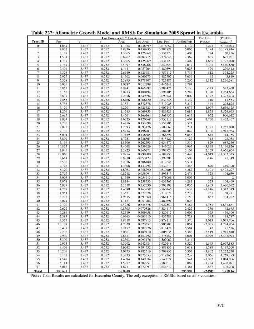
370
Table 227: Allometric Growth Model and RMSE for Simulation 2005 Sprawl in Escambia
Tract ID Log Pop = a + b * Log Area Pop Est-
PopAct
(PopEst-
PopAct)2 Pop a b Area Log Area Log_Pop AntilogPop
0 1,864 3.437 0.752 1.7334 0.238899 3.616652 4,137 2,273 5,165,073 1 2,872 3.437 0.752 2.8836 0.459935 3.782871 6,066 3,194 10,198,846
2 3,178 3.437 0.752 1.3365 0.125969 3.531729 3,402 224 50,156
3 1,534 3.437 0.752 0.8262 -0.082915 3.374648 2,369 835 697,981
4 1,737 3.437 0.752 1.3365 0.125969 3.531729 3,402 1,665 2,772,078
5 4,744 3.437 0.752 3.5397 0.548966 3.849823 7,077 2,333 5,440,880
6 2,494 3.437 0.752 1.1421 0.057704 3.480394 3,023 529 279,512
7 6,328 3.437 0.752 2.6649 0.425681 3.757112 5,716 -612 374,225
8 2,977 3.437 0.752 1.1502 0.060773 3.482702 3,039 62 3,819
9 6,378 3.437 0.752 2.3895 0.378307 3.721487 5,266 -1,112 1,236,381
10 3,055 3.437 0.752 1.0287 0.012289 3.446241 2,794
11 6,853 3.437 0.752 2.9241 0.465992 3.787426 6,130 -723 523,430
12 5,162 3.437 0.752 3.0213 0.480194 3.798106 6,282 1,120 1,254,654
13 3,837 3.437 0.752 2.2356 0.349394 3.699744 5,009 1,172 1,373,404
14 4,455 3.437 0.752 1.8468 0.266420 3.637348 4,339 -116 13,553
15 5,756 3.437 0.752 2.3571 0.372378 3.717028 5,212 -544 295,625
16 6,170 3.437 0.752 4.2201 0.625323 3.907243 8,077 1,907 3,636,125
17 1,209 3.437 0.752 1.1745 0.069853 3.489529 3,087 1,878 3,526,693
18 2,695 3.437 0.752 1.4661 0.166164 3.561955 3,647 952 906,612
19 2,934 3.437 0.752 2.6325 0.420368 3.753117 5,664 2,730 7,452,457
20 2,230 3.437 0.752 1.4256 0.153998 3.552806 3,571
21 2,093 3.437 0.752 1.2393 0.093176 3.507069 3,214 1,121 1,257,020
22 2,136 3.437 0.752 1.5714 0.196287 3.584608 3,842 1,706 2,911,954
23 5,001 3.437 0.752 2.7459 0.438685 3.766891 5,846 845 714,755
24 3,809 3.437 0.752 1.7253 0.236865 3.615122 4,122 313 98,053
25 5,139 3.437 0.752 1.8306 0.262593 3.634470 4,310 -829 687,356
26 10,865 3.437 0.752 3.4668 0.539929 3.843026 6,967 -3,898 15,196,826
27 2,945 3.437 0.752 2.2923 0.360271 3.707924 5,104 2,159 4,661,964
28 20,066 3.437 0.752 9.9954 0.999800 4.188850 15,447 -4,619 21,333,325
29 2,654 3.437 0.752 0.8910 -0.050122 3.399308 2,508 -146 21,349
30 8,536 3.437 0.752 3.2076 0.506180 3.817648 6,571
31 2,778 3.437 0.752 1.3608 0.133794 3.537613 3,448 670 449,390
32 6,370 3.437 0.752 1.8063 0.256790 3.630106 4,267 -2,103 4,423,297
33 2,797 3.437 0.752 0.8748 -0.058091 3.393315 2,474 -323 104,639
34 3,005 3.437 0.752 1.1340 0.054613 3.478069 3,007 2 2
35 3,958 3.437 0.752 1.8144 0.258733 3.631567 4,281 323 104,469
36 6,939 3.437 0.752 2.2518 0.352530 3.702102 5,036 -1,903 3,620,672
37 4,778 3.437 0.752 1.4580 0.163758 3.560146 3,632 -1,146 1,313,319
38 4,951 3.437 0.752 2.3571 0.372378 3.717028 5,212 261 68,271
39 8,293 3.437 0.752 4.9815 0.697360 3.961415 9,150 857 734,222
40 3,024 3.437 0.752 1.1421 0.057704 3.480394 3,023
41 9,720 3.437 0.752 4.4226 0.645678 3.922550 8,367 -1,353 1,831,661
42 2,672 3.437 0.752 0.8505 -0.070326 3.384115 2,422 -250 62,665
43 7,284 3.437 0.752 3.2319 0.509458 3.820112 6,609 -675 456,106
44 2,383 3.437 0.752 0.9963 -0.001610 3.435789 2,728 345 118,787
45 4,557 3.437 0.752 3.8718 0.587913 3.879111 7,570 3,013 9,079,706
46 10,109 3.437 0.752 4.2039 0.623652 3.905987 8,054 -2,055 4,224,934
47 6,437 3.437 0.752 3.2157 0.507276 3.818471 6,584 147 21,526
48 9,202 3.437 0.752 3.0861 0.489410 3.805036 6,383 -2,819 7,945,810
49 9,930 3.437 0.752 2.8431 0.453792 3.778252 6,001 -3,929 15,433,994
50 5,300 3.437 0.752 1.2393 0.093176 3.507069 3,214
51 9,963 3.437 0.752 4.3902 0.642484 3.920148 8,320 -1,643 2,697,883
52 9,406 3.437 0.752 3.9042 0.591532 3.881832 7,618 -1,788 3,197,500
53 10,209 3.437 0.752 3.0375 0.482516 3.799852 6,307 -3,902 15,222,270
54 3,173 3.437 0.752 2.3733 0.375353 3.719265 5,239 2,066 4,269,193
55 4,548 3.437 0.752 1.4094 0.149034 3.549074 3,541 -1,007 1,014,906
56 5,111 3.437 0.752 1.5957 0.202951 3.589619 3,887 -1,224 1,498,071
57 5,018 3.437 0.752 1.8711 0.272097 3.641617 4,381 -637 405,208
Total 303,621 138.0240 295,994 RMSE 1,918.16
Note: Total Results are calculated for Escambia County. The only exception is RMSE, based on all 3 counties.
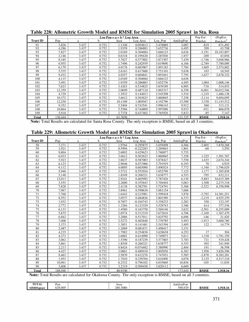
371
Table 228: Allometric Growth Model and RMSE for Simulation 2005 Sprawl in Sta. Rosa
Tract ID Log Pop = a + b * Log Area Pop Est-
PopAct
(PopEst-
PopAct)2 Pop a b Area Log Area Log_Pop AntilogPop
91 3,826 3.437 0.752 1.1340 0.054613 3.478069 3,007 -819 671,492 92 4,286 3.437 0.752 1.9359 0.286883 3.652736 4,495 209 43,708
93 7,827 3.437 0.752 2.0169 0.304684 3.666123 4,636 -3,191 10,183,897
94 2,146 3.437 0.752 0.6318 -0.199420 3.287036 1,937 -209 43,856
95 9,185 3.437 0.752 3.7827 0.577802 3.871507 7,439 -1,746 3,048,966
96 6,955 3.437 0.752 1.7496 0.242939 3.619690 4,166 -2,789 7,780,089
97 6,179 3.437 0.752 4.0176 0.603967 3.891183 7,784 1,605 2,574,882
98 5,535 3.437 0.752 2.6163 0.417688 3.751101 5,638 103 10,545
99 9,432 3.437 0.752 4.0257 0.604841 3.891841 7,795 -1,637 2,678,322
100 4,115 3.437 0.752 2.0169 0.304684 3.666123 4,636
101 3,491 3.437 0.752 1.9359 0.286883 3.652736 4,495 1,004 1,008,146
102 7,623 3.437 0.752 3.4263 0.534825 3.839189 6,905 -718 514,953
103 12,359 3.437 0.752 3.0699 0.487124 3.803317 6,358 -6,001 36,012,546
104 4,729 3.437 0.752 1.3932 0.144013 3.545298 3,510 -1,219 1,486,138
105 10,372 3.437 0.752 3.6612 0.563623 3.860845 7,258 -3,114 9,694,095
106 12,250 3.437 0.752 10.1169 1.005047 4.192796 15,588 3,338 11,143,512
107 9,352 3.437 0.752 5.5404 0.743541 3.996143 9,912 560 313,131
108 10,864 3.437 0.752 5.5566 0.744809 3.997096 9,933 -931 866,078
109 5,918 3.437 0.752 2.7378 0.437402 3.765926 5,833 -85 7,147
Total 136,444 61.3656 121,325 RMSE 1,918.16
Note: Total Results are calculated for Santa Rosa County. The only exception is RMSE, based on all 3 counties.
Table 229: Allometric Growth Model and RMSE for Simulation 2005 Sprawl in Okaloosa
Tract ID Log Pop = a + b * Log Area Pop Est-
PopAct
(PopEst-
PopAct)2 Pop a b Area Log Area Log_Pop AntilogPop
58 7,371 3.437 0.752 1.9764 0.295875 3.659498 4,566 -2,805 7,870,268 59 1,921 3.437 0.752 0.5994 -0.222283 3.269843 1,861 -60 3,550
60 9,804 3.437 0.752 2.6892 0.429623 3.760077 5,755
61 6,033 3.437 0.752 3.6612 0.563623 3.860845 7,258 1,225 1,501,767
62 5,923 3.437 0.752 3.8637 0.587003 3.878427 7,558 1,635 2,674,344
63 6,123 3.437 0.752 2.9646 0.471966 3.791919 6,193 70 4,935
64 9,112 3.437 0.752 4.0095 0.603090 3.890524 7,772 -1,340 1,796,029
65 5,948 3.437 0.752 3.5721 0.552924 3.852799 7,125 1,177 1,385,858
66 5,148 3.437 0.752 1.8549 0.268321 3.638777 4,353 -795 632,211
67 12,013 3.437 0.752 2.9241 0.465992 3.787426 6,130 -5,883 34,615,389
68 3,555 3.437 0.752 2.2680 0.355643 3.704444 5,063 1,508 2,275,318
69 7,828 3.437 0.752 2.4138 0.382701 3.724791 5,306 -2,522 6,358,998
70 7,967 3.437 0.752 3.8961 0.590630 3.881154 7,606
71 7,768 3.437 0.752 1.6443 0.215981 3.599418 3,976 -3,792 14,381,251
72 8,552 3.437 0.752 3.0537 0.484826 3.801589 6,333 -2,219 4,925,259
73 1,932 3.437 0.752 0.7857 -0.104743 3.358233 2,282 350 122,197
74 2,772 3.437 0.752 1.3284 0.123329 3.529743 3,386 614 377,536
75 6,133 3.437 0.752 1.4580 0.163758 3.560146 3,632 -2,501 6,255,009
76 5,875 3.437 0.752 2.0574 0.313319 3.672616 4,706 -1,169 1,367,479
77 6,842 3.437 0.752 3.2886 0.517011 3.825792 6,696 -146 21,420
78 7,406 3.437 0.752 2.5272 0.402640 3.739785 5,493 -1,913 3,660,760
79 3,373 3.437 0.752 1.3851 0.141481 3.543394 3,495 122 14,779
80 2,487 3.437 0.752 1.2069 0.081671 3.498417 3,151
81 4,235 3.437 0.752 1.7982 0.254838 3.628638 4,252 17 304
82 4,273 3.437 0.752 2.6001 0.414990 3.749073 5,611 1,338 1,791,359
83 3,062 3.437 0.752 1.5390 0.187239 3.577803 3,783 721 519,428
84 3,861 3.437 0.752 1.8549 0.268321 3.638777 4,353 492 241,949
85 2,213 3.437 0.752 0.8424 -0.074482 3.380990 2,404 191 36,598
86 4,427 3.437 0.752 3.0861 0.489410 3.805036 6,383 1,956 3,826,596
87 8,463 3.437 0.752 2.5839 0.412276 3.747031 5,585 -2,878 8,282,281
88 1,953 3.437 0.752 1.7010 0.230704 3.610490 4,078 2,125 4,517,318
89 10,961 3.437 0.752 6.2532 0.796102 4.035669 10,856 -105 11,030
90 3,606 3.437 0.752 3.2319 0.509458 3.820112 6,609
Total 188,940 80.9190 173,610 RMSE 1,918.16
Note: Total Results are calculated for Okaloosa County. The only exception is RMSE, based on all 3 counties.
TOTAL Pop
Area
AntilogPop SIM05spraw 629,005 280.3086 590,929 RMSE 1,918.16
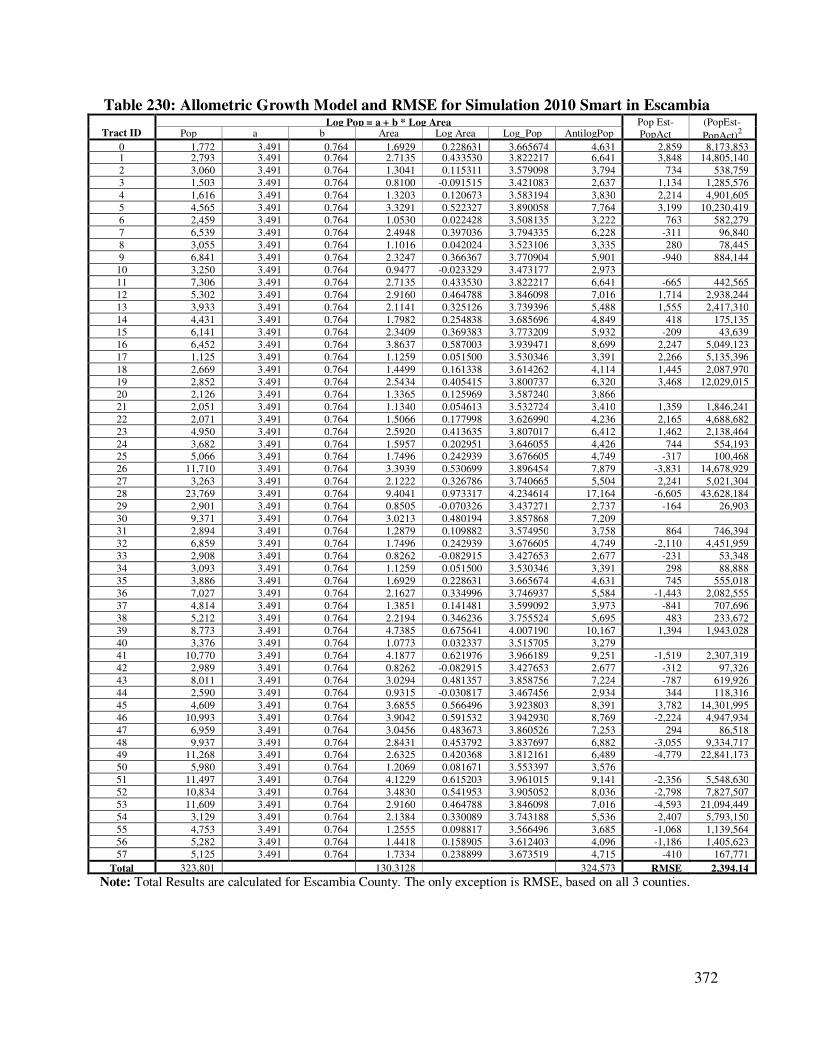
372
Table 230: Allometric Growth Model and RMSE for Simulation 2010 Smart in Escambia
Tract ID Log Pop = a + b * Log Area Pop Est-
PopAct
(PopEst-
PopAct)2 Pop a b Area Log Area Log_Pop AntilogPop
0 1,772 3.491 0.764 1.6929 0.228631 3.665674 4,631 2,859 8,173,853 1 2,793 3.491 0.764 2.7135 0.433530 3.822217 6,641 3,848 14,805,140
2 3,060 3.491 0.764 1.3041 0.115311 3.579098 3,794 734 538,759
3 1,503 3.491 0.764 0.8100 -0.091515 3.421083 2,637 1,134 1,285,576
4 1,616 3.491 0.764 1.3203 0.120673 3.583194 3,830 2,214 4,901,605
5 4,565 3.491 0.764 3.3291 0.522327 3.890058 7,764 3,199 10,230,419
6 2,459 3.491 0.764 1.0530 0.022428 3.508135 3,222 763 582,279
7 6,539 3.491 0.764 2.4948 0.397036 3.794335 6,228 -311 96,840
8 3,055 3.491 0.764 1.1016 0.042024 3.523106 3,335 280 78,445
9 6,841 3.491 0.764 2.3247 0.366367 3.770904 5,901 -940 884,144
10 3,250 3.491 0.764 0.9477 -0.023329 3.473177 2,973
11 7,306 3.491 0.764 2.7135 0.433530 3.822217 6,641 -665 442,565
12 5,302 3.491 0.764 2.9160 0.464788 3.846098 7,016 1,714 2,938,244
13 3,933 3.491 0.764 2.1141 0.325126 3.739396 5,488 1,555 2,417,310
14 4,431 3.491 0.764 1.7982 0.254838 3.685696 4,849 418 175,135
15 6,141 3.491 0.764 2.3409 0.369383 3.773209 5,932 -209 43,639
16 6,452 3.491 0.764 3.8637 0.587003 3.939471 8,699 2,247 5,049,123
17 1,125 3.491 0.764 1.1259 0.051500 3.530346 3,391 2,266 5,135,396
18 2,669 3.491 0.764 1.4499 0.161338 3.614262 4,114 1,445 2,087,970
19 2,852 3.491 0.764 2.5434 0.405415 3.800737 6,320 3,468 12,029,015
20 2,126 3.491 0.764 1.3365 0.125969 3.587240 3,866
21 2,051 3.491 0.764 1.1340 0.054613 3.532724 3,410 1,359 1,846,241
22 2,071 3.491 0.764 1.5066 0.177998 3.626990 4,236 2,165 4,688,682
23 4,950 3.491 0.764 2.5920 0.413635 3.807017 6,412 1,462 2,138,464
24 3,682 3.491 0.764 1.5957 0.202951 3.646055 4,426 744 554,193
25 5,066 3.491 0.764 1.7496 0.242939 3.676605 4,749 -317 100,468
26 11,710 3.491 0.764 3.3939 0.530699 3.896454 7,879 -3,831 14,678,929
27 3,263 3.491 0.764 2.1222 0.326786 3.740665 5,504 2,241 5,021,304
28 23,769 3.491 0.764 9.4041 0.973317 4.234614 17,164 -6,605 43,628,184
29 2,901 3.491 0.764 0.8505 -0.070326 3.437271 2,737 -164 26,903
30 9,371 3.491 0.764 3.0213 0.480194 3.857868 7,209
31 2,894 3.491 0.764 1.2879 0.109882 3.574950 3,758 864 746,394
32 6,859 3.491 0.764 1.7496 0.242939 3.676605 4,749 -2,110 4,451,959
33 2,908 3.491 0.764 0.8262 -0.082915 3.427653 2,677 -231 53,348
34 3,093 3.491 0.764 1.1259 0.051500 3.530346 3,391 298 88,888
35 3,886 3.491 0.764 1.6929 0.228631 3.665674 4,631 745 555,018
36 7,027 3.491 0.764 2.1627 0.334996 3.746937 5,584 -1,443 2,082,555
37 4,814 3.491 0.764 1.3851 0.141481 3.599092 3,973 -841 707,696
38 5,212 3.491 0.764 2.2194 0.346236 3.755524 5,695 483 233,672
39 8,773 3.491 0.764 4.7385 0.675641 4.007190 10,167 1,394 1,943,028
40 3,376 3.491 0.764 1.0773 0.032337 3.515705 3,279
41 10,770 3.491 0.764 4.1877 0.621976 3.966189 9,251 -1,519 2,307,319
42 2,989 3.491 0.764 0.8262 -0.082915 3.427653 2,677 -312 97,326
43 8,011 3.491 0.764 3.0294 0.481357 3.858756 7,224 -787 619,926
44 2,590 3.491 0.764 0.9315 -0.030817 3.467456 2,934 344 118,316
45 4,609 3.491 0.764 3.6855 0.566496 3.923803 8,391 3,782 14,301,995
46 10,993 3.491 0.764 3.9042 0.591532 3.942930 8,769 -2,224 4,947,934
47 6,959 3.491 0.764 3.0456 0.483673 3.860526 7,253 294 86,518
48 9,937 3.491 0.764 2.8431 0.453792 3.837697 6,882 -3,055 9,334,717
49 11,268 3.491 0.764 2.6325 0.420368 3.812161 6,489 -4,779 22,841,173
50 5,980 3.491 0.764 1.2069 0.081671 3.553397 3,576
51 11,497 3.491 0.764 4.1229 0.615203 3.961015 9,141 -2,356 5,548,630
52 10,834 3.491 0.764 3.4830 0.541953 3.905052 8,036 -2,798 7,827,507
53 11,609 3.491 0.764 2.9160 0.464788 3.846098 7,016 -4,593 21,094,449
54 3,129 3.491 0.764 2.1384 0.330089 3.743188 5,536 2,407 5,793,150
55 4,753 3.491 0.764 1.2555 0.098817 3.566496 3,685 -1,068 1,139,564
56 5,282 3.491 0.764 1.4418 0.158905 3.612403 4,096 -1,186 1,405,623
57 5,125 3.491 0.764 1.7334 0.238899 3.673519 4,715 -410 167,771
Total 323,801 130.3128 324,573 RMSE 2,394.14
Note: Total Results are calculated for Escambia County. The only exception is RMSE, based on all 3 counties.

373
Table 231: Allometric Growth Model and RMSE for Simulation 2010 Smart in Santa Rosa
Tract ID Log Pop = a + b * Log Area Pop Est-
PopAct
(PopEst-
PopAct)2 Pop a b Area Log Area Log_Pop AntilogPop
91 4,069 3.491 0.764 1.0206 0.008856 3.497766 3,146 -923 851,836 92 4,463 3.491 0.764 1.6848 0.226548 3.664083 4,614 151 22,818
93 9,305 3.491 0.764 1.7820 0.250908 3.682693 4,816 -4,489 20,150,424
94 2,076 3.491 0.764 0.5427 -0.265440 3.288204 1,942 -134 18,011
95 10,490 3.491 0.764 3.4668 0.539929 3.903506 8,008 -2,482 6,162,015
96 8,020 3.491 0.764 1.6038 0.205150 3.647735 4,444 -3,576 12,790,651
97 6,292 3.491 0.764 3.7422 0.573127 3.928869 8,489 2,197 4,827,882
98 6,275 3.491 0.764 2.3976 0.379777 3.781149 6,042 -233 54,492
99 10,979 3.491 0.764 3.7665 0.575938 3.931017 8,531 -2,448 5,991,101
100 4,730 3.491 0.764 1.9197 0.283233 3.707390 5,098
101 3,895 3.491 0.764 1.8549 0.268321 3.695997 4,966 1,071 1,146,800
102 8,645 3.491 0.764 3.1590 0.499550 3.872656 7,459 -1,186 1,407,602
103 15,155 3.491 0.764 2.8026 0.447561 3.832937 6,807 -8,348 69,694,091
104 6,045 3.491 0.764 1.3932 0.144013 3.601026 3,990 -2,055 4,221,009
105 12,363 3.491 0.764 3.4182 0.533797 3.898821 7,922 -4,441 19,724,680
106 15,471 3.491 0.764 9.4608 0.975928 4.236609 17,243 1,772 3,139,429
107 11,660 3.491 0.764 5.2731 0.722066 4.042658 11,032 -628 394,251
108 13,310 3.491 0.764 5.1273 0.709889 4.033355 10,798 -2,512 6,308,687
109 6,208 3.491 0.764 2.5596 0.408172 3.802843 6,351 143 20,455
Total 159,451 56.9754 131,697 RMSE 2,394.14
Note: Total Results are calculated for Santa Rosa County. The only exception is RMSE, based on all 3 counties.
Table 232: Allometric Growth Model and RMSE for Simulation 2010 Smart in Okaloosa
Tract ID Log Pop = a + b * Log Area Pop Est-
PopAct
(PopEst-
PopAct)2 Pop a b Area Log Area Log_Pop AntilogPop
58 7,983 3.491 0.764 1.7253 0.236865 3.671965 4,699 -3,284 10,787,561 59 2,032 3.491 0.764 0.5508 -0.259006 3.293119 1,964 -68 4,638
60 11,212 3.491 0.764 2.3571 0.372378 3.775497 5,963
61 6,521 3.491 0.764 3.4344 0.535851 3.900390 7,950 1,429 2,043,241
62 6,352 3.491 0.764 3.5802 0.553907 3.914185 8,207 1,855 3,441,077
63 6,923 3.491 0.764 2.8107 0.448814 3.833894 6,822 -101 10,256
64 10,600 3.491 0.764 3.7746 0.576871 3.931729 8,545 -2,055 4,221,624
65 6,518 3.491 0.764 3.5235 0.546974 3.908888 8,108 1,590 2,526,593
66 5,740 3.491 0.764 1.7901 0.252877 3.684198 4,833 -907 823,023
67 14,795 3.491 0.764 2.6973 0.430929 3.820230 6,610 -8,185 66,987,127
68 3,786 3.491 0.764 2.1870 0.339849 3.750644 5,632 1,846 3,406,846
69 8,361 3.491 0.764 2.2518 0.352530 3.760333 5,759 -2,602 6,771,391
70 8,392 3.491 0.764 3.6855 0.566496 3.923803 8,391
71 8,160 3.491 0.764 1.5876 0.200741 3.644366 4,409 -3,751 14,068,014
72 9,152 3.491 0.764 2.8998 0.462368 3.844249 6,986 -2,166 4,690,120
73 2,006 3.491 0.764 0.7128 -0.147032 3.378667 2,391 385 148,597
74 2,873 3.491 0.764 1.2393 0.093176 3.562187 3,649 776 602,345
75 7,031 3.491 0.764 1.4499 0.161338 3.614262 4,114 -2,917 8,509,000
76 6,685 3.491 0.764 1.9521 0.290502 3.712944 5,163 -1,522 2,314,984
77 7,356 3.491 0.764 3.0375 0.482516 3.859642 7,238 -118 13,830
78 7,755 3.491 0.764 2.4138 0.382701 3.783384 6,073 -1,682 2,830,041
79 3,510 3.491 0.764 1.3365 0.125969 3.587240 3,866 356 126,599
80 2,619 3.491 0.764 1.1259 0.051500 3.530346 3,391
81 4,394 3.491 0.764 1.7172 0.234821 3.670403 4,682 288 82,769
82 4,425 3.491 0.764 2.5029 0.398443 3.795411 6,243 1,818 3,306,039
83 3,232 3.491 0.764 1.5147 0.180327 3.628770 4,254 1,022 1,043,925
84 3,998 3.491 0.764 1.7820 0.250908 3.682693 4,816 818 669,251
85 2,378 3.491 0.764 0.8262 -0.082915 3.427653 2,677 299 89,418
86 4,664 3.491 0.764 2.9727 0.473151 3.852487 7,120 2,456 6,032,535
87 9,544 3.491 0.764 2.4705 0.392785 3.791088 6,181 -3,363 11,307,004
88 2,070 3.491 0.764 1.5957 0.202951 3.646055 4,426 2,356 5,552,818
89 12,810 3.491 0.764 5.8401 0.766420 4.076545 11,927 -883 779,016
90 4,032 3.491 0.764 3.0861 0.489410 3.864909 7,327
Total 207,909 76.4316 190,418 RMSE 2,394.14
Note: Total Results are calculated for Okaloosa County. The only exception is RMSE, based on all 3 counties.
TOTAL Pop
Area
AntilogPop SIM10smart 691,161 263.7198 646,688 RMSE 2,394.14
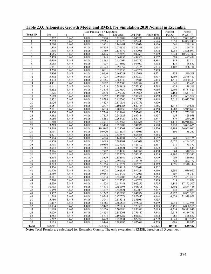
374
Table 233: Allometric Growth Model and RMSE for Simulation 2010 Normal in Escambia
Tract ID Log Pop = a + b * Log Area Pop Est-
PopAct
(PopEst-
PopAct)2 Pop a b Area Log Area Log_Pop AntilogPop
0 1,772 3.443 0.806 1.7820 0.250908 3.645232 4,418 2,646 7,001,633 1 2,793 3.443 0.806 2.9565 0.470778 3.822447 6,644 3,851 14,832,245
2 3,060 3.443 0.806 1.3851 0.141481 3.557034 3,606 546 298,189
3 1,503 3.443 0.806 0.8505 -0.070326 3.386318 2,434 931 866,729
4 1,616 3.443 0.806 1.3689 0.136372 3.552916 3,572 1,956 3,826,070
5 4,565 3.443 0.806 3.6126 0.557820 3.892603 7,809 3,244 10,524,399
6 2,459 3.443 0.806 1.1745 0.069853 3.499302 3,157 698 487,478
7 6,539 3.443 0.806 2.8188 0.450064 3.805752 6,394 -145 21,114
8 3,055 3.443 0.806 1.1907 0.075802 3.504097 3,192 137 18,837
9 6,841 3.443 0.806 2.4624 0.391359 3.758435 5,734 -1,107 1,226,111
10 3,250 3.443 0.806 1.0611 0.025756 3.463760 2,909
11 7,306 3.443 0.806 2.9160 0.464788 3.817619 6,571 -735 540,508
12 5,302 3.443 0.806 3.1023 0.491684 3.839297 6,907 1,605 2,576,417
13 3,933 3.443 0.806 2.3085 0.363330 3.735844 5,443 1,510 2,280,310
14 4,431 3.443 0.806 1.9602 0.292300 3.678594 4,771 340 115,486
15 6,141 3.443 0.806 2.4543 0.389928 3.757282 5,718 -423 178,511
16 6,452 3.443 0.806 4.3416 0.637650 3.956946 9,056 2,604 6,781,829
17 1,125 3.443 0.806 1.2312 0.090329 3.515805 3,279 2,154 4,641,780
18 2,669 3.443 0.806 1.5552 0.191786 3.597580 3,959 1,290 1,663,964
19 2,852 3.443 0.806 2.8593 0.456260 3.810745 6,468 3,616 13,072,799
20 2,126 3.443 0.806 1.4823 0.170936 3.580775 3,809
21 2,051 3.443 0.806 1.2717 0.104385 3.527134 3,366 1,315 1,729,631
22 2,071 3.443 0.806 1.6038 0.205150 3.608351 4,058 1,987 3,949,618
23 4,950 3.443 0.806 2.7540 0.439964 3.797611 6,275 1,325 1,755,518
24 3,682 3.443 0.806 1.7415 0.240923 3.637184 4,337 655 428,958
25 5,066 3.443 0.806 1.8468 0.266420 3.657734 4,547 -519 269,258
26 11,710 3.443 0.806 3.4911 0.542962 3.880628 7,597 -4,113 16,918,859
27 3,263 3.443 0.806 2.3490 0.370883 3.741932 5,520 2,257 5,093,626
28 23,769 3.443 0.806 10.5867 1.024761 4.268957 18,576 -5,193 26,965,096
29 2,901 3.443 0.806 0.9720 -0.012334 3.433059 2,711 -190 36,267
30 9,371 3.443 0.806 3.3696 0.527578 3.868228 7,383
31 2,894 3.443 0.806 1.4094 0.149034 3.563122 3,657 763 582,126
32 6,859 3.443 0.806 1.9683 0.294091 3.680038 4,787 -2,072 4,294,365
33 2,908 3.443 0.806 0.9396 -0.027057 3.421192 2,637 -271 73,172
34 3,093 3.443 0.806 1.1583 0.063821 3.494440 3,122 29 844
35 3,886 3.443 0.806 1.7982 0.254838 3.648399 4,450 564 318,552
36 7,027 3.443 0.806 2.3571 0.372378 3.743137 5,535 -1,492 2,225,340
37 4,814 3.443 0.806 1.5309 0.184947 3.592067 3,909 -905 819,001
38 5,212 3.443 0.806 2.4624 0.391359 3.758435 5,734 522 272,172
39 8,773 3.443 0.806 5.1354 0.710574 4.015723 10,369 1,596 2,546,149
40 3,376 3.443 0.806 1.2555 0.098817 3.522646 3,332
41 10,770 3.443 0.806 4.6008 0.662833 3.977244 9,490 -1,280 1,639,660
42 2,989 3.443 0.806 0.9153 -0.038437 3.412020 2,582 -407 165,340
43 8,011 3.443 0.806 3.3534 0.525485 3.866541 7,354 -657 431,258
44 2,590 3.443 0.806 1.0611 0.025756 3.463760 2,909 319 101,829
45 4,609 3.443 0.806 4.1634 0.619448 3.942275 8,755 4,146 17,192,500
46 10,993 3.443 0.806 4.4874 0.651995 3.968508 9,301 -1,692 2,864,448
47 6,959 3.443 0.806 3.3777 0.528621 3.869069 7,397 438 192,038
48 9,937 3.443 0.806 3.1347 0.496196 3.842934 6,965 -2,972 8,831,560
49 11,268 3.443 0.806 2.9565 0.470778 3.822447 6,644 -4,624 21,378,921
50 5,980 3.443 0.806 1.3041 0.115311 3.535941 3,435
51 11,497 3.443 0.806 4.5765 0.660533 3.975390 9,449 -2,048 4,193,936
52 10,834 3.443 0.806 3.9447 0.596014 3.923387 8,383 -2,451 6,008,555
53 11,609 3.443 0.806 3.2076 0.506180 3.850981 7,095 -4,514 20,371,942
54 3,129 3.443 0.806 2.4138 0.382701 3.751457 5,642 2,513 6,316,746
55 4,753 3.443 0.806 1.5714 0.196287 3.601207 3,992 -761 578,889
56 5,282 3.443 0.806 1.6929 0.228631 3.627277 4,239 -1,043 1,087,576
57 5,125 3.443 0.806 1.9440 0.288696 3.675689 4,739 -386 148,975
Total 323,801 143.5806 326,125 RMSE 2,287.02
Note: Total Results are calculated for Escambia County. The only exception is RMSE, based on all 3 counties.
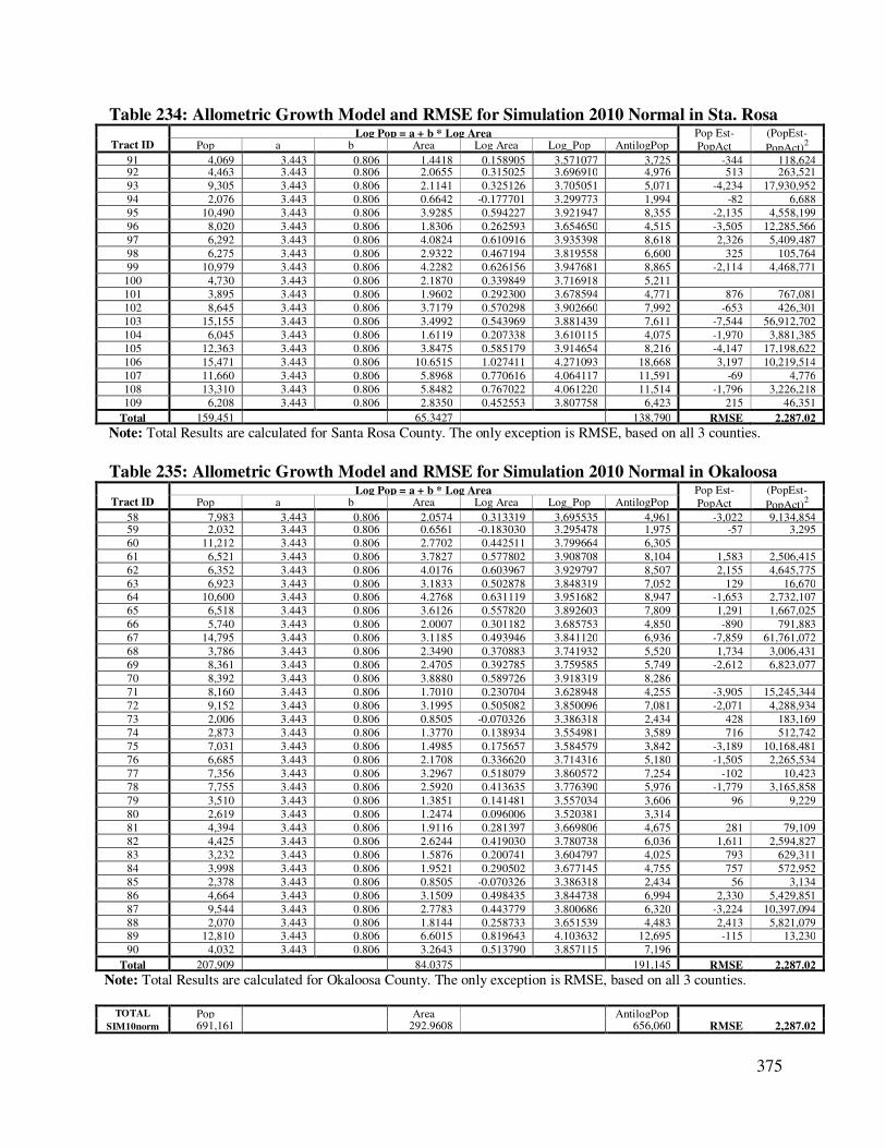
375
Table 234: Allometric Growth Model and RMSE for Simulation 2010 Normal in Sta. Rosa
Tract ID Log Pop = a + b * Log Area Pop Est-
PopAct
(PopEst-
PopAct)2 Pop a b Area Log Area Log_Pop AntilogPop
91 4,069 3.443 0.806 1.4418 0.158905 3.571077 3,725 -344 118,624 92 4,463 3.443 0.806 2.0655 0.315025 3.696910 4,976 513 263,521
93 9,305 3.443 0.806 2.1141 0.325126 3.705051 5,071 -4,234 17,930,952
94 2,076 3.443 0.806 0.6642 -0.177701 3.299773 1,994 -82 6,688
95 10,490 3.443 0.806 3.9285 0.594227 3.921947 8,355 -2,135 4,558,199
96 8,020 3.443 0.806 1.8306 0.262593 3.654650 4,515 -3,505 12,285,566
97 6,292 3.443 0.806 4.0824 0.610916 3.935398 8,618 2,326 5,409,487
98 6,275 3.443 0.806 2.9322 0.467194 3.819558 6,600 325 105,764
99 10,979 3.443 0.806 4.2282 0.626156 3.947681 8,865 -2,114 4,468,771
100 4,730 3.443 0.806 2.1870 0.339849 3.716918 5,211
101 3,895 3.443 0.806 1.9602 0.292300 3.678594 4,771 876 767,081
102 8,645 3.443 0.806 3.7179 0.570298 3.902660 7,992 -653 426,301
103 15,155 3.443 0.806 3.4992 0.543969 3.881439 7,611 -7,544 56,912,702
104 6,045 3.443 0.806 1.6119 0.207338 3.610115 4,075 -1,970 3,881,385
105 12,363 3.443 0.806 3.8475 0.585179 3.914654 8,216 -4,147 17,198,622
106 15,471 3.443 0.806 10.6515 1.027411 4.271093 18,668 3,197 10,219,514
107 11,660 3.443 0.806 5.8968 0.770616 4.064117 11,591 -69 4,776
108 13,310 3.443 0.806 5.8482 0.767022 4.061220 11,514 -1,796 3,226,218
109 6,208 3.443 0.806 2.8350 0.452553 3.807758 6,423 215 46,351
Total 159,451 65.3427 138,790 RMSE 2,287.02
Note: Total Results are calculated for Santa Rosa County. The only exception is RMSE, based on all 3 counties.
Table 235: Allometric Growth Model and RMSE for Simulation 2010 Normal in Okaloosa
Tract ID Log Pop = a + b * Log Area Pop Est-
PopAct
(PopEst-
PopAct)2 Pop a b Area Log Area Log_Pop AntilogPop
58 7,983 3.443 0.806 2.0574 0.313319 3.695535 4,961 -3,022 9,134,854 59 2,032 3.443 0.806 0.6561 -0.183030 3.295478 1,975 -57 3,295
60 11,212 3.443 0.806 2.7702 0.442511 3.799664 6,305
61 6,521 3.443 0.806 3.7827 0.577802 3.908708 8,104 1,583 2,506,415
62 6,352 3.443 0.806 4.0176 0.603967 3.929797 8,507 2,155 4,645,775
63 6,923 3.443 0.806 3.1833 0.502878 3.848319 7,052 129 16,670
64 10,600 3.443 0.806 4.2768 0.631119 3.951682 8,947 -1,653 2,732,107
65 6,518 3.443 0.806 3.6126 0.557820 3.892603 7,809 1,291 1,667,025
66 5,740 3.443 0.806 2.0007 0.301182 3.685753 4,850 -890 791,883
67 14,795 3.443 0.806 3.1185 0.493946 3.841120 6,936 -7,859 61,761,072
68 3,786 3.443 0.806 2.3490 0.370883 3.741932 5,520 1,734 3,006,431
69 8,361 3.443 0.806 2.4705 0.392785 3.759585 5,749 -2,612 6,823,077
70 8,392 3.443 0.806 3.8880 0.589726 3.918319 8,286
71 8,160 3.443 0.806 1.7010 0.230704 3.628948 4,255 -3,905 15,245,344
72 9,152 3.443 0.806 3.1995 0.505082 3.850096 7,081 -2,071 4,288,934
73 2,006 3.443 0.806 0.8505 -0.070326 3.386318 2,434 428 183,169
74 2,873 3.443 0.806 1.3770 0.138934 3.554981 3,589 716 512,742
75 7,031 3.443 0.806 1.4985 0.175657 3.584579 3,842 -3,189 10,168,481
76 6,685 3.443 0.806 2.1708 0.336620 3.714316 5,180 -1,505 2,265,534
77 7,356 3.443 0.806 3.2967 0.518079 3.860572 7,254 -102 10,423
78 7,755 3.443 0.806 2.5920 0.413635 3.776390 5,976 -1,779 3,165,858
79 3,510 3.443 0.806 1.3851 0.141481 3.557034 3,606 96 9,229
80 2,619 3.443 0.806 1.2474 0.096006 3.520381 3,314
81 4,394 3.443 0.806 1.9116 0.281397 3.669806 4,675 281 79,109
82 4,425 3.443 0.806 2.6244 0.419030 3.780738 6,036 1,611 2,594,827
83 3,232 3.443 0.806 1.5876 0.200741 3.604797 4,025 793 629,311
84 3,998 3.443 0.806 1.9521 0.290502 3.677145 4,755 757 572,952
85 2,378 3.443 0.806 0.8505 -0.070326 3.386318 2,434 56 3,134
86 4,664 3.443 0.806 3.1509 0.498435 3.844738 6,994 2,330 5,429,851
87 9,544 3.443 0.806 2.7783 0.443779 3.800686 6,320 -3,224 10,397,094
88 2,070 3.443 0.806 1.8144 0.258733 3.651539 4,483 2,413 5,821,079
89 12,810 3.443 0.806 6.6015 0.819643 4.103632 12,695 -115 13,230
90 4,032 3.443 0.806 3.2643 0.513790 3.857115 7,196
Total 207,909 84.0375 191,145 RMSE 2,287.02
Note: Total Results are calculated for Okaloosa County. The only exception is RMSE, based on all 3 counties.
TOTAL Pop
Area
AntilogPop SIM10norm 691,161 292.9608 656,060 RMSE 2,287.02

376
Table 236: Allometric Growth Model and RMSE for Simulation 2010 Sprawl in Escambia
Tract ID Log Pop = a + b * Log Area Pop Est-
PopAct
(PopEst-
PopAct)2 Pop a b Area Log Area Log_Pop AntilogPop
0 1,772 3.418 0.813 1.8063 0.256790 3.626770 4,234 2,462 6,062,372 1 2,793 3.418 0.813 3.0699 0.487124 3.814032 6,517 3,724 13,866,419
2 3,060 3.418 0.813 1.4175 0.151523 3.541188 3,477 417 173,779
3 1,503 3.418 0.813 0.9072 -0.042297 3.383613 2,419 916 838,818
4 1,616 3.418 0.813 1.4499 0.161338 3.549168 3,541 1,925 3,706,941
5 4,565 3.418 0.813 3.8556 0.586092 3.894493 7,843 3,278 10,746,534
6 2,459 3.418 0.813 1.2474 0.096006 3.496053 3,134 675 455,174
7 6,539 3.418 0.813 2.9889 0.475511 3.804591 6,377 -162 26,366
8 3,055 3.418 0.813 1.2150 0.084576 3.486761 3,067 12 152
9 6,841 3.418 0.813 2.6406 0.421703 3.760844 5,766 -1,075 1,156,493
10 3,250 3.418 0.813 1.1502 0.060773 3.467409 2,934
11 7,306 3.418 0.813 3.1590 0.499550 3.824134 6,670 -636 404,339
12 5,302 3.418 0.813 3.2238 0.508368 3.831303 6,781 1,479 2,187,880
13 3,933 3.418 0.813 2.4786 0.394206 3.738490 5,476 1,543 2,381,876
14 4,431 3.418 0.813 2.1303 0.328441 3.685022 4,842 411 168,899
15 6,141 3.418 0.813 2.5434 0.405415 3.747602 5,592 -549 300,907
16 6,452 3.418 0.813 4.7385 0.675641 3.967296 9,275 2,823 7,967,173
17 1,125 3.418 0.813 1.2393 0.093176 3.493752 3,117 1,992 3,968,512
18 2,669 3.418 0.813 1.5309 0.184947 3.568362 3,701 1,032 1,065,775
19 2,852 3.418 0.813 2.9646 0.471966 3.801708 6,334 3,482 12,127,410
20 2,126 3.418 0.813 1.5390 0.187239 3.570225 3,717
21 2,051 3.418 0.813 1.3122 0.118000 3.513934 3,265 1,214 1,474,724
22 2,071 3.418 0.813 1.7091 0.232767 3.607240 4,048 1,977 3,908,509
23 4,950 3.418 0.813 2.9241 0.465992 3.796852 6,264 1,314 1,726,593
24 3,682 3.418 0.813 1.8711 0.272097 3.639215 4,357 675 455,995
25 5,066 3.418 0.813 2.0817 0.318418 3.676874 4,752 -314 98,613
26 11,710 3.418 0.813 3.5235 0.546974 3.862690 7,289 -4,421 19,541,956
27 3,263 3.418 0.813 2.4786 0.394206 3.738490 5,476 2,213 4,898,843
28 23,769 3.418 0.813 11.3238 1.053992 4.274896 18,832 -4,937 24,374,309
29 2,901 3.418 0.813 1.0206 0.008856 3.425200 2,662 -239 57,146
30 9,371 3.418 0.813 3.6450 0.561698 3.874660 7,493
31 2,894 3.418 0.813 1.4985 0.175657 3.560809 3,638 744 552,866
32 6,859 3.418 0.813 1.9683 0.294091 3.657096 4,540 -2,319 5,375,804
33 2,908 3.418 0.813 0.9558 -0.019633 3.402038 2,524 -384 147,684
34 3,093 3.418 0.813 1.1664 0.066848 3.472347 2,967 -126 15,825
35 3,886 3.418 0.813 1.9521 0.290502 3.654178 4,510 624 389,397
36 7,027 3.418 0.813 2.5596 0.408172 3.749844 5,621 -1,406 1,975,732
37 4,814 3.418 0.813 1.5228 0.182643 3.566489 3,685 -1,129 1,273,661
38 5,212 3.418 0.813 2.5677 0.409544 3.750960 5,636 424 179,650
39 8,773 3.418 0.813 5.5809 0.746704 4.025071 10,594 1,821 3,316,981
40 3,376 3.418 0.813 1.2717 0.104385 3.502865 3,183
41 10,770 3.418 0.813 4.9653 0.695945 3.983804 9,634 -1,136 1,290,645
42 2,989 3.418 0.813 0.9396 -0.027057 3.396003 2,489 -500 250,127
43 8,011 3.418 0.813 3.5235 0.546974 3.862690 7,289 -722 520,748
44 2,590 3.418 0.813 1.1016 0.042024 3.452165 2,832 242 58,792
45 4,609 3.418 0.813 4.3416 0.637650 3.936409 8,638 4,029 16,232,215
46 10,993 3.418 0.813 4.8195 0.683002 3.973281 9,403 -1,590 2,527,124
47 6,959 3.418 0.813 3.6693 0.564583 3.877006 7,534 575 330,237
48 9,937 3.418 0.813 3.3291 0.522327 3.842652 6,961 -2,976 8,858,476
49 11,268 3.418 0.813 3.2319 0.509458 3.832189 6,795 -4,473 20,007,754
50 5,980 3.418 0.813 1.3851 0.141481 3.533024 3,412
51 11,497 3.418 0.813 4.9734 0.696653 3.984379 9,647 -1,850 3,423,574
52 10,834 3.418 0.813 4.4226 0.645678 3.942936 8,769 -2,065 4,265,403
53 11,609 3.418 0.813 3.4344 0.535851 3.853647 7,139 -4,470 19,979,522
54 3,129 3.418 0.813 2.6163 0.417688 3.757580 5,722 2,593 6,725,844
55 4,753 3.418 0.813 1.8549 0.268321 3.636145 4,327 -426 181,835
56 5,282 3.418 0.813 1.9359 0.286883 3.651236 4,480 -802 643,902
57 5,125 3.418 0.813 2.1708 0.336620 3.691672 4,917 -208 43,397
Total 323,801 152.9442 326,140 RMSE 2,257.32
Note: Total Results are calculated for Escambia County. The only exception is RMSE, based on all 3 counties.
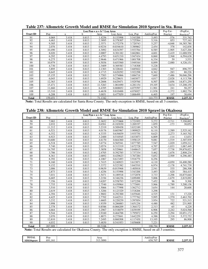
377
Table 237: Allometric Growth Model and RMSE for Simulation 2010 Sprawl in Sta. Rosa
Tract ID Log Pop = a + b * Log Area Pop Est-
PopAct
(PopEst-
PopAct)2 Pop a b Area Log Area Log_Pop AntilogPop
91 4,069 3.418 0.813 1.4256 0.153998 3.543200 3,493 -576 331,762 92 4,463 3.418 0.813 2.3895 0.378307 3.725564 5,316 853 727,163
93 9,305 3.418 0.813 2.3571 0.372378 3.720743 5,257 -4,048 16,385,780
94 2,076 3.418 0.813 0.9234 -0.034610 3.389862 2,454 378 142,830
95 10,490 3.418 0.813 4.3092 0.634397 3.933764 8,585 -1,905 3,627,204
96 8,020 3.418 0.813 2.0007 0.301182 3.662861 4,601 -3,419 11,688,930
97 6,292 3.418 0.813 4.4793 0.651210 3.947434 8,860 2,568 6,594,638
98 6,275 3.418 0.813 2.9646 0.471966 3.801708 6,334 59 3,533
99 10,979 3.418 0.813 4.5036 0.653560 3.949344 8,899 -2,080 4,326,151
100 4,730 3.418 0.813 2.3409 0.369383 3.718308 5,228
101 3,895 3.418 0.813 2.1303 0.328441 3.685022 4,842 947 896,757
102 8,645 3.418 0.813 4.1715 0.620292 3.922298 8,362 -283 80,226
103 15,155 3.418 0.813 3.7503 0.574066 3.884716 7,669 -7,486 56,046,296
104 6,045 3.418 0.813 1.6929 0.228631 3.603877 4,017 -2,028 4,113,706
105 12,363 3.418 0.813 4.2606 0.629471 3.929760 8,507 -3,856 14,871,259
106 15,471 3.418 0.813 11.5263 1.061690 4.281154 19,105 3,634 13,208,150
107 11,660 3.418 0.813 6.4395 0.808852 4.075597 11,901 241 58,257
108 13,310 3.418 0.813 6.4638 0.810488 4.076927 11,938 -1,372 1,882,754
109 6,208 3.418 0.813 3.0051 0.477859 3.806499 6,405 197 38,694
Total 159,451 71.1342 141,773 RMSE 2,257.32
Note: Total Results are calculated for Santa Rosa County. The only exception is RMSE, based on all 3 counties.
Table 238: Allometric Growth Model and RMSE for Simulation 2010 Sprawl in Okaloosa
Tract ID Log Pop = a + b * Log Area Pop Est-
PopAct
(PopEst-
PopAct)2 Pop a b Area Log Area Log_Pop AntilogPop
58 7,983 3.418 0.813 2.3652 0.373868 3.721955 5,272 -2,711 7,350,892 59 2,032 3.418 0.813 0.6561 -0.183030 3.269197 1,859 -173 30,052
60 11,212 3.418 0.813 3.2319 0.509458 3.832189 6,795
61 6,521 3.418 0.813 4.0176 0.603967 3.909025 8,110 1,589 2,525,162
62 6,352 3.418 0.813 4.3335 0.636839 3.935750 8,625 2,273 5,165,702
63 6,923 3.418 0.813 3.2400 0.510545 3.833073 6,809 -114 13,033
64 10,600 3.418 0.813 4.6170 0.664360 3.958125 9,081 -1,519 2,307,939
65 6,518 3.418 0.813 3.6774 0.565541 3.877785 7,547 1,029 1,059,212
66 5,740 3.418 0.813 2.0574 0.313319 3.672728 4,707 -1,033 1,067,449
67 14,795 3.418 0.813 3.3858 0.529661 3.848615 7,057 -7,738 59,878,022
68 3,786 3.418 0.813 2.4705 0.392785 3.737334 5,462 1,676 2,808,234
69 8,361 3.418 0.813 2.6892 0.429623 3.767284 5,852 -2,509 6,296,483
70 8,392 3.418 0.813 4.1067 0.613493 3.916770 8,256
71 8,160 3.418 0.813 1.7415 0.240923 3.613871 4,110 -4,050 16,400,280
72 9,152 3.418 0.813 3.3372 0.523382 3.843510 6,974 -2,178 4,741,739
73 2,006 3.418 0.813 0.9639 -0.015968 3.405018 2,541 535 286,308
74 2,873 3.418 0.813 1.4256 0.153998 3.543200 3,493 620 384,415
75 7,031 3.418 0.813 1.5471 0.189518 3.572078 3,733 -3,298 10,875,644
76 6,685 3.418 0.813 2.2194 0.346236 3.699490 5,006 -1,679 2,819,092
77 7,356 3.418 0.813 3.6207 0.558793 3.872298 7,452 96 9,300
78 7,755 3.418 0.813 2.7540 0.439964 3.775691 5,966 -1,789 3,200,156
79 3,510 3.418 0.813 1.5066 0.177998 3.562712 3,654 144 20,600
80 2,619 3.418 0.813 1.3284 0.123329 3.518266 3,298
81 4,394 3.418 0.813 1.9602 0.292300 3.655640 4,525 131 17,220
82 4,425 3.418 0.813 2.7702 0.442511 3.777762 5,995 1,570 2,463,702
83 3,232 3.418 0.813 1.6605 0.220239 3.597054 3,954 722 521,515
84 3,998 3.418 0.813 1.9359 0.286883 3.651236 4,480 482 231,905
85 2,378 3.418 0.813 0.8586 -0.066209 3.364172 2,313 -65 4,228
86 4,664 3.418 0.813 3.2967 0.518079 3.839199 6,906 2,242 5,024,568
87 9,544 3.418 0.813 2.9160 0.464788 3.795872 6,250 -3,294 10,851,172
88 2,070 3.418 0.813 1.8873 0.275841 3.642259 4,388 2,318 5,372,752
89 12,810 3.418 0.813 7.2495 0.860308 4.117430 13,105 295 86,908
90 4,032 3.418 0.813 3.4830 0.541953 3.858608 7,221
Total 207,909 89.3106 190,794 RMSE 2,257.32
Note: Total Results are calculated for Okaloosa County. The only exception is RMSE, based on all 3 counties.
TOTAL Pop
Area
AntilogPop SIM10spraw 691,161 313.3890 658,707 RMSE 2,257.32
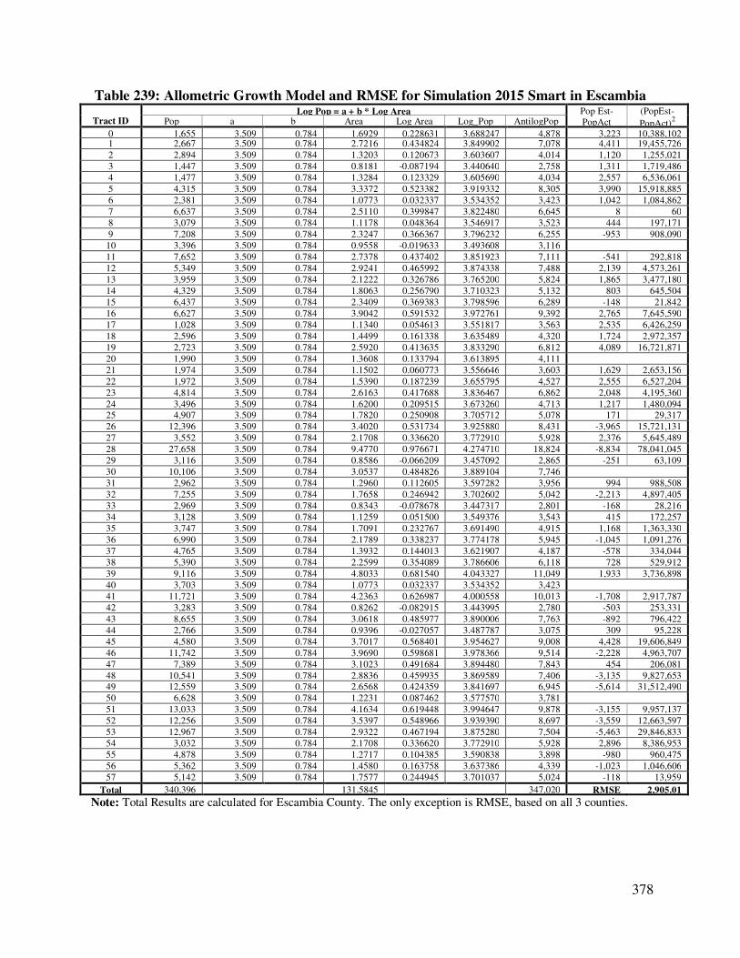
378
Table 239: Allometric Growth Model and RMSE for Simulation 2015 Smart in Escambia
Tract ID Log Pop = a + b * Log Area Pop Est-
PopAct
(PopEst-
PopAct)2 Pop a b Area Log Area Log_Pop AntilogPop
0 1,655 3.509 0.784 1.6929 0.228631 3.688247 4,878 3,223 10,388,102 1 2,667 3.509 0.784 2.7216 0.434824 3.849902 7,078 4,411 19,455,726
2 2,894 3.509 0.784 1.3203 0.120673 3.603607 4,014 1,120 1,255,021
3 1,447 3.509 0.784 0.8181 -0.087194 3.440640 2,758 1,311 1,719,486
4 1,477 3.509 0.784 1.3284 0.123329 3.605690 4,034 2,557 6,536,061
5 4,315 3.509 0.784 3.3372 0.523382 3.919332 8,305 3,990 15,918,885
6 2,381 3.509 0.784 1.0773 0.032337 3.534352 3,423 1,042 1,084,862
7 6,637 3.509 0.784 2.5110 0.399847 3.822480 6,645 8 60
8 3,079 3.509 0.784 1.1178 0.048364 3.546917 3,523 444 197,171
9 7,208 3.509 0.784 2.3247 0.366367 3.796232 6,255 -953 908,090
10 3,396 3.509 0.784 0.9558 -0.019633 3.493608 3,116
11 7,652 3.509 0.784 2.7378 0.437402 3.851923 7,111 -541 292,818
12 5,349 3.509 0.784 2.9241 0.465992 3.874338 7,488 2,139 4,573,261
13 3,959 3.509 0.784 2.1222 0.326786 3.765200 5,824 1,865 3,477,180
14 4,329 3.509 0.784 1.8063 0.256790 3.710323 5,132 803 645,504
15 6,437 3.509 0.784 2.3409 0.369383 3.798596 6,289 -148 21,842
16 6,627 3.509 0.784 3.9042 0.591532 3.972761 9,392 2,765 7,645,590
17 1,028 3.509 0.784 1.1340 0.054613 3.551817 3,563 2,535 6,426,259
18 2,596 3.509 0.784 1.4499 0.161338 3.635489 4,320 1,724 2,972,357
19 2,723 3.509 0.784 2.5920 0.413635 3.833290 6,812 4,089 16,721,871
20 1,990 3.509 0.784 1.3608 0.133794 3.613895 4,111
21 1,974 3.509 0.784 1.1502 0.060773 3.556646 3,603 1,629 2,653,156
22 1,972 3.509 0.784 1.5390 0.187239 3.655795 4,527 2,555 6,527,204
23 4,814 3.509 0.784 2.6163 0.417688 3.836467 6,862 2,048 4,195,360
24 3,496 3.509 0.784 1.6200 0.209515 3.673260 4,713 1,217 1,480,094
25 4,907 3.509 0.784 1.7820 0.250908 3.705712 5,078 171 29,317
26 12,396 3.509 0.784 3.4020 0.531734 3.925880 8,431 -3,965 15,721,131
27 3,552 3.509 0.784 2.1708 0.336620 3.772910 5,928 2,376 5,645,489
28 27,658 3.509 0.784 9.4770 0.976671 4.274710 18,824 -8,834 78,041,045
29 3,116 3.509 0.784 0.8586 -0.066209 3.457092 2,865 -251 63,109
30 10,106 3.509 0.784 3.0537 0.484826 3.889104 7,746
31 2,962 3.509 0.784 1.2960 0.112605 3.597282 3,956 994 988,508
32 7,255 3.509 0.784 1.7658 0.246942 3.702602 5,042 -2,213 4,897,405
33 2,969 3.509 0.784 0.8343 -0.078678 3.447317 2,801 -168 28,216
34 3,128 3.509 0.784 1.1259 0.051500 3.549376 3,543 415 172,257
35 3,747 3.509 0.784 1.7091 0.232767 3.691490 4,915 1,168 1,363,330
36 6,990 3.509 0.784 2.1789 0.338237 3.774178 5,945 -1,045 1,091,276
37 4,765 3.509 0.784 1.3932 0.144013 3.621907 4,187 -578 334,044
38 5,390 3.509 0.784 2.2599 0.354089 3.786606 6,118 728 529,912
39 9,116 3.509 0.784 4.8033 0.681540 4.043327 11,049 1,933 3,736,898
40 3,703 3.509 0.784 1.0773 0.032337 3.534352 3,423
41 11,721 3.509 0.784 4.2363 0.626987 4.000558 10,013 -1,708 2,917,787
42 3,283 3.509 0.784 0.8262 -0.082915 3.443995 2,780 -503 253,331
43 8,655 3.509 0.784 3.0618 0.485977 3.890006 7,763 -892 796,422
44 2,766 3.509 0.784 0.9396 -0.027057 3.487787 3,075 309 95,228
45 4,580 3.509 0.784 3.7017 0.568401 3.954627 9,008 4,428 19,606,849
46 11,742 3.509 0.784 3.9690 0.598681 3.978366 9,514 -2,228 4,963,707
47 7,389 3.509 0.784 3.1023 0.491684 3.894480 7,843 454 206,081
48 10,541 3.509 0.784 2.8836 0.459935 3.869589 7,406 -3,135 9,827,653
49 12,559 3.509 0.784 2.6568 0.424359 3.841697 6,945 -5,614 31,512,490
50 6,628 3.509 0.784 1.2231 0.087462 3.577570 3,781
51 13,033 3.509 0.784 4.1634 0.619448 3.994647 9,878 -3,155 9,957,137
52 12,256 3.509 0.784 3.5397 0.548966 3.939390 8,697 -3,559 12,663,597
53 12,967 3.509 0.784 2.9322 0.467194 3.875280 7,504 -5,463 29,846,833
54 3,032 3.509 0.784 2.1708 0.336620 3.772910 5,928 2,896 8,386,953
55 4,878 3.509 0.784 1.2717 0.104385 3.590838 3,898 -980 960,475
56 5,362 3.509 0.784 1.4580 0.163758 3.637386 4,339 -1,023 1,046,606
57 5,142 3.509 0.784 1.7577 0.244945 3.701037 5,024 -118 13,959
Total 340,396 131.5845 347,020 RMSE 2,905.01
Note: Total Results are calculated for Escambia County. The only exception is RMSE, based on all 3 counties.
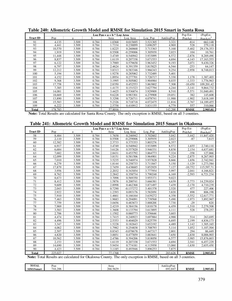
379
Table 240: Allometric Growth Model and RMSE for Simulation 2015 Smart in Santa Rosa
Tract ID Log Pop = a + b * Log Area Pop Est-
PopAct
(PopEst-
PopAct)2 Pop a b Area Log Area Log_Pop AntilogPop
91 4,135 3.509 0.784 1.0368 0.015695 3.521305 3,321 -814 662,148 92 4,441 3.509 0.784 1.7334 0.238899 3.696297 4,969 528 279,118
93 10,570 3.509 0.784 1.8225 0.260668 3.713363 5,168 -5,402 29,176,353
94 1,919 3.509 0.784 0.5508 -0.259006 3.305939 2,023 104 10,761
95 11,448 3.509 0.784 3.4749 0.540942 3.933099 8,572 -2,876 8,269,490
96 8,837 3.509 0.784 1.6119 0.207338 3.671553 4,694 -4,143 17,163,555
97 6,122 3.509 0.784 3.7989 0.579658 3.963452 9,193 3,071 9,430,326
98 6,797 3.509 0.784 2.4624 0.391359 3.815825 6,544 -253 64,147
99 12,212 3.509 0.784 3.8313 0.583346 3.966343 9,254 -2,958 8,748,013
100 5,194 3.509 0.784 1.9278 0.285062 3.732489 5,401
101 4,152 3.509 0.784 1.8954 0.277701 3.726717 5,330 1,178 1,387,403
102 9,368 3.509 0.784 3.1995 0.505082 3.904984 8,035 -1,333 1,776,963
103 17,758 3.509 0.784 2.8350 0.452553 3.863802 7,308 -10,450 109,201,42
104 7,385 3.509 0.784 1.4175 0.151523 3.627794 4,244 -3,141 9,864,732
105 14,081 3.509 0.784 3.4425 0.536874 3.929909 8,510 -5,571 31,040,491
106 18,669 3.509 0.784 9.6228 0.983301 4.279908 19,051 382 145,608
107 13,890 3.509 0.784 5.3298 0.726711 4.078741 11,988 -1,902 3,618,169
108 15,583 3.509 0.784 5.2326 0.718718 4.072475 11,816 -3,767 14,189,455
109 6,222 3.509 0.784 2.5758 0.410912 3.831155 6,779 557 310,066
Total 178,783 57.8016 142,200 RMSE 2,905.01
Note: Total Results are calculated for Santa Rosa County. The only exception is RMSE, based on all 3 counties.
Table 241: Allometric Growth Model and RMSE for Simulation 2015 Smart in Okaloosa
Tract ID Log Pop = a + b * Log Area Pop Est-
PopAct
(PopEst-
PopAct)2 Pop a b Area Log Area Log_Pop AntilogPop
58 8,484 3.509 0.784 1.7658 0.246942 3.702602 5,042 -3,442 11,847,420 59 2,110 3.509 0.784 0.5508 -0.259006 3.305939 2,023 -87 7,615
60 12,582 3.509 0.784 2.3733 0.375353 3.803276 6,357
61 6,917 3.509 0.784 3.4749 0.540942 3.933099 8,572 1,655 2,740,110
62 6,684 3.509 0.784 3.6126 0.557820 3.946331 8,838 2,154 4,637,681
63 7,682 3.509 0.784 2.8431 0.453792 3.864773 7,324 -358 127,866
64 12,099 3.509 0.784 3.8151 0.581506 3.964901 9,224 -2,875 8,267,903
65 7,010 3.509 0.784 3.5235 0.546974 3.937828 8,666 1,656 2,742,941
66 6,279 3.509 0.784 1.8144 0.258733 3.711847 5,150 -1,129 1,273,584
67 17,879 3.509 0.784 2.7459 0.438685 3.852929 7,127 -10,752 115,597,71
68 3,956 3.509 0.784 2.2032 0.343054 3.777954 5,997 2,041 4,166,821
69 8,762 3.509 0.784 2.2842 0.358734 3.790248 6,169 -2,593 6,721,234
70 8,673 3.509 0.784 3.7098 0.569350 3.955371 9,023
71 8,412 3.509 0.784 1.5876 0.200741 3.666381 4,639 -3,773 14,239,024
72 9,609 3.509 0.784 2.8998 0.462368 3.871497 7,439 -2,170 4,710,239
73 2,043 3.509 0.784 0.7290 -0.137272 3.401378 2,520 477 227,406
74 2,922 3.509 0.784 1.2393 0.093176 3.582050 3,820 898 806,198
75 7,910 3.509 0.784 1.4661 0.166164 3.639272 4,358 -3,552 12,617,771
76 7,463 3.509 0.784 1.9683 0.294091 3.739568 5,490 -1,973 3,892,967
77 7,759 3.509 0.784 3.0456 0.483673 3.888200 7,730 -29 820
78 7,969 3.509 0.784 2.4219 0.384156 3.810178 6,459 -1,510 2,279,508
79 3,583 3.509 0.784 1.3608 0.133794 3.613895 4,111 528 278,257
80 2,706 3.509 0.784 1.1502 0.060773 3.556646 3,603
81 4,474 3.509 0.784 1.7415 0.240923 3.697884 4,988 514 263,695
82 4,496 3.509 0.784 2.5353 0.404029 3.825759 6,695 2,199 4,836,173
83 3,347 3.509 0.784 1.5228 0.182643 3.652192 4,489 1,142 1,305,165
84 4,062 3.509 0.784 1.7982 0.254838 3.708793 5,114 1,052 1,107,504
85 2,507 3.509 0.784 0.8343 -0.078678 3.447317 2,801 294 86,449
86 4,820 3.509 0.784 3.0051 0.477859 3.883641 7,650 2,830 8,006,903
87 10,562 3.509 0.784 2.4786 0.394206 3.818058 6,577 -3,985 15,876,603
88 2,153 3.509 0.784 1.6119 0.207338 3.671553 4,694 2,541 6,457,229
89 14,690 3.509 0.784 5.9454 0.774181 4.115958 13,060 -1,630 2,655,450
90 4,423 3.509 0.784 3.1185 0.493946 3.896253 7,875
Total 225,027 77.1768 203,626 RMSE 2,905.01
Note: Total Results are calculated for Okaloosa County. The only exception is RMSE, based on all 3 counties.
TOTAL Pop
Area
AntilogPop SIM15smart 744,206 266.5629 692,847 RMSE 2,905.01
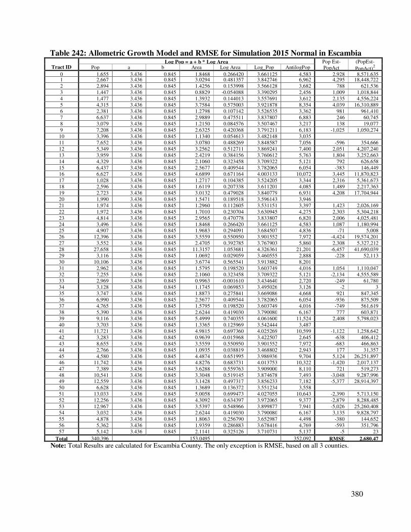
380
Table 242: Allometric Growth Model and RMSE for Simulation 2015 Normal in Escambia
Tract ID Log Pop = a + b * Log Area Pop Est-
PopAct
(PopEst-
PopAct)2 Pop a b Area Log Area Log_Pop AntilogPop
0 1,655 3.436 0.845 1.8468 0.266420 3.661125 4,583 2,928 8,571,635 1 2,667 3.436 0.845 3.0294 0.481357 3.842746 6,962 4,295 18,448,722
2 2,894 3.436 0.845 1.4256 0.153998 3.566128 3,682 788 621,536
3 1,447 3.436 0.845 0.8829 -0.054088 3.390295 2,456 1,009 1,018,844
4 1,477 3.436 0.845 1.3932 0.144013 3.557691 3,612 2,135 4,556,224
5 4,315 3.436 0.845 3.7584 0.575003 3.921878 8,354 4,039 16,310,889
6 2,381 3.436 0.845 1.2798 0.107142 3.526535 3,362 981 961,410
7 6,637 3.436 0.845 2.9889 0.475511 3.837807 6,883 246 60,745
8 3,079 3.436 0.845 1.2150 0.084576 3.507467 3,217 138 19,077
9 7,208 3.436 0.845 2.6325 0.420368 3.791211 6,183 -1,025 1,050,274
10 3,396 3.436 0.845 1.1340 0.054613 3.482148 3,035
11 7,652 3.436 0.845 3.0780 0.488269 3.848587 7,056 -596 354,666
12 5,349 3.436 0.845 3.2562 0.512711 3.869241 7,400 2,051 4,207,240
13 3,959 3.436 0.845 2.4219 0.384156 3.760612 5,763 1,804 3,252,663
14 4,329 3.436 0.845 2.1060 0.323458 3.709322 5,121 792 626,658
15 6,437 3.436 0.845 2.5677 0.409544 3.782065 6,054 -383 146,449
16 6,627 3.436 0.845 4.6899 0.671164 4.003133 10,072 3,445 11,870,823
17 1,028 3.436 0.845 1.2717 0.104385 3.524205 3,344 2,316 5,361,673
18 2,596 3.436 0.845 1.6119 0.207338 3.611201 4,085 1,489 2,217,363
19 2,723 3.436 0.845 3.0132 0.479028 3.840779 6,931 4,208 17,704,944
20 1,990 3.436 0.845 1.5471 0.189518 3.596143 3,946
21 1,974 3.436 0.845 1.2960 0.112605 3.531151 3,397 1,423 2,026,169
22 1,972 3.436 0.845 1.7010 0.230704 3.630945 4,275 2,303 5,304,218
23 4,814 3.436 0.845 2.9565 0.470778 3.833807 6,820 2,006 4,025,481
24 3,496 3.436 0.845 1.8468 0.266420 3.661125 4,583 1,087 1,180,994
25 4,907 3.436 0.845 1.9683 0.294091 3.684507 4,836 -71 5,008
26 12,396 3.436 0.845 3.5559 0.550950 3.901552 7,972 -4,424 19,574,201
27 3,552 3.436 0.845 2.4705 0.392785 3.767903 5,860 2,308 5,327,212
28 27,658 3.436 0.845 11.3157 1.053681 4.326361 21,201 -6,457 41,690,039
29 3,116 3.436 0.845 1.0692 0.029059 3.460555 2,888 -228 52,113
30 10,106 3.436 0.845 3.6774 0.565541 3.913882 8,201
31 2,962 3.436 0.845 1.5795 0.198520 3.603749 4,016 1,054 1,110,047
32 7,255 3.436 0.845 2.1060 0.323458 3.709322 5,121 -2,134 4,555,589
33 2,969 3.436 0.845 0.9963 -0.001610 3.434640 2,720 -249 61,780
34 3,128 3.436 0.845 1.1745 0.069853 3.495026 3,126 -2 3
35 3,747 3.436 0.845 1.8873 0.275841 3.669086 4,668 921 847,345
36 6,990 3.436 0.845 2.5677 0.409544 3.782065 6,054 -936 875,509
37 4,765 3.436 0.845 1.5795 0.198520 3.603749 4,016 -749 561,619
38 5,390 3.436 0.845 2.6244 0.419030 3.790080 6,167 777 603,871
39 9,116 3.436 0.845 5.4999 0.740355 4.061600 11,524 2,408 5,798,023
40 3,703 3.436 0.845 1.3365 0.125969 3.542444 3,487
41 11,721 3.436 0.845 4.9815 0.697360 4.025269 10,599 -1,122 1,258,642
42 3,283 3.436 0.845 0.9639 -0.015968 3.422507 2,645 -638 406,412
43 8,655 3.436 0.845 3.5559 0.550950 3.901552 7,972 -683 466,863
44 2,766 3.436 0.845 1.0935 0.038819 3.468802 2,943 177 31,357
45 4,580 3.436 0.845 4.4874 0.651995 3.986936 9,704 5,124 26,251,897
46 11,742 3.436 0.845 4.8276 0.683731 4.013753 10,322 -1,420 2,017,137
47 7,389 3.436 0.845 3.6288 0.559763 3.909000 8,110 721 519,273
48 10,541 3.436 0.845 3.3048 0.519145 3.874678 7,493 -3,048 9,287,996
49 12,559 3.436 0.845 3.1428 0.497317 3.856233 7,182 -5,377 28,914,397
50 6,628 3.436 0.845 1.3689 0.136372 3.551234 3,558
51 13,033 3.436 0.845 5.0058 0.699473 4.027055 10,643 -2,390 5,713,150
52 12,256 3.436 0.845 4.3092 0.634397 3.972065 9,377 -2,879 8,288,485
53 12,967 3.436 0.845 3.5397 0.548966 3.899877 7,941 -5,026 25,260,408
54 3,032 3.436 0.845 2.6244 0.419030 3.790080 6,167 3,135 9,828,797
55 4,878 3.436 0.845 1.8063 0.256790 3.652987 4,498 -380 144,652
56 5,362 3.436 0.845 1.9359 0.286883 3.678416 4,769 -593 351,796
57 5,142 3.436 0.845 2.1141 0.325126 3.710731 5,137 -5 23
Total 340,396 153.0495 352,092 RMSE 2,680.47
Note: Total Results are calculated for Escambia County. The only exception is RMSE, based on all 3 counties.

381
Table 243: Allometric Growth Model and RMSE for Simulation 2015 Normal in Sta. Rosa
Tract ID Log Pop = a + b * Log Area Pop Est-
PopAct
(PopEst-
PopAct)2 Pop a b Area Log Area Log_Pop AntilogPop
91 4,135 3.436 0.845 1.6605 0.220239 3.622102 4,189 54 2,907 92 4,441 3.436 0.845 2.2761 0.357191 3.737827 5,468 1,027 1,054,682
93 10,570 3.436 0.845 2.3166 0.364851 3.744299 5,550 -5,020 25,199,610
94 1,919 3.436 0.845 0.7695 -0.113791 3.339846 2,187 268 71,817
95 11,448 3.436 0.845 4.2768 0.631119 3.969296 9,317 -2,131 4,539,386
96 8,837 3.436 0.845 2.0007 0.301182 3.690499 4,903 -3,934 15,473,081
97 6,122 3.436 0.845 4.3416 0.637650 3.974814 9,437 3,315 10,986,363
98 6,797 3.436 0.845 3.2400 0.510545 3.867411 7,369 572 327,222
99 12,212 3.436 0.845 4.5927 0.662068 3.995448 9,896 -2,316 5,365,140
100 5,194 3.436 0.845 2.3976 0.379777 3.756911 5,714
101 4,152 3.436 0.845 2.1222 0.326786 3.712134 5,154 1,002 1,003,767
102 9,368 3.436 0.845 4.0500 0.607455 3.949299 8,898 -470 220,763
103 17,758 3.436 0.845 4.0338 0.605714 3.947829 8,868 -8,890 79,031,029
104 7,385 3.436 0.845 1.7577 0.244945 3.642978 4,395 -2,990 8,938,924
105 14,081 3.436 0.845 4.3011 0.633580 3.971375 9,362 -4,719 22,267,725
106 18,669 3.436 0.845 11.6316 1.065639 4.336465 21,700 3,031 9,188,660
107 13,890 3.436 0.845 6.3909 0.805562 4.116700 13,083 -807 651,610
108 15,583 3.436 0.845 6.3342 0.801692 4.113430 12,985 -2,598 6,751,532
109 6,222 3.436 0.845 3.0861 0.489410 3.849551 7,072 850 722,755
Total 178,783 71.5797 155,547 RMSE 2,680.47
Note: Total Results are calculated for Santa Rosa County. The only exception is RMSE, based on all 3 counties.
Table 244: Allometric Growth Model and RMSE for Simulation 2015 Normal in Okaloosa
Tract ID Log Pop = a + b * Log Area Pop Est-
PopAct
(PopEst-
PopAct)2 Pop a b Area Log Area Log_Pop AntilogPop
58 8,484 3.436 0.845 2.2680 0.355643 3.736518 5,452 -3,032 9,195,877 59 2,110 3.436 0.845 0.7290 -0.137272 3.320005 2,089 -21 428
60 12,582 3.436 0.845 3.0861 0.489410 3.849551 7,072
61 6,917 3.436 0.845 4.0905 0.611776 3.952951 8,973 2,056 4,228,273
62 6,684 3.436 0.845 4.3902 0.642484 3.978899 9,526 2,842 8,075,550
63 7,682 3.436 0.845 3.4425 0.536874 3.889658 7,756 74 5,531
64 12,099 3.436 0.845 4.6980 0.671913 4.003766 10,087 -2,012 4,047,726
65 7,010 3.436 0.845 3.6207 0.558793 3.908180 8,094 1,084 1,175,723
66 6,279 3.436 0.845 2.0979 0.321785 3.707908 5,104 -1,175 1,380,695
67 17,879 3.436 0.845 3.4587 0.538913 3.891381 7,787 -10,092 101,844,40
68 3,956 3.436 0.845 2.4381 0.387052 3.763059 5,795 1,839 3,382,171
69 8,762 3.436 0.845 2.6487 0.423033 3.793463 6,215 -2,547 6,485,637
70 8,673 3.436 0.845 4.0419 0.606586 3.948565 8,883
71 8,412 3.436 0.845 1.7820 0.250908 3.648017 4,446 -3,966 15,725,295
72 9,609 3.436 0.845 3.3048 0.519145 3.874678 7,493 -2,116 4,475,854
73 2,043 3.436 0.845 0.9477 -0.023329 3.416287 2,608 565 319,085
74 2,922 3.436 0.845 1.4337 0.156458 3.568207 3,700 778 605,357
75 7,910 3.436 0.845 1.5795 0.198520 3.603749 4,016 -3,894 15,166,449
76 7,463 3.436 0.845 2.2599 0.354089 3.735205 5,435 -2,028 4,112,487
77 7,759 3.436 0.845 3.5073 0.544973 3.896502 7,880 121 14,535
78 7,969 3.436 0.845 2.7135 0.433530 3.802333 6,344 -1,625 2,642,072
79 3,583 3.436 0.845 1.4499 0.161338 3.572331 3,735 152 23,209
80 2,706 3.436 0.845 1.2960 0.112605 3.531151 3,397
81 4,474 3.436 0.845 1.9602 0.292300 3.682994 4,819 345 119,308
82 4,496 3.436 0.845 2.7297 0.436115 3.804517 6,376 1,880 3,532,678
83 3,347 3.436 0.845 1.6686 0.222352 3.623888 4,206 859 738,187
84 4,062 3.436 0.845 2.0331 0.308159 3.696394 4,970 908 825,249
85 2,507 3.436 0.845 0.8748 -0.058091 3.386913 2,437 -70 4,855
86 4,820 3.436 0.845 3.3696 0.527578 3.881804 7,617 2,797 7,825,147
87 10,562 3.436 0.845 2.9565 0.470778 3.833807 6,820 -3,742 13,999,868
88 2,153 3.436 0.845 1.9521 0.290502 3.681474 4,803 2,650 7,020,253
89 14,690 3.436 0.845 7.2414 0.859823 4.162550 14,540 -150 22,644
90 4,423 3.436 0.845 3.4020 0.531734 3.885315 7,679
Total 225,027 89.4726 206,157 RMSE 2,680.47
Note: Total Results are calculated for Okaloosa County. The only exception is RMSE, based on all 3 counties.
TOTAL Pop
Area
AntilogPop SIM15norm 744,206 314.1018 713,796 RMSE 2,680.47
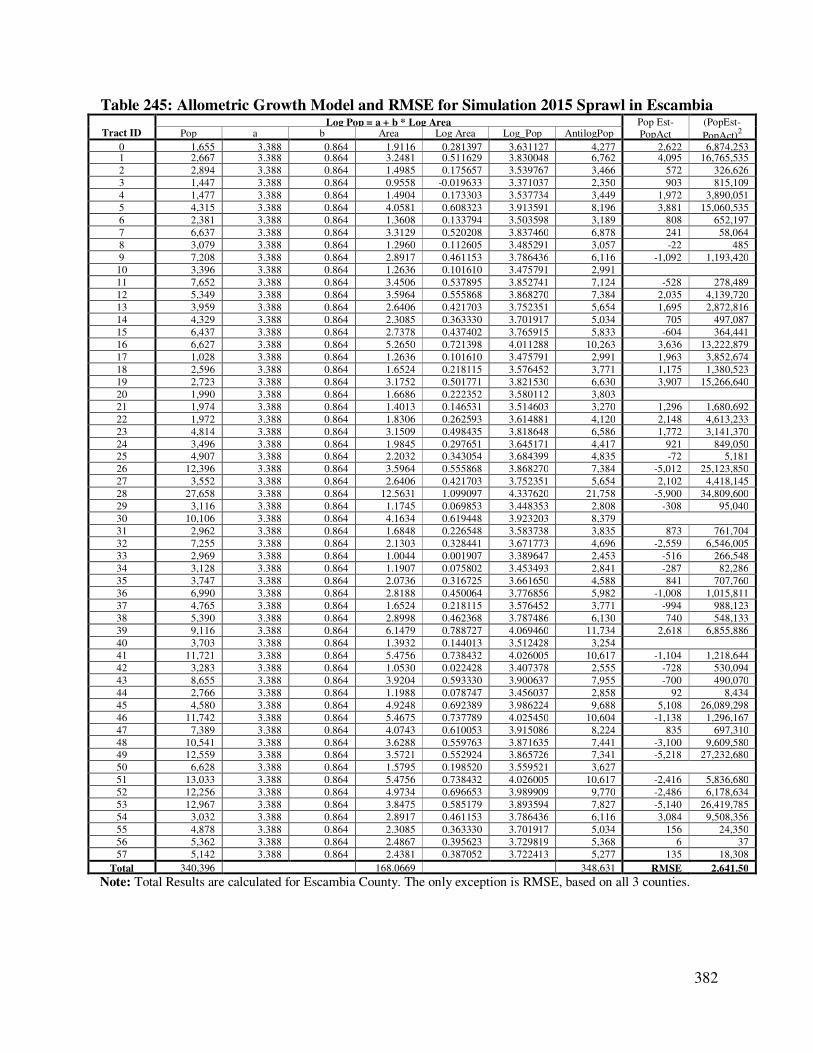
382
Table 245: Allometric Growth Model and RMSE for Simulation 2015 Sprawl in Escambia
Tract ID Log Pop = a + b * Log Area Pop Est-
PopAct
(PopEst-
PopAct)2 Pop a b Area Log Area Log_Pop AntilogPop
0 1,655 3.388 0.864 1.9116 0.281397 3.631127 4,277 2,622 6,874,253 1 2,667 3.388 0.864 3.2481 0.511629 3.830048 6,762 4,095 16,765,535
2 2,894 3.388 0.864 1.4985 0.175657 3.539767 3,466 572 326,626
3 1,447 3.388 0.864 0.9558 -0.019633 3.371037 2,350 903 815,109
4 1,477 3.388 0.864 1.4904 0.173303 3.537734 3,449 1,972 3,890,051
5 4,315 3.388 0.864 4.0581 0.608323 3.913591 8,196 3,881 15,060,535
6 2,381 3.388 0.864 1.3608 0.133794 3.503598 3,189 808 652,197
7 6,637 3.388 0.864 3.3129 0.520208 3.837460 6,878 241 58,064
8 3,079 3.388 0.864 1.2960 0.112605 3.485291 3,057 -22 485
9 7,208 3.388 0.864 2.8917 0.461153 3.786436 6,116 -1,092 1,193,420
10 3,396 3.388 0.864 1.2636 0.101610 3.475791 2,991
11 7,652 3.388 0.864 3.4506 0.537895 3.852741 7,124 -528 278,489
12 5,349 3.388 0.864 3.5964 0.555868 3.868270 7,384 2,035 4,139,720
13 3,959 3.388 0.864 2.6406 0.421703 3.752351 5,654 1,695 2,872,816
14 4,329 3.388 0.864 2.3085 0.363330 3.701917 5,034 705 497,087
15 6,437 3.388 0.864 2.7378 0.437402 3.765915 5,833 -604 364,441
16 6,627 3.388 0.864 5.2650 0.721398 4.011288 10,263 3,636 13,222,879
17 1,028 3.388 0.864 1.2636 0.101610 3.475791 2,991 1,963 3,852,674
18 2,596 3.388 0.864 1.6524 0.218115 3.576452 3,771 1,175 1,380,523
19 2,723 3.388 0.864 3.1752 0.501771 3.821530 6,630 3,907 15,266,640
20 1,990 3.388 0.864 1.6686 0.222352 3.580112 3,803
21 1,974 3.388 0.864 1.4013 0.146531 3.514603 3,270 1,296 1,680,692
22 1,972 3.388 0.864 1.8306 0.262593 3.614881 4,120 2,148 4,613,233
23 4,814 3.388 0.864 3.1509 0.498435 3.818648 6,586 1,772 3,141,370
24 3,496 3.388 0.864 1.9845 0.297651 3.645171 4,417 921 849,050
25 4,907 3.388 0.864 2.2032 0.343054 3.684399 4,835 -72 5,181
26 12,396 3.388 0.864 3.5964 0.555868 3.868270 7,384 -5,012 25,123,850
27 3,552 3.388 0.864 2.6406 0.421703 3.752351 5,654 2,102 4,418,145
28 27,658 3.388 0.864 12.5631 1.099097 4.337620 21,758 -5,900 34,809,600
29 3,116 3.388 0.864 1.1745 0.069853 3.448353 2,808 -308 95,040
30 10,106 3.388 0.864 4.1634 0.619448 3.923203 8,379
31 2,962 3.388 0.864 1.6848 0.226548 3.583738 3,835 873 761,704
32 7,255 3.388 0.864 2.1303 0.328441 3.671773 4,696 -2,559 6,546,005
33 2,969 3.388 0.864 1.0044 0.001907 3.389647 2,453 -516 266,548
34 3,128 3.388 0.864 1.1907 0.075802 3.453493 2,841 -287 82,286
35 3,747 3.388 0.864 2.0736 0.316725 3.661650 4,588 841 707,760
36 6,990 3.388 0.864 2.8188 0.450064 3.776856 5,982 -1,008 1,015,811
37 4,765 3.388 0.864 1.6524 0.218115 3.576452 3,771 -994 988,123
38 5,390 3.388 0.864 2.8998 0.462368 3.787486 6,130 740 548,133
39 9,116 3.388 0.864 6.1479 0.788727 4.069460 11,734 2,618 6,855,886
40 3,703 3.388 0.864 1.3932 0.144013 3.512428 3,254
41 11,721 3.388 0.864 5.4756 0.738432 4.026005 10,617 -1,104 1,218,644
42 3,283 3.388 0.864 1.0530 0.022428 3.407378 2,555 -728 530,094
43 8,655 3.388 0.864 3.9204 0.593330 3.900637 7,955 -700 490,070
44 2,766 3.388 0.864 1.1988 0.078747 3.456037 2,858 92 8,434
45 4,580 3.388 0.864 4.9248 0.692389 3.986224 9,688 5,108 26,089,298
46 11,742 3.388 0.864 5.4675 0.737789 4.025450 10,604 -1,138 1,296,167
47 7,389 3.388 0.864 4.0743 0.610053 3.915086 8,224 835 697,310
48 10,541 3.388 0.864 3.6288 0.559763 3.871635 7,441 -3,100 9,609,580
49 12,559 3.388 0.864 3.5721 0.552924 3.865726 7,341 -5,218 27,232,680
50 6,628 3.388 0.864 1.5795 0.198520 3.559521 3,627
51 13,033 3.388 0.864 5.4756 0.738432 4.026005 10,617 -2,416 5,836,680
52 12,256 3.388 0.864 4.9734 0.696653 3.989909 9,770 -2,486 6,178,634
53 12,967 3.388 0.864 3.8475 0.585179 3.893594 7,827 -5,140 26,419,785
54 3,032 3.388 0.864 2.8917 0.461153 3.786436 6,116 3,084 9,508,356
55 4,878 3.388 0.864 2.3085 0.363330 3.701917 5,034 156 24,350
56 5,362 3.388 0.864 2.4867 0.395623 3.729819 5,368 6 37
57 5,142 3.388 0.864 2.4381 0.387052 3.722413 5,277 135 18,308
Total 340,396 168.0669 348,631 RMSE 2,641.50
Note: Total Results are calculated for Escambia County. The only exception is RMSE, based on all 3 counties.
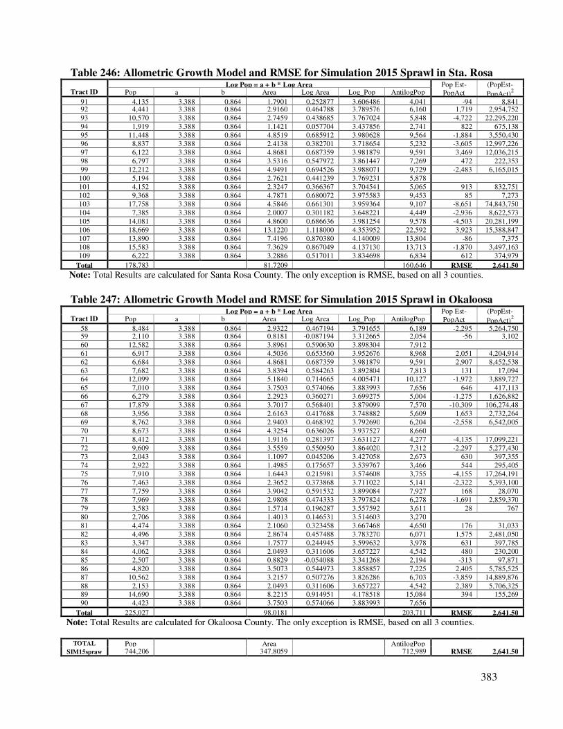
383
Table 246: Allometric Growth Model and RMSE for Simulation 2015 Sprawl in Sta. Rosa
Tract ID Log Pop = a + b * Log Area Pop Est-
PopAct
(PopEst-
PopAct)2 Pop a b Area Log Area Log_Pop AntilogPop
91 4,135 3.388 0.864 1.7901 0.252877 3.606486 4,041 -94 8,841 92 4,441 3.388 0.864 2.9160 0.464788 3.789576 6,160 1,719 2,954,752
93 10,570 3.388 0.864 2.7459 0.438685 3.767024 5,848 -4,722 22,295,220
94 1,919 3.388 0.864 1.1421 0.057704 3.437856 2,741 822 675,138
95 11,448 3.388 0.864 4.8519 0.685912 3.980628 9,564 -1,884 3,550,430
96 8,837 3.388 0.864 2.4138 0.382701 3.718654 5,232 -3,605 12,997,226
97 6,122 3.388 0.864 4.8681 0.687359 3.981879 9,591 3,469 12,036,215
98 6,797 3.388 0.864 3.5316 0.547972 3.861447 7,269 472 222,353
99 12,212 3.388 0.864 4.9491 0.694526 3.988071 9,729 -2,483 6,165,015
100 5,194 3.388 0.864 2.7621 0.441239 3.769231 5,878
101 4,152 3.388 0.864 2.3247 0.366367 3.704541 5,065 913 832,751
102 9,368 3.388 0.864 4.7871 0.680072 3.975583 9,453 85 7,273
103 17,758 3.388 0.864 4.5846 0.661301 3.959364 9,107 -8,651 74,843,750
104 7,385 3.388 0.864 2.0007 0.301182 3.648221 4,449 -2,936 8,622,573
105 14,081 3.388 0.864 4.8600 0.686636 3.981254 9,578 -4,503 20,281,199
106 18,669 3.388 0.864 13.1220 1.118000 4.353952 22,592 3,923 15,388,847
107 13,890 3.388 0.864 7.4196 0.870380 4.140009 13,804 -86 7,375
108 15,583 3.388 0.864 7.3629 0.867049 4.137130 13,713 -1,870 3,497,163
109 6,222 3.388 0.864 3.2886 0.517011 3.834698 6,834 612 374,979
Total 178,783 81.7209 160,646 RMSE 2,641.50
Note: Total Results are calculated for Santa Rosa County. The only exception is RMSE, based on all 3 counties.
Table 247: Allometric Growth Model and RMSE for Simulation 2015 Sprawl in Okaloosa
Tract ID Log Pop = a + b * Log Area Pop Est-
PopAct
(PopEst-
PopAct)2 Pop a b Area Log Area Log_Pop AntilogPop
58 8,484 3.388 0.864 2.9322 0.467194 3.791655 6,189 -2,295 5,264,750 59 2,110 3.388 0.864 0.8181 -0.087194 3.312665 2,054 -56 3,102
60 12,582 3.388 0.864 3.8961 0.590630 3.898304 7,912
61 6,917 3.388 0.864 4.5036 0.653560 3.952676 8,968 2,051 4,204,914
62 6,684 3.388 0.864 4.8681 0.687359 3.981879 9,591 2,907 8,452,538
63 7,682 3.388 0.864 3.8394 0.584263 3.892804 7,813 131 17,094
64 12,099 3.388 0.864 5.1840 0.714665 4.005471 10,127 -1,972 3,889,727
65 7,010 3.388 0.864 3.7503 0.574066 3.883993 7,656 646 417,113
66 6,279 3.388 0.864 2.2923 0.360271 3.699275 5,004 -1,275 1,626,882
67 17,879 3.388 0.864 3.7017 0.568401 3.879099 7,570 -10,309 106,274,48
68 3,956 3.388 0.864 2.6163 0.417688 3.748882 5,609 1,653 2,732,264
69 8,762 3.388 0.864 2.9403 0.468392 3.792690 6,204 -2,558 6,542,005
70 8,673 3.388 0.864 4.3254 0.636026 3.937527 8,660
71 8,412 3.388 0.864 1.9116 0.281397 3.631127 4,277 -4,135 17,099,221
72 9,609 3.388 0.864 3.5559 0.550950 3.864020 7,312 -2,297 5,277,430
73 2,043 3.388 0.864 1.1097 0.045206 3.427058 2,673 630 397,355
74 2,922 3.388 0.864 1.4985 0.175657 3.539767 3,466 544 295,405
75 7,910 3.388 0.864 1.6443 0.215981 3.574608 3,755 -4,155 17,264,191
76 7,463 3.388 0.864 2.3652 0.373868 3.711022 5,141 -2,322 5,393,100
77 7,759 3.388 0.864 3.9042 0.591532 3.899084 7,927 168 28,070
78 7,969 3.388 0.864 2.9808 0.474333 3.797824 6,278 -1,691 2,859,370
79 3,583 3.388 0.864 1.5714 0.196287 3.557592 3,611 28 767
80 2,706 3.388 0.864 1.4013 0.146531 3.514603 3,270
81 4,474 3.388 0.864 2.1060 0.323458 3.667468 4,650 176 31,033
82 4,496 3.388 0.864 2.8674 0.457488 3.783270 6,071 1,575 2,481,050
83 3,347 3.388 0.864 1.7577 0.244945 3.599632 3,978 631 397,785
84 4,062 3.388 0.864 2.0493 0.311606 3.657227 4,542 480 230,200
85 2,507 3.388 0.864 0.8829 -0.054088 3.341268 2,194 -313 97,871
86 4,820 3.388 0.864 3.5073 0.544973 3.858857 7,225 2,405 5,785,525
87 10,562 3.388 0.864 3.2157 0.507276 3.826286 6,703 -3,859 14,889,876
88 2,153 3.388 0.864 2.0493 0.311606 3.657227 4,542 2,389 5,706,325
89 14,690 3.388 0.864 8.2215 0.914951 4.178518 15,084 394 155,269
90 4,423 3.388 0.864 3.7503 0.574066 3.883993 7,656
Total 225,027 98.0181 203,711 RMSE 2,641.50
Note: Total Results are calculated for Okaloosa County. The only exception is RMSE, based on all 3 counties.
TOTAL Pop
Area
AntilogPop SIM15spraw 744,206 347.8059 712,989 RMSE 2,641.50

384
Table 248: Allometric Growth Model and RMSE for Simulation 2020 Smart in Escambia
Tract ID Log Pop = a + b * Log Area Pop Est-
PopAct
(PopEst-
PopAct)2 Pop a b Area Log Area Log_Pop AntilogPop
0 1,531 3.522 0.807 1.7010 0.230704 3.708178 5,107 3,576 12,788,829 1 2,523 3.522 0.807 2.7540 0.439964 3.877051 7,534 5,011 25,114,517
2 2,710 3.522 0.807 1.3284 0.123329 3.621526 4,183 1,473 2,170,823
3 1,379 3.522 0.807 0.8181 -0.087194 3.451635 2,829 1,450 2,102,534
4 1,338 3.522 0.807 1.3284 0.123329 3.621526 4,183 2,845 8,096,137
5 4,040 3.522 0.807 3.3777 0.528621 3.948597 8,884 4,844 23,462,088
6 2,284 3.522 0.807 1.1016 0.042024 3.555913 3,597 1,313 1,723,379
7 6,673 3.522 0.807 2.5515 0.406796 3.850284 7,084 411 168,994
8 3,074 3.522 0.807 1.1259 0.051500 3.563560 3,661 587 344,179
9 7,522 3.522 0.807 2.3328 0.367878 3.818877 6,590 -932 868,858
10 3,514 3.522 0.807 0.9639 -0.015968 3.509114 3,229
11 7,938 3.522 0.807 2.7621 0.441239 3.878080 7,552 -386 148,752
12 5,346 3.522 0.807 2.9322 0.467194 3.899025 7,925 2,579 6,653,684
13 3,948 3.522 0.807 2.1708 0.336620 3.793652 6,218 2,270 5,152,996
14 4,189 3.522 0.807 1.8225 0.260668 3.732359 5,400 1,211 1,465,465
15 6,682 3.522 0.807 2.3409 0.369383 3.820092 6,608 -74 5,427
16 6,742 3.522 0.807 4.0014 0.602212 4.007985 10,186 3,444 11,858,129
17 930 3.522 0.807 1.1340 0.054613 3.566073 3,682 2,752 7,572,988
18 2,501 3.522 0.807 1.4661 0.166164 3.656094 4,530 2,029 4,116,664
19 2,575 3.522 0.807 2.6163 0.417688 3.859074 7,229 4,654 21,659,038
20 1,846 3.522 0.807 1.3608 0.133794 3.629972 4,266
21 1,882 3.522 0.807 1.1664 0.066848 3.575946 3,767 1,885 3,551,601
22 1,860 3.522 0.807 1.5471 0.189518 3.674941 4,731 2,871 8,241,915
23 4,637 3.522 0.807 2.6406 0.421703 3.862314 7,283 2,646 7,001,645
24 3,288 3.522 0.807 1.6362 0.213836 3.694566 4,950 1,662 2,760,758
25 4,707 3.522 0.807 1.7982 0.254838 3.727654 5,341 634 402,450
26 12,998 3.522 0.807 3.4263 0.534825 3.953604 8,987 -4,011 16,089,890
27 3,830 3.522 0.807 2.1951 0.341454 3.797554 6,274 2,444 5,973,780
28 31,877 3.522 0.807 9.5904 0.981837 4.314342 20,623 -11,254 126,662,78
29 3,315 3.522 0.807 0.8667 -0.062131 3.471860 2,964 -351 123,288
30 10,795 3.522 0.807 3.1023 0.491684 3.918789 8,294
31 3,002 3.522 0.807 1.2960 0.112605 3.612872 4,101 1,099 1,207,437
32 7,601 3.522 0.807 1.7739 0.248929 3.722886 5,283 -2,318 5,372,831
33 3,003 3.522 0.807 0.8424 -0.074482 3.461893 2,897 -106 11,314
34 3,133 3.522 0.807 1.1259 0.051500 3.563560 3,661 528 278,434
35 3,578 3.522 0.807 1.7253 0.236865 3.713150 5,166 1,588 2,521,568
36 6,887 3.522 0.807 2.1789 0.338237 3.794958 6,237 -650 422,841
37 4,671 3.522 0.807 1.4175 0.151523 3.644279 4,408 -263 68,969
38 5,521 3.522 0.807 2.2680 0.355643 3.809004 6,442 921 847,783
39 9,382 3.522 0.807 4.8681 0.687359 4.076699 11,932 2,550 6,500,520
40 4,022 3.522 0.807 1.0854 0.035590 3.550721 3,554
41 12,636 3.522 0.807 4.2525 0.628644 4.029316 10,698 -1,938 3,754,567
42 3,573 3.522 0.807 0.8343 -0.078678 3.458507 2,874 -699 488,413
43 9,262 3.522 0.807 3.0861 0.489410 3.916954 8,260 -1,002 1,005,002
44 2,925 3.522 0.807 0.9477 -0.023329 3.503173 3,185 260 67,844
45 4,507 3.522 0.807 3.7260 0.571243 3.982993 9,616 5,109 26,101,547
46 12,423 3.522 0.807 4.0095 0.603090 4.008694 10,202 -2,221 4,931,955
47 7,772 3.522 0.807 3.1347 0.496196 3.922430 8,364 592 350,832
48 11,075 3.522 0.807 2.9079 0.463579 3.896109 7,872 -3,203 10,256,475
49 13,865 3.522 0.807 2.6730 0.426999 3.866588 7,355 -6,510 42,378,891
50 7,276 3.522 0.807 1.2393 0.093176 3.597193 3,955
51 14,633 3.522 0.807 4.2363 0.626987 4.027978 10,665 -3,968 15,741,631
52 13,734 3.522 0.807 3.6531 0.562662 3.976068 9,464 -4,270 18,234,175
53 14,347 3.522 0.807 2.9727 0.473151 3.903833 8,014 -6,333 40,110,725
54 2,909 3.522 0.807 2.2113 0.344648 3.800131 6,311 3,402 11,576,816
55 4,960 3.522 0.807 1.2798 0.107142 3.608464 4,059 -901 811,050
56 5,391 3.522 0.807 1.4742 0.168556 3.658025 4,550 -841 707,041
57 5,111 3.522 0.807 1.8063 0.256790 3.729229 5,361 250 62,399
Total 355,673 132.9858 368,178 RMSE 3,460.02
Note: Total Results are calculated for Escambia County. The only exception is RMSE, based on all 3 counties.

385
Table 249: Allometric Growth Model and RMSE for Simulation 2020 Smart in Santa Rosa
Tract ID Log Pop = a + b * Log Area Pop Est-
PopAct
(PopEst-
PopAct)2 Pop a b Area Log Area Log_Pop AntilogPop
91 4,113 3.522 0.807 1.0530 0.022428 3.540100 3,468 -645 415,813 92 4,325 3.522 0.807 1.7820 0.250908 3.724483 5,303 978 955,550
93 11,750 3.522 0.807 1.8792 0.273973 3.743096 5,535 -6,215 38,629,617
94 1,737 3.522 0.807 0.5508 -0.259006 3.312982 2,056 319 101,637
95 12,226 3.522 0.807 3.5235 0.546974 3.963408 9,192 -3,034 9,205,384
96 9,529 3.522 0.807 1.6443 0.215981 3.696297 4,969 -4,560 20,790,708
97 5,830 3.522 0.807 3.8394 0.584263 3.993501 9,851 4,021 16,172,128
98 7,206 3.522 0.807 2.4948 0.397036 3.842408 6,957 -249 62,114
99 13,293 3.522 0.807 3.8637 0.587003 3.995712 9,902 -3,391 11,500,610
100 5,582 3.522 0.807 1.9521 0.290502 3.756435 5,707
101 4,332 3.522 0.807 1.8954 0.277701 3.746105 5,573 1,241 1,540,577
102 9,933 3.522 0.807 3.2967 0.518079 3.940090 8,711 -1,222 1,492,202
103 20,362 3.522 0.807 2.8917 0.461153 3.894151 7,837 -12,525 156,875,25
104 8,827 3.522 0.807 1.4256 0.153998 3.646276 4,429 -4,398 19,345,054
105 15,693 3.522 0.807 3.5478 0.549959 3.965817 9,243 -6,450 41,601,384
106 22,046 3.522 0.807 9.7119 0.987304 4.318754 20,833 -1,213 1,471,057
107 16,193 3.522 0.807 5.4027 0.732611 4.113217 12,978 -3,215 10,334,460
108 17,853 3.522 0.807 5.3460 0.728029 4.109519 12,868 -4,985 24,847,769
109 6,103 3.522 0.807 2.5920 0.413635 3.855803 7,175 1,072 1,148,530
Total 196,933 58.6926 152,588 RMSE 3,460.02
Note: Total Results are calculated for Santa Rosa County. The only exception is RMSE, based on all 3 counties.
Table 250: Allometric Growth Model and RMSE for Simulation 2020 Smart in Okaloosa
Tract ID Log Pop = a + b * Log Area Pop Est-
PopAct
(PopEst-
PopAct)2 Pop a b Area Log Area Log_Pop AntilogPop
58 8,888 3.522 0.807 1.7820 0.250908 3.724483 5,303 -3,585 12,855,649 59 2,159 3.522 0.807 0.5508 -0.259006 3.312982 2,056 -103 10,649
60 13,918 3.522 0.807 2.3976 0.379777 3.828480 6,737
61 7,232 3.522 0.807 3.5397 0.548966 3.965016 9,226 1,994 3,976,246
62 6,933 3.522 0.807 3.6369 0.560731 3.974510 9,430 2,497 6,234,848
63 8,402 3.522 0.807 2.8917 0.461153 3.894151 7,837 -565 319,208
64 13,614 3.522 0.807 3.8637 0.587003 3.995712 9,902 -3,712 13,780,836
65 7,432 3.522 0.807 3.5235 0.546974 3.963408 9,192 1,760 3,097,468
66 6,771 3.522 0.807 1.8306 0.262593 3.733913 5,419 -1,352 1,828,114
67 21,299 3.522 0.807 2.7945 0.446304 3.882167 7,624 -13,675 187,013,05
68 4,074 3.522 0.807 2.2194 0.346236 3.801412 6,330 2,256 5,090,089
69 9,052 3.522 0.807 2.2842 0.358734 3.811498 6,479 -2,573 6,621,061
70 8,836 3.522 0.807 3.7503 0.574066 3.985271 9,667
71 8,548 3.522 0.807 1.5876 0.200741 3.683998 4,831 -3,717 13,819,312
72 9,946 3.522 0.807 2.9322 0.467194 3.899025 7,925 -2,021 4,082,527
73 2,052 3.522 0.807 0.7290 -0.137272 3.411221 2,578 526 276,290
74 2,929 3.522 0.807 1.2393 0.093176 3.597193 3,955 1,026 1,053,553
75 8,772 3.522 0.807 1.4661 0.166164 3.656094 4,530 -4,242 17,994,934
76 8,214 3.522 0.807 1.9764 0.295875 3.760771 5,765 -2,449 5,999,442
77 8,069 3.522 0.807 3.0699 0.487124 3.915109 8,224 155 24,179
78 8,071 3.522 0.807 2.4543 0.389928 3.836672 6,865 -1,206 1,453,252
79 3,606 3.522 0.807 1.3770 0.138934 3.634120 4,306 700 490,634
80 2,757 3.522 0.807 1.1502 0.060773 3.571044 3,724
81 4,490 3.522 0.807 1.7658 0.246942 3.721282 5,264 774 598,437
82 4,503 3.522 0.807 2.5596 0.408172 3.851395 7,102 2,599 6,756,010
83 3,417 3.522 0.807 1.5390 0.187239 3.673102 4,711 1,294 1,674,112
84 4,068 3.522 0.807 1.8144 0.258733 3.730798 5,380 1,312 1,721,841
85 2,606 3.522 0.807 0.8343 -0.078678 3.458507 2,874 268 71,896
86 4,911 3.522 0.807 3.0375 0.482516 3.911391 8,154 3,243 10,519,477
87 11,521 3.522 0.807 2.5272 0.402640 3.846930 7,030 -4,491 20,172,739
88 2,208 3.522 0.807 1.6362 0.213836 3.694566 4,950 2,742 7,516,112
89 16,605 3.522 0.807 6.0669 0.782967 4.153854 14,251 -2,354 5,539,942
90 4,782 3.522 0.807 3.1347 0.496196 3.922430 8,364
Total 240,685 77.9625 215,985 RMSE 3,460.02
Note: Total Results are calculated for Okaloosa County. The only exception is RMSE, based on all 3 counties.
TOTAL Pop
Area
AntilogPop SIM20smart 793,291 269.6409 736,751 RMSE 3,460.02
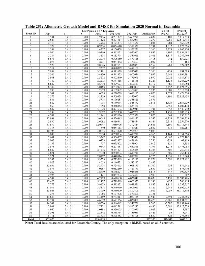
386
Table 251: Allometric Growth Model and RMSE for Simulation 2020 Normal in Escambia
Tract ID Log Pop = a + b * Log Area Pop Est-
PopAct
(PopEst-
PopAct)2 Pop a b Area Log Area Log_Pop AntilogPop
0 1,531 3.410 0.909 1.9116 0.281397 3.665790 4,632 3,101 9,617,613 1 2,523 3.410 0.909 3.1428 0.497317 3.862061 7,279 4,756 22,617,814
2 2,710 3.410 0.909 1.4904 0.173303 3.567532 3,694 984 968,849
3 1,379 3.410 0.909 0.9234 -0.034610 3.378539 2,391 1,012 1,023,696
4 1,338 3.410 0.909 1.4337 0.156458 3.552221 3,566 2,228 4,965,420
5 4,040 3.410 0.909 3.9366 0.595121 3.950965 8,932 4,892 23,934,992
6 2,284 3.410 0.909 1.3608 0.133794 3.531619 3,401 1,117 1,247,906
7 6,673 3.410 0.909 3.2076 0.506180 3.870118 7,415 742 550,733
8 3,074 3.410 0.909 1.2231 0.087462 3.489503 3,087 13 163
9 7,522 3.410 0.909 2.8026 0.447561 3.816833 6,559 -963 927,502
10 3,514 3.410 0.909 1.2312 0.090329 3.492109 3,105
11 7,938 3.410 0.909 3.2481 0.511629 3.875071 7,500 -438 191,695
12 5,346 3.410 0.909 3.4830 0.541953 3.902636 7,992 2,646 6,999,391
13 3,948 3.410 0.909 2.5272 0.402640 3.775999 5,970 2,022 4,089,878
14 4,189 3.410 0.909 2.2275 0.347818 3.726166 5,323 1,134 1,286,229
15 6,682 3.410 0.909 2.6892 0.429623 3.800527 6,317 -365 133,050
16 6,742 3.410 0.909 5.0463 0.702973 4.049003 11,194 4,452 19,824,255
17 930 3.410 0.909 1.2879 0.109882 3.509883 3,235 2,305 5,313,320
18 2,501 3.410 0.909 1.6605 0.220239 3.610197 4,076 1,575 2,479,530
19 2,575 3.410 0.909 3.2319 0.509458 3.873097 7,466 4,891 23,923,438
20 1,846 3.410 0.909 1.5714 0.196287 3.588425 3,876
21 1,882 3.410 0.909 1.4094 0.149034 3.545472 3,511 1,629 2,654,729
22 1,860 3.410 0.909 1.7658 0.246942 3.634470 4,310 2,450 6,002,138
23 4,637 3.410 0.909 3.1023 0.491684 3.856941 7,194 2,557 6,535,719
24 3,288 3.410 0.909 1.9602 0.292300 3.675701 4,739 1,451 2,105,855
25 4,707 3.410 0.909 2.1141 0.325126 3.705539 5,076 369 136,312
26 12,998 3.410 0.909 3.6045 0.556845 3.916172 8,245 -4,753 22,594,353
27 3,830 3.410 0.909 2.6082 0.416341 3.788454 6,144 2,314 5,354,770
28 31,877 3.410 0.909 12.0447 1.080796 4.392444 24,686 -7,191 51,716,344
29 3,315 3.410 0.909 1.1340 0.054613 3.459643 2,882 -433 187,781
30 10,795 3.410 0.909 4.0095 0.603090 3.958209 9,083
31 3,002 3.410 0.909 1.7010 0.230704 3.619710 4,166 1,164 1,354,694
32 7,601 3.410 0.909 2.3247 0.366367 3.743028 5,534 -2,067 4,273,102
33 3,003 3.410 0.909 1.0773 0.032337 3.439394 2,750 -253 63,813
34 3,133 3.410 0.909 1.1907 0.075802 3.478904 3,012 -121 14,558
35 3,578 3.410 0.909 1.9845 0.297651 3.680565 4,793 1,215 1,475,083
36 6,887 3.410 0.909 2.7216 0.434824 3.805255 6,386 -501 250,613
37 4,671 3.410 0.909 1.7010 0.230704 3.619710 4,166 -505 255,113
38 5,521 3.410 0.909 2.8107 0.448814 3.817972 6,576 1,055 1,113,363
39 9,382 3.410 0.909 5.9373 0.773589 4.113192 12,978 3,596 12,927,912
40 4,022 3.410 0.909 1.4013 0.146531 3.543197 3,493
41 12,636 3.410 0.909 5.2974 0.724063 4.068173 11,700 -936 876,742
42 3,573 3.410 0.909 1.0287 0.012289 3.421170 2,637 -936 875,410
43 9,262 3.410 0.909 3.8799 0.588821 3.945238 8,815 -447 199,527
44 2,925 3.410 0.909 1.1421 0.057704 3.462453 2,900 -25 607
45 4,507 3.410 0.909 4.7709 0.678600 4.026848 10,638 6,131 37,585,466
46 12,423 3.410 0.909 5.2407 0.719389 4.063925 11,586 -837 700,955
47 7,772 3.410 0.909 3.9123 0.592432 3.948521 8,882 1,110 1,232,557
48 11,075 3.410 0.909 3.5478 0.549959 3.909913 8,127 -2,948 8,692,625
49 13,865 3.410 0.909 3.3939 0.530699 3.892405 7,806 -6,059 36,716,516
50 7,276 3.410 0.909 1.5066 0.177998 3.571800 3,731
51 14,633 3.410 0.909 5.4189 0.733911 4.077125 11,943 -2,690 7,234,356
52 13,734 3.410 0.909 4.6899 0.671164 4.020088 10,473 -3,261 10,631,511
53 14,347 3.410 0.909 3.8556 0.586092 3.942758 8,765 -5,582 31,157,444
54 2,909 3.410 0.909 2.7702 0.442511 3.812243 6,490 3,581 12,823,338
55 4,960 3.410 0.909 2.0898 0.320105 3.700975 5,023 63 3,987
56 5,391 3.410 0.909 2.2842 0.358734 3.736089 5,446 55 3,041
57 5,111 3.410 0.909 2.3733 0.375353 3.751196 5,639 528 278,694
Total 355,673 163.4418 377,336 RMSE 3,095.31
Note: Total Results are calculated for Escambia County. The only exception is RMSE, based on all 3 counties.

387
Table 252: Allometric Growth Model and RMSE for Simulation 2020 Normal in Sta. Rosa
Tract ID Log Pop = a + b * Log Area Pop Est-
PopAct
(PopEst-
PopAct)2 Pop a b Area Log Area Log_Pop AntilogPop
91 4,113 3.410 0.909 1.9278 0.285062 3.669121 4,668 555 307,912 92 4,325 3.410 0.909 2.5920 0.413635 3.785994 6,109 1,784 3,183,865
93 11,750 3.410 0.909 2.5839 0.412276 3.784759 6,092 -5,658 32,013,167
94 1,737 3.410 0.909 0.8991 -0.046192 3.368011 2,334 597 355,836
95 12,226 3.410 0.909 4.6575 0.668153 4.017351 10,408 -1,818 3,306,547
96 9,529 3.410 0.909 2.2275 0.347818 3.726166 5,323 -4,206 17,689,422
97 5,830 3.410 0.909 4.5198 0.655119 4.005503 10,128 4,298 18,468,730
98 7,206 3.410 0.909 3.6693 0.564583 3.923206 8,379 1,173 1,376,561
99 13,293 3.410 0.909 4.9815 0.697360 4.043900 11,064 -2,229 4,969,782
100 5,582 3.410 0.909 2.5758 0.410912 3.783519 6,075
101 4,332 3.410 0.909 2.3004 0.361803 3.738879 5,481 1,149 1,320,765
102 9,933 3.410 0.909 4.4469 0.648057 3.999084 9,979 46 2,110
103 20,362 3.410 0.909 4.6008 0.662833 4.012516 10,292 -10,070 101,397,38
104 8,827 3.410 0.909 1.9359 0.286883 3.670777 4,686 -4,141 17,150,179
105 15,693 3.410 0.909 4.6413 0.666640 4.015975 10,375 -5,318 28,284,344
106 22,046 3.410 0.909 12.6360 1.101610 4.411363 25,785 3,739 13,978,348
107 16,193 3.410 0.909 7.0713 0.849499 4.182195 15,212 -981 961,776
108 17,853 3.410 0.909 6.9174 0.839943 4.173508 14,911 -2,942 8,655,098
109 6,103 3.410 0.909 3.3129 0.520208 3.882869 7,636 1,533 2,350,275
Total 196,933 78.4971 174,936 RMSE 3,095.31
Note: Total Results are calculated for Santa Rosa County. The only exception is RMSE, based on all 3 counties.
Table 253: Allometric Growth Model and RMSE for Simulation 2020 Normal in Okaloosa
Tract ID Log Pop = a + b * Log Area Pop Est-
PopAct
(PopEst-
PopAct)2 Pop a b Area Log Area Log_Pop AntilogPop
58 8,888 3.410 0.909 2.5758 0.410912 3.783519 6,075 -2,813 7,915,106 59 2,159 3.410 0.909 0.7938 -0.100289 3.318837 2,084 -75 5,669
60 13,918 3.410 0.909 3.5964 0.555868 3.915284 8,228
61 7,232 3.410 0.909 4.4550 0.648848 3.999803 9,995 2,763 7,636,683
62 6,933 3.410 0.909 4.7061 0.672661 4.021449 10,506 3,573 12,768,333
63 8,402 3.410 0.909 3.7989 0.579658 3.936909 8,648 246 60,451
64 13,614 3.410 0.909 5.1030 0.707826 4.053413 11,309 -2,305 5,314,317
65 7,432 3.410 0.909 3.6531 0.562662 3.921459 8,346 914 834,728
66 6,771 3.410 0.909 2.2437 0.350965 3.729027 5,358 -1,413 1,995,722
67 21,299 3.410 0.909 3.6855 0.566496 3.924945 8,413 -12,886 166,051,81
68 4,074 3.410 0.909 2.5353 0.404029 3.777263 5,988 1,914 3,662,388
69 9,052 3.410 0.909 2.8917 0.461153 3.829188 6,748 -2,304 5,307,470
70 8,836 3.410 0.909 4.1634 0.619448 3.973078 9,399
71 8,548 3.410 0.909 1.8630 0.270213 3.655623 4,525 -4,023 16,184,118
72 9,946 3.410 0.909 3.4506 0.537895 3.898946 7,924 -2,022 4,088,356
73 2,052 3.410 0.909 1.0206 0.008856 3.418050 2,618 566 320,903
74 2,929 3.410 0.909 1.4904 0.173303 3.567532 3,694 765 585,686
75 8,772 3.410 0.909 1.6605 0.220239 3.610197 4,076 -4,696 22,055,680
76 8,214 3.410 0.909 2.4057 0.381241 3.756548 5,709 -2,505 6,275,786
77 8,069 3.410 0.909 3.6774 0.565541 3.924077 8,396 327 106,982
78 8,071 3.410 0.909 2.8269 0.451310 3.820241 6,611 -1,460 2,132,754
79 3,606 3.410 0.909 1.5309 0.184947 3.578117 3,785 179 32,200
80 2,757 3.410 0.909 1.3446 0.128593 3.526891 3,364
81 4,490 3.410 0.909 2.0331 0.308159 3.690116 4,899 409 167,363
82 4,503 3.410 0.909 2.8026 0.447561 3.816833 6,559 2,056 4,226,852
83 3,417 3.410 0.909 1.7253 0.236865 3.625310 4,220 803 644,770
84 4,068 3.410 0.909 2.1384 0.330089 3.710051 5,129 1,061 1,126,176
85 2,606 3.410 0.909 0.9153 -0.038437 3.375061 2,372 -234 54,893
86 4,911 3.410 0.909 3.4992 0.543969 3.904468 8,025 3,114 9,699,593
87 11,521 3.410 0.909 3.1671 0.500662 3.865102 7,330 -4,191 17,564,823
88 2,208 3.410 0.909 2.0412 0.309886 3.691686 4,917 2,709 7,337,808
89 16,605 3.410 0.909 7.8894 0.897044 4.225413 16,804 199 39,606
90 4,782 3.410 0.909 3.6045 0.556845 3.916172 8,245
Total 240,685 95.2884 220,299 RMSE 3,095.31
Note: Total Results are calculated for Okaloosa County. The only exception is RMSE, based on all 3 counties.
TOTAL Pop
Area
AntilogPop SIM20norm 793,291 337.2273 772,571 RMSE 3,095.31

388
Table 254: Allometric Growth Model and RMSE for Simulation 2020 Sprawl in Escambia
Tract ID Log Pop = a + b * Log Area Pop Est-
PopAct
(PopEst-
PopAct)2 Pop a b Area Log Area Log_Pop AntilogPop
0 1,531 3.340 0.944 1.9764 0.295875 3.619306 4,162 2,631 6,922,352 1 2,523 3.340 0.944 3.3453 0.524435 3.835067 6,840 4,317 18,637,931
2 2,710 3.340 0.944 1.5471 0.189518 3.518905 3,303 593 351,620
3 1,379 3.340 0.944 1.0044 0.001907 3.341800 2,197 818 668,875
4 1,338 3.340 0.944 1.5309 0.184947 3.514590 3,270 1,932 3,733,848
5 4,040 3.340 0.944 4.2120 0.624488 3.929517 8,502 4,462 19,908,730
6 2,284 3.340 0.944 1.4661 0.166164 3.496858 3,139 855 731,855
7 6,673 3.340 0.944 3.5721 0.552924 3.861960 7,277 604 364,968
8 3,074 3.340 0.944 1.4013 0.146531 3.478325 3,008 -66 4,313
9 7,522 3.340 0.944 3.1185 0.493946 3.806285 6,402 -1,120 1,255,420
10 3,514 3.340 0.944 1.4256 0.153998 3.485374 3,058
11 7,938 3.340 0.944 3.6855 0.566496 3.874773 7,495 -443 196,234
12 5,346 3.340 0.944 3.9609 0.597794 3.904317 8,023 2,677 7,164,413
13 3,948 3.340 0.944 2.9160 0.464788 3.778759 6,008 2,060 4,245,281
14 4,189 3.340 0.944 2.5110 0.399847 3.717455 5,217 1,028 1,057,635
15 6,682 3.340 0.944 2.9484 0.469586 3.783290 6,071 -611 372,820
16 6,742 3.340 0.944 5.6781 0.754203 4.051968 11,271 4,529 20,513,067
17 930 3.340 0.944 1.2879 0.109882 3.443729 2,778 1,848 3,415,021
18 2,501 3.340 0.944 1.7010 0.230704 3.557785 3,612 1,111 1,235,007
19 2,575 3.340 0.944 3.3372 0.523382 3.834073 6,825 4,250 18,058,516
20 1,846 3.340 0.944 1.7334 0.238899 3.565520 3,677
21 1,882 3.340 0.944 1.4904 0.173303 3.503598 3,189 1,307 1,707,162
22 1,860 3.340 0.944 1.9359 0.286883 3.610817 4,081 2,221 4,934,965
23 4,637 3.340 0.944 3.3129 0.520208 3.831077 6,778 2,141 4,582,217
24 3,288 3.340 0.944 2.0574 0.313319 3.635773 4,323 1,035 1,070,971
25 4,707 3.340 0.944 2.3571 0.372378 3.691525 4,915 208 43,270
26 12,998 3.340 0.944 3.6612 0.563623 3.872061 7,448 -5,550 30,798,527
27 3,830 3.340 0.944 2.8188 0.450064 3.764861 5,819 1,989 3,956,777
28 31,877 3.340 0.944 13.7700 1.138934 4.415154 26,011 -5,866 34,412,352
29 3,315 3.340 0.944 1.3770 0.138934 3.471154 2,959 -356 126,694
30 10,795 3.340 0.944 4.6332 0.665881 3.968592 9,302
31 3,002 3.340 0.944 1.8468 0.266420 3.591500 3,904 902 813,451
32 7,601 3.340 0.944 2.3490 0.370883 3.690114 4,899 -2,702 7,300,430
33 3,003 3.340 0.944 1.0773 0.032337 3.370526 2,347 -656 430,246
34 3,133 3.340 0.944 1.2150 0.084576 3.419840 2,629 -504 253,715
35 3,578 3.340 0.944 2.2113 0.344648 3.665347 4,628 1,050 1,101,472
36 6,887 3.340 0.944 3.0294 0.481357 3.794401 6,229 -658 433,298
37 4,671 3.340 0.944 1.7577 0.244945 3.571228 3,726 -945 893,268
38 5,521 3.340 0.944 3.2076 0.506180 3.817834 6,574 1,053 1,108,950
39 9,382 3.340 0.944 6.7635 0.830171 4.123682 13,295 3,913 15,310,024
40 4,022 3.340 0.944 1.5309 0.184947 3.514590 3,270
41 12,636 3.340 0.944 5.9859 0.777129 4.073610 11,847 -789 622,443
42 3,573 3.340 0.944 1.1583 0.063821 3.400247 2,513 -1,060 1,122,930
43 9,262 3.340 0.944 4.2606 0.629471 3.934220 8,594 -668 445,562
44 2,925 3.340 0.944 1.2474 0.096006 3.430629 2,695 -230 52,699
45 4,507 3.340 0.944 5.3379 0.727370 4.026638 10,633 6,126 37,522,439
46 12,423 3.340 0.944 5.9940 0.777717 4.074165 11,862 -561 314,516
47 7,772 3.340 0.944 4.3254 0.636026 3.940409 8,718 946 894,610
48 11,075 3.340 0.944 3.8880 0.589726 3.896702 7,883 -3,192 10,187,698
49 13,865 3.340 0.944 4.0338 0.605714 3.911794 8,162 -5,703 32,524,688
50 7,276 3.340 0.944 1.8387 0.264511 3.589698 3,888
51 14,633 3.340 0.944 6.1560 0.789299 4.085098 12,165 -2,468 6,092,991
52 13,734 3.340 0.944 5.3946 0.731959 4.030970 10,739 -2,995 8,969,183
53 14,347 3.340 0.944 4.3416 0.637650 3.941941 8,749 -5,598 31,341,438
54 2,909 3.340 0.944 3.1509 0.498435 3.810522 6,464 3,555 12,640,240
55 4,960 3.340 0.944 2.9484 0.469586 3.783290 6,071 1,111 1,235,232
56 5,391 3.340 0.944 3.0942 0.490548 3.803078 6,354 963 928,228
57 5,111 3.340 0.944 2.8755 0.458713 3.773025 5,930 819 670,107
Total 355,673 182.7927 371,730 RMSE 3,027.78
Note: Total Results are calculated for Escambia County. The only exception is RMSE, based on all 3 counties.
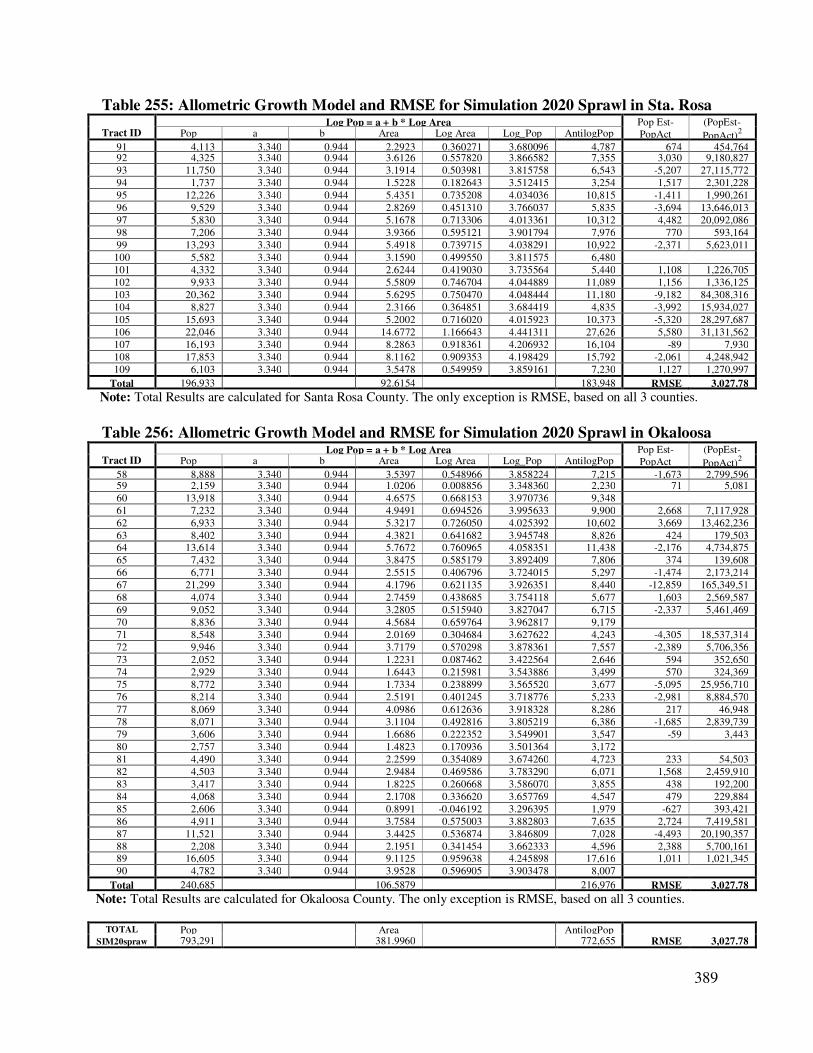
389
Table 255: Allometric Growth Model and RMSE for Simulation 2020 Sprawl in Sta. Rosa
Tract ID Log Pop = a + b * Log Area Pop Est-
PopAct
(PopEst-
PopAct)2 Pop a b Area Log Area Log_Pop AntilogPop
91 4,113 3.340 0.944 2.2923 0.360271 3.680096 4,787 674 454,764 92 4,325 3.340 0.944 3.6126 0.557820 3.866582 7,355 3,030 9,180,827
93 11,750 3.340 0.944 3.1914 0.503981 3.815758 6,543 -5,207 27,115,772
94 1,737 3.340 0.944 1.5228 0.182643 3.512415 3,254 1,517 2,301,228
95 12,226 3.340 0.944 5.4351 0.735208 4.034036 10,815 -1,411 1,990,261
96 9,529 3.340 0.944 2.8269 0.451310 3.766037 5,835 -3,694 13,646,013
97 5,830 3.340 0.944 5.1678 0.713306 4.013361 10,312 4,482 20,092,086
98 7,206 3.340 0.944 3.9366 0.595121 3.901794 7,976 770 593,164
99 13,293 3.340 0.944 5.4918 0.739715 4.038291 10,922 -2,371 5,623,011
100 5,582 3.340 0.944 3.1590 0.499550 3.811575 6,480
101 4,332 3.340 0.944 2.6244 0.419030 3.735564 5,440 1,108 1,226,705
102 9,933 3.340 0.944 5.5809 0.746704 4.044889 11,089 1,156 1,336,125
103 20,362 3.340 0.944 5.6295 0.750470 4.048444 11,180 -9,182 84,308,316
104 8,827 3.340 0.944 2.3166 0.364851 3.684419 4,835 -3,992 15,934,027
105 15,693 3.340 0.944 5.2002 0.716020 4.015923 10,373 -5,320 28,297,687
106 22,046 3.340 0.944 14.6772 1.166643 4.441311 27,626 5,580 31,131,562
107 16,193 3.340 0.944 8.2863 0.918361 4.206932 16,104 -89 7,930
108 17,853 3.340 0.944 8.1162 0.909353 4.198429 15,792 -2,061 4,248,942
109 6,103 3.340 0.944 3.5478 0.549959 3.859161 7,230 1,127 1,270,997
Total 196,933 92.6154 183,948 RMSE 3,027.78
Note: Total Results are calculated for Santa Rosa County. The only exception is RMSE, based on all 3 counties.
Table 256: Allometric Growth Model and RMSE for Simulation 2020 Sprawl in Okaloosa
Tract ID Log Pop = a + b * Log Area Pop Est-
PopAct
(PopEst-
PopAct)2 Pop a b Area Log Area Log_Pop AntilogPop
58 8,888 3.340 0.944 3.5397 0.548966 3.858224 7,215 -1,673 2,799,596 59 2,159 3.340 0.944 1.0206 0.008856 3.348360 2,230 71 5,081
60 13,918 3.340 0.944 4.6575 0.668153 3.970736 9,348
61 7,232 3.340 0.944 4.9491 0.694526 3.995633 9,900 2,668 7,117,928
62 6,933 3.340 0.944 5.3217 0.726050 4.025392 10,602 3,669 13,462,236
63 8,402 3.340 0.944 4.3821 0.641682 3.945748 8,826 424 179,503
64 13,614 3.340 0.944 5.7672 0.760965 4.058351 11,438 -2,176 4,734,875
65 7,432 3.340 0.944 3.8475 0.585179 3.892409 7,806 374 139,608
66 6,771 3.340 0.944 2.5515 0.406796 3.724015 5,297 -1,474 2,173,214
67 21,299 3.340 0.944 4.1796 0.621135 3.926351 8,440 -12,859 165,349,51
68 4,074 3.340 0.944 2.7459 0.438685 3.754118 5,677 1,603 2,569,587
69 9,052 3.340 0.944 3.2805 0.515940 3.827047 6,715 -2,337 5,461,469
70 8,836 3.340 0.944 4.5684 0.659764 3.962817 9,179
71 8,548 3.340 0.944 2.0169 0.304684 3.627622 4,243 -4,305 18,537,314
72 9,946 3.340 0.944 3.7179 0.570298 3.878361 7,557 -2,389 5,706,356
73 2,052 3.340 0.944 1.2231 0.087462 3.422564 2,646 594 352,650
74 2,929 3.340 0.944 1.6443 0.215981 3.543886 3,499 570 324,369
75 8,772 3.340 0.944 1.7334 0.238899 3.565520 3,677 -5,095 25,956,710
76 8,214 3.340 0.944 2.5191 0.401245 3.718776 5,233 -2,981 8,884,570
77 8,069 3.340 0.944 4.0986 0.612636 3.918328 8,286 217 46,948
78 8,071 3.340 0.944 3.1104 0.492816 3.805219 6,386 -1,685 2,839,739
79 3,606 3.340 0.944 1.6686 0.222352 3.549901 3,547 -59 3,443
80 2,757 3.340 0.944 1.4823 0.170936 3.501364 3,172
81 4,490 3.340 0.944 2.2599 0.354089 3.674260 4,723 233 54,503
82 4,503 3.340 0.944 2.9484 0.469586 3.783290 6,071 1,568 2,459,910
83 3,417 3.340 0.944 1.8225 0.260668 3.586070 3,855 438 192,200
84 4,068 3.340 0.944 2.1708 0.336620 3.657769 4,547 479 229,884
85 2,606 3.340 0.944 0.8991 -0.046192 3.296395 1,979 -627 393,421
86 4,911 3.340 0.944 3.7584 0.575003 3.882803 7,635 2,724 7,419,581
87 11,521 3.340 0.944 3.4425 0.536874 3.846809 7,028 -4,493 20,190,357
88 2,208 3.340 0.944 2.1951 0.341454 3.662333 4,596 2,388 5,700,161
89 16,605 3.340 0.944 9.1125 0.959638 4.245898 17,616 1,011 1,021,345
90 4,782 3.340 0.944 3.9528 0.596905 3.903478 8,007
Total 240,685 106.5879 216,976 RMSE 3,027.78
Note: Total Results are calculated for Okaloosa County. The only exception is RMSE, based on all 3 counties.
TOTAL Pop
Area
AntilogPop SIM20spraw 793,291 381.9960 772,655 RMSE 3,027.78
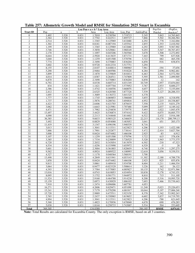
390
Table 257: Allometric Growth Model and RMSE for Simulation 2025 Smart in Escambia
Tract ID Log Pop = a + b * Log Area Pop Est-
PopAct
(PopEst-
PopAct)2 Pop a b Area Log Area Log_Pop AntilogPop
0 1,402 3.528 0.831 1.7010 0.230704 3.719715 5,245 3,843 14,765,845 1 2,364 3.528 0.831 2.7702 0.442511 3.895727 7,866 5,502 30,266,584
2 2,514 3.528 0.831 1.3365 0.125969 3.632680 4,292 1,778 3,162,004
3 1,302 3.528 0.831 0.8181 -0.087194 3.455542 2,855 1,553 2,410,502
4 1,199 3.528 0.831 1.3365 0.125969 3.632680 4,292 3,093 9,567,902
5 3,746 3.528 0.831 3.3858 0.529661 3.968149 9,293 5,547 30,767,453
6 2,170 3.528 0.831 1.1097 0.045206 3.565566 3,678 1,508 2,272,892
7 6,644 3.528 0.831 2.5920 0.413635 3.871731 7,443 799 637,926
8 3,040 3.528 0.831 1.1259 0.051500 3.570796 3,722 682 465,358
9 7,774 3.528 0.831 2.3490 0.370883 3.836204 6,858 -916 838,874
10 3,602 3.528 0.831 0.9720 -0.012334 3.517751 3,294
11 8,155 3.528 0.831 2.8107 0.448814 3.900965 7,961 -194 37,656
12 5,290 3.528 0.831 2.9484 0.469586 3.918226 8,284 2,994 8,962,461
13 3,899 3.528 0.831 2.1870 0.339849 3.810414 6,463 2,564 6,572,584
14 4,014 3.528 0.831 1.8387 0.264511 3.747809 5,595 1,581 2,499,905
15 6,870 3.528 0.831 2.3490 0.370883 3.836204 6,858 -12 142
16 6,792 3.528 0.831 4.0338 0.605714 4.031349 10,749 3,957 15,654,044
17 834 3.528 0.831 1.1421 0.057704 3.575952 3,767 2,933 8,600,277
18 2,386 3.528 0.831 1.4742 0.168556 3.668070 4,657 2,271 5,155,694
19 2,412 3.528 0.831 2.6325 0.420368 3.877326 7,539 5,127 26,288,333
20 1,695 3.528 0.831 1.3689 0.136372 3.641325 4,378
21 1,777 3.528 0.831 1.1745 0.069853 3.586048 3,855 2,078 4,318,950
22 1,737 3.528 0.831 1.5876 0.200741 3.694816 4,952 3,215 10,338,807
23 4,423 3.528 0.831 2.6406 0.421703 3.878435 7,558 3,135 9,831,279
24 3,062 3.528 0.831 1.6443 0.215981 3.707480 5,099 2,037 4,149,142
25 4,471 3.528 0.831 1.7982 0.254838 3.739770 5,493 1,022 1,043,470
26 13,497 3.528 0.831 3.4425 0.536874 3.974142 9,422 -4,075 16,605,775
27 4,090 3.528 0.831 2.2113 0.344648 3.814402 6,522 2,432 5,916,188
28 36,385 3.528 0.831 9.6633 0.985125 4.346639 22,215 -14,170 200,799,13
29 3,492 3.528 0.831 0.8829 -0.054088 3.483052 3,041 -451 203,173
30 11,419 3.528 0.831 3.1347 0.496196 3.940339 8,716
31 3,013 3.528 0.831 1.3041 0.115311 3.623823 4,206 1,193 1,422,188
32 7,886 3.528 0.831 1.7901 0.252877 3.738141 5,472 -2,414 5,827,704
33 3,008 3.528 0.831 0.8424 -0.074482 3.466106 2,925 -83 6,912
34 3,107 3.528 0.831 1.1259 0.051500 3.570796 3,722 615 378,436
35 3,385 3.528 0.831 1.7334 0.238899 3.726525 5,328 1,943 3,773,375
36 6,720 3.528 0.831 2.2032 0.343054 3.813078 6,502 -218 47,323
37 4,534 3.528 0.831 1.4256 0.153998 3.655972 4,529 -5 28
38 5,601 3.528 0.831 2.3004 0.361803 3.828659 6,740 1,139 1,297,275
39 9,562 3.528 0.831 4.8924 0.689522 4.100993 12,618 3,056 9,339,531
40 4,327 3.528 0.831 1.1178 0.048364 3.568191 3,700
41 13,490 3.528 0.831 4.2849 0.631941 4.053143 11,302 -2,188 4,788,778
42 3,850 3.528 0.831 0.8424 -0.074482 3.466106 2,925 -925 855,876
43 9,815 3.528 0.831 3.0861 0.489410 3.934700 8,604 -1,211 1,466,554
44 3,064 3.528 0.831 0.9477 -0.023329 3.508614 3,226 162 26,122
45 4,393 3.528 0.831 3.7584 0.575003 4.005827 10,135 5,742 32,971,566
46 13,016 3.528 0.831 4.0743 0.610053 4.034954 10,838 -2,178 4,743,151
47 8,095 3.528 0.831 3.1752 0.501771 3.944972 8,810 715 511,105
48 11,524 3.528 0.831 2.9160 0.464788 3.914238 8,208 -3,316 10,995,720
49 15,159 3.528 0.831 2.6973 0.430929 3.886102 7,693 -7,466 55,739,443
50 7,910 3.528 0.831 1.2474 0.096006 3.607781 4,053
51 16,271 3.528 0.831 4.2606 0.629471 4.051090 11,248 -5,023 25,226,653
52 15,241 3.528 0.831 3.7179 0.570298 4.001917 10,044 -5,197 27,006,240
53 15,720 3.528 0.831 2.9889 0.475511 3.923150 8,378 -7,342 53,902,243
54 2,765 3.528 0.831 2.2437 0.350965 3.819652 6,602 3,837 14,719,795
55 4,994 3.528 0.831 1.3041 0.115311 3.623823 4,206 -788 621,645
56 5,368 3.528 0.831 1.4823 0.170936 3.670048 4,678 -690 476,283
57 5,030 3.528 0.831 1.8144 0.258733 3.743007 5,534 504 253,605
Total 369,305 134.0388 384,185 RMSE 4,074.41
Note: Total Results are calculated for Escambia County. The only exception is RMSE, based on all 3 counties.
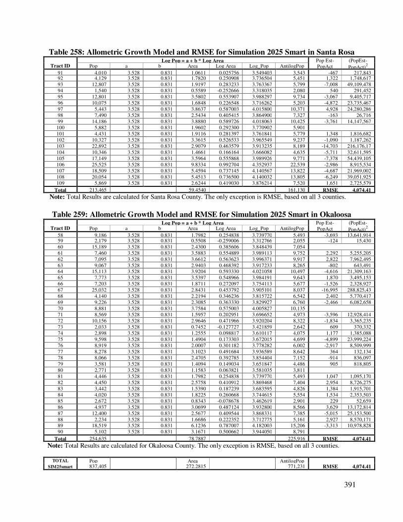
391
Table 258: Allometric Growth Model and RMSE for Simulation 2025 Smart in Santa Rosa
Tract ID Log Pop = a + b * Log Area Pop Est-
PopAct
(PopEst-
PopAct)2 Pop a b Area Log Area Log_Pop AntilogPop
91 4,010 3.528 0.831 1.0611 0.025756 3.549403 3,543 -467 217,843 92 4,129 3.528 0.831 1.7820 0.250908 3.736504 5,451 1,322 1,748,617
93 12,807 3.528 0.831 1.9197 0.283233 3.763367 5,799 -7,008 49,109,478
94 1,540 3.528 0.831 0.5589 -0.252666 3.318035 2,080 540 291,452
95 12,801 3.528 0.831 3.5802 0.553907 3.988297 9,734 -3,067 9,405,717
96 10,075 3.528 0.831 1.6848 0.226548 3.716262 5,203 -4,872 23,735,467
97 5,443 3.528 0.831 3.8637 0.587003 4.015800 10,371 4,928 24,280,286
98 7,490 3.528 0.831 2.5434 0.405415 3.864900 7,327 -163 26,716
99 14,186 3.528 0.831 3.8880 0.589726 4.018063 10,425 -3,761 14,147,567
100 5,882 3.528 0.831 1.9602 0.292300 3.770902 5,901
101 4,431 3.528 0.831 1.9116 0.281397 3.761841 5,779 1,348 1,816,682
102 10,327 3.528 0.831 3.3615 0.526533 3.965549 9,237 -1,090 1,187,262
103 22,892 3.528 0.831 2.9079 0.463579 3.913235 8,189 -14,703 216,176,17
104 10,346 3.528 0.831 1.4661 0.166164 3.666082 4,635 -5,711 32,611,595
105 17,149 3.528 0.831 3.5964 0.555868 3.989926 9,771 -7,378 54,439,105
106 25,525 3.528 0.831 9.8334 0.992704 4.352937 22,539 -2,986 8,915,534
107 18,509 3.528 0.831 5.4594 0.737145 4.140567 13,822 -4,687 21,969,002
108 20,054 3.528 0.831 5.4513 0.736500 4.140032 13,805 -6,249 39,051,925
109 5,869 3.528 0.831 2.6244 0.419030 3.876214 7,520 1,651 2,725,579
Total 213,465 59.4540 161,130 RMSE 4,074.41
Note: Total Results are calculated for Santa Rosa County. The only exception is RMSE, based on all 3 counties.
Table 259: Allometric Growth Model and RMSE for Simulation 2025 Smart in Okaloosa
Tract ID Log Pop = a + b * Log Area Pop Est-
PopAct
(PopEst-
PopAct)2 Pop a b Area Log Area Log_Pop AntilogPop
58 9,186 3.528 0.831 1.7982 0.254838 3.739770 5,493 -3,693 13,641,914 59 2,179 3.528 0.831 0.5508 -0.259006 3.312766 2,055 -124 15,430
60 15,189 3.528 0.831 2.4300 0.385606 3.848439 7,054
61 7,460 3.528 0.831 3.5883 0.554889 3.989113 9,752 2,292 5,255,205
62 7,095 3.528 0.831 3.6612 0.563623 3.996371 9,917 2,822 7,962,495
63 9,067 3.528 0.831 2.9403 0.468392 3.917233 8,265 -802 643,491
64 15,113 3.528 0.831 3.9204 0.593330 4.021058 10,497 -4,616 21,309,163
65 7,773 3.528 0.831 3.5397 0.548966 3.984191 9,643 1,870 3,495,153
66 7,203 3.528 0.831 1.8711 0.272097 3.754113 5,677 -1,526 2,328,927
67 25,032 3.528 0.831 2.8431 0.453792 3.905101 8,037 -16,995 288,825,43
68 4,140 3.528 0.831 2.2194 0.346236 3.815722 6,542 2,402 5,770,417
69 9,226 3.528 0.831 2.3085 0.363330 3.829927 6,760 -2,466 6,082,658
70 8,881 3.528 0.831 3.7584 0.575003 4.005827 10,135
71 8,569 3.528 0.831 1.5957 0.202951 3.696652 4,973 -3,596 12,928,414
72 10,156 3.528 0.831 2.9646 0.471966 3.920204 8,322 -1,834 3,365,235
73 2,033 3.528 0.831 0.7452 -0.127727 3.421859 2,642 609 370,332
74 2,898 3.528 0.831 1.2555 0.098817 3.610117 4,075 1,177 1,385,088
75 9,598 3.528 0.831 1.4904 0.173303 3.672015 4,699 -4,899 23,999,224
76 8,919 3.528 0.831 2.0007 0.301182 3.778282 6,002 -2,917 8,509,999
77 8,278 3.528 0.831 3.1023 0.491684 3.936589 8,642 364 132,134
78 8,066 3.528 0.831 2.4705 0.392785 3.854404 7,152 -914 836,097
79 3,581 3.528 0.831 1.4094 0.149034 3.651847 4,486 905 818,805
80 2,771 3.528 0.831 1.1583 0.063821 3.581035 3,811
81 4,446 3.528 0.831 1.7982 0.254838 3.739770 5,493 1,047 1,095,170
82 4,450 3.528 0.831 2.5758 0.410912 3.869468 7,404 2,954 8,726,275
83 3,442 3.528 0.831 1.5390 0.187239 3.683595 4,826 1,384 1,915,701
84 4,020 3.528 0.831 1.8225 0.260668 3.744615 5,554 1,534 2,353,503
85 2,672 3.528 0.831 0.8343 -0.078678 3.462619 2,901 229 52,659
86 4,937 3.528 0.831 3.0699 0.487124 3.932800 8,566 3,629 13,172,814
87 12,400 3.528 0.831 2.5677 0.409544 3.868331 7,385 -5,015 25,153,500
88 2,234 3.528 0.831 1.6686 0.222352 3.712775 5,161 2,927 8,570,171
89 18,519 3.528 0.831 6.1236 0.787007 4.182003 15,206 -3,313 10,978,828
90 5,102 3.528 0.831 3.1671 0.500662 3.944050 8,791
Total 254,635 78.7887 225,916 RMSE 4,074.41
Note: Total Results are calculated for Okaloosa County. The only exception is RMSE, based on all 3 counties.
TOTAL Pop
Area
AntilogPop SIM25smart 837,405 272.2815 771,231 RMSE 4,074.41
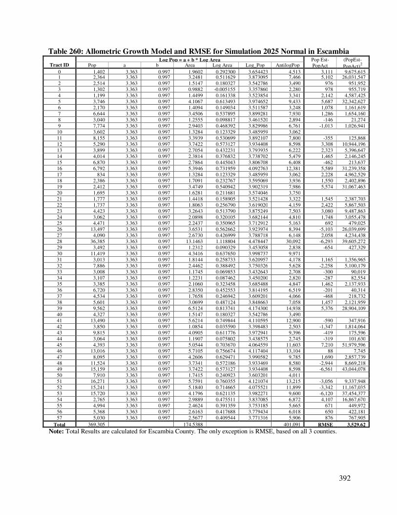
392
Table 260: Allometric Growth Model and RMSE for Simulation 2025 Normal in Escambia
Tract ID Log Pop = a + b * Log Area Pop Est-
PopAct
(PopEst-
PopAct)2 Pop a b Area Log Area Log_Pop AntilogPop
0 1,402 3.363 0.997 1.9602 0.292300 3.654423 4,513 3,111 9,675,615 1 2,364 3.363 0.997 3.2481 0.511629 3.873095 7,466 5,102 26,031,547
2 2,514 3.363 0.997 1.5147 0.180327 3.542786 3,490 976 951,952
3 1,302 3.363 0.997 0.9882 -0.005155 3.357860 2,280 978 955,719
4 1,199 3.363 0.997 1.4499 0.161338 3.523854 3,341 2,142 4,587,425
5 3,746 3.363 0.997 4.1067 0.613493 3.974652 9,433 5,687 32,342,627
6 2,170 3.363 0.997 1.4094 0.149034 3.511587 3,248 1,078 1,161,619
7 6,644 3.363 0.997 3.4506 0.537895 3.899281 7,930 1,286 1,654,160
8 3,040 3.363 0.997 1.2555 0.098817 3.461520 2,894 -146 21,274
9 7,774 3.363 0.997 2.9403 0.468392 3.829986 6,761 -1,013 1,026,941
10 3,602 3.363 0.997 1.3284 0.123329 3.485959 3,062
11 8,155 3.363 0.997 3.3939 0.530699 3.892107 7,800 -355 125,868
12 5,290 3.363 0.997 3.7422 0.573127 3.934408 8,598 3,308 10,944,196
13 3,899 3.363 0.997 2.7054 0.432231 3.793935 6,222 2,323 5,396,647
14 4,014 3.363 0.997 2.3814 0.376832 3.738702 5,479 1,465 2,146,245
15 6,870 3.363 0.997 2.7864 0.445043 3.806708 6,408 -462 213,637
16 6,792 3.363 0.997 5.3946 0.731959 4.092763 12,381 5,589 31,239,358
17 834 3.363 0.997 1.3284 0.123329 3.485959 3,062 2,228 4,962,529
18 2,386 3.363 0.997 1.7091 0.232767 3.595069 3,936 1,550 2,402,896
19 2,412 3.363 0.997 3.4749 0.540942 3.902319 7,986 5,574 31,067,463
20 1,695 3.363 0.997 1.6281 0.211681 3.574046 3,750
21 1,777 3.363 0.997 1.4418 0.158905 3.521428 3,322 1,545 2,387,703
22 1,737 3.363 0.997 1.8063 0.256790 3.619020 4,159 2,422 5,867,503
23 4,423 3.363 0.997 3.2643 0.513790 3.875249 7,503 3,080 9,487,863
24 3,062 3.363 0.997 2.0898 0.320105 3.682144 4,810 1,748 3,055,478
25 4,471 3.363 0.997 2.2437 0.350965 3.712912 5,163 692 479,025
26 13,497 3.363 0.997 3.6531 0.562662 3.923974 8,394 -5,103 26,039,699
27 4,090 3.363 0.997 2.6730 0.426999 3.788718 6,148 2,058 4,234,438
28 36,385 3.363 0.997 13.1463 1.118804 4.478447 30,092 -6,293 39,605,272
29 3,492 3.363 0.997 1.2312 0.090329 3.453058 2,838 -654 427,329
30 11,419 3.363 0.997 4.3416 0.637650 3.998737 9,971
31 3,013 3.363 0.997 1.8144 0.258733 3.620957 4,178 1,165 1,356,965
32 7,886 3.363 0.997 2.4462 0.388492 3.750326 5,628 -2,258 5,100,179
33 3,008 3.363 0.997 1.1745 0.069853 3.432643 2,708 -300 90,019
34 3,107 3.363 0.997 1.2231 0.087462 3.450200 2,820 -287 82,554
35 3,385 3.363 0.997 2.1060 0.323458 3.685488 4,847 1,462 2,137,933
36 6,720 3.363 0.997 2.8350 0.452553 3.814195 6,519 -201 40,314
37 4,534 3.363 0.997 1.7658 0.246942 3.609201 4,066 -468 218,732
38 5,601 3.363 0.997 3.0699 0.487124 3.848663 7,058 1,457 2,121,959
39 9,562 3.363 0.997 6.5124 0.813741 4.174300 14,938 5,376 28,904,109
40 4,327 3.363 0.997 1.5147 0.180327 3.542786 3,490
41 13,490 3.363 0.997 5.6214 0.749844 4.110595 12,900 -590 347,916
42 3,850 3.363 0.997 1.0854 0.035590 3.398483 2,503 -1,347 1,814,064
43 9,815 3.363 0.997 4.0905 0.611776 3.972941 9,396 -419 175,596
44 3,064 3.363 0.997 1.1907 0.075802 3.438575 2,745 -319 101,630
45 4,393 3.363 0.997 5.0544 0.703670 4.064559 11,603 7,210 51,979,596
46 13,016 3.363 0.997 5.7105 0.756674 4.117404 13,104 88 7,745
47 8,095 3.363 0.997 4.2606 0.629471 3.990582 9,785 1,690 2,857,739
48 11,524 3.363 0.997 3.7341 0.572186 3.933469 8,580 -2,944 8,669,218
49 15,159 3.363 0.997 3.7422 0.573127 3.934408 8,598 -6,561 43,044,078
50 7,910 3.363 0.997 1.7415 0.240923 3.603201 4,011
51 16,271 3.363 0.997 5.7591 0.760355 4.121074 13,215 -3,056 9,337,948
52 15,241 3.363 0.997 5.1840 0.714665 4.075521 11,899 -3,342 11,167,035
53 15,720 3.363 0.997 4.1796 0.621135 3.982271 9,600 -6,120 37,454,377
54 2,765 3.363 0.997 2.9889 0.475511 3.837085 6,872 4,107 16,867,670
55 4,994 3.363 0.997 2.4624 0.391359 3.753185 5,665 671 449,972
56 5,368 3.363 0.997 2.6163 0.417688 3.779434 6,018 650 422,181
57 5,030 3.363 0.997 2.5677 0.409544 3.771316 5,906 876 767,905
Total 369,305 174.5388 401,091 RMSE 3,529.62
Note: Total Results are calculated for Escambia County. The only exception is RMSE, based on all 3 counties.

393
Table 261: Allometric Growth Model and RMSE for Simulation 2025 Normal in Sta. Rosa
Tract ID Log Pop = a + b * Log Area Pop Est-
PopAct
(PopEst-
PopAct)2 Pop a b Area Log Area Log_Pop AntilogPop
91 4,010 3.363 0.997 2.3247 0.366367 3.728268 5,349 1,339 1,792,763 92 4,129 3.363 0.997 2.8917 0.461153 3.822770 6,649 2,520 6,351,437
93 12,807 3.363 0.997 2.8998 0.462368 3.823981 6,668 -6,139 37,690,083
94 1,540 3.363 0.997 1.1340 0.054613 3.417449 2,615 1,075 1,155,334
95 12,801 3.363 0.997 5.0463 0.702973 4.063864 11,584 -1,217 1,480,726
96 10,075 3.363 0.997 2.4543 0.389928 3.751758 5,646 -4,429 19,614,084
97 5,443 3.363 0.997 4.8033 0.681540 4.042495 11,028 5,585 31,191,753
98 7,490 3.363 0.997 4.0743 0.610053 3.971223 9,359 1,869 3,492,629
99 14,186 3.363 0.997 5.2407 0.719389 4.080231 12,029 -2,157 4,652,457
100 5,882 3.363 0.997 2.7945 0.446304 3.807965 6,426
101 4,431 3.363 0.997 2.4624 0.391359 3.753185 5,665 1,234 1,522,261
102 10,327 3.363 0.997 4.9005 0.690240 4.051170 11,250 923 852,749
103 22,892 3.363 0.997 5.4108 0.733261 4.094062 12,418 -10,474 109,698,66
104 10,346 3.363 0.997 2.1141 0.325126 3.687150 4,866 -5,480 30,033,096
105 17,149 3.363 0.997 5.0301 0.701577 4.062472 11,547 -5,602 31,381,593
106 25,525 3.363 0.997 13.6323 1.134569 4.494165 31,201 5,676 32,214,459
107 18,509 3.363 0.997 7.6950 0.886209 4.246550 17,642 -867 751,535
108 20,054 3.363 0.997 7.4925 0.874627 4.235003 17,179 -2,875 8,264,490
109 5,869 3.363 0.997 3.5316 0.547972 3.909328 8,116 2,247 5,047,796
Total 213,465 85.9329 197,238 RMSE 3,529.62
Note: Total Results are calculated for Santa Rosa County. The only exception is RMSE, based on all 3 counties.
Table 262: Allometric Growth Model and RMSE for Simulation 2025 Normal in Okaloosa
Tract ID Log Pop = a + b * Log Area Pop Est-
PopAct
(PopEst-
PopAct)2 Pop a b Area Log Area Log_Pop AntilogPop
58 9,186 3.363 0.997 2.8998 0.462368 3.823981 6,668 -2,518 6,341,457 59 2,179 3.363 0.997 0.8991 -0.046192 3.316947 2,075 -104 10,887
60 15,189 3.363 0.997 4.0743 0.610053 3.971223 9,359
61 7,460 3.363 0.997 4.8519 0.685912 4.046854 11,139 3,679 13,536,532
62 7,095 3.363 0.997 5.1435 0.711259 4.072125 11,807 4,712 22,199,205
63 9,067 3.363 0.997 4.2039 0.623652 3.984781 9,656 589 346,506
64 15,113 3.363 0.997 5.5566 0.744809 4.105575 12,752 -2,361 5,574,820
65 7,773 3.363 0.997 3.7260 0.571243 3.932529 8,561 788 621,088
66 7,203 3.363 0.997 2.4786 0.394206 3.756024 5,702 -1,501 2,253,134
67 25,032 3.363 0.997 3.8718 0.587913 3.949149 8,895 -16,137 260,400,63
68 4,140 3.363 0.997 2.6406 0.421703 3.783438 6,073 1,933 3,738,340
69 9,226 3.363 0.997 3.0537 0.484826 3.846372 7,021 -2,205 4,863,956
70 8,881 3.363 0.997 4.2606 0.629471 3.990582 9,785
71 8,569 3.363 0.997 1.9278 0.285062 3.647207 4,438 -4,131 17,063,515
72 10,156 3.363 0.997 3.5721 0.552924 3.914265 8,209 -1,947 3,792,680
73 2,033 3.363 0.997 1.1502 0.060773 3.423591 2,652 619 383,293
74 2,898 3.363 0.997 1.5714 0.196287 3.558698 3,620 722 521,155
75 9,598 3.363 0.997 1.7334 0.238899 3.601182 3,992 -5,606 31,428,105
76 8,919 3.363 0.997 2.4786 0.394206 3.756024 5,702 -3,217 10,349,375
77 8,278 3.363 0.997 3.8394 0.584263 3.945511 8,821 543 294,689
78 8,066 3.363 0.997 2.9565 0.470778 3.832366 6,798 -1,268 1,608,444
79 3,581 3.363 0.997 1.6524 0.218115 3.580461 3,806 225 50,594
80 2,771 3.363 0.997 1.4094 0.149034 3.511587 3,248
81 4,446 3.363 0.997 2.1222 0.326786 3.688806 4,884 438 192,143
82 4,450 3.363 0.997 2.8755 0.458713 3.820337 6,612 2,162 4,674,533
83 3,442 3.363 0.997 1.7820 0.250908 3.613155 4,104 662 437,589
84 4,020 3.363 0.997 2.1789 0.338237 3.700223 5,014 994 988,914
85 2,672 3.363 0.997 0.9153 -0.038437 3.324679 2,112 -560 313,682
86 4,937 3.363 0.997 3.6612 0.563623 3.924933 8,413 3,476 12,080,111
87 12,400 3.363 0.997 3.3048 0.519145 3.880588 7,596 -4,804 23,077,947
88 2,234 3.363 0.997 2.0898 0.320105 3.682144 4,810 2,576 6,635,738
89 18,519 3.363 0.997 8.4807 0.928432 4.288646 19,438 919 844,136
90 5,102 3.363 0.997 3.7989 0.579658 3.940919 8,728
Total 254,635 101.1609 232,488 RMSE 3,529.62
Note: Total Results are calculated for Okaloosa County. The only exception is RMSE, based on all 3 counties.
TOTAL Pop
Area
AntilogPop SIM25norm 837,405 361.6326 830,817 RMSE 3,529.62

394
Table 263: Allometric Growth Model and RMSE for Simulation 2025 Sprawl in Escambia
Tract ID Log Pop = a + b * Log Area Pop Est-
PopAct
(PopEst-
PopAct)2 Pop a b Area Log Area Log_Pop AntilogPop
0 1,402 3.289 1.013 2.0007 0.301182 3.594097 3,927 2,525 6,377,289 1 2,364 3.289 1.013 3.4101 0.532767 3.828693 6,741 4,377 19,153,885
2 2,514 3.289 1.013 1.6200 0.209515 3.501239 3,171 657 432,057
3 1,302 3.289 1.013 1.0206 0.008856 3.297971 1,986 684 467,802
4 1,199 3.289 1.013 1.5552 0.191786 3.483279 3,043 1,844 3,399,755
5 3,746 3.289 1.013 4.3092 0.634397 3.931644 8,544 4,798 23,017,513
6 2,170 3.289 1.013 1.5471 0.189518 3.480982 3,027 857 734,087
7 6,644 3.289 1.013 3.7341 0.572186 3.868624 7,390 746 556,006
8 3,040 3.289 1.013 1.4256 0.153998 3.445000 2,786 -254 64,456
9 7,774 3.289 1.013 3.3291 0.522327 3.818117 6,578 -1,196 1,429,575
10 3,602 3.289 1.013 1.5471 0.189518 3.480982 3,027
11 8,155 3.289 1.013 3.8799 0.588821 3.885475 7,682 -473 223,714
12 5,290 3.289 1.013 4.2444 0.627816 3.924978 8,414 3,124 9,756,400
13 3,899 3.289 1.013 3.0699 0.487124 3.782457 6,060 2,161 4,668,969
14 4,014 3.289 1.013 2.7135 0.433530 3.728166 5,348 1,334 1,778,712
15 6,870 3.289 1.013 3.0780 0.488269 3.783616 6,076 -794 630,473
16 6,792 3.289 1.013 6.2613 0.796665 4.096021 12,474 5,682 32,290,155
17 834 3.289 1.013 1.3041 0.115311 3.405810 2,546 1,712 2,929,971
18 2,386 3.289 1.013 1.7253 0.236865 3.528944 3,380 994 988,456
19 2,412 3.289 1.013 3.6288 0.559763 3.856040 7,179 4,767 22,720,507
20 1,695 3.289 1.013 1.7658 0.246942 3.539152 3,461
21 1,777 3.289 1.013 1.5390 0.187239 3.478673 3,011 1,234 1,522,105
22 1,737 3.289 1.013 2.0331 0.308159 3.601165 3,992 2,255 5,083,958
23 4,423 3.289 1.013 3.5316 0.547972 3.844095 6,984 2,561 6,557,972
24 3,062 3.289 1.013 2.1222 0.326786 3.620035 4,169 1,107 1,225,505
25 4,471 3.289 1.013 2.4867 0.395623 3.689766 4,895 424 179,908
26 13,497 3.289 1.013 3.6936 0.567450 3.863827 7,308 -6,189 38,297,853
27 4,090 3.289 1.013 2.8917 0.461153 3.756148 5,704 1,614 2,603,670
28 36,385 3.289 1.013 14.9526 1.174717 4.478988 30,129 -6,256 39,134,658
29 3,492 3.289 1.013 1.5876 0.200741 3.492351 3,107 -385 148,173
30 11,419 3.289 1.013 5.0301 0.701577 3.999697 9,993
31 3,013 3.289 1.013 1.9602 0.292300 3.585100 3,847 834 695,233
32 7,886 3.289 1.013 2.5434 0.405415 3.699685 5,008 -2,878 8,281,508
33 3,008 3.289 1.013 1.1988 0.078747 3.368770 2,338 -670 449,434
34 3,107 3.289 1.013 1.2555 0.098817 3.389101 2,450 -657 432,129
35 3,385 3.289 1.013 2.3166 0.364851 3.658594 4,556 1,171 1,371,497
36 6,720 3.289 1.013 3.1995 0.505082 3.800648 6,319 -401 160,803
37 4,534 3.289 1.013 1.8468 0.266420 3.558883 3,621 -913 832,735
38 5,601 3.289 1.013 3.5964 0.555868 3.852094 7,114 1,513 2,288,198
39 9,562 3.289 1.013 7.2414 0.859823 4.160000 14,454 4,892 23,935,630
40 4,327 3.289 1.013 1.7253 0.236865 3.528944 3,380
41 13,490 3.289 1.013 6.4395 0.808852 4.108367 12,834 -656 430,135
42 3,850 3.289 1.013 1.2960 0.112605 3.403069 2,530 -1,320 1,743,194
43 9,815 3.289 1.013 4.5522 0.658221 3.955778 9,032 -783 613,275
44 3,064 3.289 1.013 1.3122 0.118000 3.408534 2,562 -502 252,271
45 4,393 3.289 1.013 5.7429 0.759131 4.058000 11,429 7,036 49,502,233
46 13,016 3.289 1.013 6.7149 0.827040 4.126791 13,390 374 140,118
47 8,095 3.289 1.013 4.8681 0.687359 3.985295 9,667 1,572 2,471,425
48 11,524 3.289 1.013 4.1553 0.618602 3.915644 8,235 -3,289 10,819,939
49 15,159 3.289 1.013 4.5360 0.656673 3.954210 8,999 -6,160 37,941,632
50 7,910 3.289 1.013 2.0817 0.318418 3.611558 4,088
51 16,271 3.289 1.013 6.8283 0.834313 4.134159 13,619 -2,652 7,030,869
52 15,241 3.289 1.013 6.0021 0.778303 4.077421 11,951 -3,290 10,821,036
53 15,720 3.289 1.013 4.8762 0.688082 3.986027 9,683 -6,037 36,440,890
54 2,765 3.289 1.013 3.5235 0.546974 3.843085 6,968 4,203 17,662,080
55 4,994 3.289 1.013 3.8070 0.580583 3.877130 7,536 2,542 6,460,843
56 5,368 3.289 1.013 3.9852 0.600450 3.897256 7,893 2,525 6,376,898
57 5,030 3.289 1.013 3.2157 0.507276 3.802870 6,351 1,321 1,746,123
Total 369,305 197.8587 391,985 RMSE 3,483.53
Note: Total Results are calculated for Escambia County. The only exception is RMSE, based on all 3 counties.
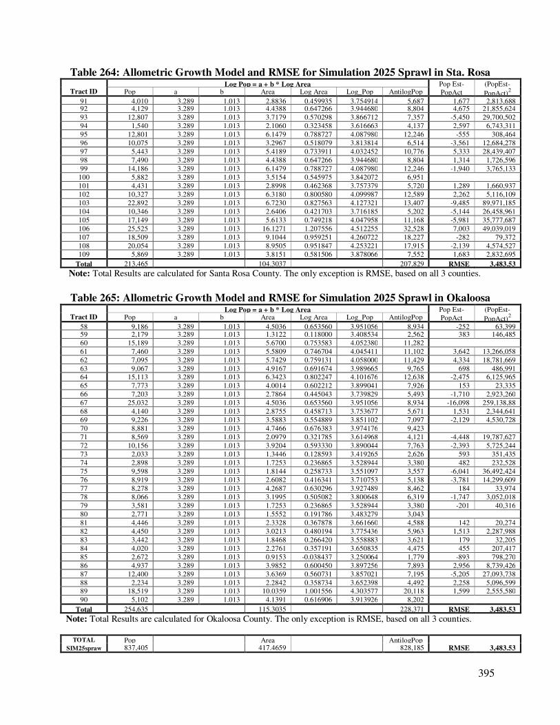
395
Table 264: Allometric Growth Model and RMSE for Simulation 2025 Sprawl in Sta. Rosa
Tract ID Log Pop = a + b * Log Area Pop Est-
PopAct
(PopEst-
PopAct)2 Pop a b Area Log Area Log_Pop AntilogPop
91 4,010 3.289 1.013 2.8836 0.459935 3.754914 5,687 1,677 2,813,688 92 4,129 3.289 1.013 4.4388 0.647266 3.944680 8,804 4,675 21,855,624
93 12,807 3.289 1.013 3.7179 0.570298 3.866712 7,357 -5,450 29,700,502
94 1,540 3.289 1.013 2.1060 0.323458 3.616663 4,137 2,597 6,743,311
95 12,801 3.289 1.013 6.1479 0.788727 4.087980 12,246 -555 308,464
96 10,075 3.289 1.013 3.2967 0.518079 3.813814 6,514 -3,561 12,684,278
97 5,443 3.289 1.013 5.4189 0.733911 4.032452 10,776 5,333 28,439,407
98 7,490 3.289 1.013 4.4388 0.647266 3.944680 8,804 1,314 1,726,596
99 14,186 3.289 1.013 6.1479 0.788727 4.087980 12,246 -1,940 3,765,133
100 5,882 3.289 1.013 3.5154 0.545975 3.842072 6,951
101 4,431 3.289 1.013 2.8998 0.462368 3.757379 5,720 1,289 1,660,937
102 10,327 3.289 1.013 6.3180 0.800580 4.099987 12,589 2,262 5,116,109
103 22,892 3.289 1.013 6.7230 0.827563 4.127321 13,407 -9,485 89,971,185
104 10,346 3.289 1.013 2.6406 0.421703 3.716185 5,202 -5,144 26,458,961
105 17,149 3.289 1.013 5.6133 0.749218 4.047958 11,168 -5,981 35,777,687
106 25,525 3.289 1.013 16.1271 1.207556 4.512255 32,528 7,003 49,039,019
107 18,509 3.289 1.013 9.1044 0.959251 4.260722 18,227 -282 79,372
108 20,054 3.289 1.013 8.9505 0.951847 4.253221 17,915 -2,139 4,574,527
109 5,869 3.289 1.013 3.8151 0.581506 3.878066 7,552 1,683 2,832,695
Total 213,465 104.3037 207,829 RMSE 3,483.53
Note: Total Results are calculated for Santa Rosa County. The only exception is RMSE, based on all 3 counties.
Table 265: Allometric Growth Model and RMSE for Simulation 2025 Sprawl in Okaloosa
Tract ID Log Pop = a + b * Log Area Pop Est-
PopAct
(PopEst-
PopAct)2 Pop a b Area Log Area Log_Pop AntilogPop
58 9,186 3.289 1.013 4.5036 0.653560 3.951056 8,934 -252 63,399 59 2,179 3.289 1.013 1.3122 0.118000 3.408534 2,562 383 146,485
60 15,189 3.289 1.013 5.6700 0.753583 4.052380 11,282
61 7,460 3.289 1.013 5.5809 0.746704 4.045411 11,102 3,642 13,266,058
62 7,095 3.289 1.013 5.7429 0.759131 4.058000 11,429 4,334 18,781,669
63 9,067 3.289 1.013 4.9167 0.691674 3.989665 9,765 698 486,991
64 15,113 3.289 1.013 6.3423 0.802247 4.101676 12,638 -2,475 6,125,965
65 7,773 3.289 1.013 4.0014 0.602212 3.899041 7,926 153 23,335
66 7,203 3.289 1.013 2.7864 0.445043 3.739829 5,493 -1,710 2,923,260
67 25,032 3.289 1.013 4.5036 0.653560 3.951056 8,934 -16,098 259,138,88
68 4,140 3.289 1.013 2.8755 0.458713 3.753677 5,671 1,531 2,344,641
69 9,226 3.289 1.013 3.5883 0.554889 3.851102 7,097 -2,129 4,530,728
70 8,881 3.289 1.013 4.7466 0.676383 3.974176 9,423
71 8,569 3.289 1.013 2.0979 0.321785 3.614968 4,121 -4,448 19,787,627
72 10,156 3.289 1.013 3.9204 0.593330 3.890044 7,763 -2,393 5,725,244
73 2,033 3.289 1.013 1.3446 0.128593 3.419265 2,626 593 351,435
74 2,898 3.289 1.013 1.7253 0.236865 3.528944 3,380 482 232,528
75 9,598 3.289 1.013 1.8144 0.258733 3.551097 3,557 -6,041 36,492,424
76 8,919 3.289 1.013 2.6082 0.416341 3.710753 5,138 -3,781 14,299,609
77 8,278 3.289 1.013 4.2687 0.630296 3.927489 8,462 184 33,974
78 8,066 3.289 1.013 3.1995 0.505082 3.800648 6,319 -1,747 3,052,018
79 3,581 3.289 1.013 1.7253 0.236865 3.528944 3,380 -201 40,316
80 2,771 3.289 1.013 1.5552 0.191786 3.483279 3,043
81 4,446 3.289 1.013 2.3328 0.367878 3.661660 4,588 142 20,274
82 4,450 3.289 1.013 3.0213 0.480194 3.775436 5,963 1,513 2,287,988
83 3,442 3.289 1.013 1.8468 0.266420 3.558883 3,621 179 32,205
84 4,020 3.289 1.013 2.2761 0.357191 3.650835 4,475 455 207,417
85 2,672 3.289 1.013 0.9153 -0.038437 3.250064 1,779 -893 798,270
86 4,937 3.289 1.013 3.9852 0.600450 3.897256 7,893 2,956 8,739,426
87 12,400 3.289 1.013 3.6369 0.560731 3.857021 7,195 -5,205 27,093,738
88 2,234 3.289 1.013 2.2842 0.358734 3.652398 4,492 2,258 5,096,599
89 18,519 3.289 1.013 10.0359 1.001556 4.303577 20,118 1,599 2,555,580
90 5,102 3.289 1.013 4.1391 0.616906 3.913926 8,202
Total 254,635 115.3035 228,371 RMSE 3,483.53
Note: Total Results are calculated for Okaloosa County. The only exception is RMSE, based on all 3 counties.
TOTAL Pop
Area
AntilogPop SIM25spraw 837,405 417.4659 828,185 RMSE 3,483.53
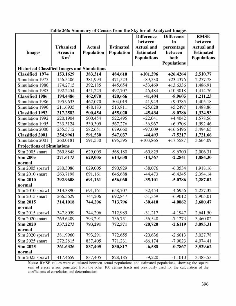
396
Table 266: Summary of Census from the Sky for all Analyzed Images
Images
Urbanized
Areas in
Km2
Actual
Population
Estimated
Population
Difference
between
Actual and
Estimated
Populations
Difference
in
percentage
between
both
Populations
RMSE
between
Actual and
Estimated
Populations
Historical Classified Images and Simulations
Classified 1974 153.1629 383,314 484,610 +101,296 +26.4264 2,510.77
Simulation 1975 156.5406 381,993 471,523 +89,530 +23.4376 2,277.78
Simulation 1980 174.2715 392,185 445,654 +53,469 +13.6336 1,486.91
Simulation 1985 192.2454 451,223 497,707 +46,484 +10.3018 1,414.76
Classified 1986 194.4486 462,070 420,666 -41,404 -8.9605 1,211.23
Simulation 1986 195.9633 462,070 504,019 +41,949 +9.0785 1,405.18
Simulation 1990 211.6935 488,183 513,811 +25,628 +5.2497 1,488.86
Classified 1992 217.2582 500,454 455,020 -45,434 -9.0786 1,324.93
Simulation 1992 220.1904 500,454 522,495 +22,041 +4.4042 1,578.56
Simulation 1995 233.3124 530,309 567,276 +36,967 +6.9708 1,992.46
Simulation 2000 255.5712 582,651 679,660 +97,009 +16.6496 3,494.65
Classified 2001 254.9961 591,530 547,037 -44,493 -7.5217 1,721.66
Simulation 2001 260.0181 591,530 695,395 +103,865 +17.5587 3,664.09
Projections of Simulations
Sim 2005 smart 260.8848 629,005 568,180 -60,825 -9.6700 2,006.31
Sim 2005
normal
271.6173 629,005 614,638 -14,367 -2.2841 1,884.30
Sim 2005 sprawl 280.3086 629,005 590,929 -38,076 -6.0534 1,918.16
Sim 2010 smart 263.7198 691,161 646,688 -44,473 -6.4345 2,394.14
Sim 2010
normal
292.9608 691,161 656,060 -35,101 -5.0786 2,287.02
Sim 2010 sprawl 313.3890 691,161 658,707 -32,454 -4.6956 2,257.32
Sim 2015 smart 266.5629 744,206 692,847 -51,359 -6.9012 2,905.01
Sim 2015
normal
314.1018 744,206 713,796 -30,410 -4.0862 2,680.47
Sim 2015 sprawl 347.8059 744,206 712,989 -31,217 -4.1947 2,641.50
Sim 2020 smart 269.6409 793,291 736,751 -56,540 -7.1273 3,460.02
Sim 2020
normal
337.2273 793,291 772,571 -20,720 -2.6119 3,095.31
Sim 2020 sprawl 381.9960 793,291 772,655 -20,636 -2.6013 3,027.78
Sim 2025 smart 272.2815 837,405 771,231 -66,174 -7.9023 4,074.41
Sim 2025
normal
361.6326 837,405 830,817 -6,588 -0.7867 3,529.62
Sim 2025 sprawl 417.4659 837,405 828,185 -9,220 -1.1010 3,483.53 Notes: RMSE values were calculated between actual populations and estimated populations, showing the square
sum of errors errors generated from the other 100 census tracts not previously used for the calculation of the coefficients of correlation and determination.
397
Analyzing this table is possible to notice that the higher the surface of the urban areas
(measured in Km2), the higher is also their populations, with the exceptions of the classified
Landsat images for years 1986, 1992 and 2001 with their respective simulations, because for
every one of these mentioned years, both have exactly the same population values at the census
tract level as well as in their total sums. The same happens with the simulations made from 2005
until 2025, because for every one of the selected years (2005, 2010, 1015, 2020 and 2025), the
smart growth, normal and urban sprawl trends have exactly the same population at the census
tract level and in their total sums, regardless of the amount of urbanized areas.
Also, it is very important to indicate that this table summarizes comparisons between actual
versus estimated populations, showing total differences in absolute and percentage values for the
whole population of every image in time, as well as for their Root Mean Square Errors (RMSE)
which implies differences at the census tract level. It is very interesting that results from future
simulations (2005 until 2025) show small differences between the total values of the actual
population in relation to the estimated population, while their total RMSE (measured at the
census tract level) indicates high levels of errors. The reason for this asymmetry is simply
because when the values of the estimated population at the census tract level are added together,
sometimes they are lower and sometimes they are higher than the ones from the actual
population, and by coincidence, at the end of the sum, the total value of the estimated population
can be similar to the one obtained from the sum of the actual population; therefore RMSE is
always the best measure to evaluate the accuracy of the census from the sky.
In addition, because population estimates depend on the amount of urbanized areas according
to the allometric growth model, and actual populations in the linear regression analyses made at
the beginning of this chapter constitute the dependent variable Y of urban areas (independent
variable X), it is possible to compare the differences in absolute and percentage values between
the total results of the estimated versus the actual populations for the whole region (Escambia,
Santa Rosa and Okaloosa counties) from table 266 against the correlation (R) and regression
coefficients (R2 and adjusted R
2) from table 153 (a linear regression of all 110 census tracts
between urban areas and actual populations). Doing this comparison, is possible to notice that in
some cases (especially with normal and urban sprawl simulations) the lower the regression
indexes are between urban areas and actual populations, the higher the differences are between
estimated and actual populations, and vice versa. The reason for these anomalies is the same
already explained: the coincidence at the end of the sum of adding sometimes lower and
sometimes higher estimated population values in relation to the total actual population.
Finally, this pattern sometimes does not occur between the Root Mean Square Errors (RMSE)
for the 100 census tracts and the measures obtained through linear regression analysis (with the
exceptions of classified and simulated images from 1980 to 1992); these results are totally
different and the lack of coincidence between the results of these two tables (correlation,
coefficient of determination in relation with RMSE) relates with the way how formulas were
designed to calculate these indexes, being enough to say that even if the measurement of values
from the cloud of points to the regression line is always the same, the calculation of these errors
varies according to the formulas used, becoming a whole new statistical topic beyond the area of
interest of this research. The pattern that is always present in the analysis of RMSE results is the
fact that the closer the simulations are from their origins (year 1974 for historical simulations and
year 2001 for future simulations), the lower are their RMSEs, and vice versa.
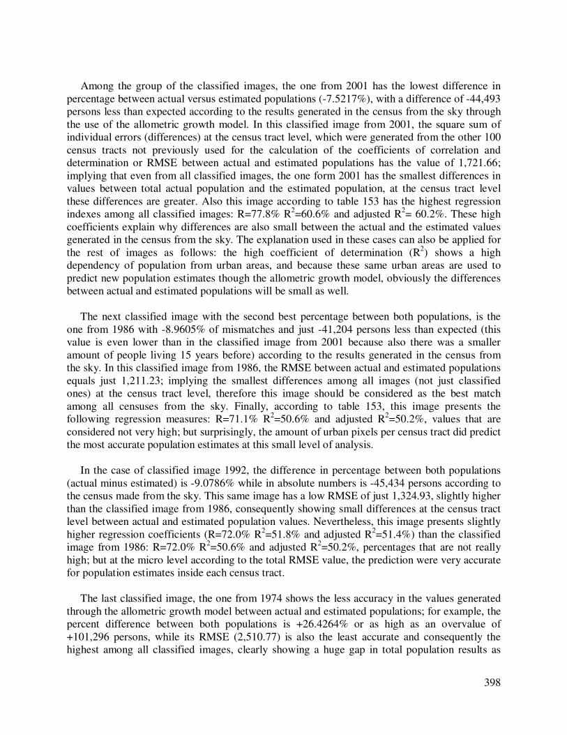
398
Among the group of the classified images, the one from 2001 has the lowest difference in
percentage between actual versus estimated populations (-7.5217%), with a difference of -44,493
persons less than expected according to the results generated in the census from the sky through
the use of the allometric growth model. In this classified image from 2001, the square sum of
individual errors (differences) at the census tract level, which were generated from the other 100
census tracts not previously used for the calculation of the coefficients of correlation and
determination or RMSE between actual and estimated populations has the value of 1,721.66;
implying that even from all classified images, the one form 2001 has the smallest differences in
values between total actual population and the estimated population, at the census tract level
these differences are greater. Also this image according to table 153 has the highest regression
indexes among all classified images: R=77.8% R2=60.6% and adjusted R
2= 60.2%. These high
coefficients explain why differences are also small between the actual and the estimated values
generated in the census from the sky. The explanation used in these cases can also be applied for
the rest of images as follows: the high coefficient of determination (R2) shows a high
dependency of population from urban areas, and because these same urban areas are used to
predict new population estimates though the allometric growth model, obviously the differences
between actual and estimated populations will be small as well.
The next classified image with the second best percentage between both populations, is the
one from 1986 with -8.9605% of mismatches and just -41,204 persons less than expected (this
value is even lower than in the classified image from 2001 because also there was a smaller
amount of people living 15 years before) according to the results generated in the census from
the sky. In this classified image from 1986, the RMSE between actual and estimated populations
equals just 1,211.23; implying the smallest differences among all images (not just classified
ones) at the census tract level, therefore this image should be considered as the best match
among all censuses from the sky. Finally, according to table 153, this image presents the
following regression measures: R=71.1% R2=50.6% and adjusted R
2=50.2%, values that are
considered not very high; but surprisingly, the amount of urban pixels per census tract did predict
the most accurate population estimates at this small level of analysis.
In the case of classified image 1992, the difference in percentage between both populations
(actual minus estimated) is -9.0786% while in absolute numbers is -45,434 persons according to
the census made from the sky. This same image has a low RMSE of just 1,324.93, slightly higher
than the classified image from 1986, consequently showing small differences at the census tract
level between actual and estimated population values. Nevertheless, this image presents slightly
higher regression coefficients (R=72.0% R2=51.8% and adjusted R
2=51.4%) than the classified
image from 1986: R=72.0% R2=50.6% and adjusted R
2=50.2%, percentages that are not really
high; but at the micro level according to the total RMSE value, the prediction were very accurate
for population estimates inside each census tract.
The last classified image, the one from 1974 shows the less accuracy in the values generated
through the allometric growth model between actual and estimated populations; for example, the
percent difference between both populations is +26.4264% or as high as an overvalue of
+101,296 persons, while its RMSE (2,510.77) is also the least accurate and consequently the
highest among all classified images, clearly showing a huge gap in total population results as
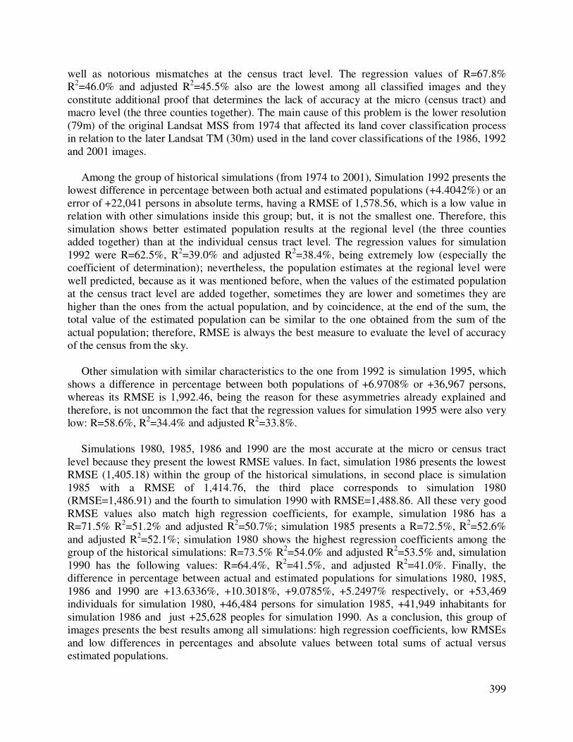
399
well as notorious mismatches at the census tract level. The regression values of R=67.8%
R2=46.0% and adjusted R
2=45.5% also are the lowest among all classified images and they
constitute additional proof that determines the lack of accuracy at the micro (census tract) and
macro level (the three counties together). The main cause of this problem is the lower resolution
(79m) of the original Landsat MSS from 1974 that affected its land cover classification process
in relation to the later Landsat TM (30m) used in the land cover classifications of the 1986, 1992
and 2001 images.
Among the group of historical simulations (from 1974 to 2001), Simulation 1992 presents the
lowest difference in percentage between both actual and estimated populations (+4.4042%) or an
error of +22,041 persons in absolute terms, having a RMSE of 1,578.56, which is a low value in
relation with other simulations inside this group; but, it is not the smallest one. Therefore, this
simulation shows better estimated population results at the regional level (the three counties
added together) than at the individual census tract level. The regression values for simulation
1992 were R=62.5%, R2=39.0% and adjusted R
2=38.4%, being extremely low (especially the
coefficient of determination); nevertheless, the population estimates at the regional level were
well predicted, because as it was mentioned before, when the values of the estimated population
at the census tract level are added together, sometimes they are lower and sometimes they are
higher than the ones from the actual population, and by coincidence, at the end of the sum, the
total value of the estimated population can be similar to the one obtained from the sum of the
actual population; therefore, RMSE is always the best measure to evaluate the level of accuracy
of the census from the sky.
Other simulation with similar characteristics to the one from 1992 is simulation 1995, which
shows a difference in percentage between both populations of +6.9708% or +36,967 persons,
whereas its RMSE is 1,992.46, being the reason for these asymmetries already explained and
therefore, is not uncommon the fact that the regression values for simulation 1995 were also very
low: R=58.6%, R2=34.4% and adjusted R
2=33.8%.
Simulations 1980, 1985, 1986 and 1990 are the most accurate at the micro or census tract
level because they present the lowest RMSE values. In fact, simulation 1986 presents the lowest
RMSE (1,405.18) within the group of the historical simulations, in second place is simulation
1985 with a RMSE of 1,414.76, the third place corresponds to simulation 1980
(RMSE=1,486.91) and the fourth to simulation 1990 with RMSE=1,488.86. All these very good
RMSE values also match high regression coefficients, for example, simulation 1986 has a
R=71.5% R2=51.2% and adjusted R
2=50.7%; simulation 1985 presents a R=72.5%, R
2=52.6%
and adjusted R2=52.1%; simulation 1980 shows the highest regression coefficients among the
group of the historical simulations: R=73.5% R2=54.0% and adjusted R
2=53.5% and, simulation
1990 has the following values: R=64.4%, R2=41.5%, and adjusted R
2=41.0%. Finally, the
difference in percentage between actual and estimated populations for simulations 1980, 1985,
1986 and 1990 are +13.6336%, +10.3018%, +9.0785%, +5.2497% respectively, or +53,469
individuals for simulation 1980, +46,484 persons for simulation 1985, +41,949 inhabitants for
simulation 1986 and just +25,628 peoples for simulation 1990. As a conclusion, this group of
images presents the best results among all simulations: high regression coefficients, low RMSEs
and low differences in percentages and absolute values between total sums of actual versus
estimated populations.
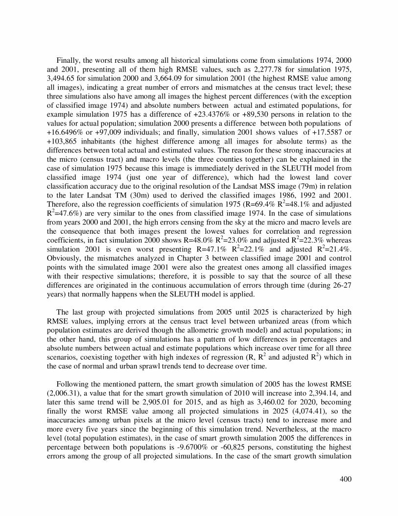
400
Finally, the worst results among all historical simulations come from simulations 1974, 2000
and 2001, presenting all of them high RMSE values, such as 2,277.78 for simulation 1975,
3,494.65 for simulation 2000 and 3,664.09 for simulation 2001 (the highest RMSE value among
all images), indicating a great number of errors and mismatches at the census tract level; these
three simulations also have among all images the highest percent differences (with the exception
of classified image 1974) and absolute numbers between actual and estimated populations, for
example simulation 1975 has a difference of +23.4376% or +89,530 persons in relation to the
values for actual population; simulation 2000 presents a difference between both populations of
+16.6496% or +97,009 individuals; and finally, simulation 2001 shows values of +17.5587 or
+103,865 inhabitants (the highest difference among all images for absolute terms) as the
differences between total actual and estimated values. The reason for these strong inaccuracies at
the micro (census tract) and macro levels (the three counties together) can be explained in the
case of simulation 1975 because this image is immediately derived in the SLEUTH model from
classified image 1974 (just one year of difference), which had the lowest land cover
classification accuracy due to the original resolution of the Landsat MSS image (79m) in relation
to the later Landsat TM (30m) used to derived the classified images 1986, 1992 and 2001.
Therefore, also the regression coefficients of simulation 1975 (R=69.4% R2=48.1% and adjusted
R2=47.6%) are very similar to the ones from classified image 1974. In the case of simulations
from years 2000 and 2001, the high errors censing from the sky at the micro and macro levels are
the consequence that both images present the lowest values for correlation and regression
coefficients, in fact simulation 2000 shows R=48.0% R2=23.0% and adjusted R
2=22.3% whereas
simulation 2001 is even worst presenting R=47.1% R2=22.1% and adjusted R
2=21.4%.
Obviously, the mismatches analyzed in Chapter 3 between classified image 2001 and control
points with the simulated image 2001 were also the greatest ones among all classified images
with their respective simulations; therefore, it is possible to say that the source of all these
differences are originated in the continuous accumulation of errors through time (during 26-27
years) that normally happens when the SLEUTH model is applied.
The last group with projected simulations from 2005 until 2025 is characterized by high
RMSE values, implying errors at the census tract level between urbanized areas (from which
population estimates are derived though the allometric growth model) and actual populations; in
the other hand, this group of simulations has a pattern of low differences in percentages and
absolute numbers between actual and estimate populations which increase over time for all three
scenarios, coexisting together with high indexes of regression (R, R2 and adjusted R
2) which in
the case of normal and urban sprawl trends tend to decrease over time.
Following the mentioned pattern, the smart growth simulation of 2005 has the lowest RMSE
(2,006.31), a value that for the smart growth simulation of 2010 will increase into 2,394.14, and
later this same trend will be 2,905.01 for 2015, and as high as 3,460.02 for 2020, becoming
finally the worst RMSE value among all projected simulations in 2025 (4,074.41), so the
inaccuracies among urban pixels at the micro level (census tracts) tend to increase more and
more every five years since the beginning of this simulation trend. Nevertheless, at the macro
level (total population estimates), in the case of smart growth simulation 2005 the differences in
percentage between both populations is -9.6700% or -60,825 persons, constituting the highest
errors among the group of all projected simulations. In the case of the smart growth simulation
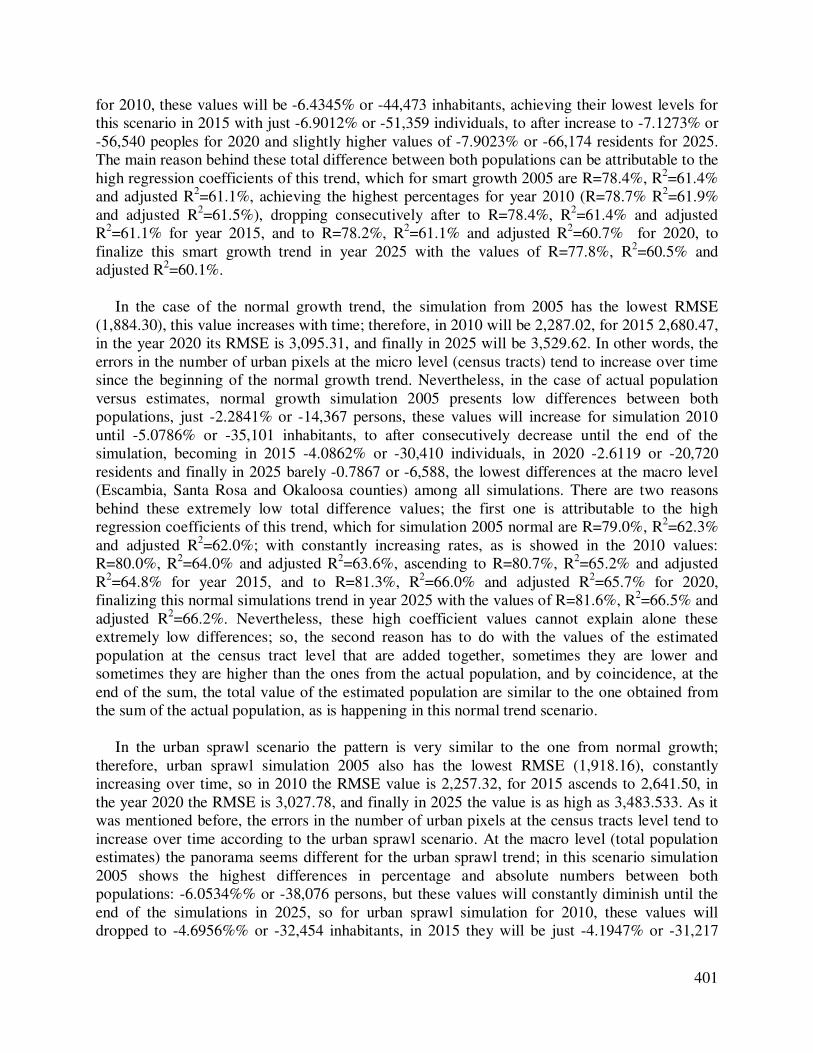
401
for 2010, these values will be -6.4345% or -44,473 inhabitants, achieving their lowest levels for
this scenario in 2015 with just -6.9012% or -51,359 individuals, to after increase to -7.1273% or
-56,540 peoples for 2020 and slightly higher values of -7.9023% or -66,174 residents for 2025.
The main reason behind these total difference between both populations can be attributable to the
high regression coefficients of this trend, which for smart growth 2005 are R=78.4%, R2=61.4%
and adjusted R2=61.1%, achieving the highest percentages for year 2010 (R=78.7% R
2=61.9%
and adjusted R2=61.5%), dropping consecutively after to R=78.4%, R
2=61.4% and adjusted
R2=61.1% for year 2015, and to R=78.2%, R
2=61.1% and adjusted R
2=60.7% for 2020, to
finalize this smart growth trend in year 2025 with the values of R=77.8%, R2=60.5% and
adjusted R2=60.1%.
In the case of the normal growth trend, the simulation from 2005 has the lowest RMSE
(1,884.30), this value increases with time; therefore, in 2010 will be 2,287.02, for 2015 2,680.47,
in the year 2020 its RMSE is 3,095.31, and finally in 2025 will be 3,529.62. In other words, the
errors in the number of urban pixels at the micro level (census tracts) tend to increase over time
since the beginning of the normal growth trend. Nevertheless, in the case of actual population
versus estimates, normal growth simulation 2005 presents low differences between both
populations, just -2.2841% or -14,367 persons, these values will increase for simulation 2010
until -5.0786% or -35,101 inhabitants, to after consecutively decrease until the end of the
simulation, becoming in 2015 -4.0862% or -30,410 individuals, in 2020 -2.6119 or -20,720
residents and finally in 2025 barely -0.7867 or -6,588, the lowest differences at the macro level
(Escambia, Santa Rosa and Okaloosa counties) among all simulations. There are two reasons
behind these extremely low total difference values; the first one is attributable to the high
regression coefficients of this trend, which for simulation 2005 normal are R=79.0%, R2=62.3%
and adjusted R2=62.0%; with constantly increasing rates, as is showed in the 2010 values:
R=80.0%, R2=64.0% and adjusted R
2=63.6%, ascending to R=80.7%, R
2=65.2% and adjusted
R2=64.8% for year 2015, and to R=81.3%, R
2=66.0% and adjusted R
2=65.7% for 2020,
finalizing this normal simulations trend in year 2025 with the values of R=81.6%, R2=66.5% and
adjusted R2=66.2%. Nevertheless, these high coefficient values cannot explain alone these
extremely low differences; so, the second reason has to do with the values of the estimated
population at the census tract level that are added together, sometimes they are lower and
sometimes they are higher than the ones from the actual population, and by coincidence, at the
end of the sum, the total value of the estimated population are similar to the one obtained from
the sum of the actual population, as is happening in this normal trend scenario.
In the urban sprawl scenario the pattern is very similar to the one from normal growth;
therefore, urban sprawl simulation 2005 also has the lowest RMSE (1,918.16), constantly
increasing over time, so in 2010 the RMSE value is 2,257.32, for 2015 ascends to 2,641.50, in
the year 2020 the RMSE is 3,027.78, and finally in 2025 the value is as high as 3,483.533. As it
was mentioned before, the errors in the number of urban pixels at the census tracts level tend to
increase over time according to the urban sprawl scenario. At the macro level (total population
estimates) the panorama seems different for the urban sprawl trend; in this scenario simulation
2005 shows the highest differences in percentage and absolute numbers between both
populations: -6.0534%% or -38,076 persons, but these values will constantly diminish until the
end of the simulations in 2025, so for urban sprawl simulation for 2010, these values will
dropped to -4.6956%% or -32,454 inhabitants, in 2015 they will be just -4.1947% or -31,217
402
individuals, decreasing to -2.6013% or -20,636 peoples for 2020 and to just -1.1010% or -9,220
residents for 2025. The main reason behind these total differences are the same already
mentioned for the case of the normal trend simulations. The first one, related with high
regression coefficients shows the following values for urban sprawl 2005: R=78.9%, R2=62.3%
and adjusted R2=62.0%, increasing to R=80.5%, R
2=64.8% and adjusted R
2=64.5% in year 2010,
after to R=81.3%, R2=66.1% and adjusted R
2=65.8% for 2015, ascending to R=82.2%,
R2=67.6% and adjusted R
2=67.3% for 2020, to finalize this urban sprawl trend in 2025 with the
values of R=82.4%, R2=68.0% and adjusted R
2=67.7%. But, of course, these differences among
total actual and estimated populations are very low to be explained just by the high regression
coefficients, so the second reason is related to the fact that positive and negative values added
together sometimes by coincidence, can achieve a total value for the estimated population similar
to the sum of the actual population, as is happening in this urban sprawl scenario.
Related Documents