Chapter 5 Theory and Design of Soundfield Reproduction 5.1 Introduction A problem relevant to emerging surround sound technology is the accurate repro- duction of a soundfield over a region of space. Using a set of loudspeakers, it is possible for listeners to spatialize sound and fully experience what it is actually like to be in the original sound environment. Soundfield reproduction has been discussed since the 1960s. However much of the work does not directly address soundfield reproduction in reverberant environments. In this chapter, using an efficient parametrization of the room transfer function we extend soundfield repro- duction to reverberant enclosures. Early work in soundfield reproduction was performed by Gerzon [32]. With his ambisonics system, Gerzon reproduced the first order spherical harmonics of a plane wave soundfield around a point in space. Ambisonics has since been unified with holography [74, 75], both of which rely on the Kirchoff-Helmholtz equation. Here, soundfield reproduction inside a control region is achieved by controlling the sound pressure and its normal derivative over the boundary of the control region [8]. In similar work, global soundfield reproduction techniques [46, 97] have been proposed which control sound pressure over the boundary. By controlling sound at additional points inside the control region, these techniques obviate the need for velocity microphones. Unfortunately, such techniques require a large number of loudspeakers. For lesser numbers of loudspeakers, least squares techniques have been suggested by Kirkeby et al. [52, 54]. Recently, using a spherical harmonic analysis, the theoretical minimum number of loudspeakers required for accurate reproduction of a plane wave has been established [106]. The reverberant case is made difficult by the rapid variation of the acoustic transfer functions over the room [68]. The standard approach has been to equalize the transfer functions over multiple points using least squares techniques [53,72]. 103

Welcome message from author
This document is posted to help you gain knowledge. Please leave a comment to let me know what you think about it! Share it to your friends and learn new things together.
Transcript
Chapter 5
Theory and Design of Soundfield
Reproduction
5.1 Introduction
A problem relevant to emerging surround sound technology is the accurate repro-
duction of a soundfield over a region of space. Using a set of loudspeakers, it is
possible for listeners to spatialize sound and fully experience what it is actually
like to be in the original sound environment. Soundfield reproduction has been
discussed since the 1960s. However much of the work does not directly address
soundfield reproduction in reverberant environments. In this chapter, using an
efficient parametrization of the room transfer function we extend soundfield repro-
duction to reverberant enclosures.
Early work in soundfield reproduction was performed by Gerzon [32]. With
his ambisonics system, Gerzon reproduced the first order spherical harmonics of a
plane wave soundfield around a point in space. Ambisonics has since been unified
with holography [74, 75], both of which rely on the Kirchoff-Helmholtz equation.
Here, soundfield reproduction inside a control region is achieved by controlling the
sound pressure and its normal derivative over the boundary of the control region
[8]. In similar work, global soundfield reproduction techniques [46, 97] have been
proposed which control sound pressure over the boundary. By controlling sound
at additional points inside the control region, these techniques obviate the need
for velocity microphones. Unfortunately, such techniques require a large number
of loudspeakers. For lesser numbers of loudspeakers, least squares techniques have
been suggested by Kirkeby et al. [52, 54]. Recently, using a spherical harmonic
analysis, the theoretical minimum number of loudspeakers required for accurate
reproduction of a plane wave has been established [106].
The reverberant case is made difficult by the rapid variation of the acoustic
transfer functions over the room [68]. The standard approach has been to equalize
the transfer functions over multiple points using least squares techniques [53, 72].
103

104 Theory and Design of Soundfield Reproduction
However equalization away from the design points is poor. In contrast soundfield
reproduction would require the equalization to extend over the whole control region.
Alternatively the acoustic transfer functions can be measured and incorporated
into the soundfield reproduction algorithm directly. Methods for estimating the
acoustic transfer functions over a region have been established by Mourjopou-
los [69] and Bharitkar and Kyriakakis [9], which sample the field at a number
of points and use a spatial equalization library. However these techniques do not
determine transfer functions with the accuracy required for soundfield reproduction
in a reverberant room.
In this chapter, we present a method of performing soundfield reproduction in
a reverberant room. This method is based on an efficient parametrization of the
acoustic transfer function. We show that the acoustic transfer function can be
written as a weighted sum of the modes of the control region using a small num-
ber of terms. Using this parametrization, we reconstruct a soundfield accurately
over the whole control region. This approach exploits the standing wave structure
of the reverberant field generated by each loudspeaker to reproduce the desired
soundfield. We also describe a practical method for determining the active modes
of the acoustic transfer function between each loudspeaker and the control region,
by sampling sound pressure at a small number of points.
This chapter is structured as follows. Section 5.2 casts soundfield reproduction
into a least squares framework, using the modal approach to gain insight into the
fundamental parameters of the problem. In particular we use the number of modes
active in the control region to estimate the required number of speakers. In Section
5.3, we describe a method for measuring the acoustic transfer functions from each
speaker to any point within the control region. This method hinges on a modal
parametrization of the acoustic transfer function. In this section we show how to
determine the modal parameters of the acoustic transfer function. We also analyze
the effect of noisy pressure samples on determining the modal parameters (Section
5.3.3). In Section 5.4 we extend the algorithm to the three dimensional case.
Section 5.5 demonstrates the performance of our soundfield reproduction technique
with several examples. Finally Section 5.6 discusses practical implementation.
5.2 Sound Field Reproduction
In this section, we devise a scheme of performing 2-D soundfield reproduction within
a reverberant enclosure. This 2-D technique ensures good reproduction in the
plane of the loudspeakers, provided each loudspeaker possesses a sizeable vertical
dimension. It is applicable to enclosures with highly sound-absorbing floors and
5.2 Sound Field Reproduction 105
G2(ω)
G`(ω)
B2
x
G1(ω)
GL(ω)
H`(x; ω)
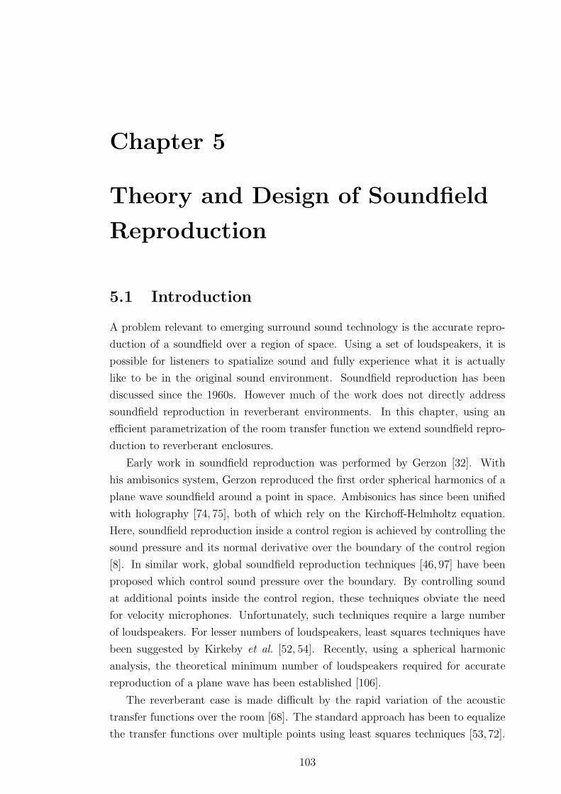
Figure 5.1: Use of L loudspeakers to reproduce a desired field in a control regionB2 with loudspeaker filters G`(ω) and acoustical transfer functions H`(x, ω) fromthe `th loudspeaker to a point x ∈ B2.
ceilings1.
The theory we develop here is extended to 3-D space in Section 5.4. This
extension entails replacing the 2-D modal functions described below with the 3-D
equivalent functions. However for accurate reproduction much larger numbers of
speakers are required [106]. We focus most attention on the 2-D case as it is more
practical.
Below we formulate the problem in the frequency domain. The objective is to
determine the loudspeaker filter weights required to reproduce a desired soundfield
in a reverberant room.
5.2.1 Problem Definition
We aim to reproduce the pressure Pd(x; ω) of a desired soundfield2 at each point
x and angular frequency ω in the source-free region of interest B2 using an array
of L loudspeakers. The desired soundfield could be a plane wave, a field resulting
from a monopole, a field measured in a real-life scenario or the field of a surround
sound system. For purposes of simplifying analysis in this chapter, we choose the
control region B2 to be the circle of radius R centered about origin:
B2 = {x ∈ R2 : ‖x‖ ≤ R}.
As shown in Figure 5.1, each loudspeaker ` transmits an output signal G`(ω).
1Due to the common use of carpet on the floors and foam spacers on the ceilings, both strongabsorbers of sound, such conditions hold in a large number of rooms.
2In contrast to all other chapters of this thesis, here a subscripted or superscripted d refer tothe desired soundfield and not the direct field component.

106 Theory and Design of Soundfield Reproduction
This signal encapsulates both the input signal applied to loudspeaker ` as well as
any filtering of it. To characterize the acoustic properties of the enclosure, define
the acoustic transfer function H`(x; ω). Each acoustic transfer function is the
frequency response between loudspeaker ` and point x. It describes the soundfield
due to a source and its reverberant reflections from the surface of the enclosure,
when a unit input signal G`(ω) ≡ 1 is applied to the source. The sound pressure
at any point x due to loudspeaker ` is equal to:
P`(x; ω) = G`(ω)H`(x; ω). (5.1)
From Figure 5.1, the sound pressure in the reproduced field resulting from the L
loudspeakers is then equal to
P (x; ω) =L∑
`=1
P`(x; ω) =L∑
`=1
G`(ω)H`(x; ω). (5.2)
The design task of soundfield reproduction is to choose filter weights G`(ω) to
minimize the normalized reproduction error J over B2,
J =1
E∫
B2
|P (x; ω)− Pd(x; ω)|2da(x) (5.3)
where the normalizing factor E is the energy of the desired soundfield over B2:
E =
∫
B2
|Pd(x; ω)|2da(x), (5.4)
da(x) = x dx dφx is the differential area element at x, x = ‖x‖ and φx is the polar
angle of x.
The popular approach to solving this problem is to write the least squares
solution over a set of uniformly-spaced points in B2 [52, 54]. A better approach is
to perform the design over the whole region. This approach is proposed by Asano
and Swason [5] for the related problem of equalization. Yet by discretizing, these
authors end up implementing a multi-point method. Below we outline a modal space
approach, which utilizes an efficient parametrization of acoustic transfer functions,
to perform the design over the whole region3. More insight is gained into the filter
design procedure through the modal space approach than through multi-point least
squares techniques.
3The modal space approach contrasts with the modal approaches of Asano and Swason [5]and Santillan [81], which only investigate equalization for rectangular room geometry.
5.2 Sound Field Reproduction 107
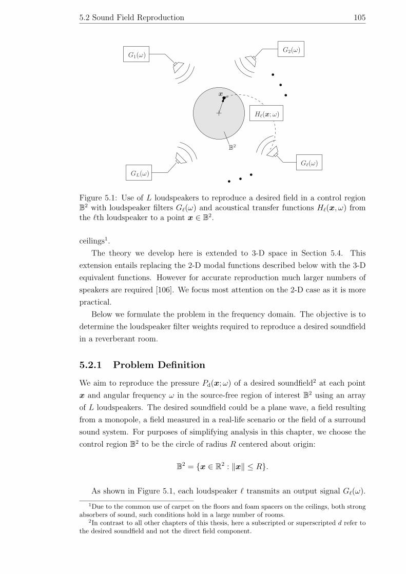
5.2.2 Modal Space Approach
In the modal space approach, we express the sound pressure variables Pd(x; ω),
P (x; ω) and the acoustic transfer functions H`(x; ω) in terms of the modes of
the soundfield. Provided all sound sources (including image-sources produced by
reflection) lie outside of B2, at any point inside B2 the above variables can be
written in modal form using the interior field solution (2.44) of Chapter 2. We
write the desired sound pressure Pd(x; ω) as:
Pd(x; ω) =∞∑
n=−∞β(d)
n (ω)Jn(kx)einφx , (5.5)
where β(d)n (ω) is the nth order modal coefficient of the desired soundfield at fre-
quency ω. Reviewing, the functions {Jn(kx)einφx}n∈Z are called the modes of the
soundfield. Appropriate choice of modal coefficients generate any valid soundfield
inside B2.
Similarly, we write the reproduced sound pressure P (x; ω) as:
P (x; ω) =∞∑
n=−∞βn(ω)Jn(kx)einφx , (5.6)
where βn(ω) are the modal coefficients of the reproduced soundfield. Reproduction
of the sound pressure Pd(x; ω) over B2 with P (x; ω) is equivalent to reproduction
of the modal coefficients {β(d)n (ω)}n∈Z with {βn(ω)}n∈Z.
Because H`(x; ω) is equal to the soundfield pressure when the loudspeaker is
excited by a unit impulse, we can also write it in modal form as:
H`(x; ω) =∞∑
n=−∞αn(`, ω)Jn(kx)einφx , (5.7)
where αn(`, ω) are the modal coefficients of the room responses for loudspeaker `.
These modal coefficients completely characterize the reverberant soundfield gener-
ated by each loudspeaker within B2:
Observation 5.2.1 When the modal coefficients αn(`, ω) for each loudspeaker are
known for a given room environment, the room response H`(x; ω) between each
loudspeaker and any position x inside B2 is also known, and is given by (5.7).
Substituting (5.5) and (5.7) directly into (5.2), the modal coefficients of the
reproduced soundfield are related to αn(`, ω) through
βn(ω) =L∑
`=1
G`(ω)αn(`, ω). (5.8)
108 Theory and Design of Soundfield Reproduction
The sequences of coefficients (β(d)n (ω))n, (βn(ω))n and (αn(`, ω))n associated
with any wave field in a source-free region are shown to be bounded in Jones et
al. [48].
We now derive an expression for the energy E and normalized error J of the
reproduced soundfield over B2 as a function of the modal coefficients. Starting with
the field energy, we substitute (5.5) into (5.4) to yield:
E =
∫
B2
∣∣∣∣∣∞∑
n=−∞β(d)
n (ω)Jn(kx)einφx
∣∣∣∣∣
2
da(x).
It follows that:
E =∞∑
m=−∞
∞∑n=−∞
[β(d)m (ω)]∗β(d)
n (ω)
∫ 2π
0
e−imφxeinφxdφx
×∫ R
0
Jm(kx)Jn(kx)x dx,
where we have applied da(x) = x dx dφx. Applying the orthogonality property
(2.42), the field energy reduces to:
E = 2π∞∑
n=−∞|β(d)
n (ω)|2∫ R
0
[Jn(kx)]2x dx
=2π
k2
∞∑n=−∞
wn(kR)|β(d)n (ω)|2, (5.9)
where
wn(kR) , k2
∫ R
0
[Jn(kx)]2x dx
=
∫ kR
0
[Jn(x)]2xdx. (5.10)
The second step was performed with the variable substitution x′ = kx. Similarly
substituting (5.5) and (5.6) into (5.3), the normalized error becomes:
J =1
E∫
B2
∣∣∣∣∣∞∑
n=−∞[βn(ω)− β(d)
n (ω)]Jn(kx)einφx
∣∣∣∣∣
2
da(x).
Utilizing the orthogonality property, the normalized error reduces to:
J =2π
k2E∞∑
n=−∞wn(kR)|β(d)
n (ω)− βn(ω)|2. (5.11)
We shall call wn(kR) in (5.11) the modal coefficient weighting function.
Since the summations in (5.5), (5.6) and (5.7) have an infinite numbers of terms,
5.2 Sound Field Reproduction 109
it may seem that the soundfield or room response parametrization needs an infinite
number of coefficients. However in the next section, we show that for any finite
control region, the above parametrization needs only a finite number of coefficients
to accurately represent a soundfield or a room response.
5.2.3 Active Modes
Because of the high-pass character of Bessel functions, not all of the modes make
a significant energy contribution to the soundfield inside B2. Studying (5.11),
because the sequences of modal coefficients (β(d)n (ω))n and (βn(ω))n are bounded,
the energy contribution of each modal term to reproduction error is controlled by
wn(kR). The reason for domination by wn(kR) is that for fixed kR, wn(kR) drops
rapidly to zero as n is increased. To see this fact, consider the following upper
bound on Jn(x) derived by Jones et al. [48]:
|Jn(x)| ≤ 1√2πn
(ex
2n
)n
.
Substituting this upper bound into (5.42) and then performing the integration:
wn(kR) ≤∫ kR
0
1
2πn
(ex
2n
)2n
xdx
≤ 2n
2n + 1
(ekR
2n
)2n+2
.
Hence wn(kR) drops exponentially to zero past |n| > dekR/2e. The modes for
which |n| > ekR/2 make increasingly negligible contribution to the soundfield
energy inside B2.
Previous work [48, 106] asserts that only the modes of modal index up to
N = dkRe contribute significant energy to the soundfield inside B2. This result is
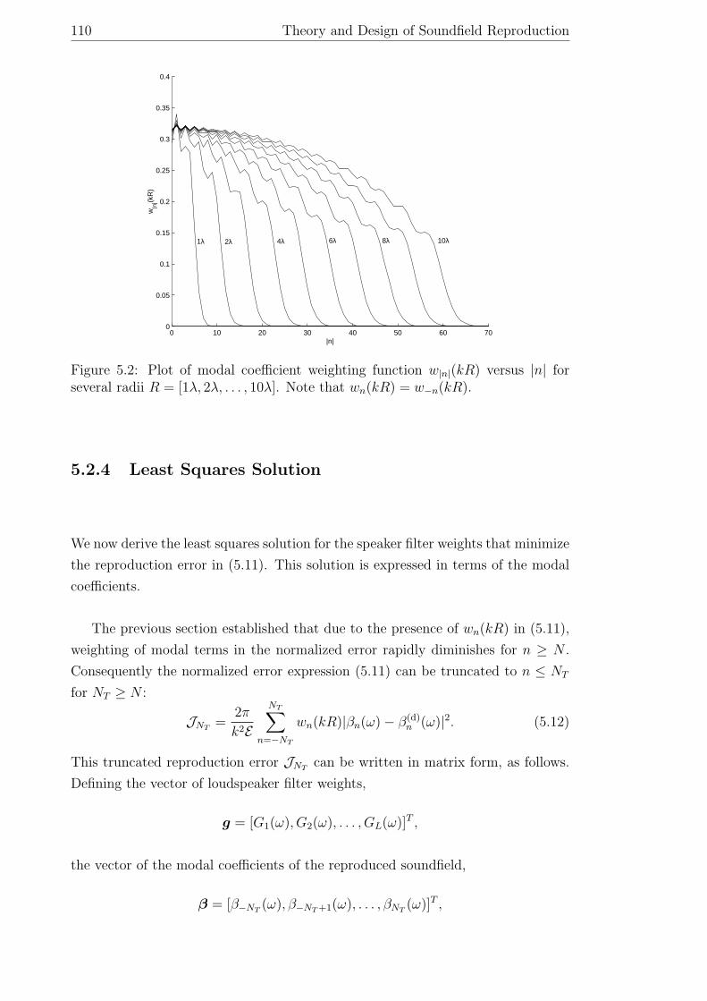
supported by Figure 5.2, where wn(kR) is plotted4 against n. The weighting is seen
to be small past |n| > N . The 2N + 1 modes, J−N(kx)e−iNφx , . . . , JN(kx) eiNφx
are referred to as the active modes of B2. The remaining modes are referred to as
inactive in B2. These modes make their contribution to the soundfield outside of
B2.
Accurate soundfield reproduction requires reproduction of these active modes.
Also, the room response between each loudspeaker and any points inside B2, as
mentioned in Observation 1, can be accurately determined just by measuring the
modal coefficients {αn(`, ω)}Nn=−N of the active modes.
4Note the weighting functions of the negative modal index are a mirror of those of the positivemodal index. This can be seen by applying the Bessel function property Jn(x) = (−1)nJ−n(x).
110 Theory and Design of Soundfield Reproduction
0 10 20 30 40 50 60 700
0.05
0.1
0.15
0.2
0.25
0.3
0.35
0.4
|n|
w|n
|(kR
)
2λ 4λ 6λ 8λ 10λ 1λ
Figure 5.2: Plot of modal coefficient weighting function w|n|(kR) versus |n| forseveral radii R = [1λ, 2λ, . . . , 10λ]. Note that wn(kR) = w−n(kR).
5.2.4 Least Squares Solution
We now derive the least squares solution for the speaker filter weights that minimize
the reproduction error in (5.11). This solution is expressed in terms of the modal
coefficients.
The previous section established that due to the presence of wn(kR) in (5.11),
weighting of modal terms in the normalized error rapidly diminishes for n ≥ N .
Consequently the normalized error expression (5.11) can be truncated to n ≤ NT
for NT ≥ N :
JNT=
2π
k2ENT∑
n=−NT
wn(kR)|βn(ω)− β(d)n (ω)|2. (5.12)
This truncated reproduction error JNTcan be written in matrix form, as follows.
Defining the vector of loudspeaker filter weights,
g = [G1(ω), G2(ω), . . . , GL(ω)]T ,
the vector of the modal coefficients of the reproduced soundfield,
β = [β−NT(ω), β−NT +1(ω), . . . , βNT
(ω)]T ,

5.2 Sound Field Reproduction 111
and the matrix of the modal coefficients of the room responses of all loudspeakers,
A =
α−NT(1, ω) α−NT
(2, ω) . . . α−NT(L, ω)
α1−NT(1, ω) α1−NT
(2, ω) . . . α1−NT(L, ω)
......
. . ....
αNT(1, ω) αNT
(2, ω) . . . αNT(L, ω)
, (5.13)
equation 5.8 can be rewritten as β = Ag. Additionally, define the vectors of the
modal coefficients of the desired soundfield,
βd = [β(d)−NT
(ω), β(d)−NT +1(ω), . . . , β
(d)NT
(ω)]T , (5.14)
and the diagonal weighting matrix,
W =
w−NT(kR) 0 . . . 0
0 w−NT +1(kR) . . . 0...
.... . .
...
0 0 . . . wNT(kR)
.
Writing the numerator of (5.12) in matrix form:
NT∑n=−NT
wn(kR)|βn(ω)− β(d)n (ω)|2 = (β − βd)
HW (β − βd),
the truncated reproduction error can be written as:
JNT=
(β − βd)HW (β − βd)
βHd Wβd
.
Since β = Ag, we expand the truncated reproduction error as a quadratic form in
the vector of loudspeaker filter weights:
JNT(g) =
1
d(gHBg − bHg − gHb + d),
where B = AHWA, b = AHWβd, d = βHd Wβd. From [5], this quadratic form
possesses it’s global minimum at:
g = B−1b = (AHWA)−1AHWβd, (5.15)
with the associated minimum in truncated reproduction error:
JNT(g) = 1− 1
dbHB−1b.
This modal space approach is superior to the conventional least squares approach
112 Theory and Design of Soundfield Reproduction
in that it ensures reproduction over the whole control region. It is also superior
to many previous techniques because it allows reproduction of any soundfield, not
just a plane wave. Further, once (AHWA)−1AHW is calculated for the acoustical
environment, the reproduced soundfield can be changed easily by modifying βd in
(5.15).
5.2.5 Mode-Matching Solution
As shown in Section 5.2.3, accurate soundfield reproduction is obtained by sim-
ply reproducing exactly the active modes of B2. In this reproduction strategy,
assuming non-degenerate speaker placement, only one loudspeaker is required to
reproduce each active modal coefficient (L = 2N + 1). Each active mode controls
the soundfield over a limited region of the space in B2.
For odd L, appropriate filter weights are chosen in order to set βn(ω) = β(d)n (ω)
for n = −(L− 1)/2,−(L− 1)/2 + 1, . . . , (L− 1)/2. Similar to the mode-matching
approach of [75], it requires solving the L× L linear system:
Ag = βd,
where A and βd are defined in (5.13) and (5.14) respectively here with NT =
(L − 1)/2. This solution is equivalent to a least squares solution with an equal
weighting matrix of low order modes, that is W = I2NT +1 where In is the n × n
identity matrix. Due to weighting the importance of different modes, the least
squares approach yields a slightly better reproduction performance. However, the
mode-matching approach is simpler.
The next section describes a method for measuring modal coefficients for the
acoustic transfer function in matrix A.
5.3 Estimation of Soundfield Coefficients
In this section we describe how to fully determine the soundfield inside a control
region B2 through measurement of the modal coefficients. This task is important
as it is required to calculate {αn(`, ω)}n∈Z that characterizes the reverberant field
generated by each loudspeaker.
We write the sound pressure P (x; ω) inside B2 generated by a loudspeaker
outside B2 in a reverberant enclosure as the modal expansion:
P (x; ω) =∞∑
n=−∞βn(ω)Jn(kx)einφx , (5.16)
where βn(ω) is the modal coefficient of order n. To determine the field pressure in-
5.3 Estimation of Soundfield Coefficients 113
βn
DFT(n) 1/Jn(kR)
R
(a)
R1
anDFT(n)
DFT(n) bn
R2
βn
(b)
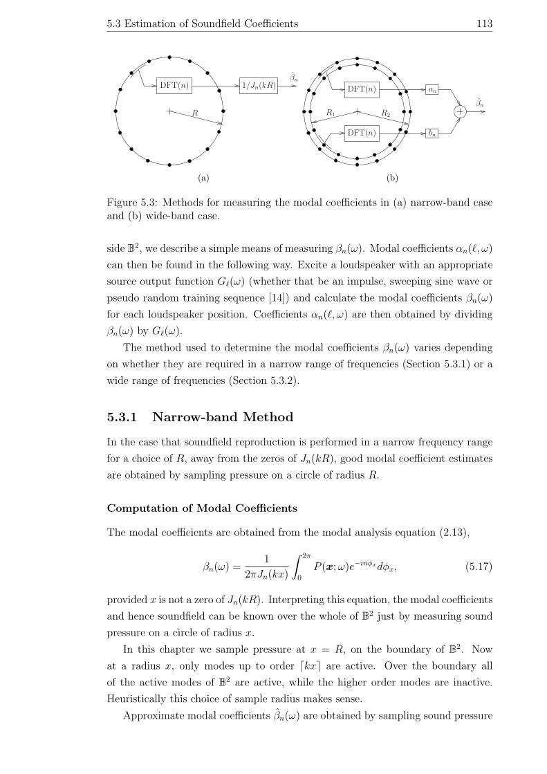
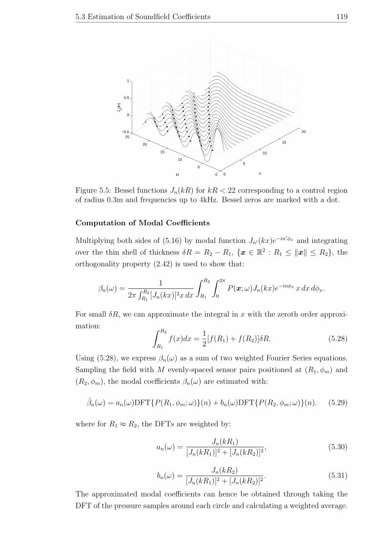
Figure 5.3: Methods for measuring the modal coefficients in (a) narrow-band caseand (b) wide-band case.
side B2, we describe a simple means of measuring βn(ω). Modal coefficients αn(`, ω)
can then be found in the following way. Excite a loudspeaker with an appropriate
source output function G`(ω) (whether that be an impulse, sweeping sine wave or
pseudo random training sequence [14]) and calculate the modal coefficients βn(ω)
for each loudspeaker position. Coefficients αn(`, ω) are then obtained by dividing
βn(ω) by G`(ω).
The method used to determine the modal coefficients βn(ω) varies depending
on whether they are required in a narrow range of frequencies (Section 5.3.1) or a
wide range of frequencies (Section 5.3.2).
5.3.1 Narrow-band Method
In the case that soundfield reproduction is performed in a narrow frequency range
for a choice of R, away from the zeros of Jn(kR), good modal coefficient estimates
are obtained by sampling pressure on a circle of radius R.
Computation of Modal Coefficients
The modal coefficients are obtained from the modal analysis equation (2.13),
βn(ω) =1
2πJn(kx)
∫ 2π
0
P (x; ω)e−inφxdφx, (5.17)
provided x is not a zero of Jn(kR). Interpreting this equation, the modal coefficients
and hence soundfield can be known over the whole of B2 just by measuring sound
pressure on a circle of radius x.
In this chapter we sample pressure at x = R, on the boundary of B2. Now
at a radius x, only modes up to order dkxe are active. Over the boundary all
of the active modes of B2 are active, while the higher order modes are inactive.
Heuristically this choice of sample radius makes sense.
Approximate modal coefficients βn(ω) are obtained by sampling sound pressure
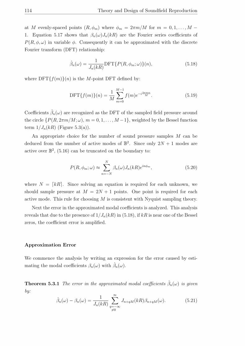
114 Theory and Design of Soundfield Reproduction
at M evenly-spaced points (R, φm) where φm = 2πm/M for m = 0, 1, . . . , M −1. Equation 5.17 shows that βn(ω)Jn(kR) are the Fourier series coefficients of
P (R, φ, ω) in variable φ. Consequently it can be approximated with the discrete
Fourier transform (DFT) relationship:
βn(ω) =1
Jn(kR)DFT{P (R, φm; ω)}(n), (5.18)
where DFT{f(m)}(n) is the M -point DFT defined by:
DFT{f(m)}(n) =1
M
M−1∑m=0
f(m)e−i 2πmnM . (5.19)
Coefficients βn(ω) are recognized as the DFT of the sampled field pressure around
the circle {P (R, 2πm/M ; ω), m = 0, 1, . . . , M−1}, weighted by the Bessel function
term 1/Jn(kR) (Figure 5.3(a)).
An appropriate choice for the number of sound pressure samples M can be
deduced from the number of active modes of B2. Since only 2N + 1 modes are
active over B2, (5.16) can be truncated on the boundary to:
P (R, φm; ω) ≈N∑
n=−N
βn(ω)Jn(kR)einφm , (5.20)
where N = dkRe. Since solving an equation is required for each unknown, we
should sample pressure at M = 2N + 1 points. One point is required for each
active mode. This rule for choosing M is consistent with Nyquist sampling theory.
Next the error in the approximated modal coefficients is analyzed. This analysis
reveals that due to the presence of 1/Jn(kR) in (5.18), if kR is near one of the Bessel
zeros, the coefficient error is amplified.
Approximation Error
We commence the analysis by writing an expression for the error caused by esti-
mating the modal coefficients βn(ω) with βn(ω).
Theorem 5.3.1 The error in the approximated modal coefficients βn(ω) is given
by:
βn(ω)− βn(ω) =1
Jn(kR)
∞∑q=−∞6=0
Jn+qM(kR)βn+qM(ω). (5.21)
5.3 Estimation of Soundfield Coefficients 115
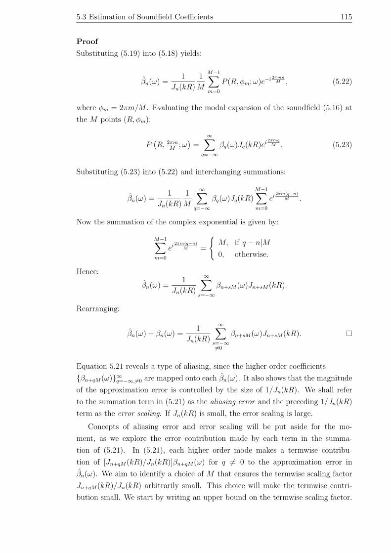
Proof
Substituting (5.19) into (5.18) yields:
βn(ω) =1
Jn(kR)
1
M
M−1∑m=0
P (R, φm; ω)e−i 2πmnM , (5.22)
where φm = 2πm/M . Evaluating the modal expansion of the soundfield (5.16) at
the M points (R, φm):
P(R, 2πm
M; ω
)=
∞∑q=−∞
βq(ω)Jq(kR)ei 2πmqM . (5.23)
Substituting (5.23) into (5.22) and interchanging summations:
βn(ω) =1
Jn(kR)
1
M
∞∑q=−∞
βq(ω)Jq(kR)M−1∑m=0
ei2πm(q−n)
M .
Now the summation of the complex exponential is given by:
M−1∑m=0
ei2πm(q−n)
M =
{M, if q − n|M0, otherwise.
Hence:
βn(ω) =1
Jn(kR)
∞∑s=−∞
βn+sM(ω)Jn+sM(kR).
Rearranging:
βn(ω)− βn(ω) =1
Jn(kR)
∞∑s=−∞6=0
βn+sM(ω)Jn+sM(kR).
Equation 5.21 reveals a type of aliasing, since the higher order coefficients
{βn+qM(ω)}∞q=−∞,6=0 are mapped onto each βn(ω). It also shows that the magnitude
of the approximation error is controlled by the size of 1/Jn(kR). We shall refer
to the summation term in (5.21) as the aliasing error and the preceding 1/Jn(kR)
term as the error scaling. If Jn(kR) is small, the error scaling is large.
Concepts of aliasing error and error scaling will be put aside for the mo-
ment, as we explore the error contribution made by each term in the summa-
tion of (5.21). In (5.21), each higher order mode makes a termwise contribu-
tion of [Jn+qM(kR)/Jn(kR)]βn+qM(ω) for q 6= 0 to the approximation error in
βn(ω). We aim to identify a choice of M that ensures the termwise scaling factor
Jn+qM(kR)/Jn(kR) arbitrarily small. This choice will make the termwise contri-
bution small. We start by writing an upper bound on the termwise scaling factor.
116 Theory and Design of Soundfield Reproduction
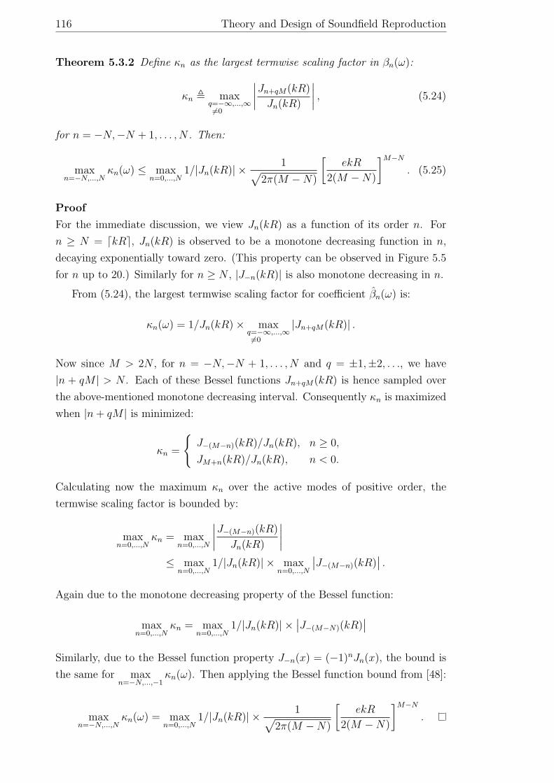
Theorem 5.3.2 Define κn as the largest termwise scaling factor in βn(ω):
κn , maxq=−∞,...,∞6=0
∣∣∣∣Jn+qM(kR)
Jn(kR)
∣∣∣∣ , (5.24)
for n = −N,−N + 1, . . . , N . Then:
maxn=−N,...,N
κn(ω) ≤ maxn=0,...,N
1/|Jn(kR)| × 1√2π(M −N)
[ekR
2(M −N)
]M−N
. (5.25)
Proof
For the immediate discussion, we view Jn(kR) as a function of its order n. For
n ≥ N = dkRe, Jn(kR) is observed to be a monotone decreasing function in n,
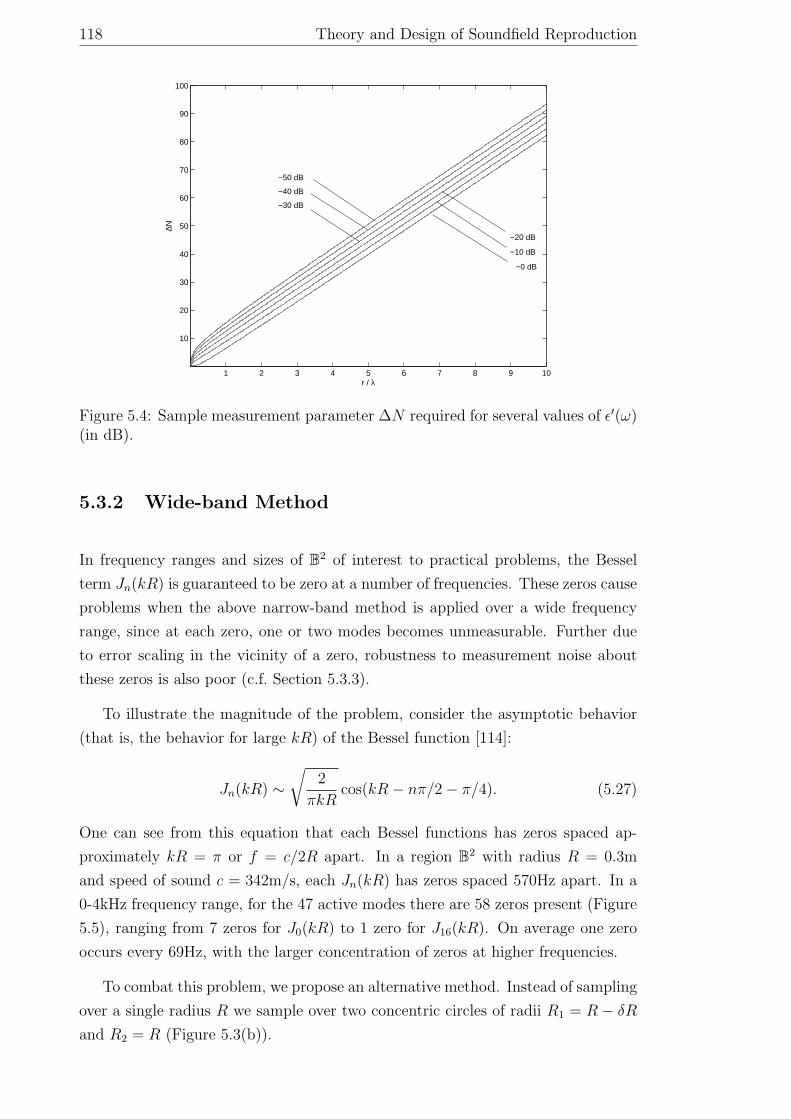
decaying exponentially toward zero. (This property can be observed in Figure 5.5
for n up to 20.) Similarly for n ≥ N , |J−n(kR)| is also monotone decreasing in n.
From (5.24), the largest termwise scaling factor for coefficient βn(ω) is:
κn(ω) = 1/Jn(kR)× maxq=−∞,...,∞6=0
|Jn+qM(kR)| .
Now since M > 2N , for n = −N,−N + 1, . . . , N and q = ±1,±2, . . ., we have
|n + qM | > N . Each of these Bessel functions Jn+qM(kR) is hence sampled over
the above-mentioned monotone decreasing interval. Consequently κn is maximized
when |n + qM | is minimized:
κn =
{J−(M−n)(kR)/Jn(kR), n ≥ 0,
JM+n(kR)/Jn(kR), n < 0.
Calculating now the maximum κn over the active modes of positive order, the
termwise scaling factor is bounded by:
maxn=0,...,N
κn = maxn=0,...,N
∣∣∣∣J−(M−n)(kR)
Jn(kR)
∣∣∣∣≤ max
n=0,...,N1/|Jn(kR)| × max
n=0,...,N
∣∣J−(M−n)(kR)∣∣ .
Again due to the monotone decreasing property of the Bessel function:
maxn=0,...,N
κn = maxn=0,...,N
1/|Jn(kR)| ×∣∣J−(M−N)(kR)
∣∣
Similarly, due to the Bessel function property J−n(x) = (−1)nJn(x), the bound is
the same for maxn=−N,...,−1
κn(ω). Then applying the Bessel function bound from [48]:
maxn=−N,...,N
κn(ω) = maxn=0,...,N
1/|Jn(kR)| × 1√2π(M −N)
[ekR
2(M −N)
]M−N
.
5.3 Estimation of Soundfield Coefficients 117
The first term of the upper bound in (5.25), maxn=0,...,N 1/|Jn(kR)|, is the maximum
error scaling and shall be denoted as κes(ω). The second term is an upper bound
on the Bessel function JM−N(kR) obtained from [48]. We note in (5.25) that the
largest termwise scaling factor decays exponentially to zero as M is increased past
N + dekR/2e. This observation suggests choosing M ≈ N + dekR/2e. Further the
bound on the termwise scaling factor motivates use of the following procedure for
the choice of M .
Conservative Estimate of M
We now describe a procedure that allows a more accurate choice of M than above:
a) Choose the desired bound ε on the termwise scaling factor; i.e. choose a bound
for which maxn=−N,...,N
κn(ω) < ε.
b) Calculate the maximum error scaling:
κes(ω) = maxn=0,1,...,N
|1/Jn(kR)|.
c) Determine ∆N = M −N through the relationship:
1√2π∆N
[ekR
2∆N
]∆N
= ε′(ω) (5.26)
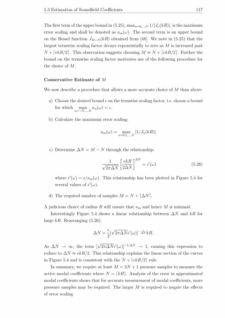
where ε′(ω) = ε/κes(ω). This relationship has been plotted in Figure 5.4 for
several values of ε′(ω).
d) The required number of samples M = N + d∆Ne.
A judicious choice of radius R will ensure that κes and hence M is minimal.
Interestingly Figure 5.4 shows a linear relationship between ∆N and kR for
large kR. Rearranging (5.26):
∆N =e
2[√
2π∆Nε′(ω)]−1
∆N kR.
As ∆N → ∞, the term [√
2π∆Nε′(ω)]−1/∆N → 1, causing this expression to
reduce to ∆N ≈ ekR/2. This relationship explains the linear section of the curves
in Figure 5.4 and is consistent with the N + dekR/2e rule.
In summary, we require at least M = 2N + 1 pressure samples to measure the
active modal coefficients where N = dkRe. Analysis of the error in approximated
modal coefficients shows that for accurate measurement of modal coefficients, more
pressure samples may be required. The larger M is required to negate the effects
of error scaling.
118 Theory and Design of Soundfield Reproduction
1 2 3 4 5 6 7 8 9 10
10
20
30
40
50
60
70
80
90
100
r / λ
∆N
−0 dB
−10 dB
−20 dB
−30 dB
−40 dB
−50 dB
Figure 5.4: Sample measurement parameter ∆N required for several values of ε′(ω)(in dB).
5.3.2 Wide-band Method
In frequency ranges and sizes of B2 of interest to practical problems, the Bessel
term Jn(kR) is guaranteed to be zero at a number of frequencies. These zeros cause
problems when the above narrow-band method is applied over a wide frequency
range, since at each zero, one or two modes becomes unmeasurable. Further due
to error scaling in the vicinity of a zero, robustness to measurement noise about
these zeros is also poor (c.f. Section 5.3.3).
To illustrate the magnitude of the problem, consider the asymptotic behavior
(that is, the behavior for large kR) of the Bessel function [114]:
Jn(kR) ∼√
2
πkRcos(kR− nπ/2− π/4). (5.27)
One can see from this equation that each Bessel functions has zeros spaced ap-
proximately kR = π or f = c/2R apart. In a region B2 with radius R = 0.3m
and speed of sound c = 342m/s, each Jn(kR) has zeros spaced 570Hz apart. In a
0-4kHz frequency range, for the 47 active modes there are 58 zeros present (Figure
5.5), ranging from 7 zeros for J0(kR) to 1 zero for J16(kR). On average one zero
occurs every 69Hz, with the larger concentration of zeros at higher frequencies.
To combat this problem, we propose an alternative method. Instead of sampling
over a single radius R we sample over two concentric circles of radii R1 = R − δR
and R2 = R (Figure 5.3(b)).
5.3 Estimation of Soundfield Coefficients 119
0
5
10
15
20
0
5
10
15
20
25−0.5
0
0.5
1
nkr
J n(kr)
Figure 5.5: Bessel functions Jn(kR) for kR < 22 corresponding to a control regionof radius 0.3m and frequencies up to 4kHz. Bessel zeros are marked with a dot.
Computation of Modal Coefficients
Multiplying both sides of (5.16) by modal function Jn′(kx)e−in′φx and integrating
over the thin shell of thickness δR = R2 − R1, {x ∈ R2 : R1 ≤ ‖x‖ ≤ R2}, the
orthogonality property (2.42) is used to show that:
βn(ω) =1
2π∫ R2
R1[Jn(kx)]2x dx
∫ R2
R1
∫ 2π
0
P (x; ω)Jn(kx)e−inφx x dx dφx.
For small δR, we can approximate the integral in x with the zeroth order approxi-
mation: ∫ R2
R1
f(x)dx =1
2[f(R1) + f(R2)]δR. (5.28)
Using (5.28), we express βn(ω) as a sum of two weighted Fourier Series equations.
Sampling the field with M evenly-spaced sensor pairs positioned at (R1, φm) and
(R2, φm), the modal coefficients βn(ω) are estimated with:
βn(ω) = an(ω)DFT{P (R1, φm; ω)}(n) + bn(ω)DFT{P (R2, φm; ω)}(n). (5.29)
where for R1 ≈ R2, the DFTs are weighted by:
an(ω) =Jn(kR1)
[Jn(kR1)]2 + [Jn(kR2)]2, (5.30)
bn(ω) =Jn(kR2)
[Jn(kR1)]2 + [Jn(kR2)]2. (5.31)
The approximated modal coefficients can hence be obtained through taking the
DFT of the pressure samples around each circle and calculating a weighted average.
120 Theory and Design of Soundfield Reproduction
Next we analyze the error in the approximated modal coefficients for the wide-
band case.
Approximation Error
For the wide-band method, the error in the approximated modal coefficients is:
βn(ω)− βn(ω) = an(ω) maxq=−∞,...,∞
q 6=0
Jn+qM(kR1)βn+qM(ω)
+ bn(ω)∞∑
q=−∞6=0
Jn+qM(kR2)βn+qM(ω). (5.32)
This expression is proven by substituting (5.19) into (5.29) and simplifying the
resulting expression in a manner similar to (5.21). In contrast to the narrow-band
case in (5.21), the wide-band case possesses two error scaling factors an(ω) and
bn(ω).
The presence of two Bessel functions Jn(kR1) and Jn(kR2) in the error scaling
factors (5.30) and (5.31) improves robustness at their zeros. They achieve the
improvement by weighting greater the pressure measurements from the radius at
which Jn(kR) is larger.
The critical parameter in the wide-band technique is δR. δR controls the maxi-
mum value of the error scaling terms an(ω) and bn(ω), as we will now show. When
either kR1 or kR2 is a zero of the Bessel function, approximation error simplifies to
that of the narrow-band case (5.21). For example, if Jn(kR1) = 0, the error scaling
terms reduce to an(ω) = 0 and bn(ω) = 1/|Jn(kR2)|. For δR small, Jn(kR2) is also
small and the linear approximation Jn(kR2) = kδRJ ′n(kR1) can be made. By the
derivative property of the Bessel function xJ ′n(x) = nJn(x)− xJn+1(x) [64, p. 24],
we see that J ′n(kR1) = Jn+1(kR1) so the nonzero error scaling term is
bn(ω) ≈ 1
kδR|Jn+1(kR1)| .
From this equation, it seems advantageous to choose δR large, as a larger δR
implies a smaller error scaling. However if δR is too large, error scaling will start
to increase. In the worse case Jn(kR2) coincides with another zero of the same
Bessel function. As these Bessel functions are regularly spaced, we can choose a
δR to avoid this case. From (5.27) the Bessel zeros of Jn(kR) are spaced π apart.
Because the extrema of the Bessel functions are approximately half way between
the zeros, set kδR < π/2 or δR < λ/4. An appropriate choice of δR is hence 1/4
of the smallest acoustic wavelength of interest.
5.3 Estimation of Soundfield Coefficients 121
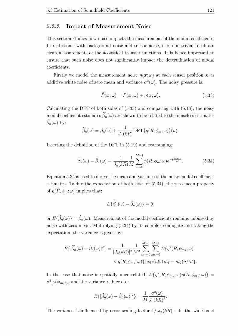
5.3.3 Impact of Measurement Noise
This section studies how noise impacts the measurement of the modal coefficients.
In real rooms with background noise and sensor noise, it is non-trivial to obtain
clean measurements of the acoustical transfer functions. It is hence important to
ensure that such noise does not significantly impact the determination of modal
coefficients.
Firstly we model the measurement noise η(x; ω) at each sensor position x as
additive white noise of zero mean and variance σ2(ω). The noisy pressure is:
P (x; ω) = P (x; ω) + η(x; ω). (5.33)
Calculating the DFT of both sides of (5.33) and comparing with (5.18), the noisy
modal coefficient estimates βn(ω) are shown to be related to the noiseless estimates
βn(ω) by:
βn(ω) = βn(ω) +1
Jn(kR)DFT{η(R, φm; ω)}(n).
Inserting the definition of the DFT in (5.19) and rearranging:
βn(ω)− βn(ω) =1
Jn(kR)
1
M
M−1∑m=0
η(R, φm; ω)e−i 2πmnM . (5.34)
Equation 5.34 is used to derive the mean and variance of the noisy modal coefficient
estimates. Taking the expectation of both sides of (5.34), the zero mean property
of η(R, φm; ω) implies that:
E{βn(ω)− βn(ω)} = 0,
or E{βn(ω)} = βn(ω). Measurement of the modal coefficients remains unbiased by
noise with zero mean. Multiplying (5.34) by its complex conjugate and taking the
expectation, the variance is given by:
E{|βn(ω)− βn(ω)|2} =1
[Jn(kR)]21
M2
M−1∑m1=0
M−1∑m2=0
E{η∗(R, φm1 ; ω)
× η(R, φm2 ; ω)} exp{i2π(m1 −m2)n/M}.
In the case that noise is spatially uncorrelated, E{η∗(R, φm1 ; ω)η(R, φm2 ; ω)} =
σ2(ω)δm1m2 and the variance reduces to:
E{|βn(ω)− βn(ω)|2} =1
M
σ2(ω)
Jn(kR)2 .
The variance is influenced by error scaling factor 1/|Jn(kR)|. In the wide-band
122 Theory and Design of Soundfield Reproduction
case, we can use a similar derivation to show that the modal coefficient estimates
are also unbiased and have a variance given by:
E{|βn(ω)− βn(ω)|2} =1
M
σ2(ω)
[Jn(kR1)]2 + [Jn(kR2)]2. (5.35)
The Bessel functions in the denominators of (5.35) show that similar error scaling
occurs in the noise error of the wide-band case. This error scaling has the potential
to greatly amplify the noise in measured modal coefficients if the Bessel functions
are small.
This error scaling of the noise also has implications on the measurability of the
inactive modal coefficients. For the inactive modes, the Bessel terms Jn(kR) are so
small as to be effectively zero. Thus error scaling in the inactive modes is so large
that the modal coefficients are unmeasurable.
5.4 Three Dimensional Case
We now extend the above theory to the reproduction of a soundfield in a volume
of space, by replacing the modal functions of the 2-D wave equation with the
analogous 3-D modal functions. A notable strength of this method is the ability
to reproduce the soundfield over the entire region of interest.
In Section 5.4.1 we define the soundfield reproduction problem in 3-D space and
in Section 5.4.2 we describe a method for determining the 3-D modal coefficients.
5.4.1 Sound Field Reproduction
We now show how to perform soundfield reproduction over a 3-D control region of
spherical shape. As for the 2-D case, our approach is to identify and reproduce the
active modes of the control region.
Problem Definition
The aim is to reproduce the sound pressure Pd(x; ω) of a desired field inside the
source-free region B3 = {x ∈ R3 : ‖x‖ ≤ R}. Each loudspeaker ` transmits the
output signal G`(ω) and possesses the acoustic transfer function H`(x; ω) between
the loudspeaker and each point in B3. The sound pressure P (x; ω) in the repro-
duced soundfield is again related to G`(ω) and H`(x; ω) for ` = 1, 2, . . . , L through
(5.1) and (5.2).
The design task of our 3-D soundfield reproduction is to choose filter weights
G`(ω) to minimize the normalized reproduction error J ,
J =1
E∫
B3
|P (x; ω)− Pd(x; ω)|2dv(x), (5.36)
5.4 Three Dimensional Case 123
where the energy of the desired soundfield E over B3 is:
E =
∫
B3
|Pd(x; ω)|2dv(x),
and dv(x) = x2 sin θx dx dθx dφx is the differential volume element at x and θx and
φx are the polar and azimuthal angles of x respectively. The next section describes
the modal approach of soundfield reproduction.
Modal Space Approach
In the modal space approach, the sound pressure variables Pd(x; ω) and P (x; ω)
and each acoustic transfer function H`(x; ω) are expressed in terms of the modes
of the soundfield. Applying the 3-D interior field solution (2.12) from Chapter 2,
within a source-free region these quantities are written as:
Pd(x; ω) =∞∑
n=0
n∑m=−n
β(d)nm(ω)jn(kx)Y m
n (x), (5.37)
P (x; ω) =∞∑
n=0
n∑m=−n
βnm(ω)jn(kx)Y mn (x), (5.38)
H`(x; ω) =∞∑
n=0
n∑m=−n
αnm(`, ω)jn(kx)Y mn (x), (5.39)
where β(d)nm(ω), βnm(ω) and αnm(`, ω) are the modal coefficients of the desired sound-
field, reproduced soundfield and acoustical transfer function for loudspeaker ` re-
spectively. Like in the 2-D case, soundfield reproduction can be performed by
reproduction of modal coefficients {β(d)nm(ω)} with {βnm(ω)}.
Similar to Observation 5.2.1, the modal coefficients αnm(`, ω) completely char-
acterize the acoustic transfer functions H`(x; ω) between each loudspeaker and any
position inside B3. Substituting (5.37) and (5.39) for H`(x; ω) into (5.2), the modal
coefficients of the reproduced soundfield are related to αnm(`, ω) through
βnm(ω) =L∑
`=1
G`(ω)αnm(`, ω). (5.40)
An expression for the energy E and normalized error J of the reproduced soundfield
over B3 as a function of the modal coefficients can be derived in a manner similar
to the 2-D case. The result is:
J =1
k3E∞∑
n=0
n∑m=−n
wn(kR)|βnm(ω)− β(d)nm(ω)|2, (5.41)

124 Theory and Design of Soundfield Reproduction
E =1
k3
∞∑n=0
n∑m=−n
wn(kR)|β(d)nm(ω)|2,
where the modal coefficient weighting function is given by:
wn(kR) =
∫ kR
0
[jn(x)]2x2dx. (5.42)
Next the activity properties of the modes in the 3-D case, are summarized.
Active Modes
Similar to the 2-D case, not all modes make a significant contribution to the field
inside the control region. Due to the low-pass property of the spherical Bessel
functions, some modes are active within B3 while others are inactive. In fact, Ward
and Abhayapala show that [106] as a rule of thumb only the modes {jn(kx)Y mn (x)}
for which n ≤ N = dkRe are active in the control region (just as in the 2-D case).
Once the coefficients of these modes are measured, the soundfield in B3 is accurately
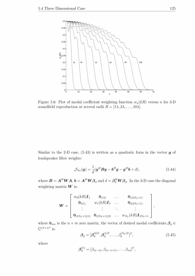
known. This property is observed in the plot of wn(kR) versus n in Figure 5.6.
The wn(kR) curves drop rapidly to zero past n = kR in a manner almost identical
that in the 2-D case (Figure 5.2).
The major difference in the 3-D case is that the number of active modes has
an approximate second order dependence on the frequency-radius product kR.
There are 2n + 1 active modes for each value of index n, creating∑N
n=0(2n + 1) =
(N+1)2 active modes instead of 2N+1. This dependence causes a large loudspeaker
requirement for accurate reproduction in moderately-sized control regions. For
example to reproduce the soundfield in a 1m diameter sphere we are required
to reconstruct 202 = 400 modes at 2kHz. For a practical limit on the number
of speakers, we must restrict 3-D reproduction to small control regions and low
frequencies.
Least Squares Solution
We now derive the least squares solution for the speaker weights that minimizes
(5.41). Because wn(kR) decays rapidly to zero for n > N = dkRe, while modal
coefficients {βnm(ω)} and {β(d)nm(ω)} are bounded in a similar sense to the 2-D case,
(5.41) is accurately truncated to NT for NT ≥ N :
JNT=
1
k3ENT∑n=0
n∑m=−n
wn(kR)|βnm(ω)− β(d)nm(ω)|2. (5.43)
5.4 Three Dimensional Case 125
0 10 20 30 40 50 60 700
0.05
0.1
0.15
0.2
0.25
0.3
0.35
0.4
0.45
0.5
n
wn(k
R)
2λ 4λ 6λ 8λ 10λ 1λ
Figure 5.6: Plot of modal coefficient weighting function wn(kR) versus n for 3-Dsoundfield reproduction at several radii R = [1λ, 2λ, . . . , 10λ].
Similar to the 2-D case, (5.43) is written as a quadratic form in the vector g of
loudspeaker filter weights:
JNT(g) =
1
d(gHBg − bHg − gHb + d), (5.44)
where B = AHWA, b = AHWβd and d = βHd Wβd. In the 3-D case the diagonal
weighting matrix W is:
W =
w0(kR)I1 01(3) . . . 01(2NT +1)
03(1) w1(kR)I3 . . . 03(2NT +1)
......
. . ....
0(2NT +1)(1) 0(2NT +1)(2) . . . wNT(kR)I2NT +1
,
where 0nm is the n×m zero matrix, the vector of desired modal coefficients βd ∈C(N+1)2 is:
βd = [β(0)Td ,β
(1)Td , . . . , β
(NT )Td ]T , (5.45)
where
β(n)d = [βn(−n), βn(−n+1), . . . , βnn]T ,
126 Theory and Design of Soundfield Reproduction
and the matrix of the modal coefficients of the room responses of all loudspeakers,
A =
α0(1, ω) α0(2, ω) . . . α0(L, ω)
α1(1, ω) α1(2, ω) . . . α1(L, ω)...
.... . .
...
αNT(1, ω) αNT
(2, ω) . . . αNT(L, ω)
,
where
αn(`, ω) = [αn(−n)(`, ω), αn(−n+1)(`, ω), . . . , αnn(`, ω)]T .
The least squares solution to (5.44) is again g = B−1b. This solution reproduces
the desired soundfield over the whole of B3.
Modal-Matching Solution
The mode-matching solution is identical in principle to the 2-D case. However at
least L = (N + 1)2 loudspeakers are required to match all the active modes of B3.
5.4.2 Estimation of 3-D Soundfield Coefficients
In this section, we devise a scheme for determining the modal coefficients of the
soundfield in the reproduction region. This task is extremely important to sound-
field reproduction in reverberant rooms. However, as will be seen below, it is of
limited practical interest because of the very large number of measurements needed.
Hence we limit treatment to the narrow-band case and only present a basic analy-
sis of the measurement error in the modal coefficients. Writing the sound pressure
P (x; ω) inside B3 generated by a loudspeaker outside as the modal expansion,
P (x; ω) =∞∑
n=0
n∑m=−n
βnm(ω)jn(kx)Y mn (x). (5.46)
where βnm(ω) are the modal coefficients of the soundfield that we desire to measure.
Computation of Modal Coefficients
The modal coefficients are obtained from the modal analysis equation (2.13) of
Chapter 2,
βnm(ω) =1
jn(kx)
∫
S2P (x; ω)[Y m
n (x)]∗ds(x), (5.47)
provided jn(kx) 6= 0. Sampling the pressure at M points Rφ1, Rφ2, . . . , RφM over
the boundary of B3, one can approximate the integral in (5.47) as:
βnm(ω) =1
jn(kR)
M∑t=1
P (Rφt; ω)[Y mn (φt)]
∗∆st, (5.48)
5.4 Three Dimensional Case 127
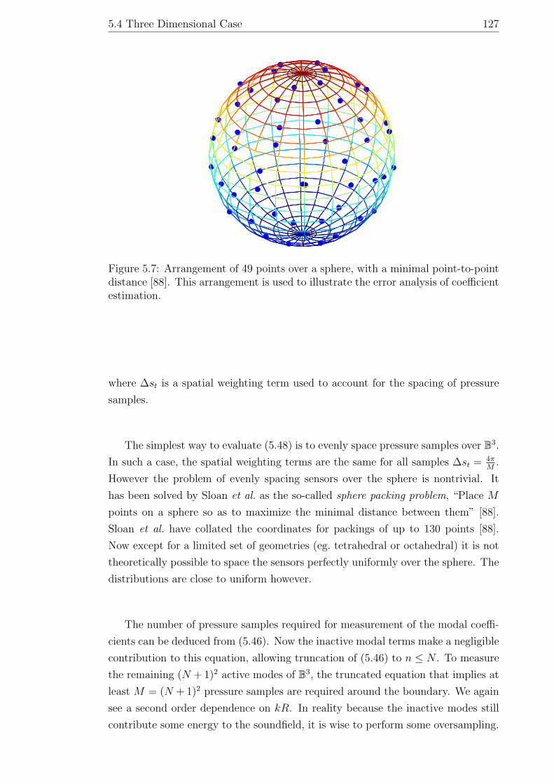
Figure 5.7: Arrangement of 49 points over a sphere, with a minimal point-to-pointdistance [88]. This arrangement is used to illustrate the error analysis of coefficientestimation.
where ∆st is a spatial weighting term used to account for the spacing of pressure
samples.
The simplest way to evaluate (5.48) is to evenly space pressure samples over B3.
In such a case, the spatial weighting terms are the same for all samples ∆st = 4πM
.
However the problem of evenly spacing sensors over the sphere is nontrivial. It
has been solved by Sloan et al. as the so-called sphere packing problem, “Place M
points on a sphere so as to maximize the minimal distance between them” [88].
Sloan et al. have collated the coordinates for packings of up to 130 points [88].
Now except for a limited set of geometries (eg. tetrahedral or octahedral) it is not
theoretically possible to space the sensors perfectly uniformly over the sphere. The
distributions are close to uniform however.
The number of pressure samples required for measurement of the modal coeffi-
cients can be deduced from (5.46). Now the inactive modal terms make a negligible
contribution to this equation, allowing truncation of (5.46) to n ≤ N . To measure
the remaining (N + 1)2 active modes of B3, the truncated equation that implies at
least M = (N + 1)2 pressure samples are required around the boundary. We again
see a second order dependence on kR. In reality because the inactive modes still
contribute some energy to the soundfield, it is wise to perform some oversampling.
128 Theory and Design of Soundfield Reproduction
0 20 40 60 80 100
0
50
100−40
−35
−30
−25
−20
−15
−10
−5
0
n‘q‘
10lo
g 10 δ
M(n
‘,q‘)
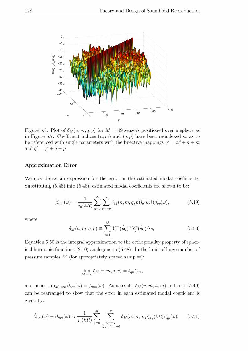
Figure 5.8: Plot of δM(n,m, q, p) for M = 49 sensors positioned over a sphere asin Figure 5.7. Coefficient indices (n,m) and (q, p) have been re-indexed so as tobe referenced with single parameters with the bijective mappings n′ = n2 + n + mand q′ = q2 + q + p.
Approximation Error
We now derive an expression for the error in the estimated modal coefficients.
Substituting (5.46) into (5.48), estimated modal coefficients are shown to be:
βnm(ω) =1
jn(kR)
∞∑q=0
q∑p=−q
δM(n,m, q, p)jq(kR)βqp(ω), (5.49)
where
δM(n,m, q, p) ,M∑t=1
[Y mn (φt)]
∗Y pq (φt)∆st. (5.50)
Equation 5.50 is the integral approximation to the orthogonality property of spher-
ical harmonic functions (2.10) analogous to (5.48). In the limit of large number of
pressure samples M (for appropriately spaced samples):
limM→∞
δM(n, m, q, p) = δqnδpm,
and hence limM→∞ βnm(ω) = βnm(ω). As a result, δM(n, m, n, m) ≈ 1 and (5.49)
can be rearranged to show that the error in each estimated modal coefficient is
given by:
βnm(ω)− βnm(ω) ≈ 1
jn(kR)
∞∑q=0
q∑p=−q
(q,p)6=(n,m)
δM(n,m, q, p)jq(kR)βqp(ω). (5.51)
5.5 Simulation Examples 129
The key features of (5.51) are the aliasing error (the summation term) and the error
scaling (the term 1/jn(kR)). Due to the error scaling, measurement noise obscures
the measurement of modal coefficients at frequencies about which the spherical
Bessel functions jn(kR) are zero. The size of the aliasing error is dependent on
the accuracy of the integral approximation (5.50) to the orthogonality property.
The smaller the terms δM(n,m, q, p) for (n, m) 6= (q, p), the less aliasing error that
occurs.
As an example, δM(n, m, q, p) is plotted in Figure 5.8 for the 49 sensor ar-
rangement shown in Figure 5.7 for n = 0, 1, . . . , 8, m = −n . . . n, q = 0, 1, . . . , 8
and p = −q . . . q. In this plot, coefficient indices (n,m) and (q, p) have been re-
indexed so as to be referenced with single parameters with the bijective mapping
n′ = n2 + n + m and q′ = q2 + q + p. Under this mapping, n = b√n′c where b·cis the integer floor function and m = n′ − n2 − n, and similarly for q and p. The
contribution to the approximation error from off-diagonal terms is small (−20dB)
for low order coefficients, steadily rising to −5dB at around n = q = 7.
5.5 Simulation Examples
In the following examples, we illustrate sound reproduction of a plane wave and
a single monopole source at a single frequency (Section 5.5.1 and Section 5.5.2)
and at a range of frequencies (Section 5.5.4). Single frequency reproduction is per-
formed at 1kHz (ω = 2πradians / sec). Section 5.5.3 illustrates the qualitative
differences between the least squares and mode matching approaches to filter de-
sign. Section 5.5.4 demonstrates the influence of the noise in pressure samples on
the reproduction error. Finally, Section 5.5.5 illustrates the 3-D reconstruction of
a plane wave.
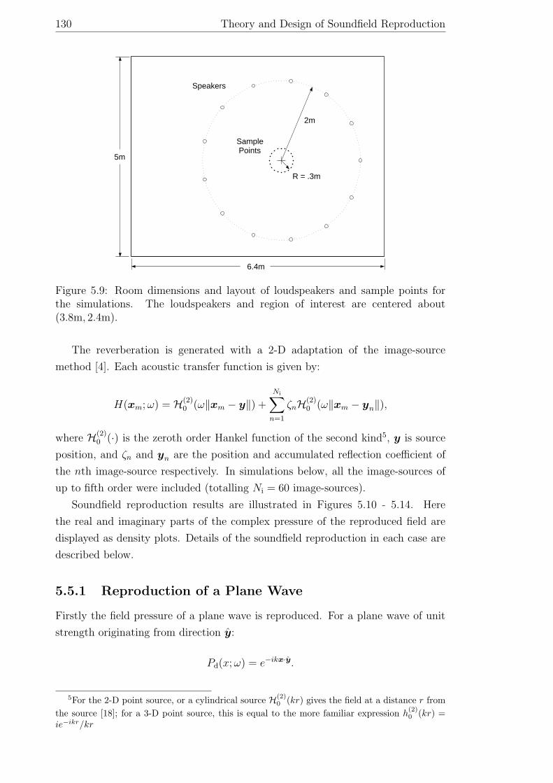
For the 2-D examples, the reverberant room parameters and loudspeaker place-
ment are summarized in Figure 5.9. The room is rectangular with a wall absorp-
tion coefficient of 0.3. Unless otherwise stated, the control region has radius 0.3m.
Though the soundfield reproduction design technique is applicable for any config-
uration and type of loudspeaker, we perform the soundfield reproduction by posi-
tioning omnidirectional loudspeakers in circular array concentric with the region
of interest. This setup yields an average DRR from each loudspeaker of −4.4dB at
the boundary of B2.
The loudspeaker requirements of this scenario are governed by the control re-
gion parameter N = dkRe = 6, prompting the use of 2N + 1 = 13 loudspeakers.
Following the conservative design procedure of Section 5.3.1 with ε = −20dB, the
maximum error scaling is κ(ω) = 25dB, and from Figure 5.4 the d∆Ne correspond-
ing to κ′(ω) = ε/κ(ω) is 14. We hence sample the pressure at M = N +d∆Ne = 20
points to measure the room response coefficients αn(`, ω).
130 Theory and Design of Soundfield Reproduction
2m
R = .3m
Sample Points
Speakers
6.4m
5m
Figure 5.9: Room dimensions and layout of loudspeakers and sample points forthe simulations. The loudspeakers and region of interest are centered about(3.8m, 2.4m).
The reverberation is generated with a 2-D adaptation of the image-source
method [4]. Each acoustic transfer function is given by:
H(xm; ω) = H(2)0 (ω‖xm − y‖) +
Ni∑n=1
ζnH(2)0 (ω‖xm − yn‖),
where H(2)0 (·) is the zeroth order Hankel function of the second kind5, y is source
position, and ζn and yn are the position and accumulated reflection coefficient of
the nth image-source respectively. In simulations below, all the image-sources of
up to fifth order were included (totalling Ni = 60 image-sources).
Soundfield reproduction results are illustrated in Figures 5.10 - 5.14. Here
the real and imaginary parts of the complex pressure of the reproduced field are
displayed as density plots. Details of the soundfield reproduction in each case are
described below.
5.5.1 Reproduction of a Plane Wave
Firstly the field pressure of a plane wave is reproduced. For a plane wave of unit
strength originating from direction y:
Pd(x; ω) = e−ikx·y.
5For the 2-D point source, or a cylindrical source H(2)0 (kr) gives the field at a distance r from
the source [18]; for a 3-D point source, this is equal to the more familiar expression h(2)0 (kr) =
ie−ikr/kr
5.5 Simulation Examples 131
Through the Jacobi-Anger expression (2.49) one sees the modal coefficients are
given by
β(d)n (ω) = (−i)ne−inφy ,
where φy is the polar angle of y. Loudspeaker filter weights are chosen using the
least squares approach of Section 5.2.4.
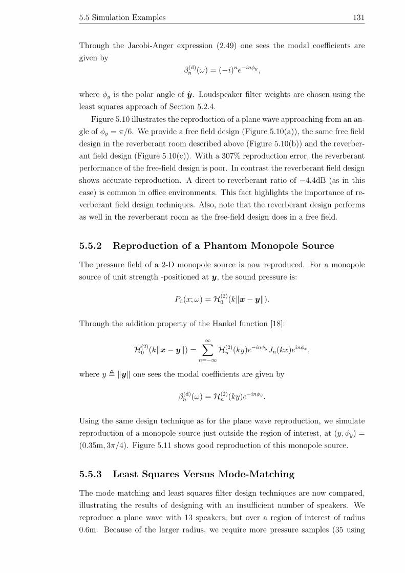
Figure 5.10 illustrates the reproduction of a plane wave approaching from an an-
gle of φy = π/6. We provide a free field design (Figure 5.10(a)), the same free field
design in the reverberant room described above (Figure 5.10(b)) and the reverber-
ant field design (Figure 5.10(c)). With a 307% reproduction error, the reverberant
performance of the free-field design is poor. In contrast the reverberant field design
shows accurate reproduction. A direct-to-reverberant ratio of −4.4dB (as in this
case) is common in office environments. This fact highlights the importance of re-
verberant field design techniques. Also, note that the reverberant design performs
as well in the reverberant room as the free-field design does in a free field.
5.5.2 Reproduction of a Phantom Monopole Source
The pressure field of a 2-D monopole source is now reproduced. For a monopole
source of unit strength -positioned at y, the sound pressure is:
Pd(x; ω) = H(2)0 (k‖x− y‖).
Through the addition property of the Hankel function [18]:
H(2)0 (k‖x− y‖) =
∞∑n=−∞
H(2)n (ky)e−inφyJn(kx)einφx ,
where y , ‖y‖ one sees the modal coefficients are given by
β(d)n (ω) = H(2)
n (ky)e−inφy .
Using the same design technique as for the plane wave reproduction, we simulate
reproduction of a monopole source just outside the region of interest, at (y, φy) =
(0.35m, 3π/4). Figure 5.11 shows good reproduction of this monopole source.
5.5.3 Least Squares Versus Mode-Matching
The mode matching and least squares filter design techniques are now compared,
illustrating the results of designing with an insufficient number of speakers. We
reproduce a plane wave with 13 speakers, but over a region of interest of radius
0.6m. Because of the larger radius, we require more pressure samples (35 using
132 Theory and Design of Soundfield Reproduction
−0.6 −0.4 −0.2 0 0.2 0.4−0.6
−0.4
−0.2
0
0.2
0.4
0.6
x (m)
y (m
)
Real
−0.6 −0.4 −0.2 0 0.2 0.4−0.6
−0.4
−0.2
0
0.2
0.4
0.6
x (m)
y (m
)
Imaginary
(a)
−0.6 −0.4 −0.2 0 0.2 0.4−0.6
−0.4
−0.2
0
0.2
0.4
0.6
x (m)
y (m
)
Real
−0.6 −0.4 −0.2 0 0.2 0.4−0.6
−0.4
−0.2
0
0.2
0.4
0.6
x (m)
y (m
)
Imaginary
(b)
−0.6 −0.3 0 0.3 0.6−0.6
−0.3
0
0.3
0.6
x (m)
y (m
)
Real
−0.6 −0.3 0 0.3 0.6−0.6
−0.3
0
0.3
0.6
x (m)
y (m
)
Imaginary
(c)
Figure 5.10: Reproduction of a plane wave with 13 speakers and 20 pressure sam-ples in a 0.3m radius circle, for (a) a free field, (b) the same free field design inthe reverberant room, and (c) a reverberant field design in the reverberant room.Reproduction errors as defined in (5.3) are 0.87%, 307% and 0.85% respectively.
conservative procedures).
For the least squares solution, speaker weights are determined from straight
forward application of (5.15). For the modal solution, one can only reproduce 13
of the 25 active modes. We choose to reproduce the lowest order modes.
The resulting sound fields are shown in Figure 5.12. While the least squares
solution reproduces the soundfield with uniform reproduction accuracy over the
whole region of interest (Figure 5.12(a)), mode-matching reproduces accurately
within a disc of radius of 0.3m as before but not outside this disc (Figure 5.12(b)).

5.5 Simulation Examples 133
−0.6 −0.3 0 0.3 0.6−0.6
−0.3
0
0.3
0.6
x (m)
y (m
)
Real
−0.6 −0.3 0 0.3 0.6−0.6
−0.3
0
0.3
0.6
x (m)
y (m
)
Imaginary
Figure 5.11: Reproduction of monopole in a 0.3m radius circle of the reverberantroom with 13 speakers and 20 pressure samples. Reproduction error as defined in(5.3) is 2.12%. The position of the monopole is marked with a ’+’.
Mode-matching fails outside this disc because the 12 highest order modes, which
become active there, are not reproduced. In general, at larger radii the higher
order modes become active but the mode matching approach, unlike least squares,
makes no attempt to reproduce them.
3 3.5 4 4.5 5
1.5
2
2.5
3
3.5
x (m)
y (m
)
Real
3 3.5 4 4.5 5
1.5
2
2.5
3
3.5
x (m)
y (m
)
Imaginary
(a)
3 3.5 4 4.5 5
1.5
2
2.5
3
3.5
x (m)
y (m
)
Real
3 3.5 4 4.5 5
1.5
2
2.5
3
3.5
x (m)
y (m
)
Imaginary
(b)
Figure 5.12: Reproduction of plane wave in a 0.6m radius circle of the reverberantroom with 13 speakers and 35 pressure samples using (a) the least squares solutionand (b) the modal solution. Reproduction errors as defined in (5.3) are 26.0% and84.1% respectively.
134 Theory and Design of Soundfield Reproduction
100 200 300 400 500 600 700 800 900 1000−50
−45
−40
−35
−30
−25
−20
−15
−10
−5
0
Frequency (Hz)
Rep
rodu
ctio
n E
rror
(dB
)
40dB SNR
30dB SNR
20dB SNR
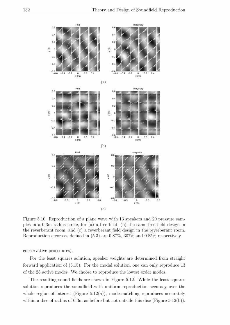
Figure 5.13: Wide-band reproduction of plane wave in a 0.3m radius circle with 13speakers and using 40 pressure samples.
5.5.4 Wide-band Reproduction with Measurement Noise
Wide-band soundfield reproduction of a plane wave is performed with noisy pres-
sure samples in the frequency range 100Hz to 1kHz, R1 = 0.3m and R2 = 0.27m.
Reproduction error is plot in Figure 5.13 for several noise SNRs averaged over
40 trial runs. This figure shows that at least 30dB SNR is required for accurate
reproduction over the whole frequency range.
The general trend in this curve is that error increases with frequency. This
trend is due to the linear increase in demand for loudspeakers and sensors with
frequency. Our design use the same number of loudspeakers and pressure samples
for all frequencies. If we desire to flatten the curve, we could use less pressure
samples and loudspeakers at lower frequencies where less modes are active.
Also observe the peaks in Figure 5.13. These peaks occur in the vicinity of the
zeros of the Bessel functions J0(kR) and J1(kR). Zeros of these Bessel functions at
460Hz and 730Hz respectively. These peaks are hence a direct result of the error
scaling mentioned in Section 5.3.3. To flatten such peaks, more pressure sampling
should be performed about these frequencies, or the sensor pairs further separated
(i.e. δR = R1 −R2 should be increased).
5.5.5 3-D Reproduction of a Plane Wave
In this 3-D example we illustrate reproduction of a plane wave in 3-space. For a 3-
D planar wave of unit strength originating from direction y, the modal coefficients

5.6 Practical Implementation 135
−0.4 −0.2 0 0.2 0.4−0.4
−0.2
0
0.2
0.4
x (m)
y (m
)
Real
−0.4 −0.2 0 0.2 0.4−0.4
−0.2
0
0.2
0.4
x (m)
y (m
)
Imaginary
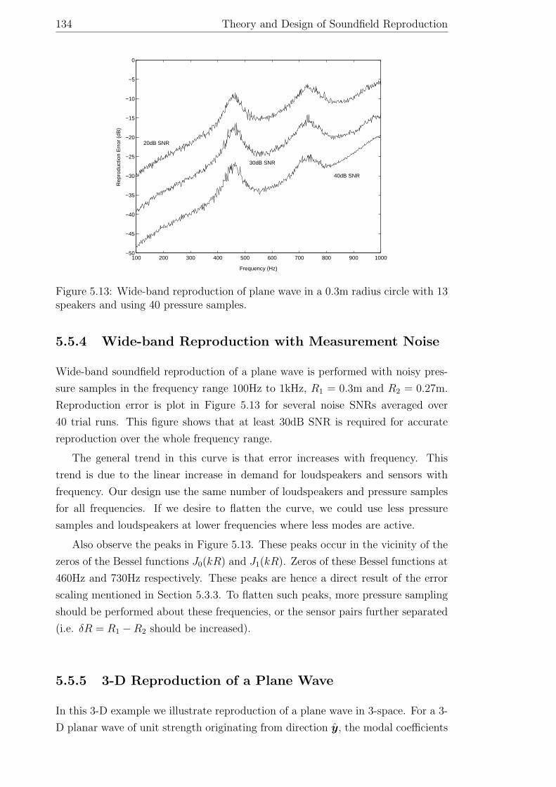
Figure 5.14: 3-D reproduction of a plane wave with 25 speakers and 49 pressuresamples in a 0.2m radius circle in a reverberant room. Reproduction error asdefined in (5.41) is 3.4%.
are given by:
βnm(ω) = 4π(−i)n[Y mn (y)]∗.
This fact can be seen by examining the Jacobi-Anger expression (2.25).
The room parameters in this simulation are similar to the 2-D case, with repro-
duction taking place in a R = 0.2m radius control region centered at (3.8m, 2.4m,
1.8m) in a 6.4×5×4m room. The reverberation is generated with the image-source
model [4] with a wall absorption coefficient of 0.3. We perform the soundfield re-
production at 2kHz by positioning (dkRe+ 1)2 = 25 omnidirectional loudspeakers
about a sphere of radius 2m as per [88] and concentric with the region of inter-
est. This setup yielded an average DRR from each loudspeaker of −4.0dB to the
boundary of B3. To measure the room response coefficients αnm(`, ω), we oversam-
pled the pressure, using M = 49 pressure samples spaces as in Figure 5.7. The
reproduction of the plane wave is illustrated in Figure 5.14.
5.6 Practical Implementation
The work presented in this chapter is still preliminary. The practical implementa-
tion of the soundfield reproduction scheme and its subjective performance remain
as open questions. Such questions shall be addressed in future research.
One important issue is sensor calibration. For measuring the modal coefficients,
the sensors have been assumed identical. If sensors are not calibrated to sufficient
accuracy, of at least 1000 : 1 for the wide-band example of Section 5.5.4, modal
coefficients will be unmeasurable. Since the gain of many real microphones changes
with temperature and humidity, accurate calibration may easily be destroyed. We
thus suggest that robustness will be a major implementation issue with this tech-
nique.
136 Theory and Design of Soundfield Reproduction
5.7 Summary and Contribution
In this chapter we have developed a novel method of performing soundfield repro-
duction in reverberant acoustical environments. Key to this method is an efficient
parametrization of the acoustic transfer function over a region of space. We provide
an itemized list of our contribution:
i. The technique of sound field reproduction through modal reconstruction has
been extended to reverberant acoustic environments. Through several simu-
lation examples, it is shown to yield a reproduction accuracy in reverberation
as good as conventional free-field designs operating in a free-field.
ii. A model-based method is provided for determining the transfer function be-
tween each loudspeaker and every point in a region. This method has arisen
from a novel interpretation of the modal space parametrization of a sound-
field.
iii. A theory for choice of fundamental design parameters has been developed -
namely the numbers of loudspeakers and sensors, geometric configuration of
sensors and loudspeaker filter weights.
Related Documents