181 Chapter 5 Simulation of dam impacts at the Searsville Lake watershed Abstract A physics-based hydrologic-response model with sediment-transport capabilities, the Integrated Hydrology Model (InHM), is used to simulate the long-term hydrologic and geomorphologic impacts of dam construction and removal for the Searsville Lake watershed in Portola Valley, California. Four dam-related scenarios (pre-dam, early dam, current, and post-dam) are considered. For each scenario an InHM boundary- value problem is constructed based on the available watershed information including topography, reservoir bathymetry, geology, soils, land use, and climate. Each scenario is simulated with InHM using the same ten-year sequence of synthetically-generated rainfall and evapotranspiration. The simulation results are presented in terms of temporal characteristics (i.e., annual water balance components, sediment discharge, and peak discharge) and spatial characteristics (i.e., maps of simulated saturation, evapotranspiration and exchange fluxes, water table elevation, and sediment concentration). An event-based sensitivity analysis indicates which model parameters exert the greatest control over the simulated watershed response and gives a measure of the parameter-related uncertainty in the model predictions. Commonalities and differences between the four scenarios are discussed. The effort described here demonstrates that physics-based modeling can provide a useful characterization of dam-related impacts on hydrologic and geomorphologic processes at the watershed scale. Heppner, Christopher S. (2007) A dam problem: characterizing the upstream hydrologic and geomorphologic impacts of dams. Ph.D. Dissertation, Department of Geological and Envrionmental Sciences, Stanford University.

Welcome message from author
This document is posted to help you gain knowledge. Please leave a comment to let me know what you think about it! Share it to your friends and learn new things together.
Transcript

181
Chapter 5
Simulation of dam impacts at the Searsville Lake watershed
Abstract A physics-based hydrologic-response model with sediment-transport capabilities,
the Integrated Hydrology Model (InHM), is used to simulate the long-term hydrologic
and geomorphologic impacts of dam construction and removal for the Searsville Lake
watershed in Portola Valley, California. Four dam-related scenarios (pre-dam, early
dam, current, and post-dam) are considered. For each scenario an InHM boundary-
value problem is constructed based on the available watershed information including
topography, reservoir bathymetry, geology, soils, land use, and climate. Each scenario
is simulated with InHM using the same ten-year sequence of synthetically-generated
rainfall and evapotranspiration. The simulation results are presented in terms of
temporal characteristics (i.e., annual water balance components, sediment discharge,
and peak discharge) and spatial characteristics (i.e., maps of simulated saturation,
evapotranspiration and exchange fluxes, water table elevation, and sediment
concentration). An event-based sensitivity analysis indicates which model parameters
exert the greatest control over the simulated watershed response and gives a measure
of the parameter-related uncertainty in the model predictions. Commonalities and
differences between the four scenarios are discussed. The effort described here
demonstrates that physics-based modeling can provide a useful characterization of
dam-related impacts on hydrologic and geomorphologic processes at the watershed
scale.
Heppner, Christopher S. (2007) A dam problem: characterizing the upstream hydrologic and geomorphologic impacts of dams. Ph.D. Dissertation, Department of Geological and Envrionmental Sciences, Stanford University.
182
5.1 Introduction
The upstream impacts of dams on hydrologic and geomorphologic watershed
processes stem from a rise in hydrologic base level. These impacts include but are not
limited to (i) inundation of previously exposed land surface, (ii) a rise in the water
table near the reservoir, (iii) decreased surface water velocities and sediment transport
capacity in the inundated channel areas, (iv) deposition of sediment in the reservoir,
and (v) evaporation from the reservoir. Dam removal, on the other hand, causes a drop
in hydrologic base level, and is expected to impact the upstream watershed in an
opposite fashion. Dam removal impacts include, for example, re-exposure of
inundated land surface, a drop in the water table near the reservoir, and net erosion of
sediment from the reservoir area. The removal of older dams, especially those whose
usefulness as a water storage location has been compromised by large upstream
sediment deposits, is becoming a more common and accepted practice (Pohl, 2003)
and can improve the ecology of the river system by reconnecting once disconnected
reaches (Gup, 1994; Ward and Stanford, 1995; Stanley et al., 2002). As dam removal
becomes more common, the issues associated with dam removal impacts are emerging
into a new cross-disciplinary field of study in the natural sciences (Grant, 2001; Doyle
et al., 2003a).
Few of the studies in this emerging field have focused on the upstream impacts of
dam removal. The downstream transport of sediment from a dam removal site has
been studied extensively (e.g., Williams, 1977; Blodgett, 1989; Simons and Simons,
1991; Stoker and Williams, 1991; Egan et al., 2000; Stillwater Sciences, 2000; Doyle
et al., 2002; Pizzuto, 2002; Stanley et al., 2002; Doyle et al., 2003b), presumably due
to concerns about sediment aggradation in the downstream channel and the possibility
of contaminated sediment exposure and mobilization. While downstream impacts
mainly concern the hydrologic and geomorphologic regime of the channel, upstream
impacts are more closely tied to the decrease in hydraulic head of the surface and
subsurface flow systems (expressed most noticeably by the decrease in surface water
depth and water table elevation) in an broader area surrounding the former reservoir
called the zone of influence. In particular, the hydrology within the zone of influence

183
can exert first-order controls over the existence of wetlands in certain topographic
settings. Therefore consideration of the upstream domain should not be overlooked
when approaching the dam removal question.
5.2 The Searsville Lake Watershed
The focus of the effort described here is the Searsville Lake watershed, in Portola
Valley, California. The 39 km2 watershed (Figure 5.1), with Searsville Dam and the
surrounding wetland at its base, provides an opportunity to examine a “real-world”
dammed system on a scale that is manageable within the physics-based modeling
approach. The fact that dam management alternatives for Searsville include dam
removal (as well as other base-level changing options such as dam lowering) also
motivates interest in this particular watershed (http://jrbp.stanford.edu/watershed.php,
accessed January 5, 2007).
5.2.1 Land Use History
The Searsville Lake watershed was inhabited for many centuries (i.e., at least
5,000 years) by indigenous people belonging to the loose-knit group of native
Americans called the Ohlone, which occupied the entire San Francisco Bay area
(Emanuels, 1994; Costo and Costo, 1995). The native people lived as hunter-gatherers
and had a light and sustainable impact on the natural surroundings. The first
Europeans to visit the area were members of the expedition up the California coast led
by the Spanish explorer Gaspar de Portola in 1769. Following the initial phase of
exploration, California was quickly settled by missionaries who established a string of
missions extending from San Diego to Solano, including the Mission Santa Clara de
Asís about 25 km east of the Searsville watershed (Hoover et al., 1990). The continued
arrival of European settlers through the middle of the 19th century brought increased
resource utilization in the area, especially in the form of logging of old-growth
redwood forests for timber. Following the dismantling of the mission system the land
was divided into ranchos, most prominently the Rancho Canada del Corte de Madera
(Hoover et al., 1990).

184
Figure 5.1. Location map for the Searsville Lake watershed showing surface water
features, land use boundaries, and locations of field measurements (see Table 5.1 for
specific measurement information). The base image is a shaded-relief DEM with a 10-
m horizontal resolution (USGS Mapping Division).
185
Today the Searsville Lake watershed is composed of a mixture of high-value
residential property, small farms and vineyards, and rugged forested slopes. Within the
watershed there are three open space preserves (i.e., Coal Creek, Windy Hill, and
Thornewood) belonging to the Mid-Peninsula Regional Open Space District, as well
as Wunderlich Park, part of the San Mateo County park system.
Construction of Searsville Dam downstream of the confluence of Corte Madera,
Sausal, Dennis Martin, and Alambique Creeks was completed in 1891 by the
Manzanita Valley Water Company. Originally intended as a water supply for Stanford
University, the lake was never used as a potable water source due to the high
concentration of suspended sediment. The lake was used for recreation for much of the
early 20th century, with grazing and scientific research occurring on Stanford-owned
lands nearby. The Jasper Ridge Biological Preserve, which includes Searsville Lake
and wetland and Jasper Ridge, was formally designated in 1973 by Stanford
University, restricting public access and dedicating the land to scientific research.
5.2.2 Watershed Properties
5.2.2.1 Geologic Setting
The Searsville watershed lies on the eastern side of the Santa Cruz Mountains, a
part of the California Coast Range. The range in elevation is from 102 m at the dam
spillway to approximately 792 m along the southeastern boundary (see Figure 5.2a).
The San Andreas Fault, shown in Figure 5.1, is a right-lateral strike-slip fault with
minor compression that traverses the watershed from southeast to northwest, defining
the linear valley along which Sausal Creek flows, and separating older Cretaceous
rocks on the north side from younger Eocene rocks on the south side. The Pilarcitos
Fault, also a right-lateral strike-slip fault, runs roughly parallel to the San Andreas
Fault. The geology of the watershed (see Figure 5.2c) has been mapped on several
occasions (e.g., Diblee, Jr., 1966; Brabb et al., 2000; Coleman, 2004). The principle
rock types are sedimentary: shales of the Lambert, San Lorenzo, and Monterey
formations; massive sandstones of the Purisima, Whiskey Hill, and Butano
formations; the weakly consolidated gravelly/ sandy conglomerate of the Santa Clara
186
Figure 5.2. Searsville Lake watershed geographic information. (a) Topographic
contours, ranging from 83 m above sea level at the catchment outlet (below the dam)
to 782 m above sea level in the southeast corner; the green contour is 190 m, the
yellow contour is 390 m, and the red contour is 630 m (adapted from USGS DEM;
Northwest Hydraulic Consultants, Inc., 2002). (b) Soil associations (after Lindsey,
1970); see Table 5.2 for texture and depth characteristics of each association. (c)
Surface geology, with units listed generally in order of increasing age (adapted from
Diblee, Jr., 1961; Brabb et al., 2000; Coleman, 2004). (d) Land cover (adapted from
the National Land Cover Database).

187

188
Formation; and unconsolidated alluvium. Small areas of intrusive basaltic rock occur
in the upper elevations of the southeast corner of the watershed. Within the Jasper
Ridge Biological Preserve and the lower foothills north of the San Andreas Fault are
outcrops of the Franciscan formation, consisting of metamorphosed marine
sedimentary and volcanic rocks, typically greenstone. Slope instability in the steep
mountainous areas has resulted in many small landslides, which are regularly re-
activated by hydrologic and seismic forces.
5.2.2.2 Hydrologic Features
The Searsville watershed contains several surface streams that flow perennially
except in the driest years (see Figure 5.1). Three major streams drain directly into the
Searsville Lake wetland from the south and west: Alambique Creek, Sausal Creek, and
Corte Madera Creek. Westridge Creek drains into Corte Madera Creek from the
eastern foothills shortly before the latter enters the wetland area. A small tributary
whose drainage area is comprised of parts of the Jasper Ridge enters Searsville Lake
from the east side. Sausal Creek and the upper reaches of Corte Madera Creek are fed
by several smaller streams which emanate from the steep forested hillslopes that make
up the entire southwestern portion of the watershed. An important tributary to Sausal
Creek is Dennis Martin Creek.
5.2.2.3 Topographic Attributes
Figure 5.3 shows certain topographic attributes of the Searsville watershed. The
map of surface slope (Figure 5.3a) clearly shows the three hydrographic areas: the
steep upland area in the west, the flat narrow valley along the San Andreas Fault Zone,
and the highly dissected foothill region on the northeast. Slopes up to 40 degrees are
present in the upland areas, where mass wasting events are common in the winter
months. Figure 5.3b shows the aspect of the land surface, with 0 and 360 degrees
corresponding to north. The main feature shown in Figure 5.3b is the distinction
between the generally northwards-facing slopes of the uplands and the generally
southwards-facing slopes of the foothills. The combination of slope and north-south

189
Figure 5.3. Topographic attributes of the Searsville watershed. (a) Slope. (b) Aspect
(0° and 360° indicate northward facing slopes, 90° indicates eastward facing slopes,
180° indicates southward facing slopes, and 270° indicates westward facing slopes).
(c) Curvature (positive values indicate convex topography and negative values
indicate concave topography). (d) Hypsometric curve (i.e., area-elevation curve).

190
Percent of area above indicated elevation
Elev
atio
nab
ove
msl
(m)
0 25 50 75 1000
100
200
300
400
500
600
700
800
(d)
360270180900
(b)
Aspect (deg)
403020151075321
(a)
Slope (deg)
321684210
-1-2-4-8-16-32
(c)
Curvature(deg)

191
aspect can have impacts on the degree of insolation and hence evapotranspiration.
Figure 5.3c shows the curvature of the land surface, highlighting hollows and ridges of
the uplands and foothill regions, and the relatively flat areas of the San Andreas Fault
Zone. It is also evident from Figure 5.3c that the foothill area has a higher drainage
density than the upland area, suggesting that the different bedrock geology of the
foothill area influences drainage network development. Figure 5.3d shows the
hypsometric curve relating land surface elevation to the watershed area below that
elevation. The curve shows the contributions of the low elevation areas between 100
and 200 m, a break in slope at the transition to the upland areas around 200 m
elevation, and the relatively minor contributions of the high elevations above 600 m.
5.3 Methods
The approach for this study was to conduct detailed physics-based simulations of
hydrologic response and sediment transport using the Integrated Hydrology Model
(InHM) (VanderKwaak, 1999), driven by the best available information. This section
describes the methods used to construct boundary-value problems for concept-
development simulations focused on the upstream effects of Searsville Dam.
5.3.1 Watershed Data Compilation
5.3.1.1 Existing Information
The existing hydrogeologic data compiled for this study include (i) spatial data
(i.e., topography, geology, soil types, land cover), (ii) historical climate information,
and (iii) historical response data (e.g., streamflow, water table depth). This
information, in concert with published sources relating surface and subsurface
attributes (e.g., soil type) to hydraulic properties (e.g., hydraulic conductivity),
provides the foundation for the InHM boundary-value problem construction, including
boundary and initial condition specifications.

192
5.3.1.2 Field Investigation
To supplement the basic geologic, geographic, and meteorological data described
in the previous section new spatially- and temporally-varying data of selected
hydrogeologic variables were obtained through field measurements. This additional
information includes semi-weekly pressure head, and soil-water content data at eight
locations over the course of one year (June 2005 to June 2006), as well as saturated
hydraulic conductivity, and stream sediment concentration at various times and
locations. The field data provide a baseline for how the watershed functions on an
annual time scale as a spatially heterogeneous system and serve as a qualitative
“reality check” for the simulated response. Figure 5.1 and Table 5.1 show,
respectively, the locations and types of field measurements made in the Searsville
watershed. The field data in their entirety are presented in Appendix C.
Figure 5.4 shows, for the period of observations, plots of (a) daily rainfall, (b)
average, minimum, and maximum pressure head, (c) average soil-water content at two
depth intervals, and (d) discharge at a gauge on San Francisquito Creek approximately
7 km downstream from Searsville Dam (drainage area is 96.9 km2). The most
prominent feature of this annual record is the contrast between the dry summer and the
wet winter, as shown by the rainfall (Figure 5.4a) and pressure head data (Figure
5.4b). The line of maximum pressure head (Figure 5.4b) corresponds to a tensiometer
installed at location #1 in the wetland (see Figure 5.1), which remained close to
saturation over the entire year. This tensiometer also was the slowest to decrease from
near-zero values (i.e., close to saturation) to lower (drier) values in the summer of
2005. The minimum pressure heads were observed at locations that were unshaded
(resulting in high evapotranspiration) and/ or topographically convex (resulting in
divergence of both surface and subsurface flow paths). The soil-water content pattern
(Figure 5.4c) generally resembles the pressure head pattern, and the topmost soil layer
(0 – 0.15 m) is wetter than the underlying layer (0.15 – 0.3 m). The wettest
measurements were again from location #1, which stayed relatively wet in May-June
2006 while the soil-water content values at all other locations were decreasing. The

193
Table 5.1. Hydrologic data collected for the Searsville watershed. _________________________________________________________________________________________________________
Location 1 Tensiometer TDR waveguide Number of hydraulic Number of suspended sediment
depth (m) length (m) conductivity measurements concentration measurements _________________________________________________________________________________________________________
1 0.20, 0.37 0.15, 0.30, 0.45 2 2 0.12, 0.31 0.15, 0.30, 0.45 2 3 0.15, 0.30 0.15, 0.30, 0.45 6 0.11, 0.25 0.15, 0.30, 0.45 7 0.13, 0.28 0.15, 0.30 9 0.13, 0.28 0.15, 0.30 10 0.14, 0.30 0.15, 0.30 11 0.15, 0.28, 0.38 0.15, 0.30 12 4 13 3 14 1 15 2 16 1 17 1 18 2 19 1 _________________________________________________________________________________________________________
1 See Figure 5.1

194
Figure 5.4. Observed data for the period from June 2005 to June 2006. (a) Daily
rainfall at the Jasper Ridge Biological Preserve (Note: rainfall data period extends
through April 27, 2006). (b) Pressure head, mean, minimum, and maximum at eight
sites. (c) Soil-water content mean at eight sites for two depth intervals. (d) Discharge
at downstream gauge (USGS gauge 11164500 San Francisquito Creek, Stanford
University, CA; Drainage area of 96.9 km2 includes Searsville watershed).

195
Rai
nfal
l(m
m)
0 100 200 3000
20
40
60
80 (a)
Pres
sure
head
(m)
0 100 200 300-10
0
MeanMinimumMaximum
(b)
Soil-
wat
erco
nten
t(%
)
0 100 200 3000
10
20
30
40
50
Mean, 0 - 0.15 mMean, 0.15 - 0.3 m
(c)
Time (days since 6/15/05)
Dis
char
ge(m
3 /s)
0 100 200 30010-3
10-2
10-1
100
101
102 (d)
196
stream discharge record (Figure 5.4d) shows many individual peaks correlated to
rainfall events, demonstrating that even at this larger watershed scale (approximately
2.5 times larger than the Searsville watershed) discharge is highly variable during the
wet season.
5.3.2 Physics-Based Simulation with InHM
To evaluate the impacts of changing boundary conditions (i.e., dam construction,
reservoir sedimentation, and dam removal) on watershed hydrologic response four
scenarios representing four different periods during the dam’s lifespan were developed
for simulation with InHM. The first scenario, “pre-dam”, represents conditions prior to
the construction of Searsville Dam. The second scenario, “early dam”, represents the
period shortly after dam construction, when the newly created reservoir was not yet
filled with deposited sediment. The third scenario, “current”, represents current (i.e.,
circa 2006) conditions, with a dammed reservoir mostly filled with sediment. The
fourth scenario, “post-dam”, represents conditions immediately following dam
removal, where the impounding structure is removed but the reservoir sediments
remain. The Searsville watershed boundary-value problem includes topographic,
hydrogeologic, and hydraulic parameterizations, as well as meteorological/
climatological forcings and boundary conditions.
5.3.2.1 Topography
Simulations with InHM necessitate a 3D mesh of triangular elements that reflects
the topography of the area. The topography for the Searsville Lake simulations was
based on three topographic datasets: (i) a digital elevation model with resolution of
10 m and 1 m in the horizontal and vertical directions, respectively (based on the
U.S.Geological Survey 7.5-minute Topographic Map Series); (ii) a survey of the 2002
topography and bathymetry of Searsville Lake and wetland with resolution of 0.6 m
(2 ft) in the vertical direction (Northwest Hydraulic Consultants Inc., 2002), used for
the current and post-dam scenarios; and (iii) a topographic map of the Searsville Lake
and wetland areas prior to dam construction (Trevor Herbert, Jasper Ridge Biological

197
Preserve, personal communication, 2006), used for the pre-dam and early dam
scenarios. The four surface meshes (i.e., one for each scenario) each contained 9,049
nodes and 17,856 triangular elements. The spacing of nodes was smallest in the lake
and wetland area and varied from 50 m along the channels to 150 m around the
watershed boundary. The triangular elements had a mean plan-view area of 2185 m2
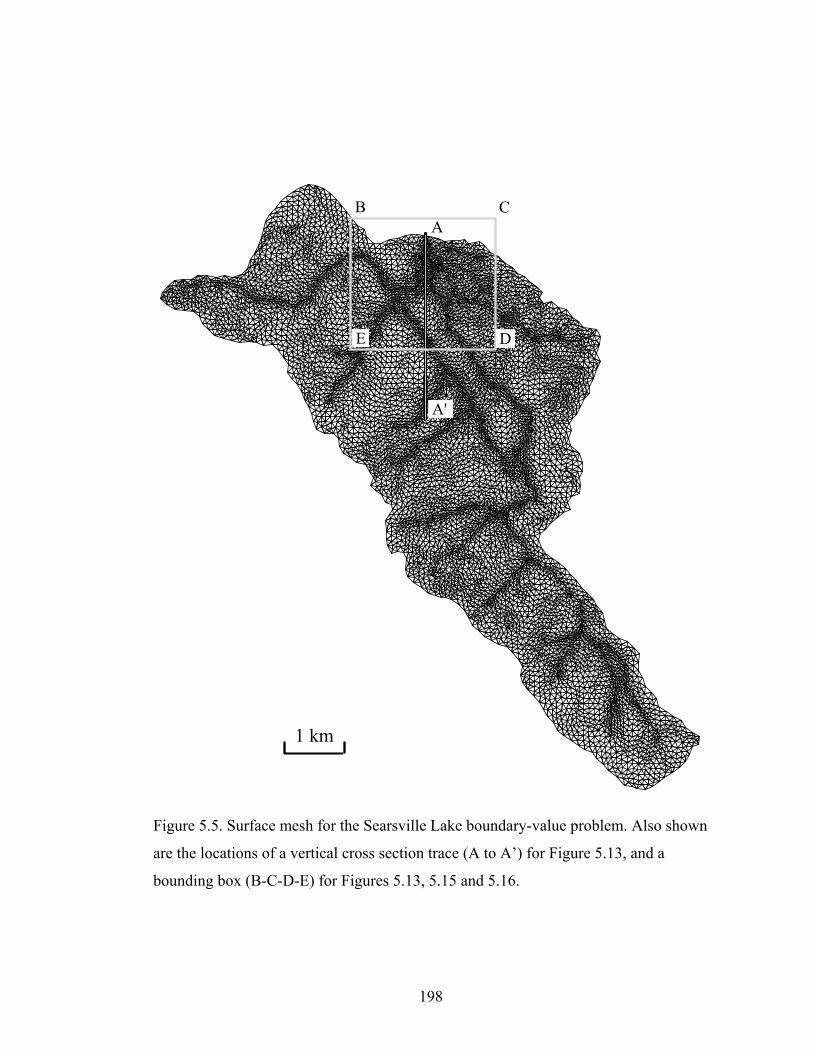
with a standard deviation of 1151 m2. Figure 5.5, depicting the surface mesh used in
this study for the current scenario, clearly shows the areas of greater detail around the
channels, Searsville Lake, and the wetland. Below the surface mesh 17 subsurface
node layers were added. The thickness of the layers varied from 0.15 m (for the top
0.6 m), to 0.3 m (for the next 0.9 m), to 2 m (for the next 10 m), and the bottom five
layers had variable exponentially-increasing thicknesses down to a base elevation of
1 m using an exponent of 1.3. The total number of nodes in the 3D mesh was 162,882.
In addition to placing node strings along the main channels of the watershed, node
strings were placed in all of the minor hollows and ridges to facilitate more realistic
flow paths in these areas.
5.3.2.2 Surface and Subsurface Parameters
To parameterize the surface and subsurface domains for simulation with InHM the
watershed was divided into multiple zones based on land cover, soil type and the
underlying bedrock type. The available land cover, soil and geologic information (see
Figure 5.2) was employed to provide sufficient detail without over-speculation of the
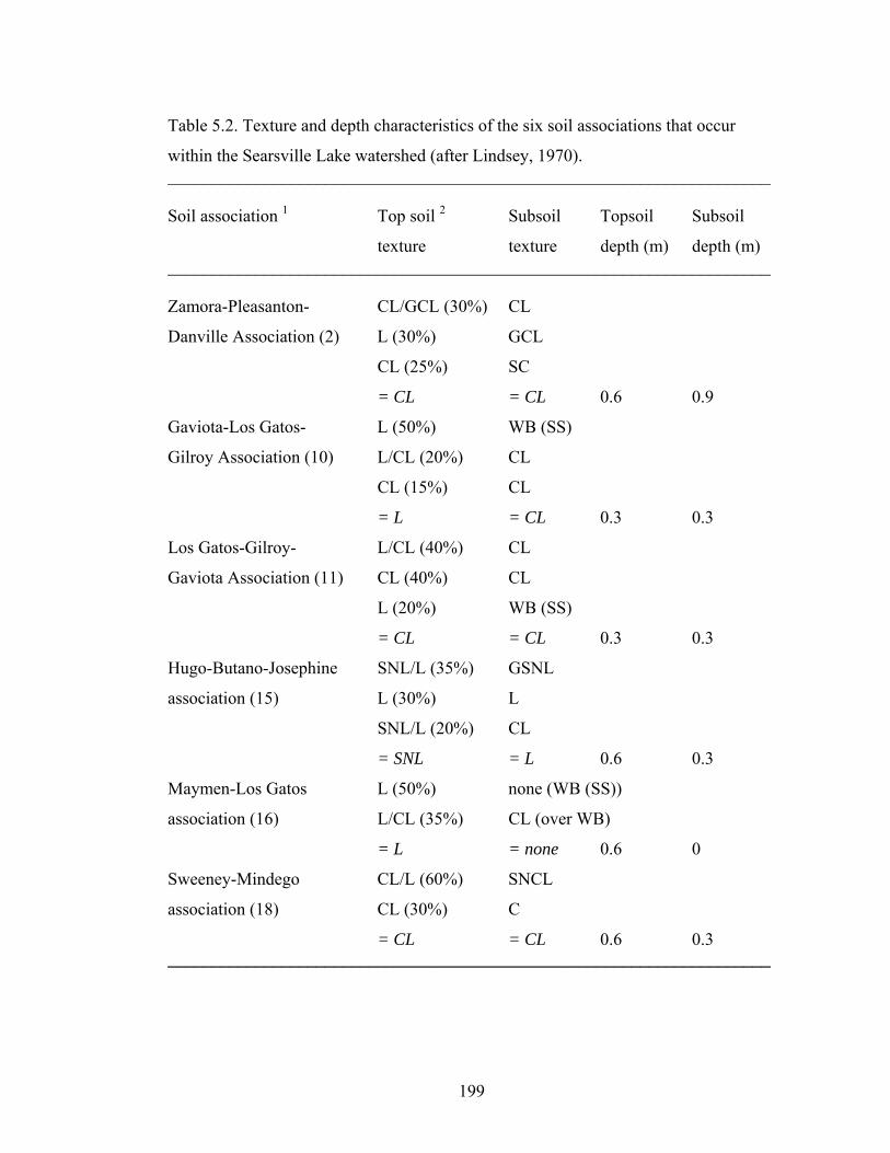
nuances in the spatial distributions. This characterization, which is summarized for
soil data in Table 5.2 and depicted graphically for soils, geology, and land use in
Figure 5.2, resulted in the division of the watershed into four land cover types (i.e.,
forest, grassland, mixed, and residential), three soil types (i.e., loam, clay loam, and
sandy loam) and six geologic units (i.e., greenstone, shale, sandstone, conglomerate,
older alluvium and recent alluvium). The three soil types were further divided into
areas underlying residential land cover (see Figure 5.2d) and all other areas, the former
assumed to have lower permeability due to greater compaction and paved area. Three
198
1 km
A
A'
B C
DE
Figure 5.5. Surface mesh for the Searsville Lake boundary-value problem. Also shown
are the locations of a vertical cross section trace (A to A’) for Figure 5.13, and a
bounding box (B-C-D-E) for Figures 5.13, 5.15 and 5.16.
199
Table 5.2. Texture and depth characteristics of the six soil associations that occur
within the Searsville Lake watershed (after Lindsey, 1970). _____________________________________________________________________ Soil association 1 Top soil 2 Subsoil Topsoil Subsoil
texture texture depth (m) depth (m) _____________________________________________________________________ Zamora-Pleasanton- CL/GCL (30%) CL
Danville Association (2) L (30%) GCL
CL (25%) SC
= CL = CL 0.6 0.9
Gaviota-Los Gatos- L (50%) WB (SS)
Gilroy Association (10) L/CL (20%) CL
CL (15%) CL
= L = CL 0.3 0.3
Los Gatos-Gilroy- L/CL (40%) CL
Gaviota Association (11) CL (40%) CL
L (20%) WB (SS)
= CL = CL 0.3 0.3
Hugo-Butano-Josephine SNL/L (35%) GSNL
association (15) L (30%) L
SNL/L (20%) CL
= SNL = L 0.6 0.3
Maymen-Los Gatos L (50%) none (WB (SS))
association (16) L/CL (35%) CL (over WB)
= L = none 0.6 0
Sweeney-Mindego CL/L (60%) SNCL
association (18) CL (30%) C
= CL = CL 0.6 0.3 _____________________________________________________________________
200
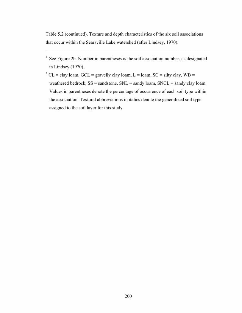
Table 5.2 (continued). Texture and depth characteristics of the six soil associations
that occur within the Searsville Lake watershed (after Lindsey, 1970). _____________________________________________________________________ 1 See Figure 2b. Number in parentheses is the soil association number, as designated
in Lindsey (1970). 2 CL = clay loam, GCL = gravelly clay loam, L = loam, SC = silty clay, WB =
weathered bedrock, SS = sandstone, SNL = sandy loam, SNCL = sandy clay loam
Values in parentheses denote the percentage of occurrence of each soil type within
the association. Textural abbreviations in italics denote the generalized soil type
assigned to the soil layer for this study

201
of the geologic units (i.e., sandstone, greenstone, and shale) were divided into
weathered (the top 10 m) and unweathered zones, with a higher permeability assigned
to the weathered condition. The conglomerate and alluvium zones were not divided
into weathered and unweathered zones because they are younger, and not yet fully
consolidated to the point where weathered zones are differentiable from the rest.
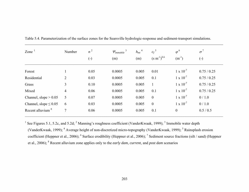
Tables 5.3 and 5.4 outline the parameterization of the subsurface and surface
zones, respectively, for the Searsville simulations. The unsaturated characteristic
relationships for the soils and bedrock (Figure 5.6) were parameterized using the van
Genuchten (1980) model for soil-water retention. For the soil zones the van Genuchten
parameters and saturated hydraulic conductivity values were based upon texture and
the catalogue of Carsel and Parrish (1988). For all other porous medium zones (i.e.,
bedrock and alluvium zones) the saturated hydraulic conductivity values and van
Genuchten parameters were estimated from published ranges (Freeze and Cherry,
1979; Wu et al., 1996).
5.3.2.3 Initial Conditions
Initial conditions, namely pressure head values at all subsurface nodes and water
depth at all surface nodes, were generated for each of the four scenarios by conducting
a one-year transient simulation starting from the following condition:
( )[ ]ZZ surft −×−== 98.0,1.0max0ψ (5.1)
where Zsurf [L] is the elevation of the land surface directly above the node and Z [L] is
the elevation of the node. This specification causes the water table to assume the form
of a subdued replica of the surface topography and the unsaturated zone to have a
minimum value (i.e., -0.1 m) for pressure head. From this specified state the one-year
simulation results in further drainage, surface water accumulation in the channels (and
reservoir for the scenarios with the dam), and a self-consistent set of hydraulic head
values in the variably-saturated subsurface. The choice of 0.98 as the surface elevation
scaling factor was driven by knowledge of the water table depth, which averages
approximately 3 to 4 m for wells at an elevation of 150 masl (Sokol, 1963).

202
Table 5.3. Parameterization of the subsurface zones for the Searsville hydrologic-
response and sediment-transport simulations. _____________________________________________________________________ Zone Ksat 1 θs 2 α 3 β 4 θr 5
(m s-1) (-) (m-1) (-) (-) _____________________________________________________________________ Sandstone 1.0 x 10⁻⁷ 0.30 4.3 1.25 0.023
Shale 1.0 x 10⁻¹¹ 0.10 4.3 1.25 0.007
Greenstone 1.0 x 10⁻⁹ 0.20 4.3 1.25 0.015
Weathered sandstone 3.0 x 10⁻⁷ 0.30 4.3 1.25 0.023
Conglomerate 1.0 x 10⁻⁵ 0.35 4.3 1.25 0.026
Weathered shale 3.0 x 10⁻¹¹ 0.10 4.3 1.25 0.007
Weathered greenstone 3.0 x 10⁻⁹ 0.20 4.3 1.25 0.015
Older alluvium 5.0 x 10⁻⁵ 0.35 14.5 2.68 0.035
Clay loam 7.2 x 10⁻⁷ 0.41 1.9 1.31 0.094
Clay loam - residential 3.6 x 10⁻⁷ 0.41 1.9 1.31 0.094
Loam 2.9 x 10⁻⁶ 0.43 3.6 1.56 0.077
Loam - residential 1.45 x 10⁻⁶ 0.43 3.6 1.56 0.077
Sandy loam 1.2 x 10⁻⁵ 0.41 7.5 1.89 0.066
Sandy loam - residential 6.0 x 10⁻⁶ 0.41 7.5 1.89 0.066
Channel deposits 2.0 x 10⁻⁴ 0.35 14.5 2.68 0.10
Recent alluvium 6 1.0 x 10⁻⁴ 0.35 14.5 2.68 0.035 _____________________________________________________________________
1 Saturated hydraulic conductivity 2 Saturated water content (porosity) 3 Parameter related to the inverse of the air-entry pressure (van Genuchten, 1980) 4 Parameter related to the pore-size distribution (van Genuchten, 1980) 5 Residual soil-water content 6 Recent alluvium zone applies only to the current and post-dam scenarios
203
Table 5.4. Parameterization of the surface zones for the Searsville hydrologic-response and sediment-transport simulations. _________________________________________________________________________________________________________ Zone 1 Number n 2 Ψimmobile 3 hmt 4 cf 5 ϕ 6 σ 7
(-) (m) (m) (s m-1)0.6 (m-1) (-) _________________________________________________________________________________________________________ Forest 1 0.05 0.0005 0.005 0.01 1 x 10⁻⁷ 0.75 / 0.25
Residential 2 0.03 0.0005 0.005 0.1 1 x 10⁻⁷ 0.75 / 0.25
Grass 3 0.10 0.0005 0.005 1 1 x 10⁻⁷ 0.75 / 0.25
Mixed 4 0.06 0.0005 0.005 0.1 1 x 10⁻⁷ 0.75 / 0.25
Channel, slope > 0.05 5 0.07 0.0005 0.005 0 1 x 10⁻⁷ 0 / 1.0
Channel, slope ≤ 0.05 6 0.03 0.0005 0.005 0 1 x 10⁻⁷ 0 / 1.0
Recent alluvium 8 7 0.06 0.0005 0.005 0.1 0 0.5 / 0.5 _________________________________________________________________________________________________________
1 See Figures 5.1, 5.2c, and 5.2d; 2 Manning’s roughness coefficient (VanderKwaak, 1999); 3 Immobile water depth
(VanderKwaak, 1999); 4 Average height of non-discretized micro-topography (VanderKwaak, 1999); 5 Rainsplash erosion
coefficient (Heppner et al., 2006); 6 Surface erodibility (Heppner et al., 2006); 7 Sediment source fractions (silt / sand) (Heppner
et al., 2006); 8 Recent alluvium zone applies only to the early dam, current, and post dam scenarios

204
Pressure head (-m)
Satu
ratio
n(-
)
Rel
ativ
epe
rmea
bilit
y(-
)10-3 10-2 10-1 100 101 102
0.1
0.2
0.3
0.4
0.5
0.6
0.70.80.9
1
10-8
10-7
10-6
10-5
10-4
10-3
10-2
10-1
100
Clay loam
Loam
Bedrock
Sandy loam
Alluvium,channels
Saturationkrel
Figure 5.6. Porous media characteristic curves for the Searsville soils, bedrock, and
alluvium.
205
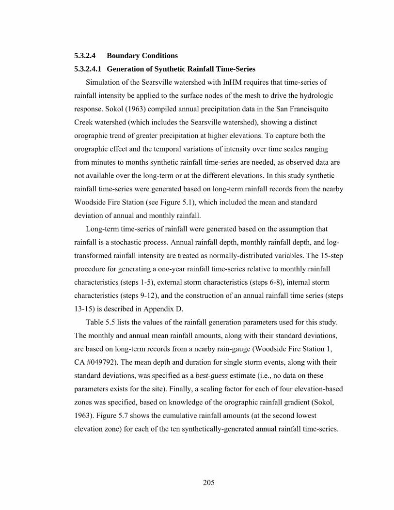
5.3.2.4 Boundary Conditions
5.3.2.4.1 Generation of Synthetic Rainfall Time-Series
Simulation of the Searsville watershed with InHM requires that time-series of
rainfall intensity be applied to the surface nodes of the mesh to drive the hydrologic
response. Sokol (1963) compiled annual precipitation data in the San Francisquito
Creek watershed (which includes the Searsville watershed), showing a distinct
orographic trend of greater precipitation at higher elevations. To capture both the
orographic effect and the temporal variations of intensity over time scales ranging
from minutes to months synthetic rainfall time-series are needed, as observed data are
not available over the long-term or at the different elevations. In this study synthetic
rainfall time-series were generated based on long-term rainfall records from the nearby
Woodside Fire Station (see Figure 5.1), which included the mean and standard
deviation of annual and monthly rainfall.
Long-term time-series of rainfall were generated based on the assumption that
rainfall is a stochastic process. Annual rainfall depth, monthly rainfall depth, and log-
transformed rainfall intensity are treated as normally-distributed variables. The 15-step
procedure for generating a one-year rainfall time-series relative to monthly rainfall
characteristics (steps 1-5), external storm characteristics (steps 6-8), internal storm
characteristics (steps 9-12), and the construction of an annual rainfall time series (steps
13-15) is described in Appendix D.
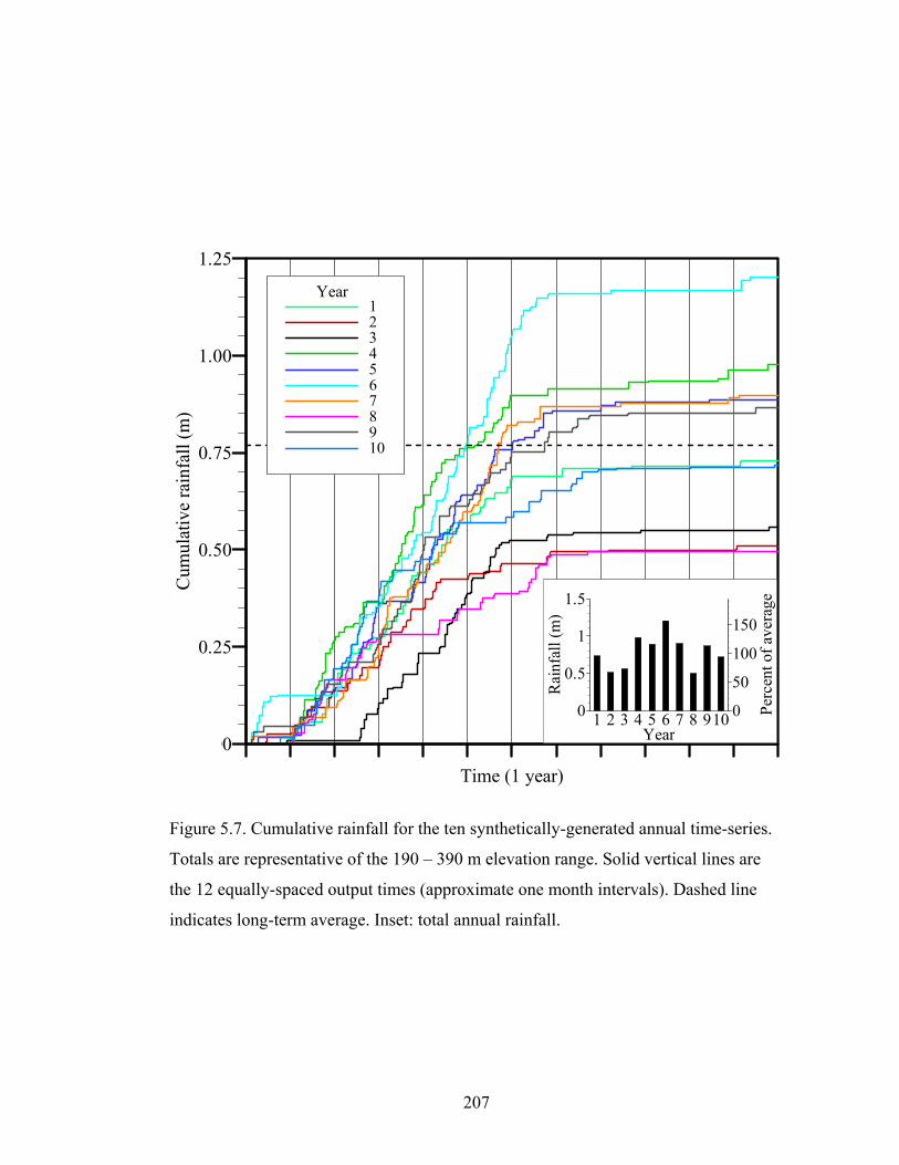
Table 5.5 lists the values of the rainfall generation parameters used for this study.
The monthly and annual mean rainfall amounts, along with their standard deviations,
are based on long-term records from a nearby rain-gauge (Woodside Fire Station 1,
CA #049792). The mean depth and duration for single storm events, along with their
standard deviations, was specified as a best-guess estimate (i.e., no data on these
parameters exists for the site). Finally, a scaling factor for each of four elevation-based
zones was specified, based on knowledge of the orographic rainfall gradient (Sokol,
1963). Figure 5.7 shows the cumulative rainfall amounts (at the second lowest
elevation zone) for each of the ten synthetically-generated annual rainfall time-series.

206
Table 5.5. Parameter values for the generation of synthetic rainfall time-series. _____________________________________________________________________
Mean Standard deviation _____________________________________________________________________ Annual rainfall depth (m) 0.768 0.295
Monthly rainfall depth (m)
January 0.153 0.107
February 0.146 0.108
March 0.117 0.081
April 0.044 0.042
May 0.018 0.024
June 0.004 0.007
July 0.001 0.003
August 0.004 0.011
September 0.007 0.010
October 0.033 0.030
November 0.101 0.088
December 0.140 0.114
Event rainfall depth (m) 0.015 0.010
Event duration (s) 43,200 21,600
Rainfall intensity (m s-1), log10 -6.5 0.5 _____________________________________________________________________ Elevation range (m) Scaling factor
80 – 190 0.86
190 – 390 1.0
390 – 630 1.11
630 – 790 1.18 _____________________________________________________________________ Storm time step (s) 900 _____________________________________________________________________
207
Time (1 year)
Cum
ulat
ive
rain
fall
(m)
0.00
0.25
0.50
0.75
1.00
1.25
12345678910
Year
Year
Rai
nfal
l(m
)
Perc
ento
fave
rage
1 2 3 4 5 6 7 8 9100
0.5
1
1.5
0
50
100
150
Figure 5.7. Cumulative rainfall for the ten synthetically-generated annual time-series.
Totals are representative of the 190 – 390 m elevation range. Solid vertical lines are
the 12 equally-spaced output times (approximate one month intervals). Dashed line
indicates long-term average. Inset: total annual rainfall.

208
5.3.2.4.2 Potential Evaporation Estimation
Potential evapotranspiration (PET) was estimated for this study using
climatological data from a weather station located in the Jasper Ridge Biological
Preserve for three areas (i.e., the grass zone; the combined forest, mixed and
residential zones; the open water area of Searsville Lake). The available data used in
this estimation included daily values of (i) maximum, minimum, and average
temperature [° C]; (ii) maximum, minimum, and average relative humidity [%]; (iii)
maximum, minimum, and average vapor pressure [kPa]; (iv) average wind velocity
[m s-1]; (v) net radiation (both short- and long-wave) [MJ m-2 d-1]; and (vi) total
photosynthetically-active radiation (PAR) [mol m-2 d-1]. The conversion of PAR to net
short-wave solar radiation [MJ m-2 d-1] assumes that PAR has a uniform distribution of
wavelengths from 400 to 700 nm, and constitutes 0.47 of the total solar radiation (the
rest arriving in infrared and ultraviolet wavelengths). All data except for the net
radiation data were from years 1997 through 2004; the net radiation data was from
2002 only. The calculations used to estimate PET are described in Appendix B.
5.4 Results
Results from the long-term simulations are presented in four sections: (i) temporal
characteristics of the simulated hydrologic response, (ii) spatial characteristics of the
simulated hydrologic response, based on snapshots extracted from the simulations,
(iii) simulated sediment characteristics, both temporal and spatial, and (iv) a
comparison of the four dam-related scenarios.
5.4.1 Temporal Characteristics of the Simulated Hydrologic Response
Table 5.6 shows the simulated surface water outflow component of the long-term
water balance. Inspection of Table 5.6 shows that year 1 and, to a lesser extent, year 2
produced high amounts of surface water outflow, especially for the pre-dam and early-
dam cases. This suggests that the watershed was still draining from the specified initial
condition, and for this reason years 1 and 2 are henceforth considered warm-up years.
The simulated results in Table 5.6 show a positive correlation between annual rainfall

209
Table 5.6. Simulated surface water outflow for the four dam-related scenarios. _____________________________________________________________________ Year Surface water outflow, mm (%) 1
Pre-dam Early dam Current Post-dam _____________________________________________________________________ 1 568 (80.8) 523 (74.4) 369 (52.6) 377 (53.7)
2 222 (45.0) 217 (44.0) 186 (37.8) 188 (38.0)
3 192 (34.8) 188 (34.0) 177 (32.0) 178 (32.3)
4 371 (39.9) 368 (39.5) 362 (38.9) 363 (39.0)
5 346 (40.4) 343 (40.0) 342 (39.8) 343 (39.9)
6 540 (46.7) 537 (46.5) 537 (46.5) 538 (46.6)
7 393 (45.5) 389 (45.1) 391 (45.3) 392 (45.5)
8 155 (32.5) 151 (31.6) 154 (32.2) 155 (32.5)
9 294 (35.1) 290 (34.7) 293 (35.0) 294 (35.1)
10 255 (36.6) 251 (36.0) 253 (36.4) 255 (36.6)
Average 334 (43.7) 326 (42.6) 306 (39.7) 308 (39.9)
Average
(years 3 – 10) 318 (38.9) 315 (38.4) 314 (38.3) 315 (38.4) _____________________________________________________________________
1 Surface water outflow is expressed both as a spatially-normalized depth of water (in
mm), and as a percentage of annual rainfall
210
and annual runoff on both absolute and percentage of rainfall bases. Years 1 and 2 are
exceptions to this pattern, showing high runoff percentages for relatively small annual
rainfall amounts, further evidence that those early years are influenced by initial
conditions. Simulated outflow ranges from approximately 150 to 540 mm yr-1, or 32 to
47 percent of annual rainfall, averaging approximately 40 percent.
Peak surface water outflow rates, shown in Table 5.7, usually occur during a given
year in response to an event with a high rank in terms of rainfall depth and peak
rainfall intensity. Peak outflow rates range from 6 to 184 m3 s-1 and vary between the
different scenarios. For all years except years 3, 4, and 7, the peak discharge occurs in
response to the same event for all four scenarios. In years 3, 4, and 7 the pre-dam
scenario has a peak discharge for a different event than the other three scenarios.
Minimum surface water outflow rates typically occur between mid-July and mid-
August, and range from approximately 0.07 to 0.14 m3 s-1.
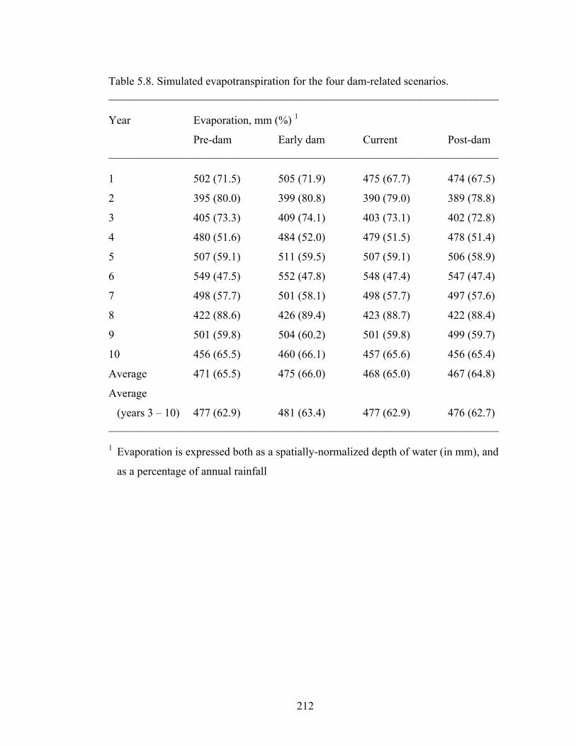
Table 5.8 shows the simulated evapotranspiration rates for the ten simulated years.
ET is positively correlated with annual rainfall, while ET as a percentage of rainfall is
negatively correlated with annual rainfall. This indicates that, although wetter near-
surface conditions occurring during rainier years contribute to enhanced ET because
more water is available, the enhancement does not keep pace with the increase in
rainfall, so the ET percentage of rainfall is smaller. The simulated ET ranges from
approximately 400 to 550 mm yr-1, and as a percentage of rainfall from 47 to 89
percent (not including years 1 and 2).
5.4.2 Spatial Characteristics of the Simulated Hydrologic Response
The distributed nature of InHM allows one to examine the spatial occurrence of
hydrological and geomorphological processes within the simulated domain.
Instantaneous snapshots of the domain are extracted from the simulations and plotted
in map view. The effects of topography, surface and porous media characteristics, and
boundary conditions can be seen in the resulting plots. The specific patterns that arise
depend, of course, on the time at which the snapshot is taken relative to previous

211
Table 5.7. Simulated peak discharge for the four dam-related scenarios. _____________________________________________________________________ Year Peak discharge (m3 s-1)
Pre-dam Early dam Current Post-dam _____________________________________________________________________ 1 69.0 58.2 47.9 48.5
2 46.0 38.9 35.6 35.9
3 40.5 29.3 26.6 26.9
4 39.4 31.5 29.2 29.5
5 47.7 33.5 30.7 30.8
6 67.4 52.7 49.2 50.1
7 35.1 30.4 29.5 29.6
8 9.9 7.3 6.3 6.3
9 184.2 158.6 147.3 149.3
10 48.2 39.5 35.7 35.8 _____________________________________________________________________
212
Table 5.8. Simulated evapotranspiration for the four dam-related scenarios. _____________________________________________________________________ Year Evaporation, mm (%) 1
Pre-dam Early dam Current Post-dam _____________________________________________________________________ 1 502 (71.5) 505 (71.9) 475 (67.7) 474 (67.5)
2 395 (80.0) 399 (80.8) 390 (79.0) 389 (78.8)
3 405 (73.3) 409 (74.1) 403 (73.1) 402 (72.8)
4 480 (51.6) 484 (52.0) 479 (51.5) 478 (51.4)
5 507 (59.1) 511 (59.5) 507 (59.1) 506 (58.9)
6 549 (47.5) 552 (47.8) 548 (47.4) 547 (47.4)
7 498 (57.7) 501 (58.1) 498 (57.7) 497 (57.6)
8 422 (88.6) 426 (89.4) 423 (88.7) 422 (88.4)
9 501 (59.8) 504 (60.2) 501 (59.8) 499 (59.7)
10 456 (65.5) 460 (66.1) 457 (65.6) 456 (65.4)
Average 471 (65.5) 475 (66.0) 468 (65.0) 467 (64.8)
Average
(years 3 – 10) 477 (62.9) 481 (63.4) 477 (62.9) 476 (62.7) _____________________________________________________________________
1 Evaporation is expressed both as a spatially-normalized depth of water (in mm), and
as a percentage of annual rainfall

213
occurrences of, for example, rainfall. In the following section all snapshots are taken
from the current scenario.
Surface-subsurface exchange fluxes result from potential gradients across the
continuum interface. Figure 5.8 illustrates several patterns that are general to all of the
scenarios. Figure 5.8a shows the exchange flux rate (m s-1) at the end of year 4, when
the catchment was in a relatively dry state, and Figure 5.8b shows the exchange flux
rate at the end of the second month of year 4, when the catchment was in a wet state.
In Figure 5.8 positive exchange flux values indicate exfiltration and negative values
indicate infiltration. The most general pattern apparent in Figure 5.8 is that exchange
fluxes tend to be strongest and in the direction of exfiltration in the channel areas and
in non-channelized concavities, and in the direction of infiltration everywhere else. An
exception to this general pattern occurs in the reservoir area, where infiltration occurs
due to the large hydrostatic pressure of the impounded water. A second pattern that is
common in the simulated snapshots is the occurrence of alternating infiltration and
exfiltration along many stretches of channel, a phenomenon which results from slight
changes in channel gradient and can be viewed as simulated hyporheic exchange (e.g.,
Harvey and Bencala, 1993; Boulton et al., 1998; Saenger et al., 2005). A third
common pattern in the simulated snapshots is that areas of infiltration tend to occur
where the steep, confined channels of the mountainous region exit onto the valley
floor area, an effect that is especially pronounced when the channels cross into a zone
underlain by the permeable older alluvium and conglomerate zones. The magnitude of
the exchange fluxes depends on the soil type as well, with lower permeability zones
associated with smaller fluxes and vice versa.
The patterns of porous media saturation at the land surface for two snapshots are
shown in Figure 5.9. The snapshots are from the same dry and wet times as those
shown in Figure 5.8. Comparison of Figures 5.9a and 5.9b shows the difference
between dry and wet periods. In both snapshots the saturation patterns reflect the
underlying soil type (see Figure 5.2b). The finer textured soils of associations 2, 11,
and 18 typically retain more water than the coarser soils of associations 10, 15, and 16.

214
1.0x10-05
1.0x10-06
1.0x10-07
1.0x10-08
0.0x10+00
-1.0x10-08
-1.0x10-07
-1.0x10-06
-1.0x10-05
Exchange flux(m s-1)
(a)
0.0
(b)
Figure 5.8. Simulated surface-subsurface exchange flux rates. (a) Year 4, end of month 12. (b) Year 4, end of month 2.

215
1.00.90.80.70.60.50.40.30.20.10.0
Saturation (-)
(a) (b)
Figure 5.9. Simulated porous medium saturation at the surface. (a) Year 4, end of month 12. (b) Year 4, end of month 2.

216
The concave areas (both channels and non-channelized areas) are generally wetter
than the convex hillslopes (see Figure 5.3c). The influence on surface saturation of the
underlying bedrock is apparent in Figure 5.9b, where areas underlain by shale are
wetter, for the same soil type, than areas underlain by sandstone. In certain portions of
the channels the saturations are very low due to the high conductivity of the channel
zone, which causes these areas to drain rapidly when not covered with surface water.
Figure 5.10 shows simulated snapshots of ET flux rate (m s-1) for the same dry
and wet times as Figure 5.8 and 5.9. Again, the role of topographic flow convergence
is shown by the higher rates of ET flux in the channels and concavities. The snapshot
in Figure 5.10a is from a time when potential ET is greater than for the time shown
Figure 5.10b, so the rates are generally higher even though soil saturation is lower. In
Figure 5.10b the effect of the hydrologic characteristics of the underlying bedrock is
seen in the greater ET flux rates from areas underlain by shale compared to areas
underlain by sandstone, a direct result of the increased saturation discussed previously.
5.4.3 Simulated Sediment Characteristics
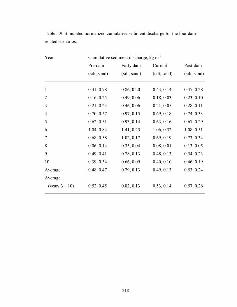
Table 5.9 shows the cumulative simulated sediment outflow for both sediment
species for each year, normalized by area (i.e., units of kg m-2 year-1). Sediment
outflow is shown to vary considerably from year to year, and has similar
characteristics as surface water outflow (i.e., it is positively correlated with the amount
of rainfall). Sediment discharge is greater in most cases for the silt-sized sediment than
for the sand-sized sediment. Total sediment outflow ranges from 0.09 to 1.88
kg m-2 year-1; outflow for the silt-sized sediment ranges from 0.06 to 1.41
kg m-2 year-1; outflow for sand-sized sediment ranges from 0.01 to 0.84 kg m-2 year-1.
Sediment concentrations at any specific location fluctuate depending on local
hydrologic conditions, sediment properties, and zone properties. Concentrations of
sand tend to be higher than silt in many channel areas due to the source fractions
assigned to this zone (i.e., 100% sand). Any increases in silt concentration in the
channel are due to influx from neighboring elements. In the reservoir area, for the
early dam and current cases, the sand concentrations tend to decrease more rapidly

217
0.0x10+00
-5.0x10⁻¹⁰
-1.0x10-09
-1.5x10-09
-2.0x10-09
-2.5x10-09
-3.0x10-09
-3.5x10-09
-4.0x10-09
-4.5x10-09
-5.0x10-09
ET flux rate(10-9 m s-1)
(a)
0.00.51.01.52.02.53.03.54.04.55.0
(b)
Figure 5.10. Simulated ET flux rate. (a) Year 4, end of month 12. (b) Year 4, end of month 2.
218
Table 5.9. Simulated normalized cumulative sediment discharge for the four dam-
related scenarios. _____________________________________________________________________ Year Cumulative sediment discharge, kg m-2
Pre-dam Early dam Current Post-dam
(silt, sand) (silt, sand) (silt, sand) (silt, sand) _____________________________________________________________________ 1 0.41, 0.78 0.86, 0.20 0.43, 0.14 0.47, 0.28
2 0.16, 0.25 0.49, 0.06 0.18, 0.03 0.23, 0.10
3 0.21, 0.23 0.46, 0.06 0.21, 0.05 0.28, 0.11
4 0.70, 0.57 0.97, 0.15 0.69, 0.18 0.74, 0.33
5 0.62, 0.51 0.93, 0.14 0.63, 0.16 0.67, 0.29
6 1.04, 0.84 1.41, 0.25 1.06, 0.32 1.08, 0.51
7 0.68, 0.58 1.02, 0.17 0.69, 0.19 0.73, 0.34
8 0.06, 0.14 0.35, 0.04 0.08, 0.01 0.13, 0.05
9 0.49, 0.41 0.78, 0.13 0.48, 0.13 0.54, 0.23
10 0.39, 0.34 0.66, 0.09 0.40, 0.10 0.46, 0.19
Average 0.48, 0.47 0.79, 0.13 0.49, 0.13 0.53, 0.24
Average
(years 3 – 10) 0.52, 0.45 0.82, 0.13 0.53, 0.14 0.57, 0.26 _____________________________________________________________________

219
after storm events due to their faster settling velocity. On hillslopes concentrations
tend to be higher for sand during rainfall events (due to greater rainsplash erosion
susceptibility, see Figure 2.2) until surface-water depths reach the mobile-water depth,
at which point overland flow and hydraulic erosion begin to occur, raising silt
concentrations rapidly as rainsplash erosion is diminished. The interactions are
complex but can be traced to the processes and/ or parameterization of InHM.
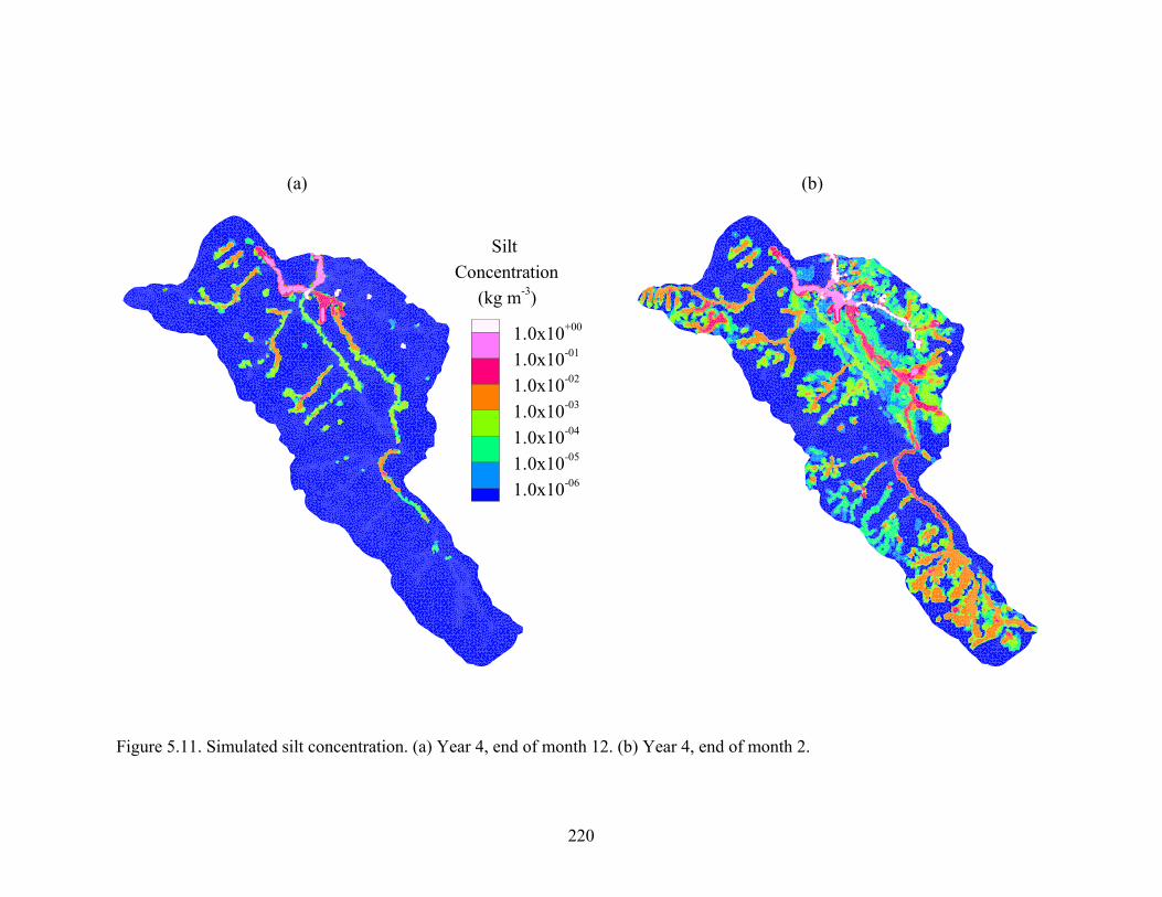
Figures 5.11 and 5.12 show pairs of snapshots of simulated sediment concentration
for silt and sand, respectively. The snapshots are from the same dry and wet times as
Figures 5.8, 5.9 and 5.10. In both pairs of snapshots the wetter time corresponds to
more widespread areas of higher concentration. Sediment concentration in the
channels is shown to increase in the downstream direction for both silt and sand. The
higher concentrations for sand relative to silt for the wetter time period shown in
Figures 5.12b and 5.11b, respectively, is due to greater susceptibility to rainsplash
erosion for sand. Contrastingly, the higher silt concentrations in the reservoir area are
caused by the slower settling velocity of silt, which leaves a greater amount in
suspension.
5.4.4 Comparison of Dam Scenarios
The simulated hydrologic-response and sediment-transport results presented in
Tables 5.6 through 5.9 show differences between the four dam-related scenarios that
are driven by differences in the scenarios’ parameterizations. These differences
include:
• Cumulative surface water outflow (Table 5.6) is typically greatest for the pre-
dam scenario, followed by the early dam, post-dam, and current scenarios. The
differences are small, especially for the later years. Relative to the current
scenario the average percent difference for surface water outflow is 2.1% for
the pre-dam scenario, 0.7% for the early dam scenario, and 0.5% for the post-
dam scenario (note, these averages exclude years 1 and 2 which are considered
warm-up years).
220
1.0x10+00
1.0x10-01
1.0x10-02
1.0x10-03
1.0x10-04
1.0x10-05
1.0x10-06
SiltConcentration
(kg m-3)
(a) (b)
Figure 5.11. Simulated silt concentration. (a) Year 4, end of month 12. (b) Year 4, end of month 2.

221
1.0x10+00
1.0x10-01
1.0x10-02
1.0x10-03
1.0x10-04
1.0x10-05
1.0x10-06
SandConcentration
(kg m-3)
(a) (b)
Figure 5.12. Simulated sand concentration. (a) Year 4, end of month 12. (b) Year 4, end of month 2.

222
• Peak surface water discharge (Table 5.7) varies consistently between the
scenarios in the following descending order: pre-dam, early dam, post-dam,
current. The differences between the pre-dam, early dam, and current scenarios
are significant. Relative to the current scenario the average percent difference
for peak discharge rate is 40.1% for the pre-dam scenario, 8.8% for the early
dam scenario, and 0.8% for the post-dam scenario.
• Cumulative ET (Table 5.8) is typically greatest for the early dam scenario,
followed by the pre-dam, current, and post-dam scenarios. Relative to the
current scenario the average percent difference for ET is 0.1% for the pre-dam
scenario, 0.8% for the early dam scenario, and -0.2% for the post-dam
scenario.
• Total normalized sediment outflow, the sum of the outflow rates for silt and
sand (Table 5.9), is generally greatest for the pre-dam scenario, followed by
the early dam, post-dam, and current scenarios. In the relatively dry years 2, 3,
and 8, the pre-dam scenario has lower sediment outflow than the early dam
scenario. For individual species, the early dam scenario consistently has the
highest discharge of silt, followed by the post-dam, current and pre-dam
scenarios (in years 4 and 9 the pre-dam scenario has marginally more silt
outflow than the current scenario). For sand the highest outflow is for the pre-
dam scenario, followed by the post-dam, current and early dam scenarios. The
proportion of total sediment outflow that is silt is highest for the early dam
scenario, followed by the current, post-dam, and pre-dam scenarios.
Beyond the cumulative and integrated measures given in Tables 5.6 through 5.9
distributed simulation allows for a spatial comparison of the four dam scenarios and
their impact on hydrologic and geomorphologic response. Figure 5.13 through 5.16
show several examples of such comparisons.
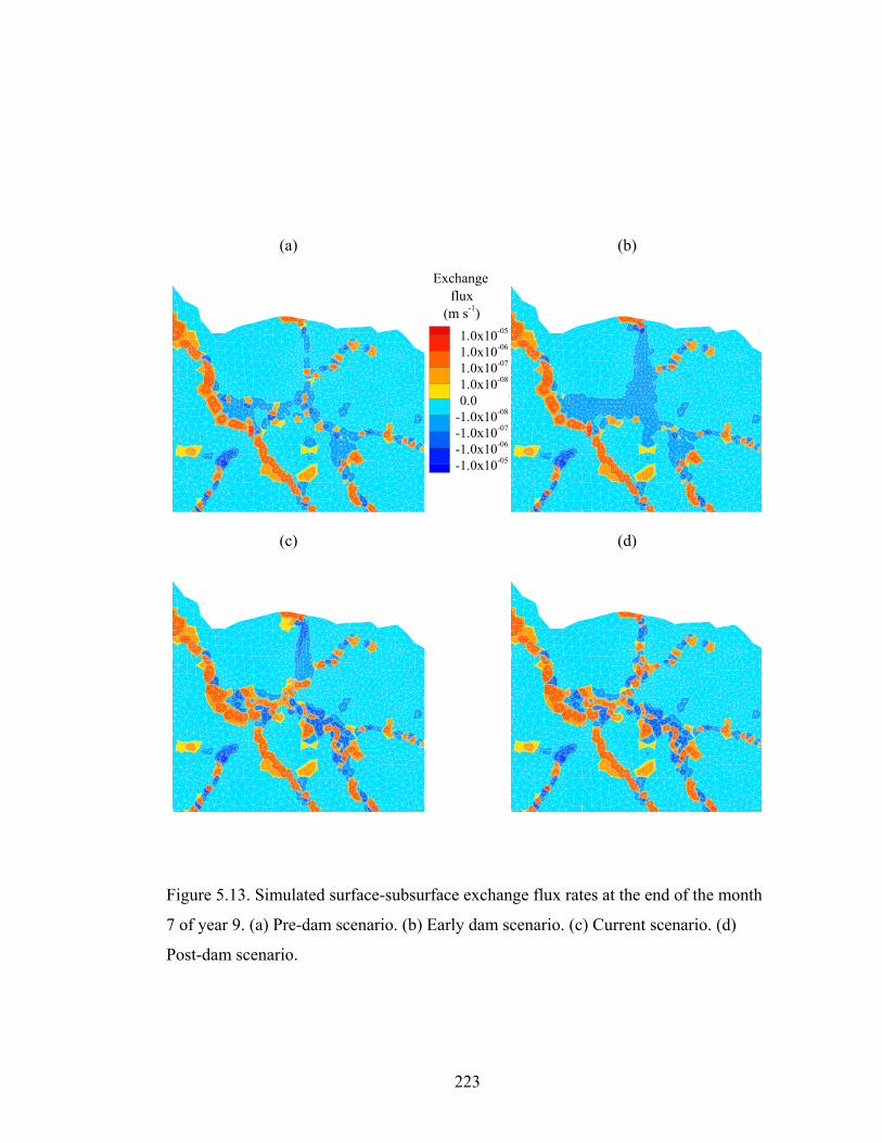
Figure 5.13 shows the simulated surface-subsurface exchange rates for the four
dam scenarios at the end of month 7 (i.e., end of April) of year 9, a time which is
neither very wet nor very dry. The area depicted in each snapshot is a close-up of the
reservoir area (box B-C-D-E in Figure 5.5). The greatest differences between the four
223
(a)
(c)
1.0x10-05
1.0x10-06
1.0x10-07
1.0x10-08
0.0x10+00
-1.0x10-08
-1.0x10-07
-1.0x10-06
-1.0x10-05
(b)
Exchangeflux
(m s-1)
(d)
Figure 5.13. Simulated surface-subsurface exchange flux rates at the end of the month
7 of year 9. (a) Pre-dam scenario. (b) Early dam scenario. (c) Current scenario. (d)
Post-dam scenario.

224
80 100 120 140 160 180 200 220 Pre-dam
Hydraulic head (m)
100 msl
(a)
Early dam
(b)
Current
(c)
Post-dam
(d)
Figure 5.14. Four vertical cross-sections through the Searsville Lake area at the end of
month 12 of year 4. (a) Pre-dam scenario. (b) Early dam scenario. (c) Current
scenario. (d) Post-dam scenario. Contours are total hydraulic head with a 1 m interval.
White lines are flow lines beginning every 250 m along the transect at an elevation of
80 m. The direction of flow is from left to right.
225
(a)
(c) (d)
2802201601101071041019895928882
Watertable
elevation(m)
(b)
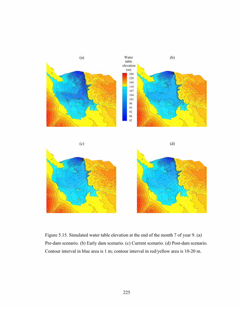
Figure 5.15. Simulated water table elevation at the end of the month 7 of year 9. (a)
Pre-dam scenario. (b) Early dam scenario. (c) Current scenario. (d) Post-dam scenario.
Contour interval in blue area is 1 m; contour interval in red/yellow area is 10-20 m.

226
(a)
(c)
1001010.10.010.0010
(b)Sandconcen-tration
(kg m-3)
(d)
Figure 5.16. Simulated sand concentration at the end of the month 7 of year 9. (a) Pre-
dam scenario. (b) Early dam scenario. (c) Current scenario. (d) Post-dam scenario.
227
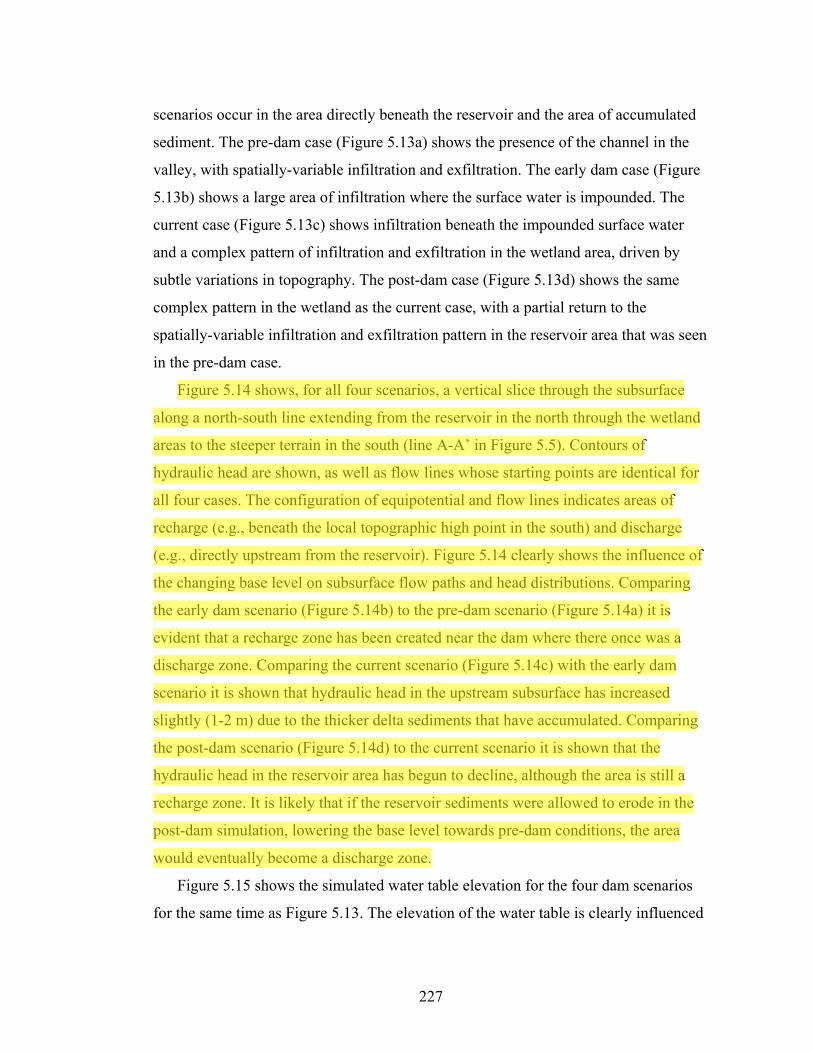
scenarios occur in the area directly beneath the reservoir and the area of accumulated
sediment. The pre-dam case (Figure 5.13a) shows the presence of the channel in the
valley, with spatially-variable infiltration and exfiltration. The early dam case (Figure
5.13b) shows a large area of infiltration where the surface water is impounded. The
current case (Figure 5.13c) shows infiltration beneath the impounded surface water
and a complex pattern of infiltration and exfiltration in the wetland area, driven by
subtle variations in topography. The post-dam case (Figure 5.13d) shows the same
complex pattern in the wetland as the current case, with a partial return to the
spatially-variable infiltration and exfiltration pattern in the reservoir area that was seen
in the pre-dam case.
Figure 5.14 shows, for all four scenarios, a vertical slice through the subsurface
along a north-south line extending from the reservoir in the north through the wetland
areas to the steeper terrain in the south (line A-A’ in Figure 5.5). Contours of
hydraulic head are shown, as well as flow lines whose starting points are identical for
all four cases. The configuration of equipotential and flow lines indicates areas of
recharge (e.g., beneath the local topographic high point in the south) and discharge
(e.g., directly upstream from the reservoir). Figure 5.14 clearly shows the influence of
the changing base level on subsurface flow paths and head distributions. Comparing
the early dam scenario (Figure 5.14b) to the pre-dam scenario (Figure 5.14a) it is
evident that a recharge zone has been created near the dam where there once was a
discharge zone. Comparing the current scenario (Figure 5.14c) with the early dam
scenario it is shown that hydraulic head in the upstream subsurface has increased
slightly (1-2 m) due to the thicker delta sediments that have accumulated. Comparing
the post-dam scenario (Figure 5.14d) to the current scenario it is shown that the
hydraulic head in the reservoir area has begun to decline, although the area is still a
recharge zone. It is likely that if the reservoir sediments were allowed to erode in the
post-dam simulation, lowering the base level towards pre-dam conditions, the area
would eventually become a discharge zone.
Figure 5.15 shows the simulated water table elevation for the four dam scenarios
for the same time as Figure 5.13. The elevation of the water table is clearly influenced
jrbp
Highlight
228
by the presence of the dam (i.e., comparing pre-dam to early dam scenarios). Water
table elevation is also influenced by the topography of the accreted sediments; it is
higher in the upper and middle lake areas (to the southwest of the main reservoir) for
the current (Figure 5.15c) and post-dam (Figure 5.15d) scenarios than for the early
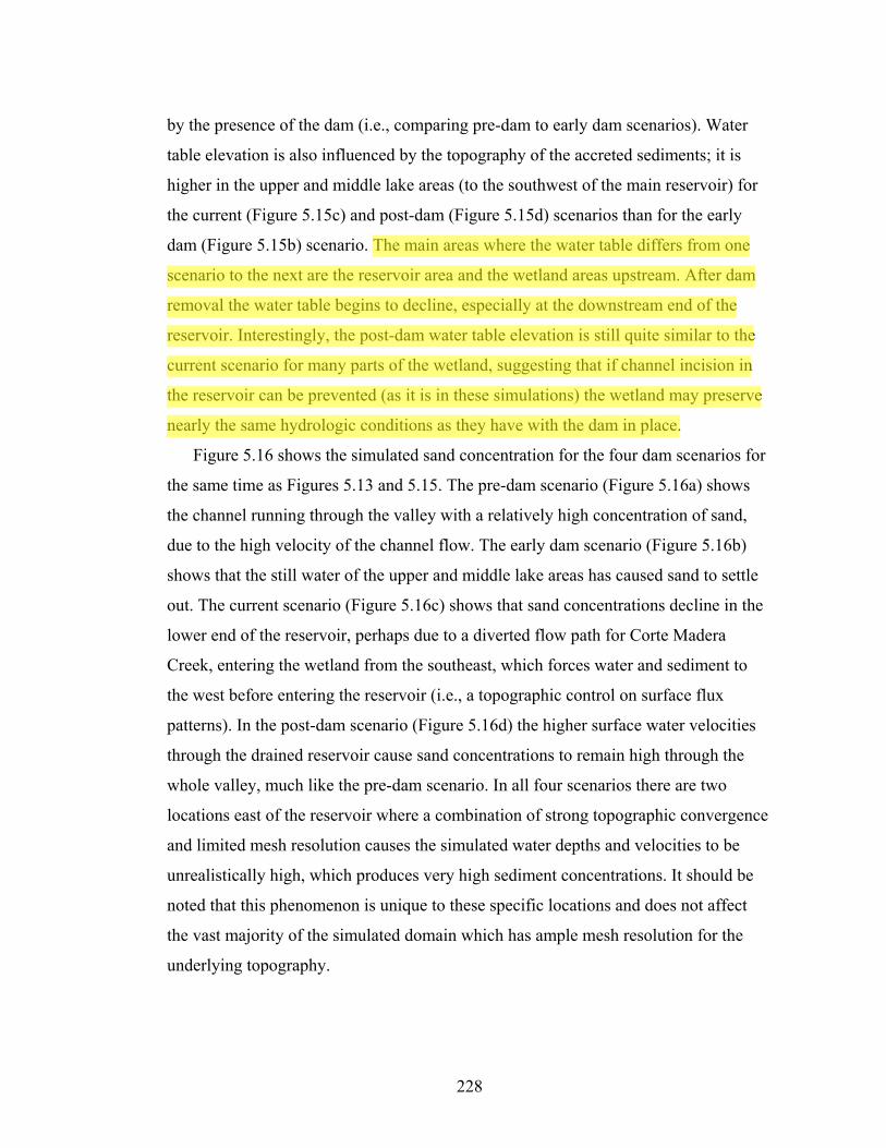
dam (Figure 5.15b) scenario. The main areas where the water table differs from one
scenario to the next are the reservoir area and the wetland areas upstream. After dam
removal the water table begins to decline, especially at the downstream end of the
reservoir. Interestingly, the post-dam water table elevation is still quite similar to the
current scenario for many parts of the wetland, suggesting that if channel incision in
the reservoir can be prevented (as it is in these simulations) the wetland may preserve
nearly the same hydrologic conditions as they have with the dam in place.
Figure 5.16 shows the simulated sand concentration for the four dam scenarios for
the same time as Figures 5.13 and 5.15. The pre-dam scenario (Figure 5.16a) shows
the channel running through the valley with a relatively high concentration of sand,
due to the high velocity of the channel flow. The early dam scenario (Figure 5.16b)
shows that the still water of the upper and middle lake areas has caused sand to settle
out. The current scenario (Figure 5.16c) shows that sand concentrations decline in the
lower end of the reservoir, perhaps due to a diverted flow path for Corte Madera
Creek, entering the wetland from the southeast, which forces water and sediment to
the west before entering the reservoir (i.e., a topographic control on surface flux
patterns). In the post-dam scenario (Figure 5.16d) the higher surface water velocities
through the drained reservoir cause sand concentrations to remain high through the
whole valley, much like the pre-dam scenario. In all four scenarios there are two
locations east of the reservoir where a combination of strong topographic convergence
and limited mesh resolution causes the simulated water depths and velocities to be
unrealistically high, which produces very high sediment concentrations. It should be
noted that this phenomenon is unique to these specific locations and does not affect
the vast majority of the simulated domain which has ample mesh resolution for the
underlying topography.
jrbp
Highlight

229
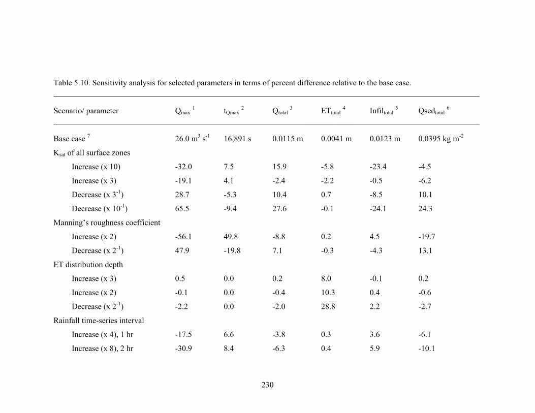
5.5 Sensitivity Analysis
Each of the four scenarios simulated in this study uses a set of parameters that is
based on the best information available. To investigate the effect of certain parameters
on the simulated hydrologic and sediment response, a sensitivity analysis is performed
for a single rainfall-runoff event. The event chosen for this analysis is a relatively
large (24 mm of rainfall) event from year four of the ten-year simulation period. The
“base case” for this analysis is the response generated by the current scenario
parameterization. The following parameters were individually adjusted: (1) the
saturated hydraulic conductivity, Ksat [LT-1], for all porous medium zones that
intersect the surface (i.e., three soil types, the same three soil types in their reduced
permeability “residential” state, the channel zone, and the recent alluvium zone); (2)
the Manning’s roughness coefficient for all surface zones; (3) the depth over which ET
is distributed; (4) the rainfall time-series interval; (5) the height of microtopography;
(6) the immobile water depth; (7) the hydraulic erosion coefficient for all surface
zones; and (8) the rainsplash erosion coefficient for all surface zones. There are 26
cases considered here, in addition to the base case. The simulations start a short
(25,200 sec) time before the beginning of the rainfall event and the initial conditions
for all cases are identical (i.e., the base case initial conditions). The results of the
sensitivity analysis, in terms of percent difference from the base case, are given in
Table 5.10.
Inspection of Table 5.10 highlights the complexity and non-linearity of near-
surface hydrologic-response processes. Runoff-generation behavior is closely tied to
the parameters that influence infiltration rate, including those that affect the land
surface’s ability to accept water from the surface (i.e., the saturated hydraulic
conductivity and the height of microtopography), those that affect the depth of
ponding and, therefore, the driving force for infiltration (i.e., the immobile water depth
and the Manning’s roughness coefficient), and those that affect the rate at which water
arrives at the surface (i.e., the rainfall time-series interval).
In general, there is an inverse correlation between the event response (i.e., total
and peak water discharge) and the simulated infiltration rate. For example, the event
230
Table 5.10. Sensitivity analysis for selected parameters in terms of percent difference relative to the base case. _________________________________________________________________________________________________________ Scenario/ parameter Qmax 1 tQmax 2 Qtotal 3 ETtotal 4 Infiltotal 5 Qsedtotal 6
_________________________________________________________________________________________________________ Base case 7 26.0 m3 s-1 16,891 s 0.0115 m 0.0041 m 0.0123 m 0.0395 kg m-2
Ksat of all surface zones
Increase (x 10) -32.0 7.5 15.9 -5.8 -23.4 -4.5
Increase (x 3) -19.1 4.1 -2.4 -2.2 -0.5 -6.2
Decrease (x 3-1) 28.7 -5.3 10.4 0.7 -8.5 10.1
Decrease (x 10-1) 65.5 -9.4 27.6 -0.1 -24.1 24.3
Manning’s roughness coefficient
Increase (x 2) -56.1 49.8 -8.8 0.2 4.5 -19.7
Decrease (x 2-1) 47.9 -19.8 7.1 -0.3 -4.3 13.1
ET distribution depth
Increase (x 3) 0.5 0.0 0.2 8.0 -0.1 0.2
Increase (x 2) -0.1 0.0 -0.4 10.3 0.4 -0.6
Decrease (x 2-1) -2.2 0.0 -2.0 28.8 2.2 -2.7
Rainfall time-series interval
Increase (x 4), 1 hr -17.5 6.6 -3.8 0.3 3.6 -6.1
Increase (x 8), 2 hr -30.9 8.4 -6.3 0.4 5.9 -10.1

231
Table 5.10 (continued). Sensitivity analysis for selected parameters in terms of percent difference relative to the base case. _________________________________________________________________________________________________________ Scenario/ parameter Qmax 1 tQmax 2 Qtotal 3 ETtotal 4 Infiltotal 5 Qsedtotal 6
_________________________________________________________________________________________________________
Rainfall time-series interval (continued)
Increase (x 20), whole event -35.2 51.8 -7.2 0.4 6.9 -11.1
Height of microtopography
Increase (x 3) 29.8 -4.1 16.9 -1.2 -16.9 16.7
Decrease (x 3-1) -2.3 0.0 -2.2 0.2 2.4 -2.2
Immobile water depth
Increase (x 3) -17.6 3.9 -10.4 0.5 8.1 -15.1
Decrease (x 3-1) 9.5 -1.5 5.4 -0.3 -4.6 6.9
Hydraulic erosion coefficient
Increase (x 10) 0 0 0 0 0 33.2
Increase (x 3) 0 0 0 0 0 9.8
Decrease (x 3-1) 0 0 0 0 0 -4.1
Decrease (x 10-1) 0 0 0 0 0 -6.1
Decrease (x 0) 0 0 0 0 0 -7.2
Rainsplash erosion coefficient
Increase (x 10) 0 0 0 0 0 -0.0

232
Table 5.10 (continued). Sensitivity analysis for selected parameters in terms of percent difference relative to the base case. _________________________________________________________________________________________________________ Scenario/ parameter Qmax 1 tQmax 2 Qtotal 3 ETtotal 4 Infiltotal 5 Qsedtotal 6
_________________________________________________________________________________________________________ Rainsplash erosion coefficient (continued)
Increase (x 3) 0 0 0 0 0 -0.1
Decrease (x 3-1) 0 0 0 0 0 -0.5
Decrease (x 10-1) 0 0 0 0 0 -0.2
Decrease (x 0) 0 0 0 0 0 -0.2 _________________________________________________________________________________________________________ 1 Peak water discharge 2 Time to peak water discharge since start of rainfall event 3 Total normalized water discharge since start of simulation 4 Total normalized evapotranspiration since start of simulation 5 Total normalized infiltration since the start of the simulation 6 Total sediment discharge since start of simulation 7 Base case values are the current scenario responses. All other entries are in terms of percent difference in response from the base
case. Base case parameter values are given in Tables 5.3 and 5.4.

233
response is increased by a decrease in the immobile water depth, which causes water
to flow rather than pond and infiltrate. Similarly, the event response is increased by an
increase in the height of microtopography, which makes the surface less saturated for
a given water depth, reducing infiltration and increasing runoff. Contrastingly, the
event response is reduced by an increase in the Manning’s roughness coefficient,
which causes water depths to be greater and slows down the surface runoff velocities,
leading to more infiltration. Increasing the rainfall time-series interval causes the
applied intensities to be less, increasing infiltration and reducing the event response, as
expected. Figure 5.17 shows the event hydrograph for all sensitivity cases that involve
a hydrologic parameter.
There are several cases in the sensitivity analysis that lead to non-intuitive event
response effects, forcing one to look deeper. The saturated hydraulic conductivity, for
example, is expected to vary inversely with event response, an assumption that holds
true for all cases except the ten-fold increase case. In the ten-fold increase case, event
response is actually augmented (and infiltration reduced), albeit with lower and time-
lagged peak discharge. The explanation for this is that the increase in conductivity
causes increased exfiltration from the most permeable channel zone that overshadows
the increased infiltration over the rest of the watershed.
Simulated ET is much less sensitive than runoff for the parameters tested. In
general, cumulative infiltration and cumulative ET are positively correlated, with
changes in infiltration causing percent changes in ET of approximately one order of
magnitude less. The largest impacts on ET result from changes to the ET distribution
depth. All three distribution depth cases (two increase cases and one decrease case)
result in increased ET. The increase in ET for decreased distribution depth is likely
caused by greater water availability due to recent rainfall in the uppermost soil layers.
The increase in ET for increased distribution depth likely results from the “tapping” by
the ET boundary condition of deeper layers that were previously untapped and
therefore had greater soil-water contents at the start of the simulation. Presumably, this
tapping effect would diminish over longer periods of simulation time until the ET rate

234
Time (sec)
Dis
char
ge(m
3s-1
)
10550000 10600000 10650000 107000000
10
20
30
40
50
Base caseHeight of microtopog. x 3-1
Height of microtopog. x 3
(b)
Time (sec)
Dis
char
ge(m
3s-1
)
10550000 10600000 10650000 107000000
10
20
30
40
50
Base caseManning' s n x 2-1
Manning' s n x 2
(c)
Time (sec)
Dis
char
ge(m
3s-1
)
10550000 10600000 10650000 107000000
10
20
30
40
50
Base caseRainfall interval x 4Rainfall interval x 8Rainfall interval x 20
(d)Time (sec)
Dis
char
ge(m
3s-1
)
10550000 10600000 10650000 107000000
10
20
30
40
50
Base caseK all surface zones x 10-1
K all surface zones x 3-1
K all surface zones x 3K all surface zones x 10
(a)
Time (sec)
Dis
char
ge(m
3s-1
)
10550000 10600000 10650000 107000000
10
20
30
40
50
Base caseET depth x 2-1
ET depth x 2ET depth x 3
(e)
Time (sec)
Dis
char
ge(m
3s-1
)
10550000 10600000 10650000 107000000
10
20
30
40
50
Base caseImmobile water depth x 3-1
Immobile water depth x 3
(f)
Figure 5.17. Hydrograph comparison of sensitivity analysis simulations versus the
base case. (a) Saturated hydraulic conductivity for all surface zones. (b) Height of
microtopography. (c) Manning’s roughness coefficient. (d) Rainfall interval length. (e)
ET distribution depth. (f) Immobile water depth.

235
became dominated by porous medium hydraulic properties, which tend to be less
permeable with increased depth (see Tables 5.2 and 5.3).
Simulated sediment discharge varies consistently with surface water outflow for
most of the sensitivity simulations involving hydrologic parameters. In most cases the
percent change in sediment discharge is roughly equal to the percent change in surface
water outflow. Sediment discharge is roughly twice as sensitive to Manning’s
roughness coefficient as surface water outflow. Sediment discharge is most sensitive
in these simulations to changes in the hydraulic erosion coefficient, although the
sensitivity is non-linear; there is a greater increase in sediment discharge for a given
increase in hydraulic erosion coefficient than there is a decrease in discharge for the
same decrease in the coefficient. The simulations are not very sensitive to the
rainsplash erosion coefficient, perhaps because the water depths are either too great to
have much rainsplash erosion (e.g., in the channels and reservoir area), or too small to
transport that sediment to the catchment outlet (e.g., on hillslopes).
Complex models like InHM require as input many physically-based (measurable)
parameters, each of which has its own degree of uncertainty. Overall, the sensitivity
simulations reported here show that the simulated response for a single event at the
Searsville watershed is quite insensitive to relatively large changes in most of the
analyzed parameters. This suggests that although the model parameterization, based in
large part on published values for similar media and/ or surfaces, contains uncertainty,
the generated response is not likely to vary significantly from the base case behavior
reported here when different values are used.
5.6 Discussion
The long-term simulations performed for this study provide, to the extent that they
are founded upon realistic descriptors of the processes and physical characteristics of
the system, insight into how the Searsville watershed system functions and how the
presence of the dam and the deposited sediments affects this functioning. In the
following paragraphs the simulation results are discussed in terms of (i) differences

236
between the four dam scenarios, (ii) impacts in the near-reservoir area, and (iii)
watershed response to varying climatic and anthropogenic forcings.
The four dam scenarios differ from each other to varying degrees depending on the
phenomenon in question. The main water balance components (Tables 5.6 and 5.8)
differ by only a few percent between the four cases for any given year. Water balance
component differences stem from varying degrees of surface-subsurface-atmosphere
exchange due to different patterns of surface-water ponding, which are ultimately
controlled by the topography of the reservoir and wetland area. Peak flow rates for
individual events do vary significantly between the four scenarios, with implications
for flood conveyance in the downstream channel. Since total surface water outflow
volume does not vary significantly, the shape, and not necessarily the integrated
volume, of event hydrographs (i.e., the timing and magnitude) is impacted the most.
Sediment discharge from the watershed does show significant differences (Table 5.9),
which can be attributed to the sensitivity of erosion and transport processes to surface
water hydraulics, differences in the zone sediment characteristics (e.g., source
fractions and erodibility coefficients), and the trapping/ retarding effects of the dam
and delta sediments.
The most important upstream impact of dam construction (or removal) is the
creation (or destruction) of a surface-water impoundment where there once was
channelized (or impounded) flow. Therefore the surface water flow regime in the
entire upstream area that lies below the dam crest elevation is profoundly affected by
dam-related activities. The simulations reported here show that upstream deposition of
sediments can result in altered surface water flow paths and depths as well. The
simulation results indicate that the zone of influence for surface water is generally
defined by the combined areas below the dam crest and where newly deposited
sediments are found (i.e., significant effects do not extend farther upstream).
Downstream from the dam the simulations indicate that channel flow (e.g., peak
discharge) is significantly altered by the dam’s construction or removal. The spatial
patterns of surface-subsurface exchange (Figure 5.13), subsurface flow nets (Figure
5.14), water table depth (Figure 5.15), and sediment concentration (Figure 5.16) all are
jrbp
Highlight
jrbp
Highlight
jrbp
Highlight
jrbp
Highlight

237
perturbed by the distinct base level and topography of each scenario, but the effects
are generally limited to areas directly under and around the reservoir and delta.
It is clear from the simulation results that climatic forcings are of first-order
importance in controlling watershed hydrologic and geomorphologic response. The
differences in response from one year to the next far outweigh the differences between
scenarios for a single year. This suggests that future watershed behavior may be
influenced much more strongly by climatic factors (e.g., changes in precipitation
amount or intensity) than by human-induced geomorphologic changes. The sensitivity
analysis reveals, however, that certain near-surface hydrogeologic and/ or land surface
characteristics affect hydrologic response in complex, non-linear ways, suggesting that
climatic or anthropogenic disturbances to these factors can significantly alter the
system behavior.
5.7 Summary
The effort reported here demonstrates an approach to characterizing the impacts of
changing base level caused by the installation and removal of a dam for the 39 km2
Searsville watershed. The approach, physics-based simulation with a comprehensive
hydrologic model with sediment-transport capabilities (InHM), is shown to be useful
in identifying and quantifying the impacts of dams. The degree of process
representation in the model, the physical basis of the parameters, and the ability to
examine both temporal and spatial patterns of hydrologic and geomorphologic
phenomena make this research approach well suited for the dam problem. This work
sets the stage for further applications of this approach to other watershed systems.
jrbp
Highlight
jrbp
Highlight
jrbp
Highlight
238
References
Blodgett, J.C., 1989, Assessment of hydraulic changes associated with the removal of
Cascade Dam, Merced River, Yosemite Valley, California, U.S. Geological Survey
Open-file Report 88-733.
Boulton, A.J., Findlay, S., Mamonier, P., Stanley, E.H., and Valett, H.M., 1998, The
Functional Significance of the Hyporheic Zone in Streams and Rivers, Annual
Reviews of Ecological Systems, v. 29, p. 59-81.
Brabb, E.E, Graymer, R.W., and Jones, D.L., 2000, Geologic map and map database
of the Palo Atlo 30’ x 60’ quadrangle, California, Pamphlet to accompany
Miscellaneous Field Studies Map MF-2332, U.S Geological Survey.
Carsel, R.F., and Parrish, R.S., 1988, Developing Joint Probability Distributions of
Soil Water Retention Characteristics, Water Resources Research v. 24, no. 5, p
755-769.
Coleman, R.G., 2004, Geologic Nature of the Jasper Ridge Biological Preserve, San
Francisco Peninsula, California, International Geology Review, v. 46, p. 629-637.
Costo, R., and Costo, J.H., 1995, Natives of the Golden State, The California Indians,
The Indian Historian Press, San Francisco, CA.
Diblee, Jr., T.W., 1966, Geologic Map and Sections of the Palo Alto 15’ Quadrangle,
California, Division of Mines and Geology, State of California, prepared in
cooperation with U.S. Geological Survey.
Doyle, M.W., Stanley, E.H., and Harbor, J.M., 2002, Geomorphic analogies for
assessing probable channel response to dam removal, Journal of the American
Water Resources Association, v. 38, no. 6, p. 1567-1579.
Doyle, M.W., Stanley, E.H., Harbor, J.M., and Grant, G.S., 2003a, Dam Removal in
the United States: Emerging Needs for Science and Policy, EOS, Transactions,
American Geophysical Union, v. 84, no. 4.
Doyle, M.W., Stanley, E.H., and Harbor, J.M., 2003b, Channel adjustments following
two dam removals in Wisconsin, Water Resources Research, v. 39, no. 1.

239
Egan, J., Pizzuto, J.E., and Mallonee, J. D., 2000, Geomorphic effects of the removal
of the Manatawny Dam, Pottstown, PA, EOS Transactions, AGU, 81(48), F515,
Fall Meeting Supplement.
Emanuels, G., 1994, California Indians, An Illustrated Guide, Kings River Press,
Lemoore, CA.
Freeze, R.A., and Cherry, J.A., 1979, Groundwater, Prentice-Hall, Englewood Cliffs,
NJ.
Grant G., 2001, Dam Removal: Panacea or Pandora for rivers?, Hydrological
Processes, v. 15, pp. 1531-1532.
Gup, T., 1994, Dammed form here to eternity: dams and biological integrity, Trout, v.
35, p. 14-20.
Harvey, J.W., and Bencala, K.E., 1993, The effect of stream bed topography on
surface-subsurface water exchange in mountain catchments, Water Resources
Research, v. 29, p. 89-98.
Heppner, C.S., Ran, Q., VanderKwaak, J.E., and Loague, K., 2006a, Adding sediment
transport to the Integrated Hydrology Model (InHM): Development and testing,
Advances in Water Resources, v. 29, p. 930-943,
doi:10.1016/j.advwatres.2005.08.003.
Hoover, M.B, Rensch, H.E., Rensch, E.G., and Abeloe, W.N., revised by D.D. Kyle,
1990, Historic Spots in California, Fourth Edition, Stanford University Press,
Stanford, CA.
Kittleson, G., Hecht, B., and Holmes, D.O., 1996, Sedimentation and Channel
Dynamics of the Searsville Lake Watershed and Jasper Ridge Biological Preserve,
San Mateo County, California, Balance Hydrologics, Inc.
Lindsey, W.C., 1970, Report and General Soil Map, San Mateo County, California,
U.S. Department of Agriculture, Soil Conservation Service.
Marschner, J., 2000, California 1850, A Snapshot in Time, Coleman Ranch Press,
Sacramento, CA.
Northwest Hydraulic Consultants, Inc., Searsville Lake Sediment Impact Study, Santa
Clara and San Mateo Counties, California, 2002.

240
Pizzuto, J., 2002, Effects of dam removal on river form and process, BioScience, v. 52,
p. 683-692.
Pohl, M.M., 2003, American Dam Removal Census: Available Data and Data Needs,
in: Dam Removal Research, Status and Prospects (Proceedings of The Heinz
Center’s Dam Removal Research Workshop, October, 2002), The H. John Heinz
III Center for Science, Economics and The Environment.
Saenger, N., Kitanidis, P.K., and Street, R.L., 2005, A numerical study of surface-
subsurface exchange processes at a riffle-pool pair in the Lahn River, Germany,
Water Resources Research,, v. 41, W12424, doi:10.1029/2004WR003875.
Simons, R.K., and Simons, D.B., 1991, Sediment problems associated with dam
removal – Muskegon River, Michigan, in R. Shane, ed., Hydraulic Engineering:
Proceedings of the National Conference on Hydraulic Engineering, ASCE, NY.
Sokol, D., 1963, The hydrogeology of the San Francisquito Creek basin, San Mateo
and Santa Clara Counties, California, Ph.D. Dissertation, Stanford University,
Stanford, CA.
Stanley, E.H., Luebke, M.A., Doyle, M.W., and Marshall, D.W., 2002, Short-term
changes in channel form and macroinvertebrate communities following low-head
dam removal, Journal of the North American Benthological Society, v. 21.
Stillwater Sciences, 2000, Technical Report, Numerical Modeling of Sediment
Transport in the Sandy River, OR Following Removal of Marmot Dam, Stillwater
Sciences, Berkeley, California for Portland General Electric, Portland, OR.
Stoker, B., and Williams, D.T., 1991, Sediment modeling of dam removal alternatives,
Elwha River, Washington, in: Shane, R.M., ed., Hydraulic engineering,
Proceedings of the national conference on hydraulic engineering, ASCE, NY, p.
674-679.
van Genuchten, M.T., 1980, A closed-form equation for predicting the hydraulic
conductivity of unsaturated soils, Soil Science Society of America Journal, v. 44, p.
892-898.
241
VanderKwaak, J.E., 1999, Numerical simulation of flow and chemical transport in
integrated surface-subsurface hydrologic systems, PhD Dissertation, University of
Waterloo, Waterloo, Ontario.
Ward, J.V., and Stanford, J.A., 1995, Ecological connectivity in alluvial river
ecosystems and its disruption by flow regulation, Regulated Rivers: Research and
Management, v. 11, p. 105-119.
Williams, D.T., Effects of dam removal: an approach to sedimentation, Technical
Paper 50, Hydrologic Engineering Center, U.S. Army Crops of Eng., Davis, CA,
1977.
Wu, Y.S., Forsyth, P.A., and Jiang, H., 1996, A consistent approach for applying
numerical boundary conditions for multiphase subsurface flow, Journal of
Contaminant Hydrology, v. 23, p. 157-184.
Related Documents