Chapter 5. Least Squares Estimation - Large-Sample Properties In Chapter 3, we assume ujx N (0; 2 ) and study the conditional distribution of b given X. In general the distribution of ujx is unknown and even if it is known, the unconditional distribution of b is hard to derive since b =(X 0 X) 1 X 0 y is a complicated function of fx i g n i=1 . Asymptotic (or large sample) methods approximate sampling distributions based on the limiting experiment that the sample size n tends to innity. A preliminary step in this approach is the demonstration that estimators converge in probability to the true parameters as the sample size gets large. The second step is to study the distributional properties of b in the neighborhood of the true value, that is, the asymptotic normality of b . The nal step is to estimate the asymptotic variance which is necessary in statistical inferences such as hypothesis testing and condence interval (CI) construction. In hypothesis testing, it is necessary to construct test statistics and derive their asymptotic distributions under the null. We will study the t-test and three asymptotically equivalent tests under both homoskedasticity and heteroskedasticity. It is also standard to develop the local power function for illustrating the power properties of the test. This chapter concentrates on asymptotic properties related to the LSE. Related materials can be found in Chapter 2 of Hayashi (2000), Chapter 4 of Cameron and Trivedi (2005), Chapter 4 of Hansen (2007), and Chapter 4 of Wooldridge (2010). 1 Asymptotics for the LSE We rst show that the LSE is CAN and then re-derive its asymptotic distribution by treating it as a MoM estimator. 1.1 Consistency It is useful to express b as b =(X 0 X) 1 X 0 y =(X 0 X) 1 X 0 (X + u)= +(X 0 X) 1 X 0 u: (1) To show b is consistent, we impose the following additional assumptions. Assumption OLS.1 0 : rank(E[xx 0 ]) = k. Assumption OLS.2 0 : y = x 0 + u with E[xu]= 0. Email: [email protected] 1

Welcome message from author
This document is posted to help you gain knowledge. Please leave a comment to let me know what you think about it! Share it to your friends and learn new things together.
Transcript

Chapter 5. Least Squares Estimation - Large-Sample Properties�
In Chapter 3, we assume ujx � N(0; �2) and study the conditional distribution of b� given
X. In general the distribution of ujx is unknown and even if it is known, the unconditionaldistribution of b� is hard to derive since b� = (X0X)�1X0y is a complicated function of fxigni=1.Asymptotic (or large sample) methods approximate sampling distributions based on the limiting
experiment that the sample size n tends to in�nity. A preliminary step in this approach is the
demonstration that estimators converge in probability to the true parameters as the sample size
gets large. The second step is to study the distributional properties of b� in the neighborhood ofthe true value, that is, the asymptotic normality of b�. The �nal step is to estimate the asymptoticvariance which is necessary in statistical inferences such as hypothesis testing and con�dence interval
(CI) construction. In hypothesis testing, it is necessary to construct test statistics and derive
their asymptotic distributions under the null. We will study the t-test and three asymptotically
equivalent tests under both homoskedasticity and heteroskedasticity. It is also standard to develop
the local power function for illustrating the power properties of the test.
This chapter concentrates on asymptotic properties related to the LSE. Related materials can
be found in Chapter 2 of Hayashi (2000), Chapter 4 of Cameron and Trivedi (2005), Chapter 4 of
Hansen (2007), and Chapter 4 of Wooldridge (2010).
1 Asymptotics for the LSE
We �rst show that the LSE is CAN and then re-derive its asymptotic distribution by treating it as
a MoM estimator.
1.1 Consistency
It is useful to express b� asb� = (X0X)�1X0y = (X0X)�1X0 (X� + u) = �+(X0X)�1X0u: (1)
To show b� is consistent, we impose the following additional assumptions.Assumption OLS.10: rank(E[xx0]) = k.
Assumption OLS.20: y = x0� + u with E[xu] = 0.
�Email: [email protected]
1

Note that Assumption OLS.10 implicitly assumes that Ehkxk2
i< 1. Assumption OLS.10 is the
large-sample counterpart of Assumption OLS.1, and Assumption OLS.20 is weaker than Assumption
OLS.2.
Theorem 1 Under Assumptions OLS.0, OLS.10, OLS.20 and OLS.3, b� p�! �.
Proof. From (1), to show b� p�! �, we need only to show that (X0X)�1X0up�! 0. Note that
(X0X)�1X0u =
1
n
nXi=1
xix0i
!�1 1
n
nXi=1
xiui
!
= g
1
n
nXi=1
xix0i;1
n
nXi=1
xiui
!p�! E[xix
0i]�1E[xiui] = 0:
Here, the convergence in probability is from (I) the WLLN which implies
1
n
nXi=1
xix0i
p�! E[xix0i] and
1
n
nXi=1
xiuip�! E[xiui]; (2)
(II) the fact that g(A;b) = A�1b is a continuous function at (E[xix0i]; E[xiui]). The last equality
is from Assumption OLS.20.
(I) To apply the WLLN, we require (i) xix0i and xiui are i.i.d., which is implied by Assumption
OLS.0 and that functions of i.i.d. data are also i.i.d.; (ii) Ehkxk2
i<1 (OLS.10) and E[kxuk] <1.
E[kxuk] <1 is implied by the Cauchy-Schwarz inequality,1
E[kxuk] � Ehkxk2
i1=2Ehjuj2i1=2
;
which is �nite by Assumption OLS.10 and OLS.3. (II) To guarantee A�1b to be a continuous
function at (E[xix0i]; E[xiui]), we must assume that E[xix0i]�1 exists which is implied by Assumption
OLS.10.2
Exercise 1 Take the model yi = x01i�1+x02i�2+ui with E[xiui] = 0. Suppose that �1 is estimated
by regressing yi on x1i only. Find the probability limit of this estimator. In general, is it consistent
for �1? If not, under what conditions is this estimator consistent for �1?
We can similarly show that the estimators b�2 and s2 are consistent for �2.Theorem 2 Under the assumptions of Theorem 1, b�2 p�! �2 and s2
p�! �2.
1Cauchy-Schwarz inequality: For any random m � n matrices X and Y, E [kX0Yk] � E�kXk2
�1=2E�kYk2
�1=2,
where the inner product is de�ned as hX;Yi = E [kX0Yk].2 If xi 2 R, E[xix0i]�1 = E[x2i ]�1 is the reciprocal of E[x2i ] which is a continuous function of E[x2i ] only if E[x2i ] 6= 0.
2

Proof. Note that
bui = yi � x0ib�= ui + x
0i� � x0ib�
= ui � x0i�b� � �� :
Thus bu2i = u2i � 2uix0i �b� � ��+ �b� � ��0 xix0i �b� � �� (3)
and
b�2 =1
n
nXi=1
bu2i=
1
n
nXi=1
u2i � 2 1
n
nXi=1
uix0i
!�b� � ��+ �b� � ��0 1n
nXi=1
xix0i
!�b� � ��p�! �2;
where the last line uses the WLLN, (2), Theorem 1 and the CMT.
Finally, since n=(n� k)! 1, it follows that
s2 =n
n� kb�2 p�! �2
by the CMT.
One implication of this theorem is that multiple estimators can be consistent for the population
parameter. While b�2 and s2 are unequal in any given application, they are close in value when nis very large.
1.2 Asymptotic Normality
To study the asymptotic normality of b�, we impose the following additional assumption.Assumption OLS.5: E[u4] <1 and E
hkxk4
i<1.
Theorem 3 Under Assumptions OLS.0, OLS.10, OLS.20, OLS.3 and OLS.5,
pn�b� � �� d�! N(0;V);
where V = Q�1Q�1 with Q = E [xix0i] and = E
�xix
0iu2i
�.
Proof. From (1),
pn�b� � �� = 1
n
nXi=1
xix0i
!�1 1pn
nXi=1
xiui
!:
3

Note �rst that
E� xix0iu2i � � E h xix0i 2i1=2E �u4i �1=2 � E hkxik4i1=2E �u4i �1=2 <1; (4)
where the �rst inequality is from the Cauchy-Schwarz inequality, the second inequality is from the
Schwarz matrix inequality,3 and the last inequality is from Assumption OLS.5. So by the CLT,
1pn
nXi=1
xiuid�! N (0;) :
Given that n�1Pni=1 xix
0i
p�! Q,
pn�b� � �� d�! Q�1N (0;) = N(0;V)
by Slutsky�s theorem.
In the homoskedastic model, V reduces to V0 = �2Q�1. We call V0 the homoskedasticcovariance matrix. Sometimes, to state the asymptotic distribution of part of b� as in the residualregression, we partition Q and as
Q =
Q11 Q12
Q21 Q21
!; =
11 12
21 22
!: (5)
Recall from the proof of the FWL theorem,
Q�1 =
Q�111:2 �Q�111:2Q12Q
�122
�Q�122:1Q21Q�111 Q�122:1
!;
where Q11:2 = Q11 � Q12Q�122 Q21 and Q22:1 = Q22 � Q21Q�111 Q12. Thus when the error is ho-moskedastic, n � AV ar
�b�1� = �2Q�111:2, and n � ACov �b�1; b�2� = ��2Q�111:2Q12Q�122 . We can alsoderive the general formulas in the heteroskedastic case, but these formulas are not easily inter-
pretable and so less useful.
Exercise 2 Of the variables (y�i ; yi;xi) only the pair (yi;xi) are observed. In this case, we say thaty�i is a latent variable. Suppose
y�i = x0i� + ui;
E[xiui] = 0;
yi = y�i + vi;
where vi is a measurement error satisfying E[xivi] = 0 and E[y�i vi] = 0. Let b� denote the OLScoe¢ cient from the regression of yi on xi.
3Schwarz matrix inequality: For any random m�n matrices X and Y, kX0Yk � kXk kYk. This is a special formof the Cauchy-Schwarz inequality, where the inner product is de�ned as hX;Yi = kX0Yk.
4

(i) Is � the coe¢ cient from the linear projection of yi on xi?
(ii) Is b� consistent for �?(iii) Find the asymptotic distribution of
pn�b� � ��.
1.3 LSE as a MoM Estimator
The LSE is a MoM estimator. The corresponding moment conditions are the orthogonal conditions
E [xu] = 0;
where u = y � x0�. So the sample analog is the normal equation
1
n
nXi=1
xi�yi � x0i�
�= 0;
the solution of which is exactly the LSE. Now, M = �E [xix0i] = �Q, and = E�xix
0iu2i
�, so
pn�b� � �� d�! N (0;V) ;
the same as in Theorem 3. Note that the asymptotic variance V takes the sandwich form. The
larger the E [xix0i], the smaller the V. Although the LSE is a MoM estimator, it is a special MoM
estimator because it can be treated as a "projection" estimator.
We provide more intuition on the asymptotic variance of b� below. Consider a simple linearregression model
yi = �xi + ui;
where E[xi] is normalized to be 0. From introductory econometrics courses,
b� =nPi=1xiyi
nPi=1x2i
=dCov(x; y)dV ar(x) ;
and under homoskedasticity,
AV ar�b�� = �2
nV ar(x):
So the larger the V ar(x), the smaller the AV ar�b��. Actually, V ar(x) = ���@E[xu]@�
���, so the intuitionin introductory courses matches the general results of the MoM estimator.
Similarly, we can derive the asymptotic distribution of the weighted least squares (WLS)estimator, a special GLS estimator with a diagonal weight matrix. Recall that
b�GLS = (X0WX)�1X0Wy;
5

which reduces to b�WLS =
nXi=1
wixix0i
!�1 nXi=1
wixiyi
!when W = diagfw1; � � � ; wng. Note that this estimator is a MoM estimator under the moment
condition
E [wixiui] = 0;
sopn�b�WLS � �
�d�! N (0;VW) ;
where VW = E [wixix0i]�1E
�w2i xix
0iu2i
�E [wixix
0i]�1.
Exercise 3 Suppose wi = ��2i , where �2i = E[u2i jxi]. Derive the asymptotic distribution of
pn�b�WLS � �
�.
2 Covariance Matrix Estimators
Since Q = E [xix0i] and = E
�xix
0iu2i
�,
bQ =1
n
nXi=1
xix0i =
1
nX0X;
and b = 1
n
nXi=1
xix0ibu2i = 1
nX0diag
�bu21; � � � ; bu2nX � 1
nX0 bDX (6)
are the MoM estimators for Q and , where fbuigni=1 are the OLS residuals. Given that V =
Q�1Q�1, it can be estimated by bV = bQ�1 bbQ�1;and AV ar(b�) is estimated by bV=n. As in (5), we can partition bQ and b accordingly and the
corresponding notations are just put a hat on. Recall from Exercise 8 of Chapter 3, V ar�b�j jX� =Pn
i=1wij�2i =SSRj . Since bV=n = (X0X)�1X0 bDX (X0X)�1 just replaces �2i in V ar �b�jX� by bu2i ,
\AV ar�b�j� =Pn
i=1wijbu2i =SSRj , j = 1; � � � ; k, where wij > 0, nPi=1wij = 1, and SSRj is the SSR in
the regression of xj on all other regressors.
Although this estimator is natural nowadays, it took some time to come into existence because
is usually expressed as E�xix
0i�2i
�whose estimation requires estimating n conditional variances. bV
appeared �rst in the statistical literature Eicker (1967) and Huber (1967), and was introduced into
econometrics by White (1980c). So this estimator is often called the "Eicker-Huber-White formula"
or something of the kind. Other popular names for this estimator include the "heteroskedasticity-
consistent (or robust) convariance matrix estimator" or the "sandwich-form convariance matrix
estimator". The following theorem provides a direct proof of the consistency of bV (although it is
6

a trivial corollary of the consistency of the MoM estimator).
Exercise 4 In the model
yi = x0i� + ui;
E[xiui] = 0; = E�xix
0iu2i
�;
�nd the MoM estimators of (�;).
Theorem 4 Under the assumptions of Theorem 3, bV p�! V.
Proof. From the WLLN, bQ is consistent. As long as we can show b is consistent, by the CMT bVis consistent. Using (3)
b =1
n
nXi=1
xix0ibu2i
=1
n
nXi=1
xix0iu2i �
2
n
nXi=1
xix0i
�b� � ��0 xiui + 1
n
nXi=1
xix0i
��b� � ��0 xi�2 .From (4), E
� xix0iu2i � <1, so by the WLLN, n�1Pni=1xix
0iu2i
p�! . We need only to prove the
remaining two terms are op(1).
Note that the second term satis�es 2nnXi=1
xix0i
�b� � ��0 xiui � 2
n
nXi=1
xix0i �b� � ��0 xiui � 2
n
nXi=1
xix0i �����b� � ��0 xi���� juij�
2
n
nXi=1
kxik3 juij! b� � � ,
where the �rst inequality is from the triangle inequality,4 and the second and third inequalities are
from the Schwarz matrix inequality. By Hölder�s inequality,5
Ehkxik3 juij
i� E
hkxik4
i3=4Ehjuij4
i1=4<1;
so by the WLLN, n�1Pni=1 kxik
3 juijp�! E
hkxik3 juij
i<1. Given that b��� = op(1), the second
4Triangle inequality: For any m� n matrices X and Y, kX+Yk � kXk+ kYk :5Hölder�s inequality: If p > 1 and q > 1 and 1
p+ 1
q= 1, then for any random m � n matrices X and Y,
E [kX0Yk] � E [kXkp]1=p E [kYkq]1=q.
7

term is op(1)Op(1) = op(1). The third term satis�es 1nnXi=1
xix0i
��b� � ��0 xi�2 � 1
n
nXi=1
xix0i ��b� � ��0 xi�2� 1
n
nXi=1
kxik4 b� � � 2 = op(1);
where the steps follow from similar arguments as in the second term.
In the homoskedastic case, we can estimateV by bV0 = b�2 bQ�1, and correspondingly,\AV ar �b�j� =n�1
Pni=1 bu2i =SSRj . In other words, the weights in the general formula take a special form,
wij = n�1. It is hard to judge which formula, homoskedasticity-only or heteroskedasticity-robust,
is larger (why?). Although either way is possible in theory, the heteroskedasticity-robust formula is
usually larger than the homoskedasticity-only one in practice; Kauermann and Carroll (2001) show
that the former is actually more variable than the latter, which is the price paid for robustness.
2.1 Alternative Covariance Matrix Estimators (*)
MacKinnon and White (1985) suggest a small-sample corrected version of bV based on the jackknife
principle which is introduced by Quenouille (1949, 1956) and Tukey (1958). Recall in Section 6 of
Chapter 3 the de�nition of b�(�i) as the least-squares estimator with the i�th observation deleted.From equation (3.13) of Efron (1982), the jackknife estimator of the variance matrix for b� is
bV� = (n� 1)nXi=1
�b�(�i) � ���b�(�i) � ��0 ; (7)
where
� =1
n
nXi=1
b�(�i):Using formula (5) in Chapter 3, we can show that
bV� =
�n� 1n
� bQ�1 b� bQ�1; (8)
where
b� = 1
n
nXi=1
(1� hi)�2xix0ibu2i � 1
n
nXi=1
(1� hi)�1xibui! 1n
nXi=1
(1� hi)�1xibui!0
and hi = x0i(X0X)�1xi. MacKinnon and White (1985) present numerical (simulation) evidence thatbV� works better than bV as an estimator of V. They also suggest that the scaling factor (n� 1)=n
in (8) can be omitted.
Exercise 5 Show that the two expressions of bV� in (7) and (8) are equal.
8
Andrews (1991) suggests a similar estimator based on cross-validation, which is de�ned by
replacing the OLS residual bui in (6) with the leave-one-out estimator bui;�i = (1 � hi)�1bui. Withthis substitution, Andrews�proposed estimator is
bV�� = bQ�1 b�� bQ�1;where b�� = 1
n
nXi=1
(1� hi)�2xix0ibu2i :It is similar to the MacKinnon-White estimator bV�, but omits the mean correction. Andrews
(1991) argues that simulation evidence indicates that bV�� is an improvement on bV�.
The jackknife represents a linear approximation of the bootstrap proposed in Efron (1979).
See Hall (1994) and Horowitz (2001) for an introduction of the bootstrap in econometrics. Other
popular books on the bootstrap and resampling methods include Efron (1982), Hall (1992), Efron
and Tibshirani (1993), Shao and Tu (1995), and Davison and Hinkley (1997).
3 Restricted Least Squares Revisited (*)
In Chapter 2, we derived the RLS estimator. We now study the asymptotic properties of the RLS
estimator. Since the RLS estimator is a special MD estimator, we concentrate on the MD estimator
under the constraints R0� = c in this section. From Exercise 26 and the discussion in Section 5.1
of Chapter 2, we can show
b�MD =b� �W�1
n R�R0W�1
n R��1 �
R0b� � c� :To derive its asymptotic distribution, we impose the following regularity conditions.
Assumption RLS.1: R0� = c where R is k � q with rank(R) = q.
Assumption RLS.2: Wnp�!W > 0:
Theorem 5 Under the Assumptions of Theorem 1, RLS.1 and RLS.2, b�MDp�! �. Under the
Assumptions of Theorem 3, RLS.1 and RLS.2,
pn�b�MD � �
�d�! N (0;VW) ;
where
VW = V �W�1R(R0W�1R)�1R0V �VR(R0W�1R)�1R0W�1
+W�1R(R0W�1R)�1R0VR(R0W�1R)�1R0W�1;
and V = Q�1Q�1:
9

From this theorem, the RLS estimator is CAN and its asymptotic variance is VQ. Unless the model
is homoskedastic, it is hard to compare VQ and V.
Exercise 6 Prove the above theorem.
The asymptotic distribution of b�MD depends on W. A natural question is which W is the
best in the sense of minimizing VW. This turns out to be V�1 as shown in the following theorem.
Since V�1 is unknown, we can replace V�1 with a consistent estimate bV�1 and the asymptotic
distribution (and e¢ ciency) are unchanged. We call the MD estimator setting Wn = bV�1 the
e¢ cient minimum distance (EMD) estimator, which takes the form
b�EMD =b� � bVR�R0 bVR��1 �R0b� � c� : (9)
Theorem 6 Under the Assumptions of Theorem 3 and RLS.1,
pn�b�EMD � �
�d�! N (0;V�) ;
where
V� = V �VR(R0VR)�1R0V:
Since
V� � V;
b�EMD has lower asymptotic variance than the unrestricted estimator. Furthermore, for any W,
V� � VW;
so b�EMD is asymptotically e¢ cient in the class of MD estimators.
Exercise 7 (i) Show that VV�1 = V�. (ii*) Show that V� � VW for any W.
Exercise 8 Consider the exclusion restriction �2 = 0 in the linear regression model yi = x01�1 +x02�2 + ui.
(i) Derive the asymptotic distribution of b�1, b�1R and b�1;EMD and show that AV ar(b�1;EMD) �AV ar(b�1) and AV ar(b�1;EMD) � AV ar(b�1R).
(ii) When the model is homoskedastic, show that AV ar(b�1;EMD) = AV ar(b�1R) � AV ar(b�1).When will the equality hold? (Hint: Q12 = 0)
(iii) When the model is heteroskedastic, provide an example where AV ar(b�1R) > AV ar(b�1).This theorem shows that the MD estimator with the smallest asymptotic variance is b�EMD.
One implication is that the RLS estimator is generally ine¢ cient. The interesting exception is the
case of conditional homoskedasticity, in which the optimal weight matrix is W = V0�1� and thus
10

the RLS estimator is an e¢ cient MD estimator. When the error is conditionally heteroskedastic,
there are asymptotic e¢ ciency gains by using minimum distance rather than least squares.
The fact that the RLS estimator is generally ine¢ cient appears counter-intuitive and requires
some re�ection to understand. Standard intuition suggests to apply the same estimation method
(least squares) to the unconstrained and constrained models, and this is the most common empirical
practice. But the above theorem shows that this is not the e¢ cient estimation method. Instead,
the EMD estimator has a smaller asymptotic variance. Why? Consider the RLS estimator with
the exclusion restrictions. In this case, the least squares estimation does not make use of the
regressor x2i. It ignores the information E [x2iui] = 0. This information is relevant when the error
is heteroskedastic and the excluded regressors are correlated with the included regressors.
Finally, note that all asymptotic variances can be consistently estimated by their sample analogs,
e.g., bV� = bV � bVR�R0 bVR��1R0 bV;where bV is a consistent estimator of V.
3.1 Orthogonality of E¢ cient Estimators
One important property of an e¢ cient estimator is the following orthogonality property popularized
by Hausman (1978).6
Theorem 7 (Orthogonality of E¢ cient Estimators) Let b� and e� be two CAN estimators of�, and e� is e¢ cient. Then the limiting distributions of pnb� and pn�e� � �� have zero covariance,where b� � b� � e�.Proof. Suppose b� and e� are not orthogonal. Since plim
�b�� = 0, consider a new estimator
� = e� + aAb�, where a is a scalar and A is an arbitrary matrix to be chosen. The new estimator
is CAN with asymptotic variance
V ar(�) = V ar(e�) + aACov(e�; b�) + aCov(e�; b�)0A0 + a2AV ar(b�)A0:Since e� is e¢ cient, the minimizer of V ar(�) with respect to a is achieved at a = 0. Taking the
�rst-order derivative with respect to a yields
AC+C0A0 + 2aAV ar(b�)A0;where C � Cov(e�; b�). Choosing A = �C0, we have
�2C0C+ 2aC0V ar(b�)C:6See also Lehmann and Casella (1998, Theorem 1.7, p85) and Rao (1973, Theorem 51.2.(i), p317) for a similar
result. Lehmann and Casella cite Barankin (1949), Stein (1950), Bahadur (1957), and Luenberger (1969) as earlyreferences.
11

Therefore, at a = 0, this derivative is equal to �2C0C � 0. Unless C = 0, we may have a better
estimator than e� by choosing a a little bit deviating from 0.
Exercise 9 (Finite-Sample Orthogonality of E¢ cient Estimators) In the homoskedastic lin-ear regression model, check Cov
� b� � b�R; b�R���X� = 0 directly. (Hint: recall that b�R = PS?X0XSb�+
(I�PS?X0XS)s:)
A direct corollary of the above theorem is as follows.
Corollary 1 Let b� and e� be two CAN estimators of �, and e� is e¢ cient. Then AV ar(b� � e�) =AV ar(b�)�AV ar(e�).3.2 Misspeci�cation
We usually have two methods to study the e¤ects of misspeci�cation of the restrictions. In Method
I, we assume the truth is R0� = c� with c� 6= c; in Method II, we assume the truth is R0�n =
c + n�1=2�. The speci�cation in Method II need some explanation. In this speci�cation, the
constraint is "close" to correct, as the di¤erence R0�n � c = n�1=2� is "small" in the sense that
it decreases with sample size n. We call such a misspeci�cation as local misspeci�cation. Thereason why the deviation is proportional to n�1=2 is because this is the only choice under which
the localizing parameter � appears in the asymptotic distribution but does not dominate it. We
will give more discussions on this choice of rate in studying the local power of tests.
First discuss Method I. From the expression of b�MD, it is not hard to see that
b�MDp�! ��MD = � �W�1R(R0W�1R)�1(c� � c):
The second term,W�1R(R0W�1R)�1(c� � c), shows that imposing an incorrect constraint leadsto inconsistency - an asymptotic bias. We call the limiting value ��MD the minimum-distance
projection coe¢ cient or the pseudo-true value implied by the restriction. There are more to say.
De�ne
��n = � �W�1n R(R
0W�1n R)
�1(c� � c):
(Note that ��n is di¤erent from ��MD.) Then
pn�b�MD � ��n
�=
pn�b� � ���W�1
n R(R0W�1
n R)�1pn
�R0b� � c�� (10)
=�I�W�1
n R(R0W�1
n R)�1R0
�pn�b� � ��
d�!�I�W�1R(R0W�1R)�1R0
�N(0;V)
= N(0;VW):
In particular,pn�b�EMD � ��n
�d�! N(0;V�):
12

This means that even when the constraint R0� = c is misspeci�ed, the conventional covariance
matrix estimator is still an appropriate measure of the sampling variance, though the distribution is
centered at the pseudo-true values (or projections) ��n rather than �. The fact that the estimators
are biased is an unavoidable consequence of misspeci�cation.
In Method II, since the true model is yi = x0i�n + ui, it is not hard to show that
pn�b� � �n� d�! N(0;V) (11)
which is the same as when � is �xed. A di¤erence arises in the constrained estimator. Since
c = R0�n � n�1=2�,R0b� � c = R0 �b� � �n�+ n�1=2�;
and
b�MD = b� �W�1n R
�R0W�1
n R��1 �
R0b� � c�= b� �W�1
n R�R0W�1
n R��1
R0�b� � �n�+ n�1=2W�1
n R�R0W�1
n R��1
�:
It follows that
pn�b�MD � �n
�d�!�I�W�1
n R(R0W�1
n R)�1R0
�pn�b� � �n�+W�1
n R�R0W�1
n R��1
�:
The �rst term is asymptotically normal by (11). The second term converges in probability to a
constant. This is because the n�1=2 local scaling is exactly balanced by thepn scaling of the
estimator. No alternative rate would have produced this result. Consequently, we �nd that the
asymptotic distribution equals
pn�b�MD � �n
�d�! N (0;VW) +W
�1R�R0W�1R
��1� = N (��;VW) ; (12)
where
�� =W�1R(R0W�1R)�1�:
The asymptotic distribution (12) is an approximation of the sampling distribution of the re-
stricted estimator under misspeci�cation. The distribution (12) contains an asymptotic bias com-
ponent ��. The approximation is not fundamentally di¤erent from (10) - they both have the same
asymptotic variances, and both re�ect the bias due to misspeci�cation. The di¤erence is that (10)
puts the bias on the left-side of the convergence arrow, while (12) has the bias on the right-side.
There is no substantive di¤erence between the two, but (12) is more convenient for some purposes,
such as the analysis of the power of tests, as we will explore in the last section of this chapter.
13

3.3 Nonlinear and Inequality Restrictions
In some cases it is desirable to impose nonlinear constraints on the parameter vector �. They can
be written as
r(�) = 0; (13)
where r: Rk ! Rq. This includes the linear constraints as a special case. An example of (13) whichcannot be written in a linear form is �1�2 = 1, which is (13) with r(�) = �1�2 � 1.
The RLS and MD estimators of � subject to (13) solve the minimization problems
b�R = arg minr(�)=0
SSR(�);
b�MD = arg minr(�)=0
Jn(�):
The solutions can be achieved by the Lagrangian method. Computationally, there is in general no
explicit expression for the solutions so they must be found numerically. Algorithms to numerically
solve such Lagrangian problems are known as constrained optimization methods, and are available
in programming languages such as Matlab.
The asymptotic distributions of b�R and b�MD are the same as in the linear constraints case
except that R is replaced by @r(�)0=@�, but the proof is more delicate.
We sometimes impose inequality constraints on �,
r(�) � 0:
The most common example is a non-negative constraint �1 � 0. The RLS and MD estimators of� can be written as
b�R = arg minr(�)�0
SSR(�);
b�MD = arg minr(�)�0
Jn(�):
Except in special cases the constrained estimators do not have simple algebraic solutions. An
important exception is when there is a single non-negativity constraint, e.g., �1 � 0 with q = 1.
In this case the constrained estimator can be found by a two-step approach. First compute the
unconstrained estimator b�. If b�1 � 0 then b�R = b�MD = b�. Second, if b�1 < 0 then impose
�1 = 0 (eliminate the regressor x1) and re-estimate. This yields the constrained least-squares
estimator. While this method works when there is a single non-negativity constraint, it does not
immediately generalize to other contexts. The computational problems with inequality constraints
are examples of quadratic programming problems. Quick and easy computer algorithms are available
in programming languages such as Matlab.
Exercise 10 (Ridge Regression) Suppose the nonlinear constraints are �0�� � B, where � >
14

0 and B > 0. Show that b�R = �X0X+ b����1X0y;where b� is the Lagrange multiplier for the constraint �0�� � B.
Inference on inequality-constrained estimators is unfortunately quite challenging. The conven-
tional asymptotic theory gives rise to the following dichotomy. If the true parameter satis�es the
strict inequality r(�) > 0, then asymptotically the estimator is not subject to the constraint and
the inequality-constrained estimator has an asymptotic distribution equal to the unconstrained one.
However if the true parameter is on the boundary, e.g., r(�) = 0, then the estimator has a truncated
structure. This is easiest to see in the one-dimensional case. If we have an estimator b� which satis�espn�b� � �� d�! Z = N(0; V ) and � = 0, then the constrained estimator b�R(= b�MD)= max
nb�; 0owill have the asymptotic distribution
pnb�R d�! max fZ; 0g, a �half-normal�distribution.
4 Functions of Parameters
Sometimes we are interested in some lower-dimensional function of the parameter vector � =
(�1; � � � ; �k)0. For example, we may be interested in a single coe¢ cient �j or a ratio �j=�l. Inthese cases we can write the parameter of interest as a function of �. Let r: Rk ! Rq denote thisfunction and let
� = r(�)
denote the parameter of interest. A natural estimate of � is b� = r�b��. To derive the asymptoticdistribution of b�, we impose the following assumption.Assumption RLS.10: r(�) is continuously di¤erentiable at the true value � and R = @
@�r(�)0 has
rank q.
This assumption is an extension of Assumption RLS1.
Theorem 8 Under the assumptions of Theorem 3 and Assumption RLS.10,
pn�b� � �� d�! N (0;V�) ;
where V� = R0VR.
Proof. By the CMT, b� is consistent for �. By the Delta method, if r(�) is di¤erentiable at thetrue value �,
pn�b� � �� = pn�r�b��� r (�)� d�! R0N (0;V) = N (0;V�)
where V� = R0VR > 0 if R has full rank q.
A natural estimator of V� is bV� = bR0 bV bR; (14)
15

where bR = @r�b��0 =@�. If r(�) is a C(1) function, then by the CMT, bV� p�! V� (why?).
In many cases, the function r(�) is linear:
r(�) = R0�
for some k � q matrix R. In this case, @@�r(�)
0 = R and bR = R, so bV� = R0 bVR. For example, ifR is a "selector matrix"
R =
Iq�q
0(k�q)�q
!;
so that if � = (�01;�02)0, then � = R0� = �1 and
bV� = (I;0) bV I
0
!= bV11;
the upper-left block of bV. When q = 1 (so r(�) is real-valued), the standard error for b� is thesquare root of n�1 bV�, that is, s�b�� = n�1=2pbR0 bV bR:5 The t Test
Let � = r(�): Rk ! R be any parameter of interest (for example, � could be a single element of�), b� its estimate and s�b�� its asymptotic standard error. Consider the studentized statistic
tn (�) =b� � �s�b�� :
Sincepn�b� � �� d�! N(0; V�) and
pns�b�� p�!
pV�, by Slutsky�s theorem, we have
Theorem 9 Under the assumptions of Theorem 8, tn (�)d�! N(0; 1):
Thus the asymptotic distribution of the t-ratio tn (�) is the standard normal. Since the standard
normal distribution does not depend on the parameters, we say that tn (�) is asymptoticallypivotal. In special cases (such as the normal regression model), the statistic tn has an exact tdistribution, and is therefore exactly free of unknowns. In this case, we say that tn is an exactlypivotal statistic. In general, however, pivotal statistics are unavailable and so we must rely onasymptotically pivotal statistics.
The most common one-dimensional hypotheses are the null
H0 : � = �0; (15)
against the alternative
H1 : � 6= �0; (16)
16

where �0 is some pre-speci�ed value. The standard test for H0 against H1 is based on the absolute
value of the t-statistic,
tn = tn (�0) =b� � �0s�b�� :
Under H0, tnd�! Z � N(0; 1), so jtnj
d�! jZj by the CMT. G(u) = P (jZj � u) = �(u) � (1 ��(u)) = 2�(u)� 1 � �(u) is called the asymptotic null distribution.
The asymptotic size of the test is de�ned as the asymptotic probability of a Type I error:
limn!1
P (jtnj > cjH0 true) = P (jZj > c) = 1� �(c):
We see that the asymptotic size of the test is a simple function of the asymptotic null distribution G
and the critical value c. As mentioned in Chapter 3, in the dominant approach to hypothesis testing,
the researcher pre-selects a signi�cance level � 2 (0; 1) and then selects c so that the (asymptotic)size is no larger than �. We call c the asymptotic critical value because it has been selectedfrom the asymptotic null distribution. Let z�=2 be the upper �=2 quantile of the standard normal
distribution. That is, if Z � N(0; 1), then P (Z > z�=2) = �=2 and P (jZj > z�=2) = �. For
example, z:025 = 1:96 and z:05 = 1:645. A test of asymptotic signi�cance � rejects H0 if jtnj > z�=2.Otherwise the test does not reject, or "accepts" H0.
The alternative hypothesis (16) is sometimes called a �two-sided� alternative. Sometimes we
are interested in testing for one-sided alternatives such as
H1: � > �0 (17)
or
H1: � < �0: (18)
Tests of (15) against (17) or (18) are based on the signed t-statistic tn. The hypothesis (15) is
rejected in favor of (17) if tn > c where c satis�es � = 1��(c). Negative values of tn are not takenas evidence against H0, as point estimates b� less than �0 do not point to (17). Since the criticalvalues are taken from the single tail of the normal distribution, they are smaller than for two-sided
tests. Speci�cally, the asymptotic 5% critical value is c = 1:645. Thus, we reject (15) in favor of
(17) if tn > 1:645. Testing against (18) can be conducted in a similar way.
There seems to be an ambiguity. Should we use the two-sided critical value 1:96 or the one-
sided critical value 1:645? The answer is that we should use one-sided tests and critical values
only when the parameter space is known to satisfy a one-sided restriction such as � � �0. This
is when the test of (15) against (17) makes sense. If the restriction � � �0 is not known a priori,then imposing this restriction to test (15) against (17) does not make sense. Since linear regression
coe¢ cients typically do not have a priori sign restrictions, we conclude that two-sided tests are
generally appropriate.
Exercise 11 Prove that if an additional regressorXk+1 is added toX, Theil�s adjusted R2increases
17

if and only if jtk+1j > 1, where tk+1 = b�k+1=s�b�k+1� is the t-ratio for b�k+1 ands�b�k+1� = �s2 h�X0X��1i
k+1;k+1
�1=2is the homoskedasticity-formula standard error. (Hint: Use the FWL theorem)
6 p-Value
An alternative approach, associated with R.A. Fisher, is to report an asymptotic p-value. The
asymptotic p-value for jtnj is constructed as follows. De�ne the tail probability, or asymptoticp-value function
p(t) = P (jZj > t) = 1�G(t) = 2 (1� �(t)) ;
where G(�) is the cdf of jZj. Then the asymptotic p-value of the statistic jtnj is
pn = p(jtnj):
So the p-value is the probability of obtaining a test statistic result at least as extreme as the one
that was actually observed or the smallest signi�cance level at which the null would be rejected,
assuming that the null is true. Since the distribution function G is monotonically increasing, the
p-value is a monotonically decreasing function of tn and is an equivalent test statistic. Figure 1
shows how to �nd pn when jtnj = 1:85 (the left panel) and pn as a function of jtnj (the right panel).An important caveat is that the p-value pn should not be interpreted as the probability that either
hypothesis is true. For example, a common mis-interpretation is that pn is the probability �that the
null hypothesis is false.�This is incorrect. Rather, pn is a measure of the strength of information
against the null hypothesis.
A researcher will often "reject the null hypothesis" when the p-value turns out to be less than
a predetermined signi�cance level, often 0.05 or 0.01. Such a result indicates that the observed
result would be highly unlikely under the null hypothesis. In a sense, p-values and hypothesis tests
are equivalent since pn < � if and only if jtnj > z�=2. Thus an equivalent statement of a Neyman-Pearson test is to reject at the � level if and only if pn < �. The p-value is more general, however,
in that the reader is allowed to pick the level of signi�cance �, in contrast to Neyman-Pearson
rejection/acceptance reporting where the researcher picks the level.
Another helpful observation is that the p-value function has simply made a unit-free transforma-
tion of the test statistic. That is, under H0, pnd�! U [0; 1], so the "unusualness" of the test statistic
can be compared to the easy-to-understand uniform distribution, regardless of the complication of
the distribution of the original test statistic. To see this fact, note that the asymptotic distribution
18

Figure 1: Obtaining the p-Value in a Two-Sided t-Test
of jtnj is G(x) = 1� p(x). Thus
P (1� pn � u) = P (1� p(jtnj) � u) = P (G(jtnj) � u)= P
�jtnj � G�1(u)
�! G(G�1(u)) = u;
establishing that 1� pnd�! U [0; 1], from which it follows that pn
d�! U [0; 1].
7 Con�dence Interval
A con�dence interval (CI) Cn is an interval estimate of � 2 R which is assumed to be �xed. It is afunction of the data and hence is random. So it is not correct to say that "� will fall in Cn with
high probability", rather, Cn is designed to cover � with high probability. Either � 2 Cn or � =2 Cn.The coverage probability is P (� 2 Cn).
We typically cannot calculate the exact coverage probability P (� 2 Cn). However we often cancalculate the asymptotic coverage probability limn!1 P (� 2 Cn). We say that Cn has asymptotic(1� �) coverage for � if P (� 2 Cn)! 1� � as n!1.
A good method for constructing a con�dence interval is collecting parameter values which are
not rejected by a statistical test, so-called "test statistic inversion" method. The t-test in Section
5 rejects H0: � = �0 if jtn (�0)j > z�=2. A con�dence interval is then constructed using the values
19

Figure 2: Test Statistic Inversion
for which this test does not reject:
Cn =��j jtn (�)j � z�=2
=
8<:��������z�=2 �
b� � �s�b�� � z�=2
9=; =hb� � z�=2s�b�� ;b� + z�=2s�b��i :
Figure 2 illustrates the idea of inverting a test statistic. In Figure 2, the acceptance region for b� at� is
h� � z�=2s
�b�� ; � + z�=2s�b��i, which is the region for b� such that the hypothesis that the truevalue is � cannot be rejected or is "accepted".
While there is no hard-and-fast guideline for choosing the coverage probability 1� �, the mostcommon professional choice is 95%, or � = :05. This corresponds to selecting the con�dence intervalhb� � 1:96s�b��i � hb� � 2s�b��i. Thus values of � within two standard errors of the estimated b�are considered "reasonable" candidates for the true value �, and values of � outside two standard
errors of the estimated b� are considered unlikely or unreasonable candidates for the true value.Finally, the interval has been constructed so that as n!1,
P (� 2 Cn) = P�jtn (�)j � z�=2
�! P
�jZj � z�=2
�= 1� �;
so Cn is indeed an asymptotic (1� �) con�dence interval.(*) Coverage accuracy is a basic requirement for a CI. Another property of a CI is its length (if
it is �xed) or expected length (if it is random). Since at most one point of the interval is the true
value, the expected length of the interval is a measure of the "average extent" of the false values
included In the technical appendix, we discuss this issue following Pratt (1961).
20

8 The Wald Test
Sometimes � = r(�) is a q� 1 vector, and it is desired to test the joint restrictions simultaneously.In this case the t-statistic approach does not work. We have the null and alternative
H0 : � = �0 vs H1 : � 6= �0:7
The natural estimate of � is b� = r�b��. Suppose bV� is an estimate of the asymptotic covariancematrix of b�, e.g., bV� in (14); then the Wald statistic for H0 against H1 is
Wn = n�b� � �0�0 bV�1
�
�b� � �0� :We have known that
pn�b� � �0� d�! N (0;V�), and bV� p�! V� under the null. So by Example
2 of Chapter 4, Wnd�! �2q under the null. We have established:
Theorem 10 Under the assumptions of Theorem 8, Wnd�! �2q under H0.
When r is a linear function of �, i.e., r(�) = R0�, the Wald statistic takes the form
Wn = n�R0b� � �0�0 �R0 bVR��1 �R0b� � �0� :
When q = 1, Wn = t2n. Correspondingly, the asymptotic distribution �
21 = N(0; 1)
2.
An asymptotic Wald test rejects H0 in favor of H1 if Wn exceeds �2q;�, the upper-� quantile
of the �2q distribution. For example, �21;:05 = 3:84 = z2:025. The Wald test fails to reject if Wn is
less than �2q;�. The asymptotic p-value for Wn is pn = p(Wn), where p(x) = P (�2q � x) is the tailprobability function of the �2q distribution. As before, the test rejects at the � level if pn < �, and
pn is asymptotically U [0; 1] under H0.
9 Con�dence Region
Similarly, we can construct con�dence regions for multiple parameters, e.g., � = r(�) 2 Rq. By thetest statistic inversion method, an asymptotic (1� �) con�dence region for � is
Cn =��jWn(�) � �2q (�)
;
where Wn(�) = n�b� � ��0 bV�1
�
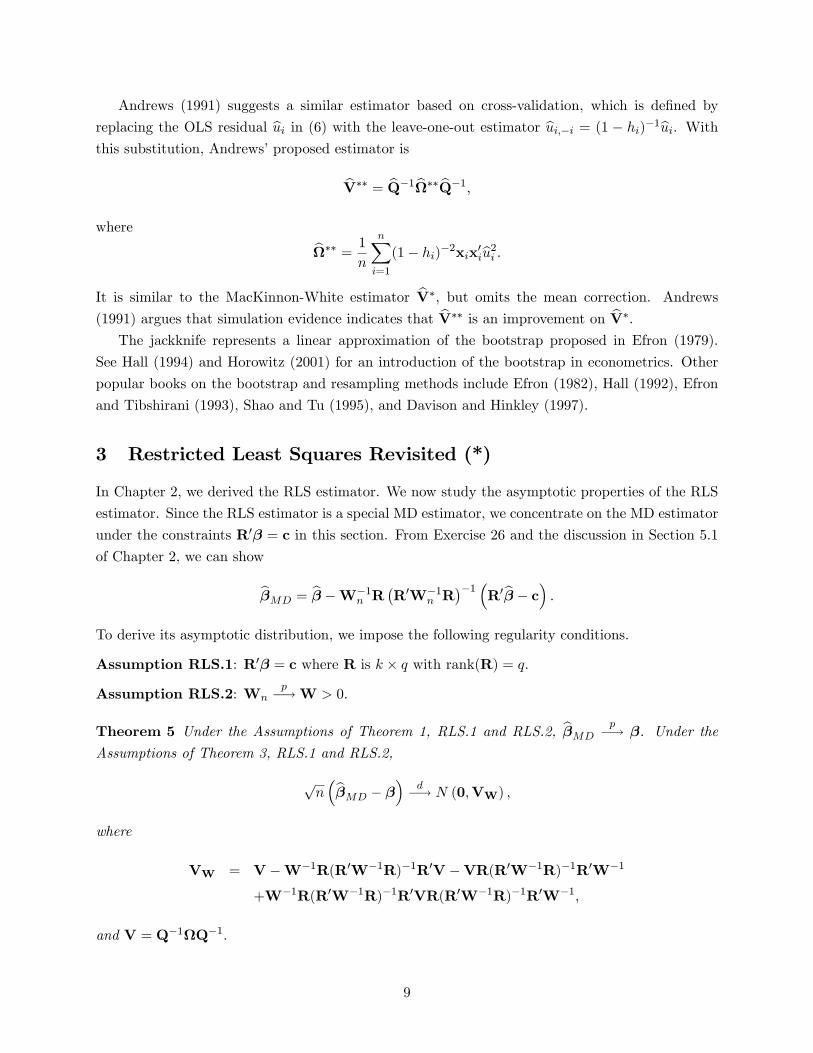
�b� � ��. Since bV� > 0, Cn is an ellipsoid in the � plane.To show Cn intuitively, assume q = 2 and � = (�1; �2)
0. In this case, Cn is an ellipse in the
(�1; �2) plane as shown in Figure 3. In Figure 3, we also show the (1 � �) CIs for �1 and �2. Itis tempting to use the rectangular region, say C0n, as a con�dence region for (�1; �2). However,
7Di¤erent from t-tests, Wald tests are hard to apply for one-sided alernatives.
21
0
Figure 3: Con�dence Region for (�1; �2)
P ((�1; �2) 2 C0n) may not converge to 1� �. For example, suppose b�1 and b�2 are asymptoticallyindependent; then P ((�1; �2) 2 C0n)! (1� �)2 < (1� �).
Exercise 12 Show that when b�1 and b�2 are asymptotically independent, P ((�1; �2) 2 C0n) !(1� �)2.
10 Problems with Tests of Nonlinear Hypotheses
While the t test and Wald tests work well when the hypothesis is a linear restriction on �, they
can work quite poorly when the restrictions are nonlinear. This can be seen in a simple example
introduced by Lafontaine and White (1986). Take the model
yi = � + ui; ui � N(0; �2)
and consider the hypothesis
H0: � = 1:
Let b� and b�2 be the sample mean and variance of yi. The standard Wald test for H0 isWn = n
�b� � 1�2b�2 :
22

1 2 3 4 5 6 7 8 9 100
0.5
1
1.5
2
2.5
3
3.5
4
4.5
Figure 4: Wald Statistic as a function of s
Now notice that H0 is equivalent to the hypothesis
H0(s): �s = 1;
for any positive integer s. Letting r(�) = �s, and noting R = s�s�1, we �nd that the standard
Wald test for H0(s) is
Wn(s) = n
�b�s � 1�2b�2s2b�2s�2 :
While the hypothesis �s = 1 is una¤ected by the choice of s, the statistic Wn(s) varies with s. This
is an unfortunate feature of the Wald statistic.
To demonstrate this e¤ect, we plot in Figure 4 the Wald statistic Wn(s) as a function of s,
setting n=b�2 = 10. The increasing solid line is for the case b� = 0:8 and the decreasing dashed lineis for the case b� = 1:6. It is easy to see that in each case there are values of s for which the teststatistic is signi�cant relative to asymptotic critical values, while there are other values of s for
which the test statistic is insigni�cant.8 This is distressing since the choice of s is arbitrary and
irrelevant to the actual hypothesis.
Our �rst-order asymptotic theory is not useful to help pick s, asWn(s)d�! �21 under H0 for any
s. This is a context where Monte Carlo simulation can be quite useful as a tool to study andcompare the exact distributions of statistical procedures in �nite samples. The method uses random
simulation to create arti�cial datasets, to which we apply the statistical tools of interest. This
8Breusch and Schmidt (1988) show that any positive value for the Wald test statistic is possible by rewriting H0
in an algebraically equivalent form.
23

produces random draws from the statistic�s sampling distribution. Through repetition, features
of this distribution can be calculated. In the present context of the Wald statistic, one feature
of importance is the Type I error of the test using the asymptotic 5% critical value 3:84 - the
probability of a false rejection, P (Wn(s) > 3:84j� = 1). Given the simplicity of the model, this
probability depends only on s, n, and �2. In Table 1 we report the results of a Monte Carlo
simulation where we vary these three parameters: the value of s is varied from 1 to 10, n is varied
among 20, 100 and 500, and � is varied among 1 and 3. The table reports the simulation estimate
of the Type I error probability from 50; 000 random samples. Each row of the table corresponds
to a di¤erent value of s - and thus corresponds to a particular choice of test statistic. The second
through seventh columns contain the Type I error probabilities for di¤erent combinations of n and
�. These probabilities are calculated as the percentage of the 50; 000 simulated Wald statistics
Wn(s) which are larger than 3:84. The null hypothesis �s = 1 is true, so these probabilities are
Type I error.
� = 1 � = 3
s n = 20 n = 100 n = 500 n = 20 n = 100 n = 500
1 .06 .05 .05 .07 .05 .05
2 .08 .06 .05 .15 .08 .06
3 .10 .06 .05 .21 .12 .07
4 .13 .07 .06 .25 .15 .08
5 .15 .08 .06 .28 .18 .10
6 .17 .09 .06 .30 .20 .11
7 .19 .10 .06 .31 .22 .13
8 .20 .12 .07 .33 .24 .14
9 .22 .13 .07 .34 .25 .15
10 .23 .14 .08 .35 .26 .16
Table 1: Type I Error Probability of Asymptotic 5% Wn(s) Test
Note: Rejection frequencies from 50,000 simulated random samples
To interpret the table, remember that the ideal Type I error probability is 5%(:05) with devia-
tions indicating distortion. Type I error rates between 3% and 8% are considered reasonable. Error
rates above 10% are considered excessive. Rates above 20% are unacceptable. When comparing
statistical procedures, we compare the rates row by row, looking for tests for which rejection rates
are close to 5% and rarely fall outside of the 3%� 8% range. For this particular example the only
test which meets this criterion is the conventional Wn = Wn(1) test. Any other choice of s leads
to a test with unacceptable Type I error probabilities.
In Table 1 you can also see the impact of variation in sample size. In each case, the Type I
error probability improves towards 5% as the sample size n increases. There is, however, no magic
choice of n for which all tests perform uniformly well. Test performance deteriorates as s increases,
which is not surprising given the dependence of Wn(s) on s as shown in Figure 4.
24

In this example it is not surprising that the choice s = 1 yields the best test statistic. Other
choices are arbitrary and would not be used in practice. While this is clear in this particular
example, in other examples natural choices are not always obvious and the best choices may in fact
appear counter-intuitive at �rst. This point can be illustrated through another example which is
similar to one developed in Gregory and Veall (1985). Take the model
yi = �0 + x1i�1 + x2i�2 + ui; E[xiui] = 0 (19)
and the hypothesis
H0:�1�2= �0
where �0 is a known constant. Equivalently, de�ne � = �1=�2, so the hypothesis can be stated as
H0: � = �0. Let b� = �b�0; b�1; b�2�0 be the least-squares estimates of (19), bVb� be an estimate of thecovariance matrix for b� and b� = b�1=b�2.9 De�ne
bR1 = 0; 1b�2 ;�b�1b�22!0
so that the standard error for b� is s(b�) = �bR01 bV bR1�1=2. In this case, a t-statistic for H0 ist1n =
b�1=b�2 � �0s(b�) :
An alternative statistic can be constructed through reformulating the null hypothesis as
H0: �1 � �0�2 = 0:
A t-statistic based on this formulation of the hypothesis is
t2n =b�1 � �0b�2�R02bVb�R2
�1=2 ;where R2 = (0; 1;��0)0.
To compare t1n and t2n we perform another simple Monte Carlo simulation. We let x1i and
x2i be mutually independent N(0; 1) variables, ui be an independent N(0; �2) draw with � = 3,
and normalize �0 = 1 and �1 = 1. This leaves �2 as a free parameter, along with sample size n.
We vary �2 among :1; :25; :50; :75; and 1:0 and n among 100 and 500. The one-sided Type I error
probabilities P (tn < �1:645) and P (tn > 1:645) are calculated from 50; 000 simulated samples.
The results are presented in Table 2. Ideally, the entries in the table should be 0:05. However,
the rejection rates for the t1n statistic diverge greatly from this value, especially for small values of
9 If bV is used to estimate the asymptotic variance ofpn�b� � ��, then bVb� = bV=n.
25

�2. The left tail probabilities P (t1n < �1:645) greatly exceed 5%, while the right tail probabilitiesP (t1n > 1:645) are close to zero in most cases. In contrast, the rejection rates for the linear t2nstatistic are invariant to the value of �2, and are close to the ideal 5% rate for both sample sizes.
The implication of Table 2 is that the two t-ratios have dramatically di¤erent sampling behaviors.
n = 100 n = 500
P (tn < �1:645) P (tn > 1:645) P (tn > 1:645) P (tn > 1:645)
�2 t1n t2n t1n t2n t1n t2n t1n t2n
.10 .47 .06 .00 .06 .28 .05 .00 .05
.25 .26 .06 .00 .06 .15 .05 .00 .05
.50 .15 .06 .00 .06 .10 .05 .00 .05
.75 .12 .06 .00 .06 .09 .05 .00 .05
1.00 .10 .06 .00 .06 .07 .05 .02 .05
Table 2: Type I Error Probability of Asymptotic 5% t-tests
The common message from both examples is that Wald statistics are sensitive to the algebraic
formulation of the null hypothesis. In all cases, if the hypothesis can be expressed as a linear
restriction on the model parameters, this formulation should be used. If no linear formulation
is feasible, then the "most linear" formulation should be selected (as suggested by the theory of
Phillips and Park (1988)), and alternatives to asymptotic critical values should be considered. It
is also prudent to consider alternative tests to the Wald statistic, such as the minimum distance
statistic developed in the next section.
11 Minimum Distance Test (*)
The likelihood ratio (LR) test is valid only under homoskedasticity. The counterpart of the LR
test in the heteroskedastic environment is the minimum distance test. Based on the idea of the LR
test, the minimum distance statistic is de�ned as
Jn = minr(�)=0
Jn (�)�min�Jn (�) = min
r(�)=0Jn
�b�MD
�;
where min�Jn (�) = 0 if no restrictions are imposed (why?). Jn � 0 measures the cost (on Jn (�))
of imposing the null restriction r(�) = 0. Usually,Wn in Jn(�) is chosen to be the e¢ cient weight
matrix bV�1, and the corresponding Jn is denoted as J�n with
J�n = n�b� � b�EMD
�0 bV�1�b� � b�EMD
�:
Consider the class of linear hypotheses H0: R0� = c. In this case, we know from (9) that
b� � b�MD = bVR�R0 bVR��1 �R0b� � c� ;26

so
J�n = n�R0b� � c�0 �R0 bVR��1R0 bV bV�1 bVR�R0 bVR��1 �R0b� � c�
= n�R0b� � c�0 �R0 bVR��1 �R0b� � c� =Wn:
Thus for linear hypotheses, the e¢ cient minimum distance statistic J�n is identical to the Wald
statstic Wn which is heteroskedastic-robust.
Exercise 13 Show that J�n =W under homoskedasticity when the null hypothesis is H0: R0� = c,
where W is the homoskedastic form of the Wald statistic de�ned in Chapter 4.
For nonlinear hypotheses, however, the Wald and minimum distance statistics are di¤erent.
We know from Section 10 that the Wald statistic is not robust to the formulation of the null
hypothesis. However, like the LR test statistic, the minimum distance statistic is invariant to
the algebraic formulation of the null hypothesis, so is immune to this problem. Consequently, a
simple solution to the problem associated with Wn in Section 10 is to use the minimum distance
statistic Jn, which equalsWn with s = 1 in the �rst example, and jt2nj in the second example there.Whenever possible, the Wald statistic should not be used to test nonlinear hypotheses.
Exercise 14 Show that J�n = Wn(1) in the �rst example and J�n = t22n in the second example of
Section 10.
Newey and West (1987a) established the asymptotic null distribution of J�n for linear and non-
linear hypotheses.
Theorem 11 Under the assumptions of Theorem 8, J�nd�! �2q under H0.
12 The Heteroskedasticity-Robust LM Test (*)
The validity of the LM test in the normal regression model depends on the assumption that the
error is homoskedastic. In this section, we extend the homoskedasticity-only LM test to the
heteroskedasticity-robust form. Suppose the null hypothesis is H0: �2 = 0, where � is decom-
posed as (�01;�02)0, �1 and �2 are k1 � 1 and k2 � 1 vectors, respectively, k = k1 + k2, and x is
decomposed as (x01;x02)0 correspondingly with x1 including the constant.
Exercise 15 Show that testing any linear constraints R0� = c is equivalent to testing some originalcoe¢ cients being zero in a new regression with rede�ned X and y, where R 2 Rk2�k is full rank.
After some algebra we can write
LM =
n�1=2
nXi=1
brieui!0 e�2n�1 nXi=1
bribr0i!�1
n�1=2nXi=1
brieui! ;27

where e�2 = n�1Pni=1 eu2i and each bri is a k2 � 1 vector of OLS residuals from the (multivariate)
regression of xi2 on xi1, i = 1; � � � ; n. This statistic is not robust to heteroskedasticity because thematrix in the middle is not a consistent estimator of the asymptotic variance of n�1=2
Pni=1 brieui
under heteroskedasticity. A heteroskedasticity-robust statistic is
LMn =
n�1=2
nXi=1
brieui!0 n�1 nXi=1
eu2ibribr0i!�1
n�1=2nXi=1
brieui!
=
nXi=1
brieui!0 nXi=1
eu2ibribr0i!�1 nX
i=1
brieui! :Dropping the i subscript, this is easily obtained as n � SSR0 from the OLS regression (without
intercept)10
1 on eu � br; (20)
where eu � br = (eu � br1; � � � ; eu � brk2)0 is the k2 � 1 vector obtained by multiplying eu by each elementof br and SSR0 is just the usual sum of squared residuals from the regression. Thus, we �rst
regress each element of x2 onto all of x1 and collect the residuals in br. Then we form eu � br(observation by observation) and run the regression in (20); n � SSR0 from this regression is
distributed asymptotically as �2k2 . For more details, see Davidson and MacKinnon (1985, 1993) or
Wooldridge (1991, 1995).
13 Test Consistency
We now de�ne the test consistency against �xed alternatives. This concept was �rst introduced by
Wald and Wolfowitz (1940).
De�nition 1 A test of H0: � 2 �0 is consistent against �xed alternatives if for all � 2 �1,
P (Reject H0j�)! 1 as n!1.
To understand this concept, consider the following simple example. Suppose that yi is i.i.d. N(�; 1).
Consider the t-statistic tn(�) =pn (y � �), and tests of H0: � = 0 against H1: � > 0. We reject
H0 if tn = tn(0) > c. Note that
tn = tn (�) +pn�
and tn(�) � Z has an exact N(0; 1) distribution. This is because tn (�) is centered at the true
mean �, while the test statistic tn(0) is centered at the (false) hypothesized mean of 0. The power
of the test is
P (tn > cj�) = P�Z +
pn� > c
�= 1� �
�c�
pn��:
This function is monotonically increasing in � and n, and decreasing in c. Notice that for any c
and � 6= 0, the power increases to 1 as n!1. This means that for � 2 H1, the test will reject H010 If there is an intercept, then the regression is trivial.
28

with probability approaching 1 as the sample size gets large. This is exactly test consistency.
For tests of the form �Reject H0 if Tn > c�, a su¢ cient condition for test consistency is that
Tn diverges to positive in�nity with probability one for all � 2 �1. In general, the t-test and Waldtest are consistent against �xed alternatives. For example, in testing H0: � = �0,
tn =b� � �0s�b�� =
b� � �s�b�� +
pn (� � �0)qbV� (21)
since s�b�� = qbV�=n. The �rst term on the right-hand-side converges in distribution to N(0; 1).
The second term on the right-hand-side equals zero if � = �0, converges in probability to +1 if
� > �0, and converges in probability to �1 if � < �0. Thus the two-sided t-test is consistent
against H1: � 6= �0, and one-sided t-tests are consistent against the alternatives for which they aredesigned. For another example, The Wald statistic for H0: � = r(�) = �0 against H1: � 6= �0 is
Wn = n�b� � �0�0 bV�1
�
�b� � �0� :Under H1, b� p�! � 6= �0. Thus
�b� � �0�0 bV�1�
�b� � �0� p�! (� � �0)0V�1� (� � �0) > 0. Hence
under H1, Wnp�!1. Again, this implies that Wald tests are consistent tests.
(*) Andrews (1986) introduces a testing analogue of estimator consistency, called completeconsistency, which he shows is more appropriate than test consistency. It is shown that a sequenceof estimators is consistent, if and only if certain tests based on the estimators (such as Wald or
likelihood ratio tests) are completely consistent, for all simple null hypotheses.
14 Asymptotic Local Power
Consistency is a good property for a test, but does not give a useful approximation to the power of
a test. To approximate the power function we need a distributional approximation. The standard
asymptotic method for power analysis uses what are called local alternatives. This is similarto our analysis of restriction estimation under misspeci�cation. The technique is to index the
parameter by sample size so that the asymptotic distribution of the statistic is continuous in a
localizing parameter. We �rst consider the t-test and then the Wald test.
In the t-test, we consider parameter vectors �n which are indexed by sample size n and satisfy
the real-valued relationship
�n = r(�n) = �0 + n�1=2h, (22)
where the scalar h is called a localizing parameter. We index �n and �n by sample size toindicate their dependence on n. The way to think of (22) is that the true value of the parameters
are �n and �n. The parameter �n is close to the hypothesized value �0, with deviation n�1=2h. Such
a sequence of local alternatives �n is often called a Pitman (1949) drift or a Pitman sequence.11
11See McManus (1991) for who invented local power analysis.
29

We know for a �xed alternative, the power will converge to 1 as n ! 1. To o¤set the e¤ect ofincreasing n, we make the alternative harder to distinguish from H0 as n gets larger. The rate
n�1=2 is the correct balance between these two forces. In the statistical literature, such alternatives
are termed as "contiguous" local alternatives.
The speci�cation (22) states that for any �xed h, �n approaches �0 as n gets large. Thus �nis �close� or �local� to �0. The concept of a localizing sequence (22) might seem odd at �rst as
in the actual world the sample size cannot mechanically a¤ect the value of the parameter. Thus
(22) should not be interpreted literally. Instead, it should be interpreted as a technical device
which allows the asymptotic distribution of the test statistic to be continuous in the alternative
hypothesis.
Similarly as in (21),
tn =b� � �0s�b�� =
b� � �ns�b�� +
pn (�n � �0)qbV�
d�! Z + �
under the local alternative (22), where Z � N(0; 1) and � = h=pV�. In testing the one-sided
alternative H1: � > �0, a t-test rejects H0 for tn > z�. The asymptotic local power of this testis the limit of the rejection probability under the local alternative (22),
limn!1
P (Reject H0j� = �n) = limn!1
P (tn > z�j� = �n)= P (Z + � > z�) = 1� �(z� � �) = �(� � z�) � �� (�) :
We call �� (�) the local power function.
Exercise 16 Derive the local power function for the two-sided t-test.
In Figure 5 we plot the local power function �� (�) as a function of � 2 [0; 4] for tests of
asymptotic size � = 0:10; � = 0:50, and � = 0:01. We do not consider � < 0 since �n should be
greater than �0. � = 0 corresponds to the null hypothesis so �� (0) = �. The power functions
are monotonically increasing in both � and �. The monotonicity with respect to � is due to the
inherent trade-o¤ between size and power. Decreasing size induces a decrease in power, and vice
versa. The coe¢ cient � can be interpreted as the parameter deviation measured as a multiple of
the standard error s�b��. To see this, recall that s�b�� = n�1=2
qbV� � n�1=2pV� and then note
that
� =hpV�� n�1=2h
s�b�� =
�n � �0s�b�� ;
meaning that � equals the deviation �n � �0 expressed as multiples of the standard error s�b��.
Thus as we examine Figure 5, we can interpret the power function at � = 1 (e.g., 26% for a 5% size
test) as the power when the parameter �n is one standard error above the hypothesized value.
30

0 1 1.29 1.65 2.33 40.010.05
0.1
0.26
0.39
0.5
1
Figure 5: Asymptotic Local Power Function of One-Sided t-Test
Exercise 17 Suppose we have n0 data points, and we want to know the power when the true valueof � is #. Which � we should confer in Figure 5?
The di¤erence between power functions can be measured either vertically or horizontally. For
example, in Figure 5 there is a vertical dotted line at � = 1, showing that the asymptotic local
power �� (1) equals 39% for � = 0:10, equals 26% for � = 0:05 and equals 9% for � = 0:01.
This is the di¤erence in power across tests of di¤ering sizes, holding �xed the parameter in the
alternative. A horizontal comparison can also be illuminating. To illustrate, in Figure 5 there is
a horizontal dotted line at 50% power. 50% power is a useful benchmark, as it is the point where
the test has equal odds of rejection and acceptance. The dotted line crosses the three power curves
at � = 1:29 (� = 0:10), � = 1:65 (� = 0:05), and � = 2:33 (� = 0:01). This means that the
parameter � must be at least 1:65 standard errors above the hypothesized value for the one-sided
test to have 50% (approximate) power. The ratio of these values (e.g., 1:65=1:29 = 1:28 for the
asymptotic 5% versus 10% tests) measures the relative parameter magnitude needed to achieve the
same power. (Thus, for a 5% size test to achieve 50% power, the parameter must be 28% larger
than for a 10% size test.) Even more interesting, the square of this ratio (e.g., (1:65=1:29)2 = 1:64)
can be interpreted as the increase in sample size needed to achieve the same power under �xed
parameters. That is, to achieve 50% power, a 5% size test needs 64% more observations than
a 10% size test. This interpretation follows by the following informal argument. By de�nition
and (22) � = h=pV� =
pn (�n � �0) =
pV�. Thus holding � and V� �xed, we can see that �2 is
proportional to n.
We next generalize the local power analysis to the case of vector-valued alternatives. Now the
31

local parametrization takes the form
�n = r(�n) = �0 + n�1=2h; (23)
where h is a q � 1 vector. Under (23),
pn�b� � �0� = pn�b� � �n�+ h d�! Zh � N(h;V�);
a normal random vector with mean h and variance matrix V�. Applied to the Wald statistic we
�nd
Wn = n�b� � �0�0 bV�1
�
�b� � �0� d�! Z0hV�1� Zh � �
2q(�):
where �2q(�) is a non-central chi-square distribution with q degrees of freedom and non-centralparameter (or noncentrality) � = h0V�1
� h. Under the null, h = 0, and the �2q(�) distribution then
degenerates to the usual �2q distribution. In the case of q = 1, jZ + �j2 � �21(�) with � = �2. The
asymptotic local power of the Wald test at the level � is
P��2q(�) > �
2q;�
�� �q;� (�) :
Figure 6 plots �q;:05 (�) (the power of asymptotic 5% tests) as a function of � for q = 1, 2 and 3.
The power functions are monotonically increasing in � and asymptote to one. Figure 6 also shows
the power loss for �xed non-centrality parameter � as the dimensionality of the test increases. The
power curves shift to the right as q increases, resulting in a decrease in power. This is illustrated by
the dotted line at 50% power. The dotted line crosses the three power curves at � = 3:85 (q = 1),
� = 4:96 (q = 2), and � = 5:77 (q = 3). The ratio of these � values correspond to the relative
sample sizes needed to obtain the same power. Thus increasing the dimension of the test from
q = 1 to q = 2 requires a 28% increase in sample size, or an increase from q = 1 to q = 3 requires
a 50% increase in sample size, to obtain a test with 50% power. Intuitively, when testing more
restrictions, we need more deviation from the null (or equivalently, more data points) to achieve
the same power.
Exercise 18 (i) Show that bV� p�! V� under the local alternative �n = �0 + n�1=2b. (ii) If the
local alternative �n is speci�ed as as in (i), what is the local power?
Exercise 19 (*) Derive the local power function of the minimum distance test with local alterna-
tives (23). Is it the same as the Wald test?
Exercise 20 (Empirical) The data set invest.dat contains data on 565 U.S. �rms extracted fromCompustat for the year 1987. The variables, in order, are
� Ii Investment to Capital Ratio (multiplied by 100).
� Qi Total Market Value to Asset Ratio (Tobin�s Q).
32

0 3.85 4.96 5.77 160
0.05
0.5
1
Figure 6: Asymptotic Local Power Function of the Wald Test
� Ci Cash Flow to Asset Ratio.
� Di Long Term Debt to Asset Ratio.
The �ow variables are annual sums for 1987. The stock variables are beginning of year.
(a) Estimate a linear regression of Ii on the other variables. Calculate appropriate standard errors.
(b) Calculate asymptotic con�dence intervals for the coe¢ cients.
(c) This regression is related to Tobin�s q theory of investment, which suggests that investmentshould be predicted solely by Qi. Thus the coe¢ cient on Qi should be positive and the others
should be zero. Test the joint hypothesis that the coe¢ cients on Ci and Di are zero. Test the
hypothesis that the coe¢ cient on Qi is zero. Are the results consistent with the predictions of
the theory?
(d) Now try a non-linear (quadratic) speci�cation. Regress Ii on Qi, Ci, Di, Q2i , C2i , D
2i , QiCi,
QiDi, CiDi. Test the joint hypothesis that the six interaction and quadratic coe¢ cients are
zero.
Exercise 21 (Empirical) In a paper in 1963, Marc Nerlove analyzed a cost function for 145American electric companies. The data �le nerlov.dat contains his data. The variables are described
as follows,
� Column 1: total costs (call it TC) in millions of dollars
33

� Column 2: output (Q) in billions of kilowatt hours
� Column 3: price of labor (PL)
� Column 4: price of fuels (PF)
� Column 5: price of capital (PK)
Nerlove was interested in estimating a cost function: TC = f(Q;PL; PF; PK).
(a) First estimate an unrestricted Cobb-Douglas speci�cation
log TCi = �1 + �2 logQi + �3 logPLi + �4 logPKi + �5 logPFi + ui: (24)
Report parameter estimates and standard errors.
(b) Using a Wald statistic, test the hypothesis H0: �3 + �4 + �5 = 1.
(c) Estimate (24) by least-squares imposing this restriction by substitution. Report your parameterestimates and standard errors.
(d) Estimate (24) subject to �3 + �4 + �5 = 1 using the RLS estimator. Do you obtain the sameestimates as in part (c)?
Technical Appendix: Expected Length of a Con�dence Interval
Suppose L � � � U is a CI for �, where L and U are random. The expected length of the interval
is E[U � L], which turns out equal toZ� 6=�0
P (L � � � U) d�;
the integrated probability of the interval covering the false value, where P (�) is the probabilitymeasure under the truth �0. To see why, note that
E[U � L] =
Z Z1 (L � � � U) d�dP
=
Z Z1 (L � � � U) dPd�
=
ZP (L � � � U) d� =
Z� 6=�0
P (L � � � U) d�:
So minimizing the expected length of a CI is equivalent to minimizing the coverage probability for
each � 6= �0. From the discussion in the main text,
P (L � � � U) = P (X 2 A (�)) ;
34

where X is the data and A (�) is the acceptance region for the null that � is the true value. As a
result, for � 6= �0, P (L � � � U) is the type II error in testing H0 : � vs H1 : �0, and minimizingP (L � � � U) is equivalent to maximizing the power. By the Neyman-Pearson Lemma, the mostpowerful test is
1
�f(X)
f�(X)> c(�)
�; (25)
where f(X) is the true density of X (or density under �0), and c(�) is the critical value for H0 : �.
Collecting all ��s such that f(X)f�(X)
� c(�) is the length minimizing CI.The arguments above assume �0 were known, but if it were known, why do we need a CI for it?
A more natural measure for the interval length is the average expected lengthRE# [U � L] d� (#),
where # is the parameter in the model and � (�) is a measure for # representing some prior infor-mation. Similarly, we can showZ
E# [U � L] d� (#) =Z Z
P# (X 2 A (�)) d� (#) d�:
Minimizing the average expected length is equivalent to maximizing the power in testing H0 : � vs
H1 : P (�), where P (X 2 A) =RP# (X 2 A) d� (#) has the density
Rf#(X)d� (#) with f#(�) being
the density associated with P#(�). For any test ', the average powerZE# ['] d� (#) =
Z Z'f#(X)dXd� (#) =
Z'
Zf#(X)d� (#) dX =
Z'dP (X)
is just the power in the above test, so the test maximizing the power against P (�) is equivalentto maximizing the average power
RE# ['] d� (#). The corresponding test is the same as (25) but
replaces f(X) byRf#(X)d� (#).
35
Related Documents