1 Chapter 5: Forecasting Textbook: pp. 165-202 Every day, managers make decisions without knowing what will happen in the future …

Welcome message from author
This document is posted to help you gain knowledge. Please leave a comment to let me know what you think about it! Share it to your friends and learn new things together.
Transcript

1
Chapter 5: Forecasting
Textbook: pp. 165-202
Every day, managers make
decisions without knowing what will
happen in the future …
2
Learning Objectives
After completing this chapter, students will be able to:
• Understand and know when to use various families of
forecasting models
• Compare moving averages, exponential smoothing, and
other time-series models
• Calculate measures of forecast accuracy
• Apply forecast models for random variations
• Apply forecast models for trends and random variations
• Manipulate data to account for seasonal variations
• Apply forecast models for trends, seasonal variations, and
random variations
• Explain how to monitor and control forecasts

3
Main purpose of forecasting:
Managers are trying to reduce uncertainty and
make better estimates of what will happen in the
future!
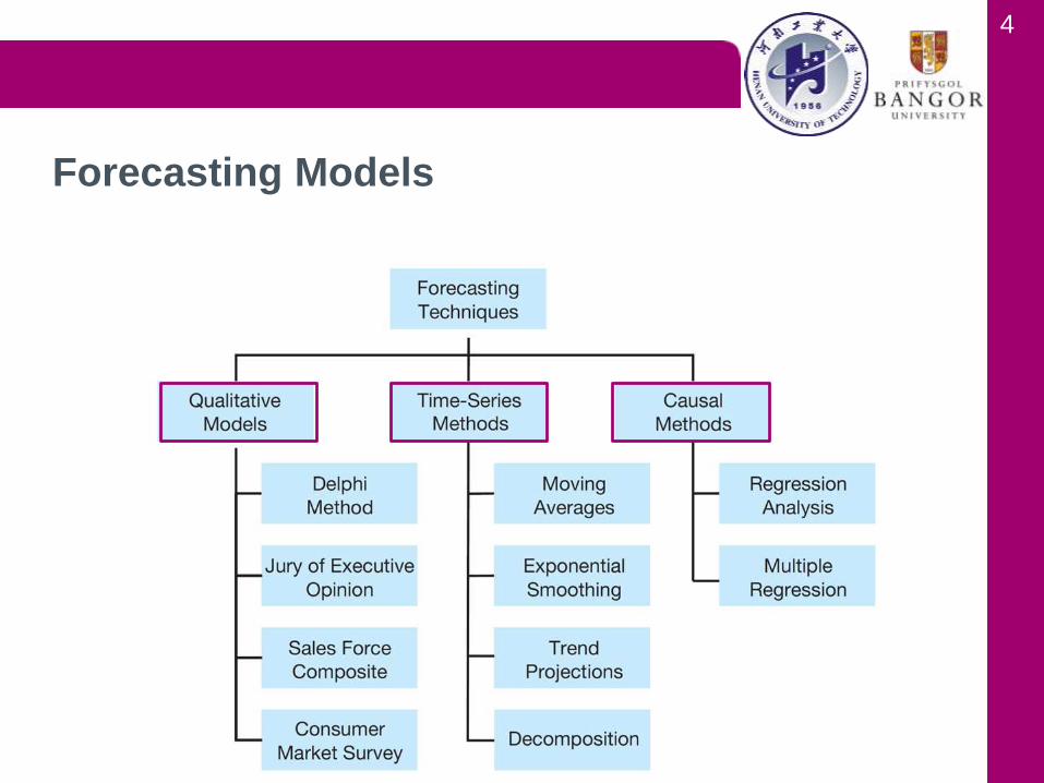
• Subjective methods
“Seat-of-the pants methods” - intuition, experience
• More formal quantitative (e.g. least squares regression
analysis, trend projections …) and qualitative
techniques
Introduction
4
Forecasting Models
5
• Incorporate judgmental or subjective factors
o Useful when subjective factors are important or
accurate quantitative data is difficult to obtain
• Common qualitative techniques
1. Delphi method
2. Jury of executive opinion
3. Sales force composite
4. Consumer market surveys
Qualitative Models (1 of 3)
6
• Delphi Method
o Iterative group process
o Respondents provide input to decision makers
o Repeated until consensus is reached
• Jury of Executive Opinion
o Collects opinions of a small group of high-level
managers
o May use statistical models for analysis
Qualitative Models (2 of 3)

7
• Sales Force Composite
o Allows individual salespersons estimates
o Reviewed for reasonableness
o Data is compiled at a district or national level
• Consumer Market Survey
o Information on purchasing plans solicited from
customers or potential customers
o Used in forecasting, product design, new product
planning
Qualitative Models (3 of 3)

8
• Predict the future based on the past
• Uses only historical data on one variable
• Extrapolations of past values of a series
Time-Series Models
• If we are forecasting weekly sales
for fidget spinners, we use the past
weekly sales for fidget spinners in
making the forecast for future sales
– ignoring other factors such as
the economy, competition, and
even the selling price of the fidget
spinners.
9
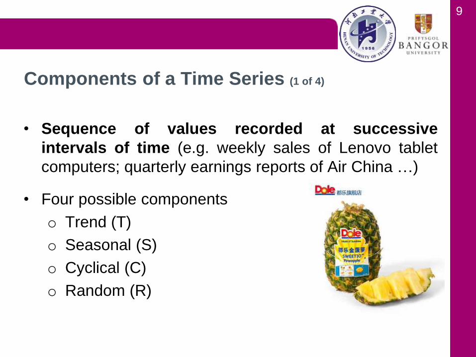
• Sequence of values recorded at successive
intervals of time (e.g. weekly sales of Lenovo tablet
computers; quarterly earnings reports of Air China …)
• Four possible components
o Trend (T)
o Seasonal (S)
o Cyclical (C)
o Random (R)
Components of a Time Series (1 of 4)
10
1. Trend (T) is the gradual upward or downward
movement of the data over time.
2. Seasonality (S) is a pattern of the demand
fluctuation above or below the trend line that
repeats at regular intervals.
3. Cycles (C) are patterns in annual data that occur
every several years. They are usually tied into the
business cycle (used only in very long forecasts!)
4. Random variations (R) are “blips” in the data
caused by chance and unusual situations; they
follow no discernible pattern.
Components of a Time Series (2 of 4)
11
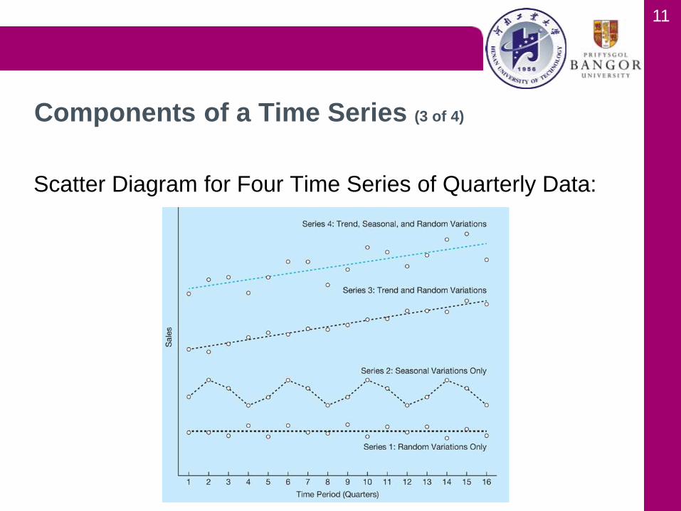
Scatter Diagram for Four Time Series of Quarterly Data:
Components of a Time Series (3 of 4)

12
Scatter Diagram of a Time Series with Cyclical and
Random Components:
Components of a Time Series (4 of 4)
13
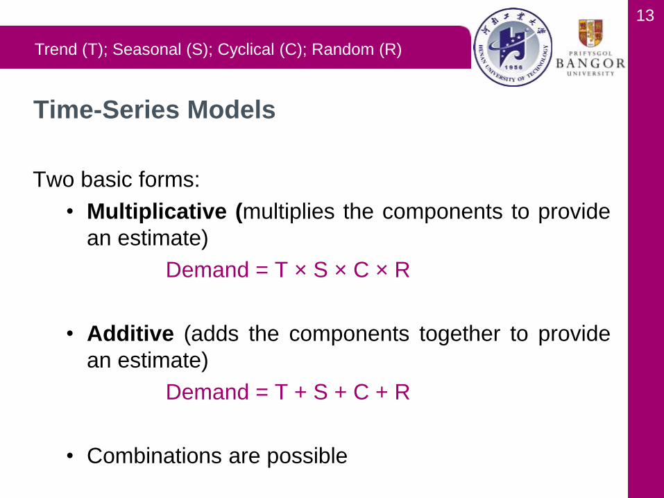
Two basic forms:
• Multiplicative (multiplies the components to provide
an estimate)
Demand = T × S × C × R
• Additive (adds the components together to provide
an estimate)
Demand = T + S + C + R
• Combinations are possible
Time-Series Models
Trend (T); Seasonal (S); Cyclical (C); Random (R)
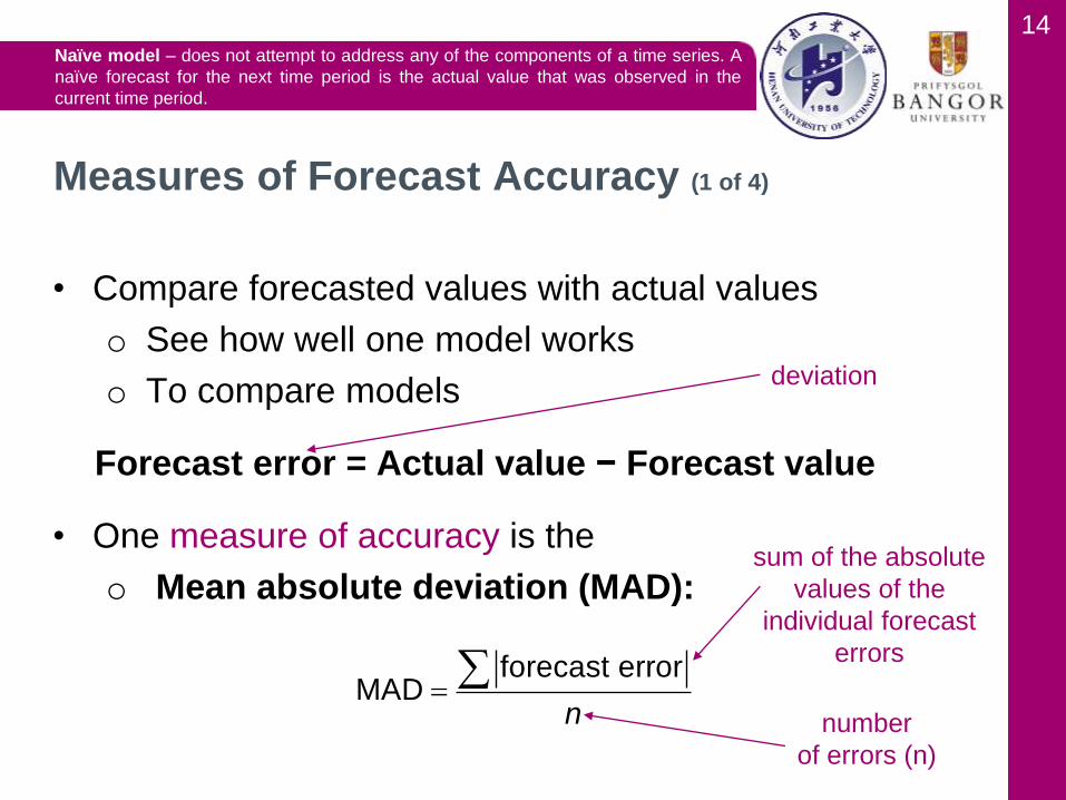
14
• Compare forecasted values with actual values
o See how well one model works
o To compare models
Forecast error = Actual value − Forecast value
• One measure of accuracy is the
o Mean absolute deviation (MAD):
Measures of Forecast Accuracy (1 of 4)
forecast errorMAD
n
deviation
sum of the absolute
values of the
individual forecast
errors
number
of errors (n)
Naïve model – does not attempt to address any of the components of a time series. A
naïve forecast for the next time period is the actual value that was observed in the
current time period.

15
Computing the Mean Absolute Deviation (MAD):
Measures of Forecast Accuracy (2 of 4)
forecast errorMAD
n
Absolute value |X| of a real number X is the non-negative value of X without
regard to its sign.
This means that – on average – each forecast missed the
actual value by 17.8 units!
16
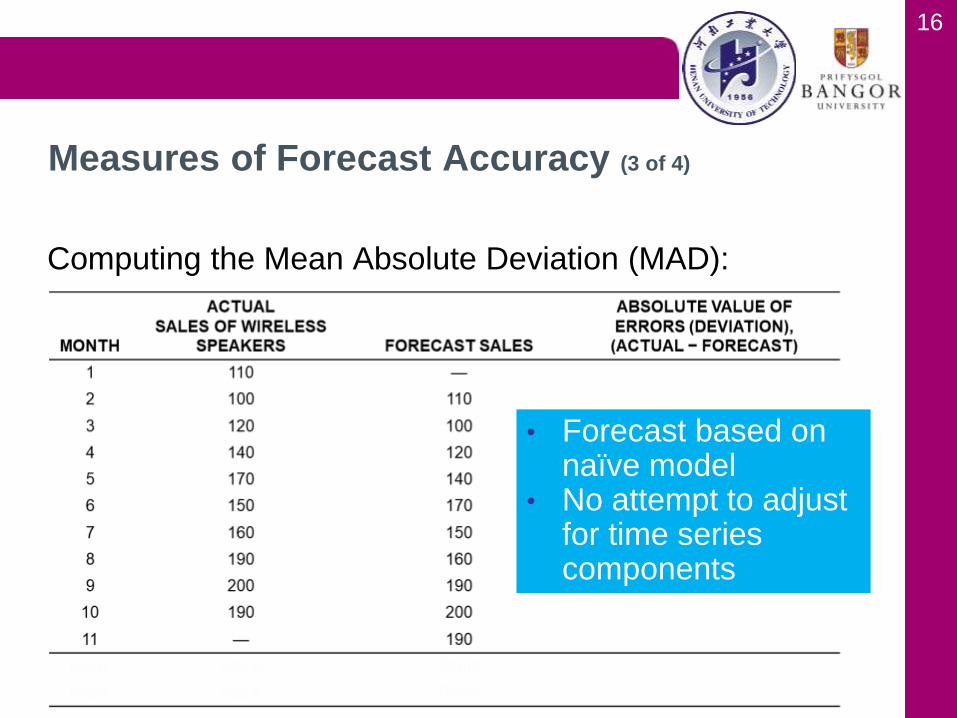
Computing the Mean Absolute Deviation (MAD):
Measures of Forecast Accuracy (3 of 4)
• Forecast based on naïve model
• No attempt to adjust for time series components
17
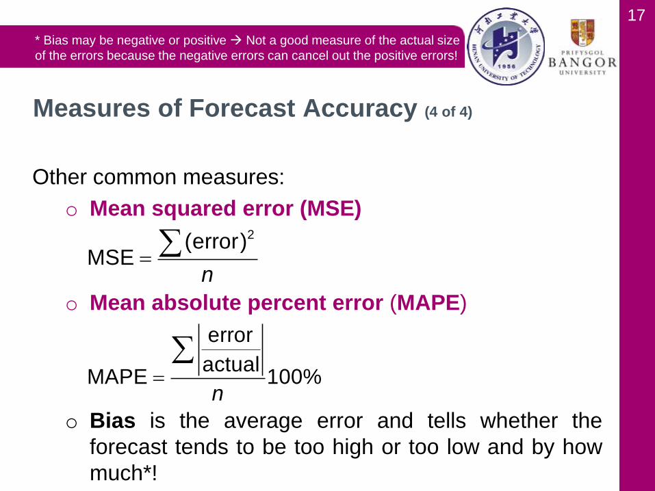
Other common measures:
o Mean squared error (MSE)
o Mean absolute percent error (MAPE)
o Bias is the average error and tells whether the
forecast tends to be too high or too low and by how
much*!
Measures of Forecast Accuracy (4 of 4)
2(error)MSE
n
error
actualMAPE 100%
n
* Bias may be negative or positive Not a good measure of the actual size
of the errors because the negative errors can cancel out the positive errors!
18
• If all variations in a time series are due to random
variations [no trend / seasonal / cyclical component is
present] some type of averaging or smoothing model
would be appropriate!
• Averaging techniques smooth out forecasts and will
not be too heavily influenced by random variations:
o Moving averages
o Weighted moving averages
o Exponential smoothing
Forecasting Random Variations
19
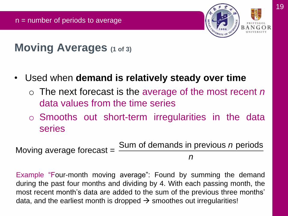
• Used when demand is relatively steady over time
o The next forecast is the average of the most recent n
data values from the time series
o Smooths out short-term irregularities in the data
series
Example “Four-month moving average”: Found by summing the demand
during the past four months and dividing by 4. With each passing month, the
most recent month’s data are added to the sum of the previous three months’
data, and the earliest month is dropped smoothes out irregularities!
Moving Averages (1 of 3)
Sum of demands in previous periodsMoving average forecast =
n
n
n = number of periods to average

20
Mathematically:
where Ft+1 = forecast for time period t + 1
Yt = actual value in time period t
n = number of periods to average
Moving Averages (2 of 3)
1 11
...t t t nt
Y Y YF
n
21
• Wallace Garden Supply wants to forecast demand for its
Storage Shed
o Collected data for the past year
o Use a three-month moving average (n = 3) and
forecast sales for the next January!
Wallace Garden Supply (1 of 4)
1 11
...t t t nt
Y Y YF
n
n = number of periods to average

22
Wallace Garden Supply --- Shed Sales (2 of 4)
1 11
...t t t nt
Y Y YF
n
n = number of periods to average
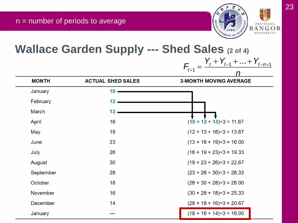
23
Wallace Garden Supply --- Shed Sales (2 of 4)
1 11
...t t t nt
Y Y YF
n
n = number of periods to average
24
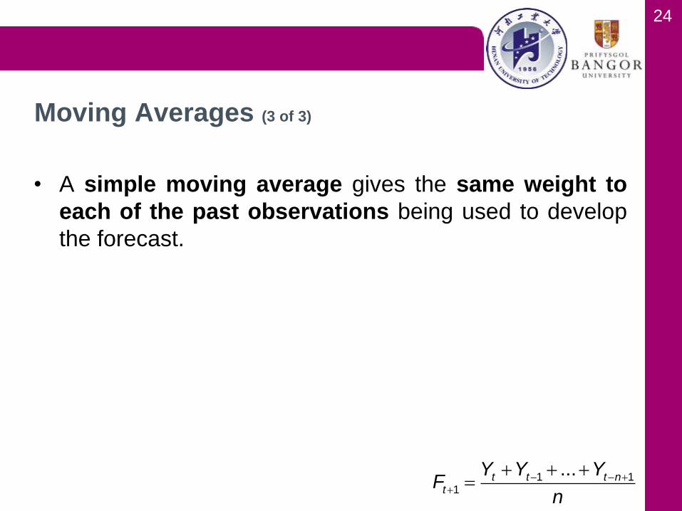
• A simple moving average gives the same weight to
each of the past observations being used to develop
the forecast.
Moving Averages (3 of 3)
1 11
...t t t nt
Y Y YF
n

25
• Weighted moving averages use weights to put more
emphasis on previous periods
• Often used when a trend or other pattern is emerging
Mathematically
where wi = weight for the ith observation
Weighted Moving Averages
1
(Weight in period )(Actual value in period )
(Weights)t
i iF
1 2 1 11
1 2
...
...t t n t n
t
n
w Y w Y w YF
w w w

26
• Use a 3-month weighted moving average model to
forecast demand
Weighting scheme:
Wallace Garden Supply (3 of 4)

27
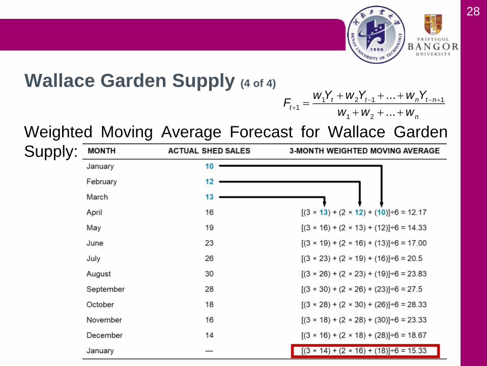
Weighted Moving Average Forecast for Wallace Garden
Supply:
Wallace Garden Supply (4 of 4)
1 2 1 11
1 2
...
...t t n t n
t
n
w Y w Y w YF
w w w
Weights of 3 for the most recent observation, 2 for the next observation,
and 1 for the most distant observation. The sum of weights is 6!
28
Weighted Moving Average Forecast for Wallace Garden
Supply:
Wallace Garden Supply (4 of 4)
1 2 1 11
1 2
...
...t t n t n
t
n
w Y w Y w YF
w w w

29
Exponential smoothing:
o A type of moving average
o Easy to use
o Requires little record keeping of data
New forecast = Last period’s forecast
+ α(Last period’s actual demand
− Last period’s forecast)
α is a weight (or smoothing constant) with a value 0 ≤ α ≤ 1
Exponential Smoothing (1 of 2)
30
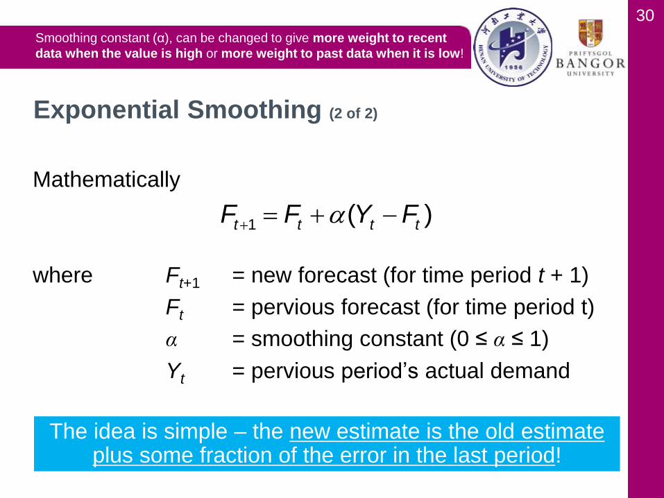
Mathematically
where Ft+1 = new forecast (for time period t + 1)
Ft = pervious forecast (for time period t)
α = smoothing constant (0 ≤ α ≤ 1)
Yt = pervious period’s actual demand
Exponential Smoothing (2 of 2)
1 ( )t t t tF F Y F
The idea is simple – the new estimate is the old estimate plus some fraction of the error in the last period!
Smoothing constant (α), can be changed to give more weight to recent
data when the value is high or more weight to past data when it is low!

31
• In January, February’s demand for a certain car model
was predicted to be 142
• Actual February demand was 153 autos
• Using a smoothing constant of α = 0.20, what is the
forecast for March?
New forecast (for March demand) =
Exponential Smoothing Example (1 of 2)
1 ( )t t t tF F Y F
Smoothing constant (α) is low --- more weight to past data is given.

32
• In January, February’s demand for a certain car model
was predicted to be 142
• Actual February demand was 153 autos
• Using a smoothing constant of α = 0.20, what is the
forecast for March?
New forecast (for March demand) = 142 + 0.2(153 − 142)
= 144.2 or 144 autos
If actual March demand = 136
New forecast (for April demand) =
Exponential Smoothing Example (1 of 2)
1 ( )t t t tF F Y F
33
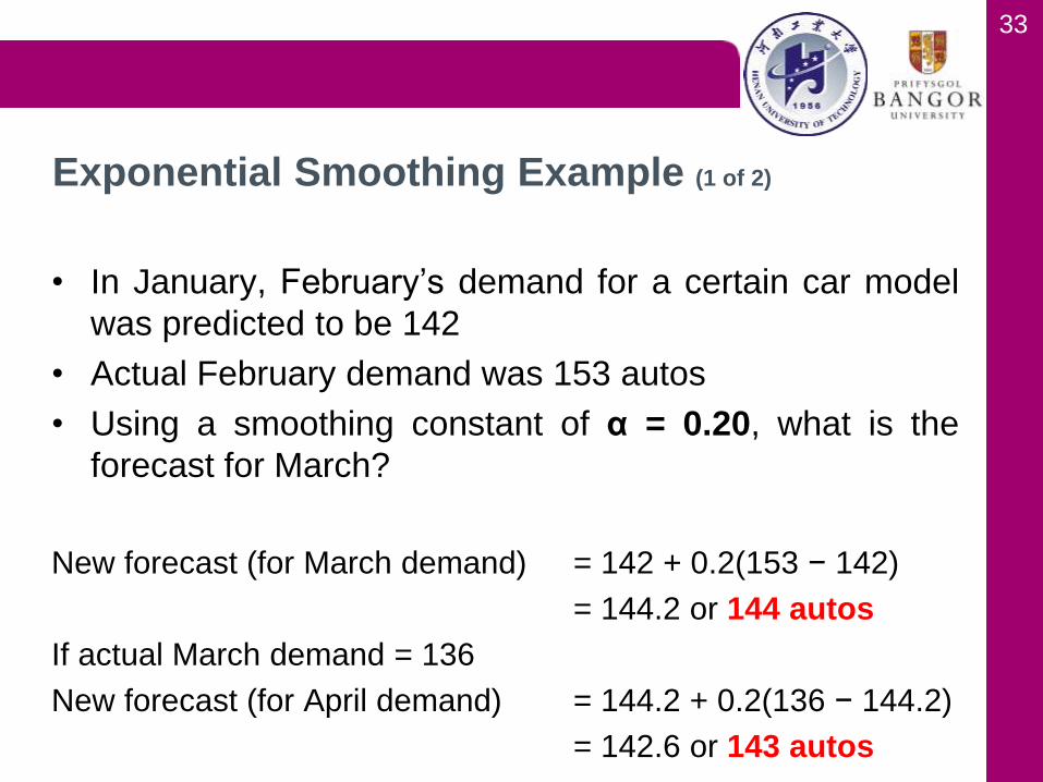
• In January, February’s demand for a certain car model
was predicted to be 142
• Actual February demand was 153 autos
• Using a smoothing constant of α = 0.20, what is the
forecast for March?
New forecast (for March demand) = 142 + 0.2(153 − 142)
= 144.2 or 144 autos
If actual March demand = 136
New forecast (for April demand) = 144.2 + 0.2(136 − 144.2)
= 142.6 or 143 autos
Exponential Smoothing Example (1 of 2)
34
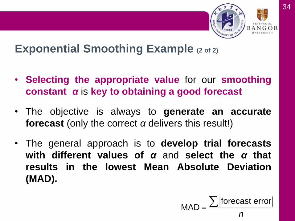
• Selecting the appropriate value for our smoothing
constant α is key to obtaining a good forecast
• The objective is always to generate an accurate
forecast (only the correct α delivers this result!)
• The general approach is to develop trial forecasts
with different values of α and select the α that
results in the lowest Mean Absolute Deviation
(MAD).
Exponential Smoothing Example (2 of 2)
forecast errorMAD
n
35
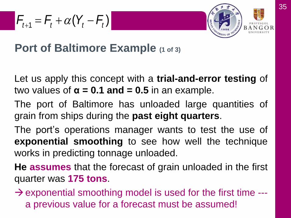
Let us apply this concept with a trial-and-error testing of
two values of α = 0.1 and = 0.5 in an example.
The port of Baltimore has unloaded large quantities of
grain from ships during the past eight quarters.
The port’s operations manager wants to test the use of
exponential smoothing to see how well the technique
works in predicting tonnage unloaded.
He assumes that the forecast of grain unloaded in the first
quarter was 175 tons.
exponential smoothing model is used for the first time ---
a previous value for a forecast must be assumed!
Port of Baltimore Example (1 of 3)
1 ( )t t t tF F Y F
36
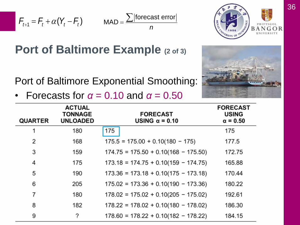
Port of Baltimore Exponential Smoothing:
• Forecasts for α = 0.10 and α = 0.50
Port of Baltimore Example (2 of 3)
1 ( )t t t tF F Y F
forecast errorMAD
n
37
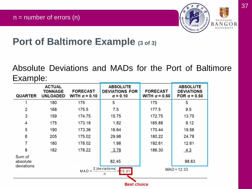
Absolute Deviations and MADs for the Port of Baltimore
Example:
Port of Baltimore Example (3 of 3)
n = number of errors (n)
38
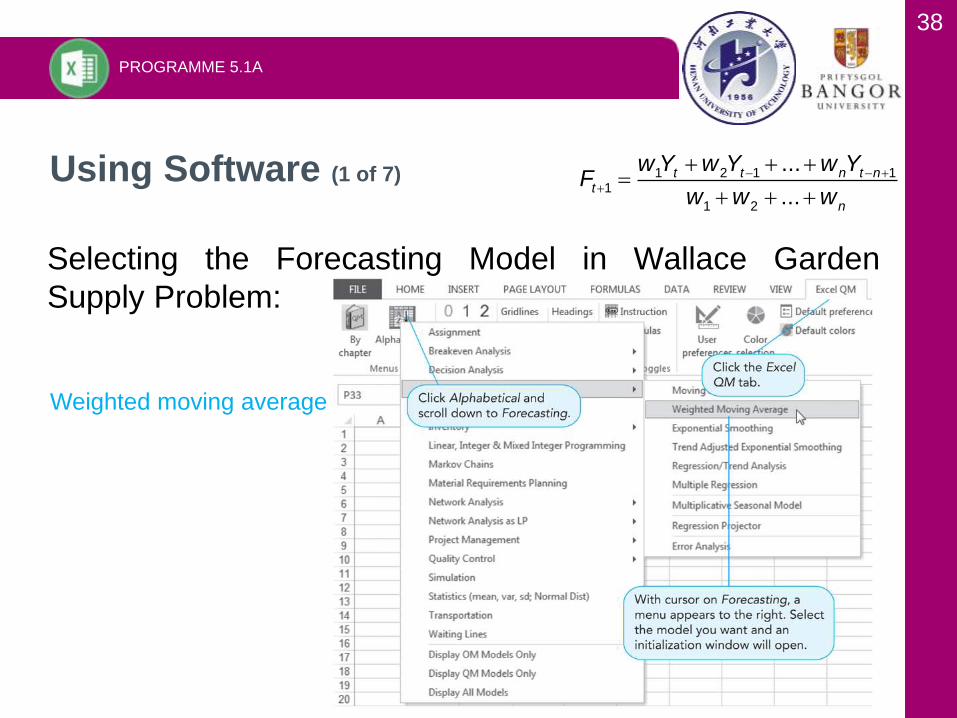
Selecting the Forecasting Model in Wallace Garden
Supply Problem:
Using Software (1 of 7)
PROGRAMME 5.1A
Weighted moving average
1 2 1 11
1 2
...
...t t n t n
t
n
w Y w Y w YF
w w w

39
Weighted Moving Average Forecast for Wallace Garden
Supply:
Wallace Garden Supply (4 of 4)
1 2 1 11
1 2
...
...t t n t n
t
n
w Y w Y w YF
w w w
Weights of 3 for the most recent observation, 2 for the next observation,
and 1 for the most distant observation. The sum of weights is 6!
40
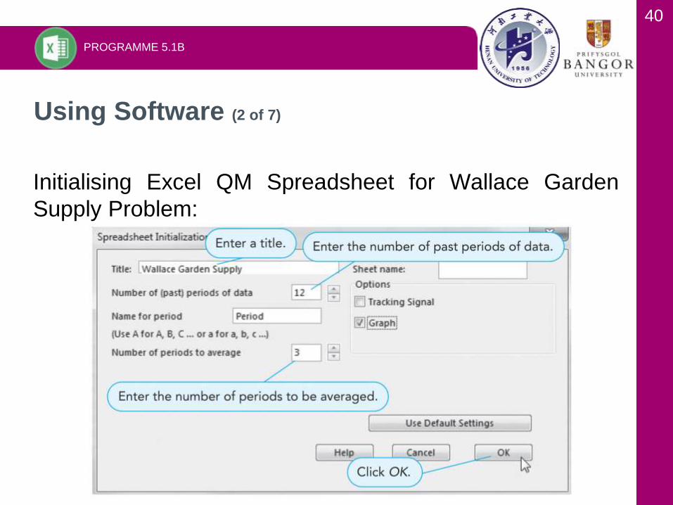
Initialising Excel QM Spreadsheet for Wallace Garden
Supply Problem:
Using Software (2 of 7)
PROGRAMME 5.1B
41
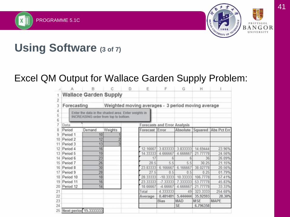
Excel QM Output for Wallace Garden Supply Problem:
Using Software (3 of 7)
PROGRAMME 5.1C
42
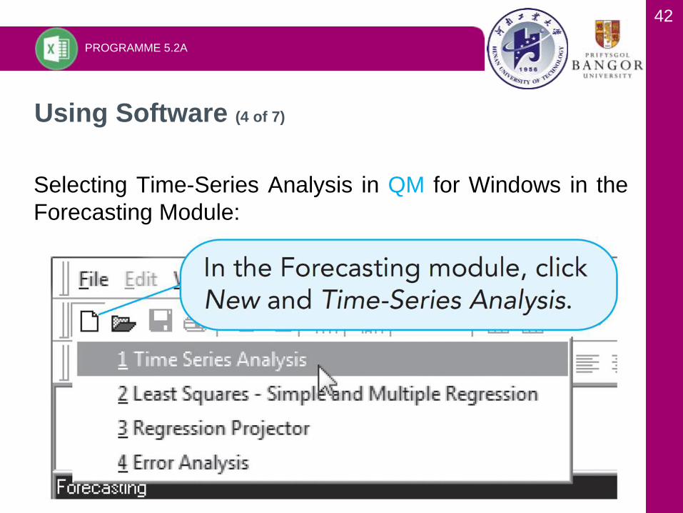
Selecting Time-Series Analysis in QM for Windows in the
Forecasting Module:
Using Software (4 of 7)
PROGRAMME 5.2A

43
Entering Data for Port of Baltimore Example in QM for
Windows:
Using Software (5 of 7)
PROGRAMME 5.2B

44
Selecting the Model and Entering Data for Port of
Baltimore Example in QM for Windows:
Using Software (6 of 7)
PROGRAMME 5.2C

45
Output for Port of Baltimore Example in QM for Windows:
Using Software (7 of 7)
PROGRAMME 5.2D

46
• Exponential smoothing does not respond to trends
If there is a trend present in a time series, the
forecasting model must account for this and cannot
simply average past values!
• A more complex model can be used
• The basic idea is
o Develop an exponential smoothing forecast, and
o Adjust it for the trend!
Forecasting Models – Trend and Random
Variations
Trend (T) is the gradual upward or downward movement
of the data over time.
47
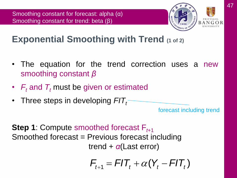
• The equation for the trend correction uses a new
smoothing constant β
• Ft and Tt must be given or estimated
• Three steps in developing FITt
Step 1: Compute smoothed forecast Ft+1
Smoothed forecast = Previous forecast including
trend + α(Last error)
Exponential Smoothing with Trend (1 of 2)
1 ( )t t t tF FIT Y FIT
forecast including trend
Smoothing constant for forecast: alpha (α)
Smoothing constant for trend: beta (β)
48
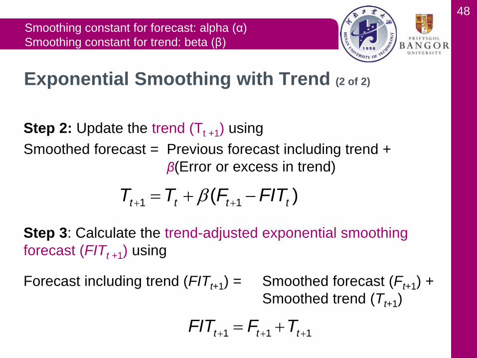
Step 2: Update the trend (Tt +1) using
Smoothed forecast = Previous forecast including trend +
β(Error or excess in trend)
Step 3: Calculate the trend-adjusted exponential smoothing
forecast (FITt +1) using
Forecast including trend (FITt+1) = Smoothed forecast (Ft+1) +
Smoothed trend (Tt+1)
Exponential Smoothing with Trend (2 of 2)
1 1( )t t t tT T F FIT
1 1 1t t tFIT F T
Smoothing constant for forecast: alpha (α)
Smoothing constant for trend: beta (β)
49
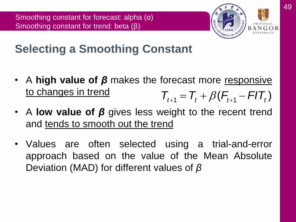
• A high value of β makes the forecast more responsive
to changes in trend
• A low value of β gives less weight to the recent trend
and tends to smooth out the trend
• Values are often selected using a trial-and-error
approach based on the value of the Mean Absolute
Deviation (MAD) for different values of β
Selecting a Smoothing Constant
1 1( )t t t tT T F FIT
Smoothing constant for forecast: alpha (α)
Smoothing constant for trend: beta (β)
50
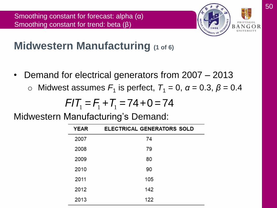
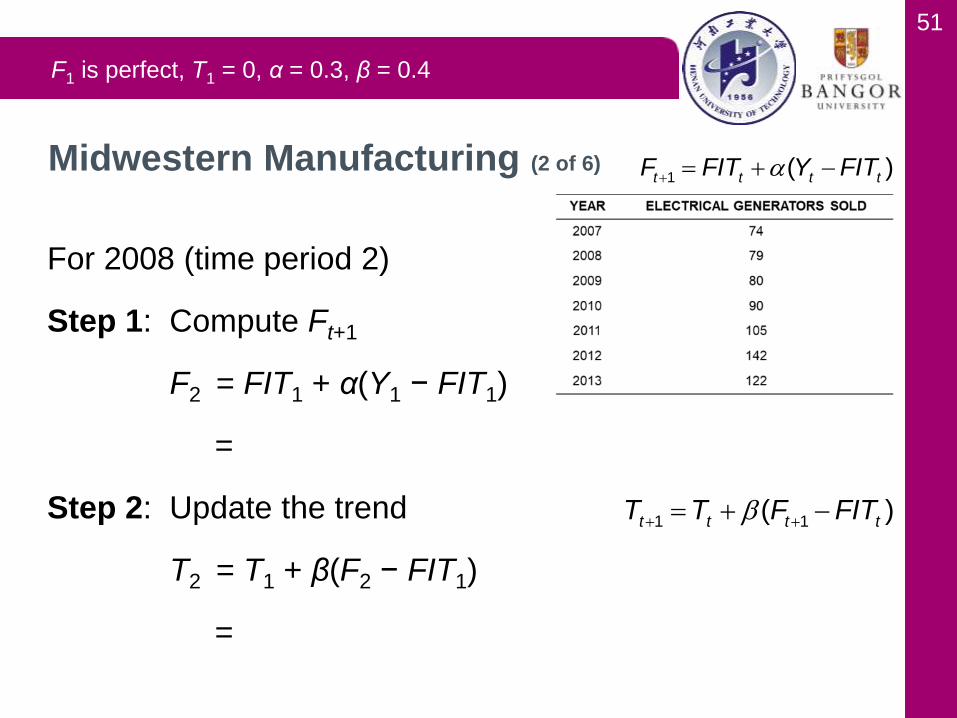
• Demand for electrical generators from 2007 – 2013
o Midwest assumes F1 is perfect, T1 = 0, α = 0.3, β = 0.4
Midwestern Manufacturing’s Demand:
Midwestern Manufacturing (1 of 6)
FIT1 =F1 +T1 = 74+0 = 74
Smoothing constant for forecast: alpha (α)
Smoothing constant for trend: beta (β)
51
For 2008 (time period 2)
Step 1: Compute Ft+1
F2 = FIT1 + α(Y1 − FIT1)
=
Step 2: Update the trend
T2 = T1 + β(F2 − FIT1)
=
Midwestern Manufacturing (2 of 6)
F1 is perfect, T1 = 0, α = 0.3, β = 0.4
1 ( )t t t tF FIT Y FIT
1 1( )t t t tT T F FIT
52
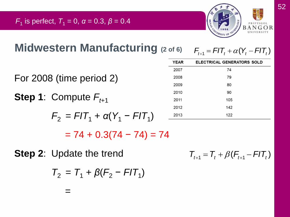
For 2008 (time period 2)
Step 1: Compute Ft+1
F2 = FIT1 + α(Y1 − FIT1)
= 74 + 0.3(74 − 74) = 74
Step 2: Update the trend
T2 = T1 + β(F2 − FIT1)
=
Midwestern Manufacturing (2 of 6)
F1 is perfect, T1 = 0, α = 0.3, β = 0.4
1 ( )t t t tF FIT Y FIT
1 1( )t t t tT T F FIT
53
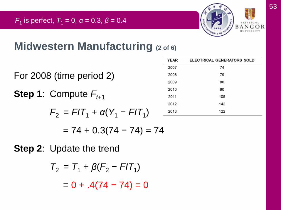
For 2008 (time period 2)
Step 1: Compute Ft+1
F2 = FIT1 + α(Y1 − FIT1)
= 74 + 0.3(74 − 74) = 74
Step 2: Update the trend
T2 = T1 + β(F2 − FIT1)
= 0 + .4(74 − 74) = 0
Midwestern Manufacturing (2 of 6)
F1 is perfect, T1 = 0, α = 0.3, β = 0.4
54
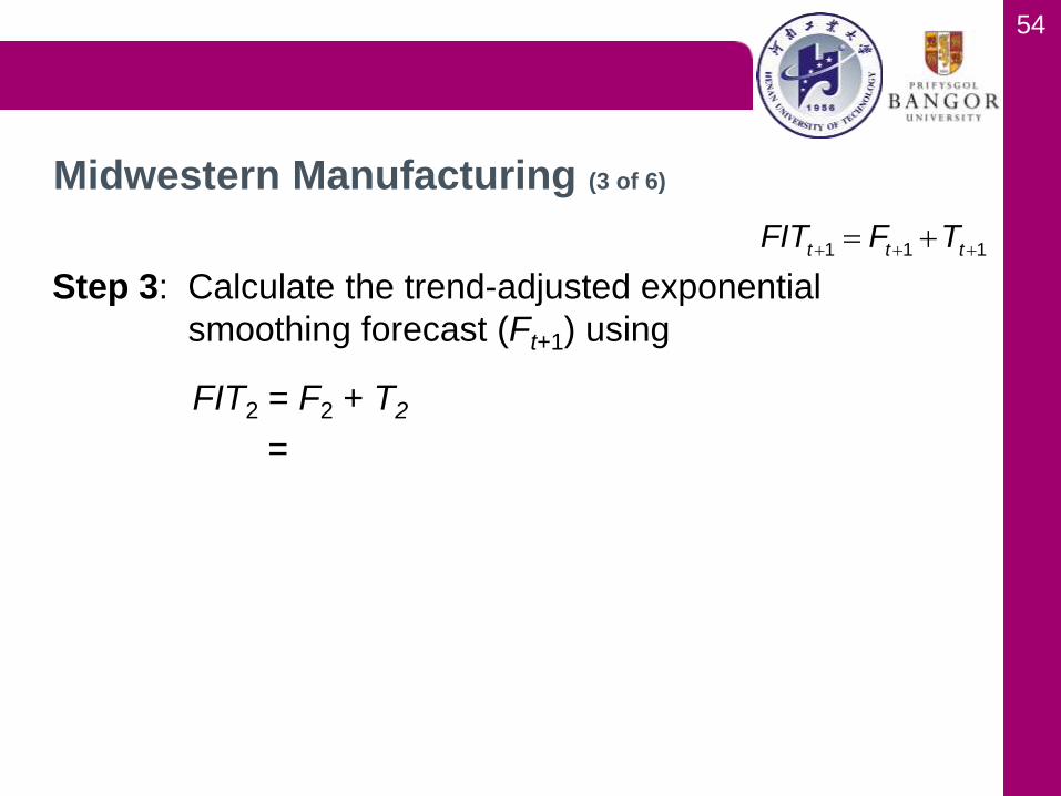
Step 3: Calculate the trend-adjusted exponential
smoothing forecast (Ft+1) using
FIT2 = F2 + T2
=
Midwestern Manufacturing (3 of 6)
1 1 1t t tFIT F T
55
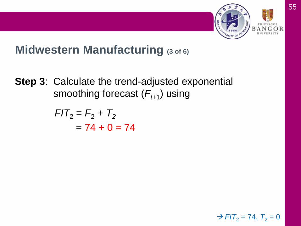
Step 3: Calculate the trend-adjusted exponential
smoothing forecast (Ft+1) using
FIT2 = F2 + T2
= 74 + 0 = 74
Midwestern Manufacturing (3 of 6)
FIT2 = 74, T2 = 0

56
For 2009 (time period 3)
Step 1: F3 = FIT2 + α(Y2 − FIT2)
=
Step 2: T3 = T2 + β(F3 − FIT2)
=
Step 3: FIT3 = F3 + T3
=
Midwestern Manufacturing (4 of 6)
F1 is perfect, T1 = 0, α = 0.3, β = 0.4
FIT2 = 74, T2 = 0
1 ( )t t t tF FIT Y FIT
1 1( )t t t tT T F FIT
1 1 1t t tFIT F T
57
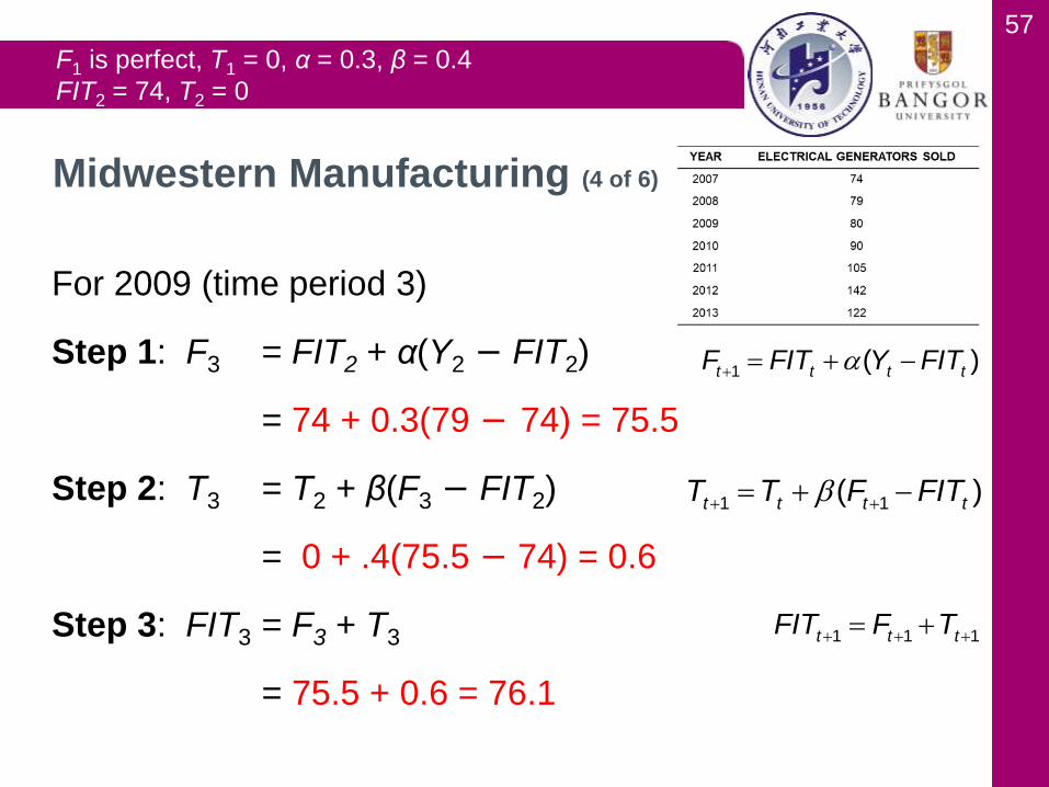
For 2009 (time period 3)
Step 1: F3 = FIT2 + α(Y2 − FIT2)
= 74 + 0.3(79 − 74) = 75.5
Step 2: T3 = T2 + β(F3 − FIT2)
= 0 + .4(75.5 − 74) = 0.6
Step 3: FIT3 = F3 + T3
= 75.5 + 0.6 = 76.1
Midwestern Manufacturing (4 of 6)
F1 is perfect, T1 = 0, α = 0.3, β = 0.4
FIT2 = 74, T2 = 0
1 ( )t t t tF FIT Y FIT
1 1( )t t t tT T F FIT
1 1 1t t tFIT F T

58
Midwestern Manufacturing Exponential Smoothing with
Trend Forecasts:
Midwestern Manufacturing (5 of 6)
59
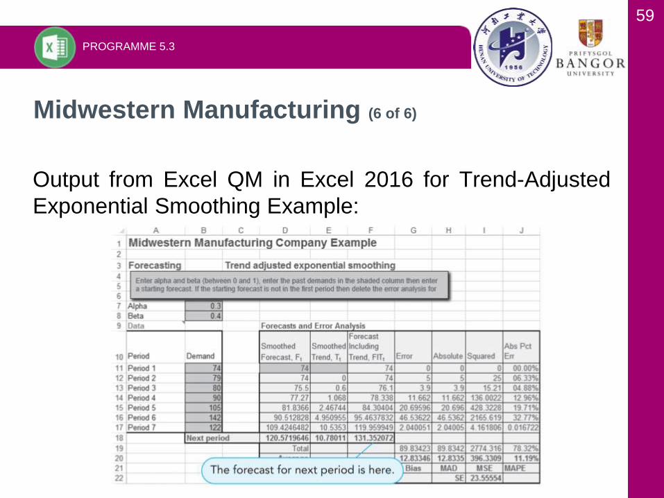
Output from Excel QM in Excel 2016 for Trend-Adjusted
Exponential Smoothing Example:
Midwestern Manufacturing (6 of 6)
PROGRAMME 5.3

60
• Fits a trend line to a series of
historical data points – and
then
• projects the line into the
future for medium- to long-
range forecasts
• Trend equations can be
developed based on
exponential or quadratic models
• Linear model developed
using regression analysis is
simplest
Trend Projections (1 of 2)
0 1Y b b X
A trend line is simply a linear regression
equation in which the independent variable
(X) is the time period.
61
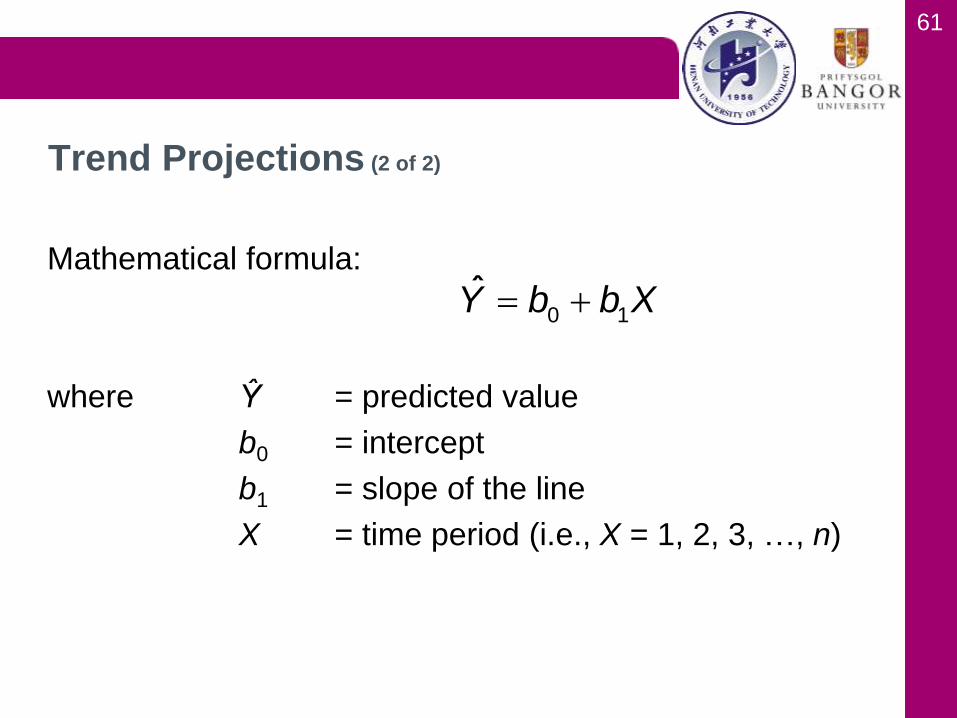
Mathematical formula:
where Ŷ = predicted value
b0 = intercept
b1 = slope of the line
X = time period (i.e., X = 1, 2, 3, …, n)
Trend Projections (2 of 2)
0 1Y b b X

62
• Based on least squares regression, the forecast
equation is
• Year 2014 is coded as X = 8
(sales in 2014)= 56.71 + 10.54(8)
= 141.03, or 141 generators
• For X = 9
(sales in 2015)= 56.71 + 10.54(9)
= 151.57, or 152 generators
Midwestern Manufacturing (1 of 4)
ˆ 56.71 10.54XY
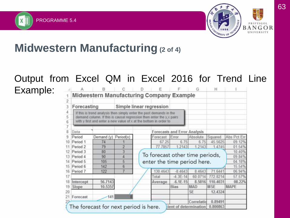
63
Output from Excel QM in Excel 2016 for Trend Line
Example:
Midwestern Manufacturing (2 of 4)
PROGRAMME 5.4
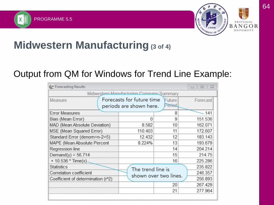
64
Output from QM for Windows for Trend Line Example:
Midwestern Manufacturing (3 of 4)
PROGRAMME 5.5

65
Generator Demand and Projections for Next Three Years
Based on Trend Line:
Midwestern Manufacturing (4 of 4)

66
Example:
• Demand for coal and fuel oil usually peaks during the
cold winter months.
Recurring variations over time may indicate the need
for seasonal adjustments in the trend line
• A seasonal index indicates how a particular season
compares with an average season
o An index of 1 indicates an average season
o An index > 1 indicates the season is higher than average
o An index < 1 indicates a season lower than average
Seasonal Variations
Analysing data in monthly or quarterly terms makes it
easy to spot seasonal patterns!
When no trend is present, the index
can be found by dividing the average
value for a particular season by the
average of all the data

67
• Each observation in the time series is divided by the
appropriate seasonal index to remove the impact of the
seasonality Deseasonalised data is created!
• Once deseasonalised forecasts have been developed,
values are multiplied by the seasonal indices
Seasonal indices are computed in two ways:
o Overall average (when no trend is present)
o Centered-moving-average approach (when trend is
present)
Seasonal Indices
68
• Divide average value for each season by the average of
all data
o Telephone answering machines at Eichler Supplies
o Sales data for the past two years for one model
o Create a forecast that includes seasonality
Seasonal Indices with No Trend (1 of 3)
An index of 1 means the season is average!

69
Answering Machine Sales and Seasonal Indices:
Seasonal Indices with No Trend (2 of 3)
First: The average demand
in each month is computed.
(80 + 100) /2 = = 90 / 94
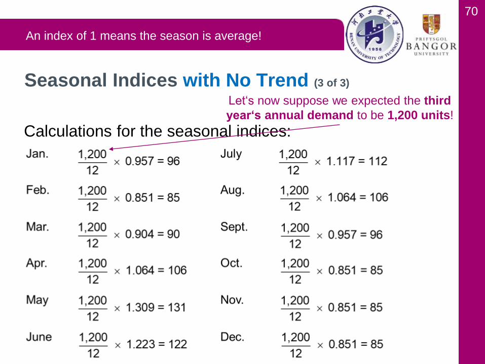
70
Calculations for the seasonal indices:
Seasonal Indices with No Trend (3 of 3)
An index of 1 means the season is average!
Let‘s now suppose we expected the third
year‘s annual demand to be 1,200 units!

71
• When both trend and seasonal components are present
in a time series, a change from one month to the next
could be due to a trend, to a seasonal variation, or
simply to random fluctuations.
• Centered moving average (CMA) approach prevents
trend being interpreted as seasonal
New example:
• Turner Industries sales contain both trend and
seasonal components
Seasonal Indices with Trend (1 of 2)
72
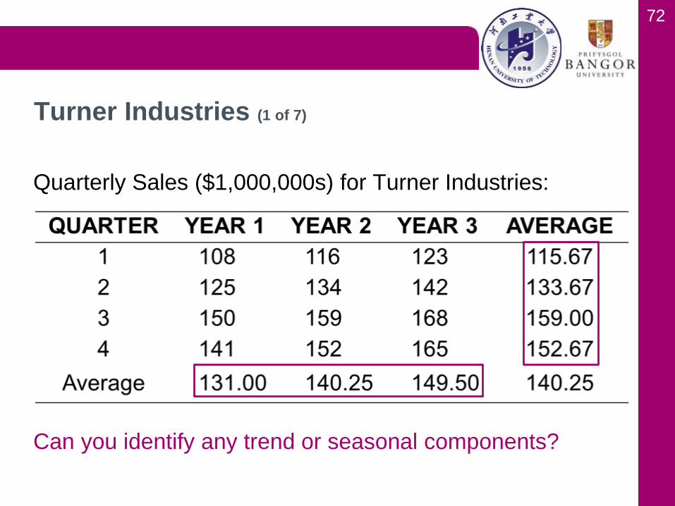
Quarterly Sales ($1,000,000s) for Turner Industries:
Can you identify any trend or seasonal components?
Turner Industries (1 of 7)

73
Steps in Centered moving average (CMA):
1. Compute the CMA for each observation (where
possible) … e.g. quarter 3 of year 1
2. Compute the seasonal ratio = Observation÷CMA for
that observation
3. Average seasonal ratios to get seasonal indices
4. If seasonal indices do not add to the number of
seasons, multiply each index by (Number of
seasons)÷(Sum of indices)
Seasonal Indices with Trend (2 of 2)

74
Quarterly Sales ($1,000,000s) for Turner Industries:
Turner Industries (2 of 7)
Contains trend and seasonal components!
75
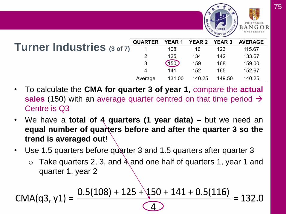
• To calculate the CMA for quarter 3 of year 1, compare the actual
sales (150) with an average quarter centred on that time period
Centre is Q3
• We have a total of 4 quarters (1 year data) – but we need an
equal number of quarters before and after the quarter 3 so the
trend is averaged out!
• Use 1.5 quarters before quarter 3 and 1.5 quarters after quarter 3
o Take quarters 2, 3, and 4 and one half of quarters 1, year 1 and
quarter 1, year 2
Turner Industries (3 of 7)
CMA(q3,y1)=0.5(108)+125+150+141+0.5(116)
4=132.0
76
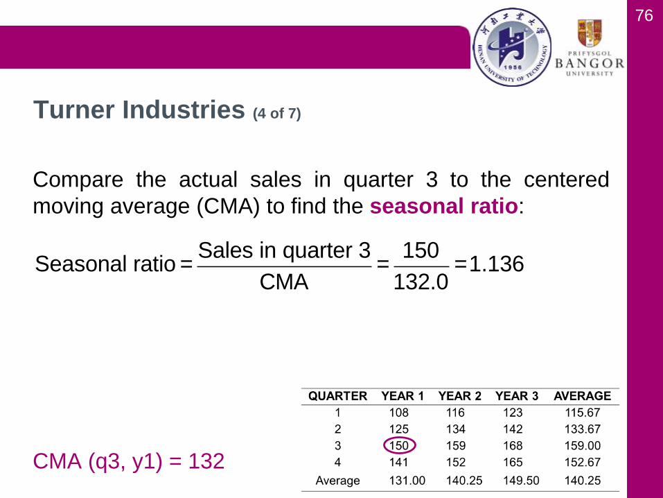
Compare the actual sales in quarter 3 to the centered
moving average (CMA) to find the seasonal ratio:
CMA (q3, y1) = 132
Turner Industries (4 of 7)
Seasonal ratio =Sales in quarter 3
CMA=
150
132.0=1.136
77
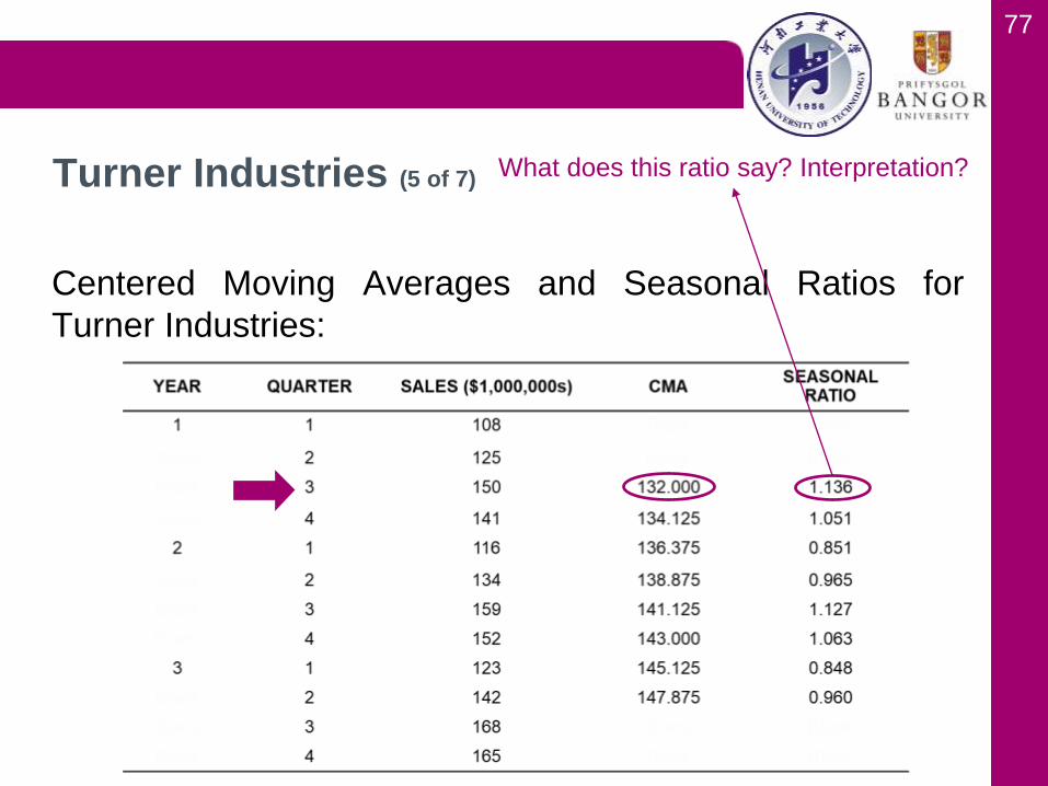
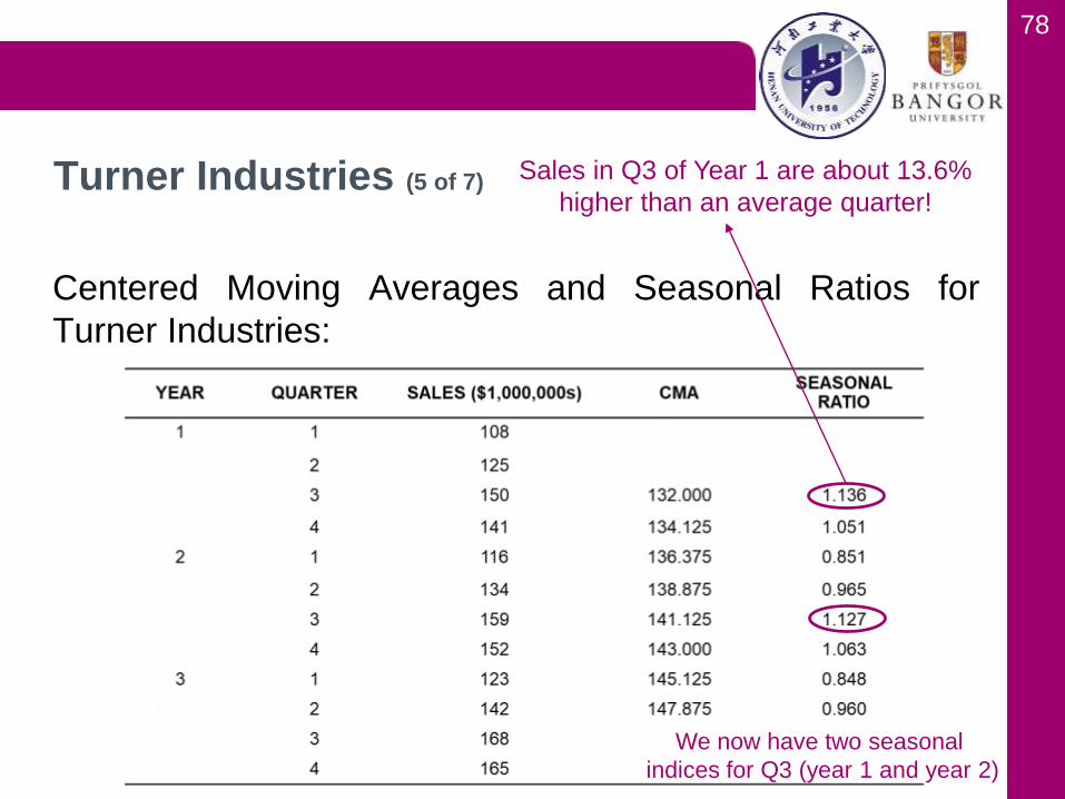
Centered Moving Averages and Seasonal Ratios for
Turner Industries:
Turner Industries (5 of 7) What does this ratio say? Interpretation?
78
Centered Moving Averages and Seasonal Ratios for
Turner Industries:
Turner Industries (5 of 7)
We now have two seasonal
indices for Q3 (year 1 and year 2)
Sales in Q3 of Year 1 are about 13.6%
higher than an average quarter!

79
The two seasonal ratios for each quarter are averaged
to get the seasonal index:
Index for quarter 1 = I1 = (0.851 + 0.848)÷2 = 0.85
Index for quarter 2 = I2 = (0.965 + 0.960)÷2 = 0.96
Index for quarter 3 = I3 = (1.136 + 1.127)÷2 = 1.13
Index for quarter 4 = I4 = (1.051 + 1.063)÷2 = 1.06
The sum of these indices should be the number of
seasons (4) since an average season should have
an index of 1.
Turner Industries (6 of 7)
If the sum were not 4, an adjustment would be made. We would
multiply each index by 4 and divide this by the sum of the indices.
80
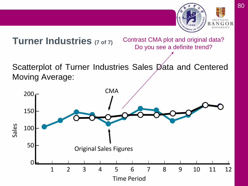
Scatterplot of Turner Industries Sales Data and Centered
Moving Average:
Turner Industries (7 of 7) Contrast CMA plot and original data?
Do you see a definite trend?
81
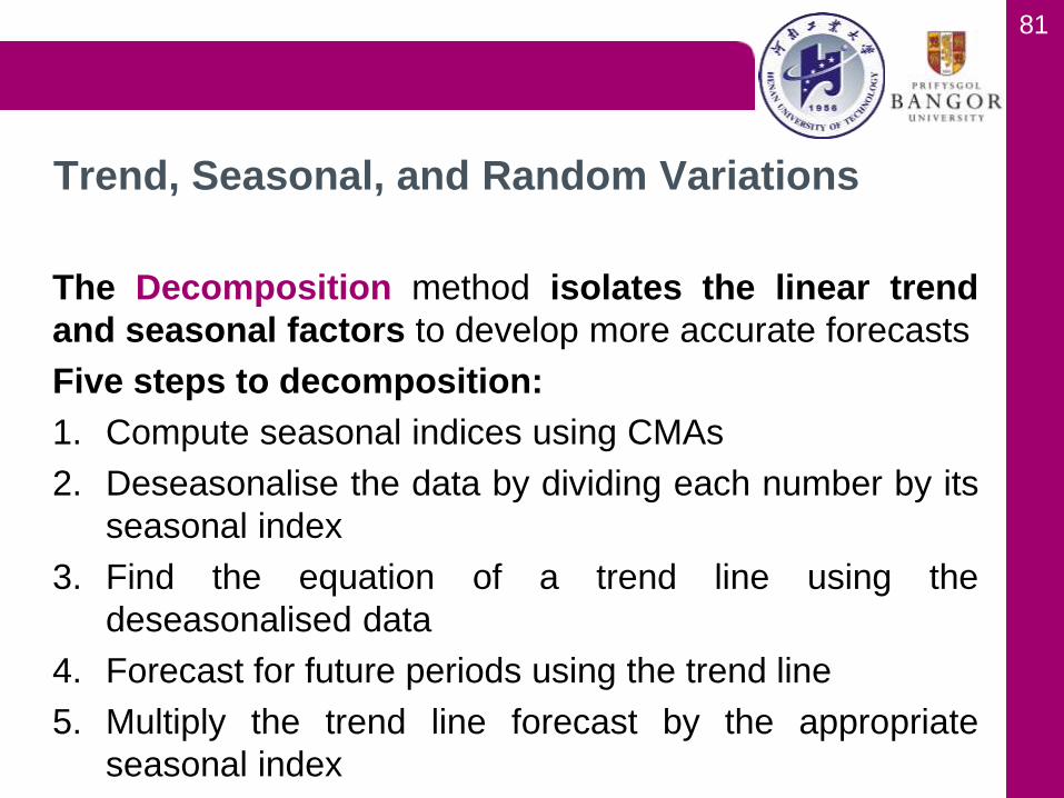
The Decomposition method isolates the linear trend
and seasonal factors to develop more accurate forecasts
Five steps to decomposition:
1. Compute seasonal indices using CMAs
2. Deseasonalise the data by dividing each number by its
seasonal index
3. Find the equation of a trend line using the
deseasonalised data
4. Forecast for future periods using the trend line
5. Multiply the trend line forecast by the appropriate
seasonal index
Trend, Seasonal, and Random Variations

82
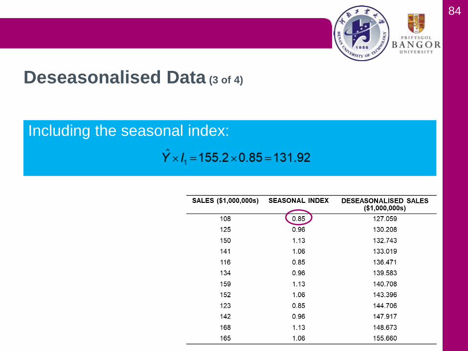
Deseasonalised Data for Turner Industries (1 of 4)
Steps 1 and 2:
= 108 / 0.85
Compute seasonal indices using CMAs
Deseasonalise the data by dividing each number by its seasonal index
83
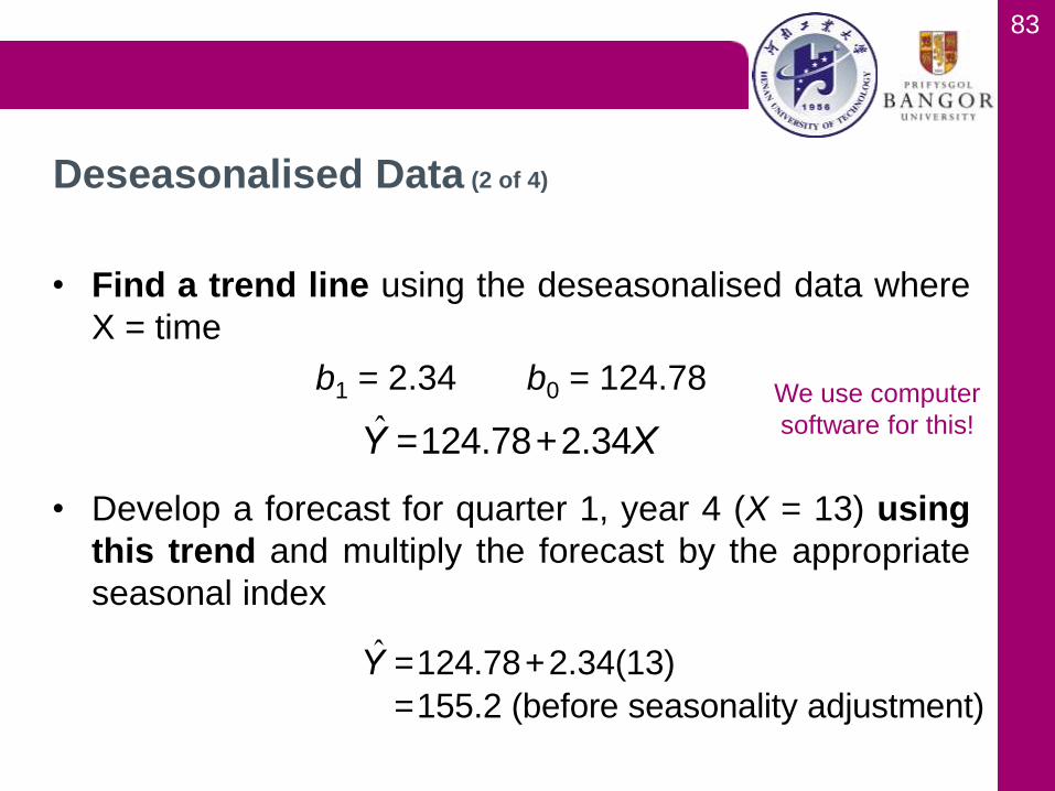
• Find a trend line using the deseasonalised data where
X = time
b1 = 2.34 b0 = 124.78
• Develop a forecast for quarter 1, year 4 (X = 13) using
this trend and multiply the forecast by the appropriate
seasonal index
Deseasonalised Data (2 of 4)
Y =124.78+2.34X
Y =124.78+ 2.34(13)
=155.2 (before seasonality adjustment)
We use computer
software for this!
84
Deseasonalised Data (3 of 4)
Including the seasonal index:
85
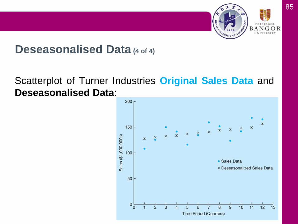
Scatterplot of Turner Industries Original Sales Data and
Deseasonalised Data:
Deseasonalised Data (4 of 4)
86
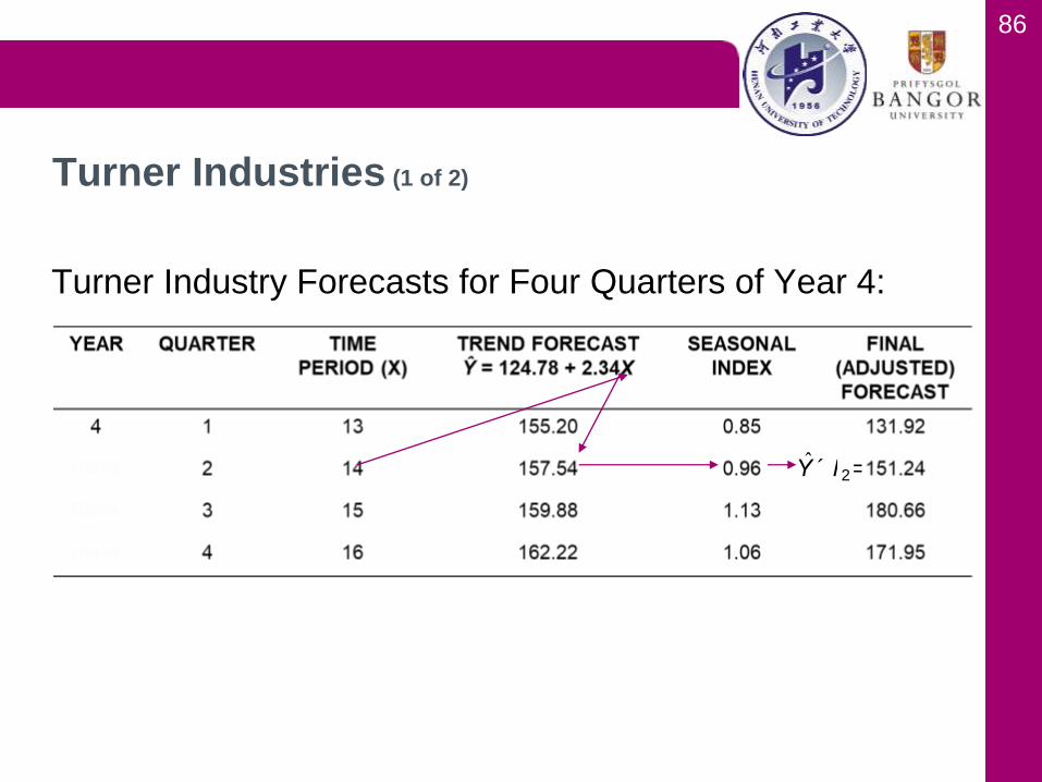
Turner Industry Forecasts for Four Quarters of Year 4:
Turner Industries (1 of 2)
Y ´ I1 =155.2´0.85 =131.922
87
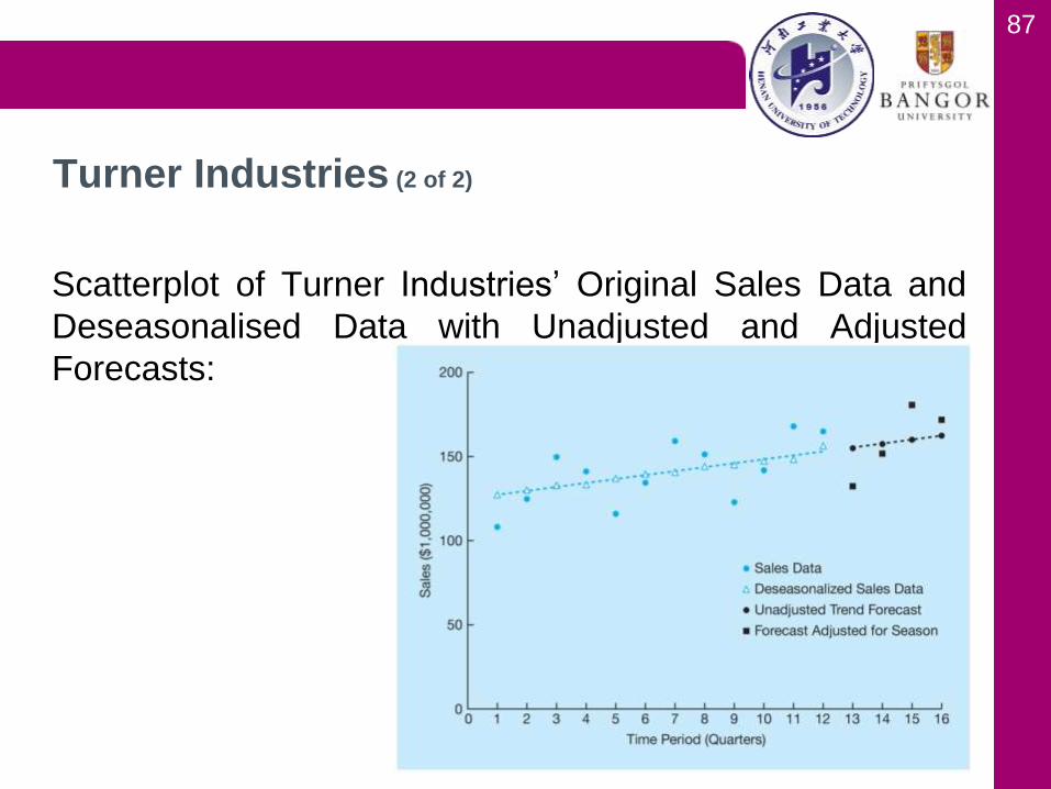
Scatterplot of Turner Industries’ Original Sales Data and
Deseasonalised Data with Unadjusted and Adjusted
Forecasts:
Turner Industries (2 of 2)

90
• Multiple regression can be used to forecast both trend
and seasonal components
o One independent variable is time
o Dummy independent variables are used to represent the
seasons
o An additive decomposition model
where X1 = time period
X2 = 1 if quarter 2, 0 otherwise
X3 = 1 if quarter 3, 0 otherwise
X4 = 1 if quarter 4, 0 otherwise
Using Regression with Trend and Seasonal (1 of 5)
Y = a+b1X1 +b2X2 +b3X3 +b4X4
95
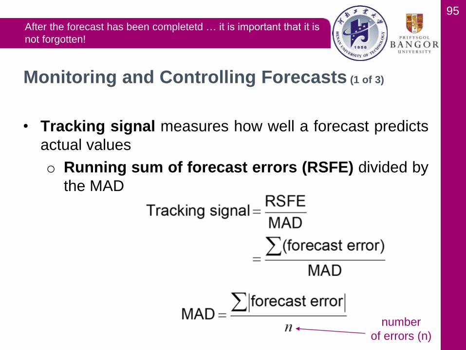
• Tracking signal measures how well a forecast predicts
actual values
o Running sum of forecast errors (RSFE) divided by
the MAD
Monitoring and Controlling Forecasts (1 of 3)
After the forecast has been completetd … it is important that it is
not forgotten!
number
of errors (n)
96
• Positive tracking signals indicate demand is greater
than forecast
• Negative tracking signals indicate demand is less
than forecast
• A good forecast will have about as much positive error
as negative error
• Problems are indicated when the signal trips either the
upper or lower predetermined limits
Choose reasonable values for these limits!
Monitoring and Controlling Forecasts (2 of 3)
97
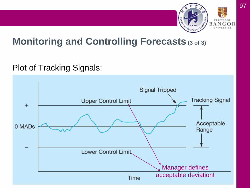
Plot of Tracking Signals:
Monitoring and Controlling Forecasts (3 of 3)
Manager defines
acceptable deviation!
98
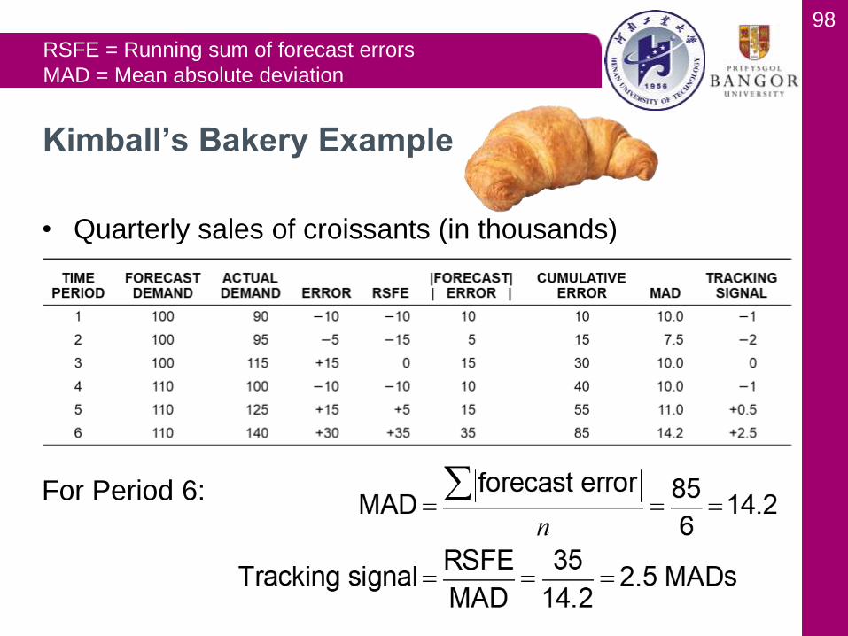
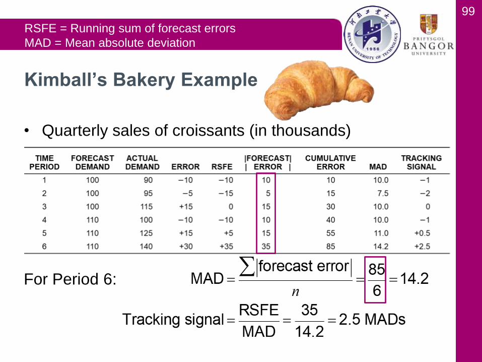
• Quarterly sales of croissants (in thousands)
For Period 6:
Kimball’s Bakery Example
RSFE = Running sum of forecast errors
MAD = Mean absolute deviation
99
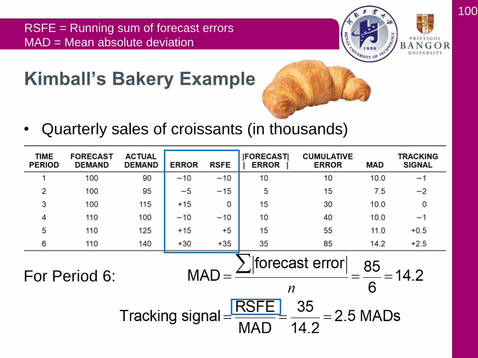
• Quarterly sales of croissants (in thousands)
For Period 6:
Kimball’s Bakery Example
RSFE = Running sum of forecast errors
MAD = Mean absolute deviation
100
• Quarterly sales of croissants (in thousands)
For Period 6:
Kimball’s Bakery Example
RSFE = Running sum of forecast errors
MAD = Mean absolute deviation
101
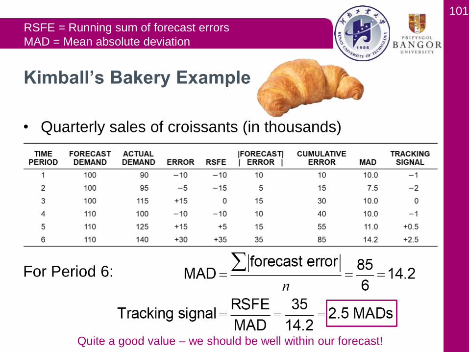
• Quarterly sales of croissants (in thousands)
For Period 6:
Kimball’s Bakery Example
RSFE = Running sum of forecast errors
MAD = Mean absolute deviation
Quite a good value – we should be well within our forecast!

102
• Computer monitoring of tracking signals and self-
adjustment if a limit is tripped
• In exponential smoothing, the values of α and β are
adjusted when the computer detects an excessive
amount of variation!
Adaptive Smoothing

103
• End of chapter self-test 1-14
(pp. 243-244)
Compile all answers into one
document and submit at the
beginning of the next lecture!
On the top of the document,
write your Pinyin-Name and
Student ID.
• Please read Chapter 6!
Homework --- Chapter 5
Related Documents