5.1 Chapter 5: Equilibrium of a Rigid Body Chapter Objectives • To develop the equations of equilibrium for a rigid body. • To introduce the concept of a free-body diagram for a rigid body. • To show how to solve rigid body equilibrium problems using the equations of equilibrium. In this chapter, we will describe the various types of supports that are used with rigid body equilibrium problems. • We will then show how free-body diagrams and equilibrium equations are used to determine unknown forces and couples acting on a rigid body. 5.1 Conditions for Rigid-Body Equilibrium When the force and couple are both equal to zero, the external forces form a system equivalent to zero and the rigid body is said to be in equilibrium. • Hence two equations of equilibrium for a rigid body can be summarized as follows. ∑F = 0 Necessary and sufficient conditions for ∑M = 0 the equilibrium of a rigid body. • We may express the necessary and sufficient conditions for the equilibrium of a rigid body in the following scalar form. ∑Fx = 0 ∑Fy = 0 ∑Fz = 0 ∑Mx = 0 ∑My = 0 ∑Mz = 0 Equilibrium in Two Dimensions First, we will consider the case in which the force system acting on a rigid body is in a single plane. • This type of force system is referred to as a two-dimensional or coplanar force system. • Forces acting on the body are in the same plane. • Couple moments acting on the body are perpendicular to this plane. 5.2 Free-Body Diagrams The best way to account for all of the known and unknown external forces acting on a rigid body is to draw the free-body diagram.

Welcome message from author
This document is posted to help you gain knowledge. Please leave a comment to let me know what you think about it! Share it to your friends and learn new things together.
Transcript

5.1
Chapter 5: Equilibrium of a Rigid Body
Chapter Objectives
• To develop the equations of equilibrium for a rigid body.
• To introduce the concept of a free-body diagram for a rigid body.
• To show how to solve rigid body equilibrium problems using the equations of
equilibrium.
In this chapter, we will describe the various types of supports that are used with rigid
body equilibrium problems.
• We will then show how free-body diagrams and equilibrium equations are used to
determine unknown forces and couples acting on a rigid body.
5.1 Conditions for Rigid-Body Equilibrium
When the force and couple are both equal to zero, the external forces form a
system equivalent to zero and the rigid body is said to be in equilibrium.
• Hence two equations of equilibrium for a rigid body can be summarized as
follows.
∑F = 0 Necessary and sufficient conditions for
∑M = 0 the equilibrium of a rigid body.
• We may express the necessary and sufficient conditions for the equilibrium of
a rigid body in the following scalar form.
∑Fx = 0 ∑Fy = 0 ∑Fz = 0
∑Mx = 0 ∑My = 0 ∑Mz = 0
Equilibrium in Two Dimensions
First, we will consider the case in which the force system acting on a rigid body is in a
single plane.
• This type of force system is referred to as a two-dimensional or coplanar force
system.
• Forces acting on the body are in the same plane.
• Couple moments acting on the body are perpendicular to this plane.
5.2 Free-Body Diagrams
The best way to account for all of the known and unknown external forces acting
on a rigid body is to draw the free-body diagram.

5.2
Support Reactions
“Reactions” are the forces through which the ground and other bodies oppose a
possible motion of the free body.
• Reactions are exerted at points where the free body is supported or connected
to other bodies.
It is important to understand how to replace certain supports with the appropriate
constraining forces.
• In general, if a support prevents translation, then a force is developed on the
body in that direction.
• Likewise, if rotation is prevented, a couple moment is exerted on the rigid body.
Reactions exerted on two-dimensional structure may be divided into three groups,
corresponding to three types of supports or connections.
1. Reaction equivalent to a force with a known line of action (1 unknown).
• This reaction prevents translation of the free body in one direction, but it
cannot prevent the body from rotating about the connection.
• For each of these supports there is only one unknown involved, that is, the
magnitude of the reaction.
• The line of action is known.
The most common examples are as follows.
a. Roller support
A roller support prevents vertical translation.
b. Link
A link prevents translation along the axis of the link.

5.3
c. Cables (weightless)
2. Reaction equivalent to a force with an unknown line of action (2 unknowns).
• This reaction prevents translation of the free body in all directions, but it
cannot prevent the body from rotating about the connection.
• The magnitude and direction of the reactive force is unknown.
• Normally we work with the components, thus fixing the directions but not
knowing the magnitude of the components.
The most common examples are as follows.
a. Pin
A pin prevents vertical and horizontal translation.
b. Ball and socket joint (2-D)
A ball and socket joint prevents vertical and horizontal translation.
3. Reaction equivalent to a force and a couple (3 unknowns).
• This reaction is caused by “fixed supports” which oppose any motion of the
free body and thus constrain it completely, preventing both translation and
rotation.
• Reactions of this group involve three unknowns, consisting usually of the two
components of the force and the moment of the couple.

5.4
The most common example is as follows.
a. Fixed end
The fixed end prevents vertical and horizontal translation, and prevents
rotation.
When the sense of an unknown force or couple is not clearly apparent, no attempt
should be made to determine the correct direction.
• Instead, the sense of the force or couple should be arbitrarily assumed.
• The sign of the answer obtained will indicate whether the assumption is correct
or not.
Internal Forces
If a free-body diagram for the rigid body is drawn, only external forces are shown.
• Internal forces within the rigid body are not represented on a free-body
diagram.
• Internal forces cancel each other, and as a result, do not create an external
effect on the rigid body
Weight and the Center of Gravity
When the weight of a body must be considered, a force resultant representing the
weight is used with its point of application acting through the center of gravity.
Idealized Models
In order to perform a correct force analysis of any object, it is important to
consider a corresponding analytical or idealized model that gives results that
approximate as closely as possible the actual situation.
• Example, consider the underground pump station: Is reinforced concrete slab
acting as simply supported, or fixed-fixed to concrete block walls?
5.5
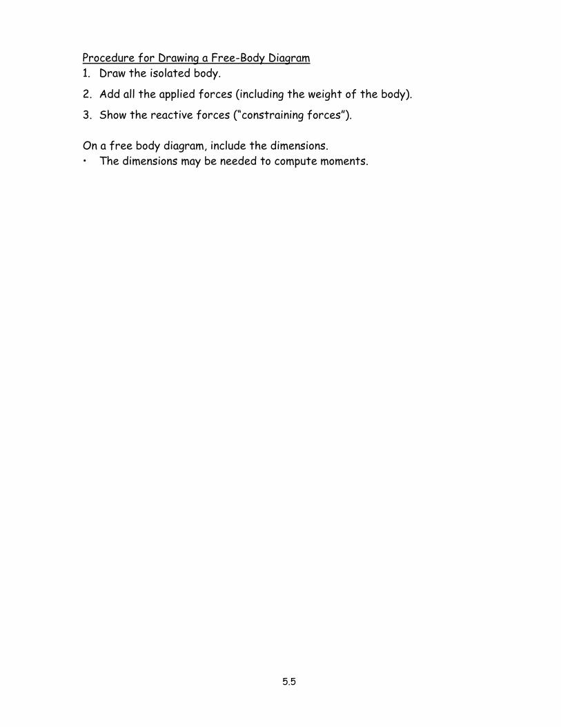
Procedure for Drawing a Free-Body Diagram
1. Draw the isolated body.
2. Add all the applied forces (including the weight of the body).
3. Show the reactive forces (“constraining forces”).
On a free body diagram, include the dimensions.
• The dimensions may be needed to compute moments.

5.6
Example – Free Body Diagram
Given: The loaded W18 x 40 beam shown.
Find: Draw the free body diagram and
solve for the reactions.
Draw the free body diagram.
Steps:
1. Draw the isolated body.
2. Add the applied forces.
3. Show the reactive forces.
a. Does the support at A prevent . . .
1) Horizontal translation?
2) Vertical translation?
3) Rotation?
b. Does the support at B prevent . . .
1) Horizontal translation?
2) Vertical translation?
3) Rotation?
Solve for the reactions.
∑Fx = 0 = (4/5) 75 + Ax
Ax = - 60 kips Ax = 60 kips ←
∑MA = 0 = 10 By – (3/5) 75 (4)
10 By = 180
By = + 18.0 kips By = 18.0 kips ↑
∑MB = 0 = - 10 Ay + (3/5) 75 (6)
10 Ay = 270
Ay = + 27.0 kips Ay = 27.0 kips ↑

5.7
5.3 Equations of Equilibrium
The conditions of equilibrium in two dimensions are as follows.
∑Fx = 0 ∑Fy = 0 ∑Mz = 0
These three equations (called the “equations of statics”) allow solution for no more
than three unknowns.
Alternative Sets of Equilibrium Equations
These three equations may be replaced with another set of equations.
• An alternate set of equilibrium equations may be as follows.
∑Fx = 0 ∑MA = 0 ∑MB = 0
or ∑MA = 0 ∑MB = 0 ∑MC = 0

5.8
Example
Given: Beam loaded as shown.
Find: Range of values for P for a
safe beam:
RA and RB ≤ 25 kips
(i.e. compression in the
columns at A and B)
∑Fx = 0 = Ax Ax = 0 kips
Let RA = 0 kips: ∑MB = 0 = 6 P - 6 (2) – 6 (4) P = 6.0 kips
Check RB ∑Fy = 0 = - 6 – 6 – 6 + RB
RB = 18.0 kips < 25.0 kips OK
Let RA = 25 kips: ∑MB = 0 = - 25 (9) + 6 P - 6 (2) – 6 (4)
6 P = 225 + 12 + 24 = 261 P = 43.5 kips
Check RB ∑Fy = 0 = 25 - 43.5 – 6 – 6 + RB
RB = 30.5 kips > 25.0 kips NG
Let RB = 25 kips: ∑MA = 0 = - 3 P + 9 (25) – 6 (11) – 6 (13)
3 P = 225 – 66 – 78 = 81 P = 27.0 kips
Check RA ∑Fy = 0 = - 27 + 25 – 6 – 6 + RA
RA = 14.0 kips < 25.0 kips OK
Therefore, 6.0 kips ≤ P ≤ 27.0 kips Answer

5.9
5.4 Two- and Three-Force Members
The solution to some equilibrium problems can be simplified if one is able to
recognize members that are subjected to only two or three forces.
Two-Force Members
If a two-force body is in equilibrium, the two forces must have the same
magnitude, same line of action, and opposite sense.
For the corner plate to be in equilibrium the following equilibrium equations must
be satisfied.
∑MA = 0 = F2r d : either F2r = 0 or d = 0, and
∑MB = 0 = F1r d : either F1r = 0 or d = 0
F1r and F2r must be zero; d = 0 is too restrictive (the rigid body would revert to
a particle).
Characteristics of a two-force member:
1. Coplanar or non-coplanar (any shape).
2. Two forces – same magnitude, same line of
action, opposite direction.
3. Direction of two forces is collinear with line of
action connecting points of application.
4. Points need not be at the end of the member.
5. No couple allowed on member.
A truss member is an example of a two-force member.

5.10
Three-Force Members
If a three-force body is in equilibrium, the lines of action of the three forces must
be either concurrent or parallel.
For the rigid body to be in equilibrium the following equilibrium equation must be
satisfied.
∑MA = 0 = + F3 d: either F3 = 0 or d = 0
F3 ≠ 0 (otherwise the system would revert to a two-force system).
Thus d = 0.
For the rigid body to be in equilibrium, the three forces must be either concurrent
(i.e. d = 0), or parallel.
Concurrent forces Parallel forces
5.11
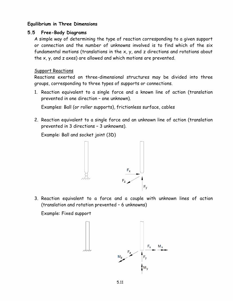
Equilibrium in Three Dimensions
5.5 Free-Body Diagrams
A simple way of determining the type of reaction corresponding to a given support
or connection and the number of unknowns involved is to find which of the six
fundamental motions (translations in the x, y, and z directions and rotations about
the x, y, and z axes) are allowed and which motions are prevented.
Support Reactions
Reactions exerted on three-dimensional structures may be divided into three
groups, corresponding to three types of supports or connections.
1. Reaction equivalent to a single force and a known line of action (translation
prevented in one direction – one unknown).
Examples: Ball (or roller supports), frictionless surface, cables
2. Reaction equivalent to a single force and an unknown line of action (translation
prevented in 3 directions – 3 unknowns).
Example: Ball and socket joint (3D)
3. Reaction equivalent to a force and a couple with unknown lines of action
(translation and rotation prevented – 6 unknowns)
Example: Fixed support

5.12
5.6 Equations of Equilibrium
Vector Equations of Equilibrium
The two conditions of equilibrium of a rigid body are as follows.
∑F = 0 Necessary and sufficient conditions for
∑M = 0 the equilibrium of a rigid body.
Scalar Equations of Equilibrium
Six scalar equations are required to express the conditions for the equilibrium of a
rigid body in the general three-dimensional case.
∑Fx = 0 ∑Fy = 0 ∑Fz = 0
∑Mx = 0 ∑My = 0 ∑Mz = 0
These equations may be solved for no more than six unknowns.
5.7 Constraints and Statical Determinacy
A problem is said to be “statically determinate” when a rigid body is completely
constrained by its supports and the reactions can be determined using the
equations of statics.
Two-Dimensional Analysis
In a two-dimensional analysis, only three independent equilibrium equations are
available.
• When there are more than three unknown reactions, not all of the unknown
reactions can be determined using the equations of equilibrium.
- This type of problem is said to be “statically indeterminate.”
Three-Dimensional Analysis
In a three-dimensional analysis, only six independent equilibrium equations are
available.
• When there are more than six unknown reactions, not all of the unknown
reactions can be determined using the equations of equilibrium.
- This type of problem is said to be “statically indeterminate.”
Redundant Constraints
Determinate

5.13
Determinate
Determinate
Statically indeterminate (with degree of redundancy)
SI1
SI3
SI1
Mobile structure (improperly constrained)
Improper Constraints
“Partially constrained” – The supports provided are not enough to keep the body
(structure) from moving.
• There are fewer unknowns than equations and one of the equilibrium equations
will not be satisfied.
5.14
• If the reactions involve less than three unknowns (2-D) or less than six
unknowns (3-D), there are more equations than there are unknowns, and some of
the equations of equilibrium cannot be satisfied under a general loading
condition.
• The rigid body is said to be only “partially constrained” and should be avoided
since an unstable condition may result.
“Improperly constrained” – There is a sufficient number of constraints, but these
constraints are not properly arranged and the body (structure) is free to move.
• A rigid body is improperly constrained when the supports, even though they
provide a sufficient number of reactions, are arranged in such a way that at
least one of the equilibrium equations is not satisfied.
- Even with three or more unknowns (2-D), or six or more unknowns (3-D), it is
possible that some of the equations of equilibrium will not be satisfied.
- This may occur when the supports are such that the reactions are forces
that are parallel.
• The rigid body is said to be “improperly constrained” and should be avoided
since an unstable condition may result.
Related Documents