Chapter 4 The Laplace Transform in Circuit Analysis

1

The Laplace

Transform in Circuit Analysis

Circuit Elements in the s Domain

The Transfer Function and Natural Response

The Transfer Function and the Convolution Integral

The Transfer Function and the Steady-

State Sinusoidal Response

The Impulse Function in Circuit Analysis

4.14.2-3 Circuit Analysis in the s Domain4.4-54.6

4.7

4.8

Chapter 4

2

Key points

How to represent the initial energy of L, C in the s-domain?

Why the functional forms of natural and steady- state responses are determined by the poles of transfer function H(s) and excitation source X(s), respectively?

Why the output of an LTI circuit is the convolution of the input and impulse response? How to interpret the memory of a circuit by convolution?

3

Circuit Elements in the s Domain

1. Equivalent elements of R, L, C

Section 4.1

4

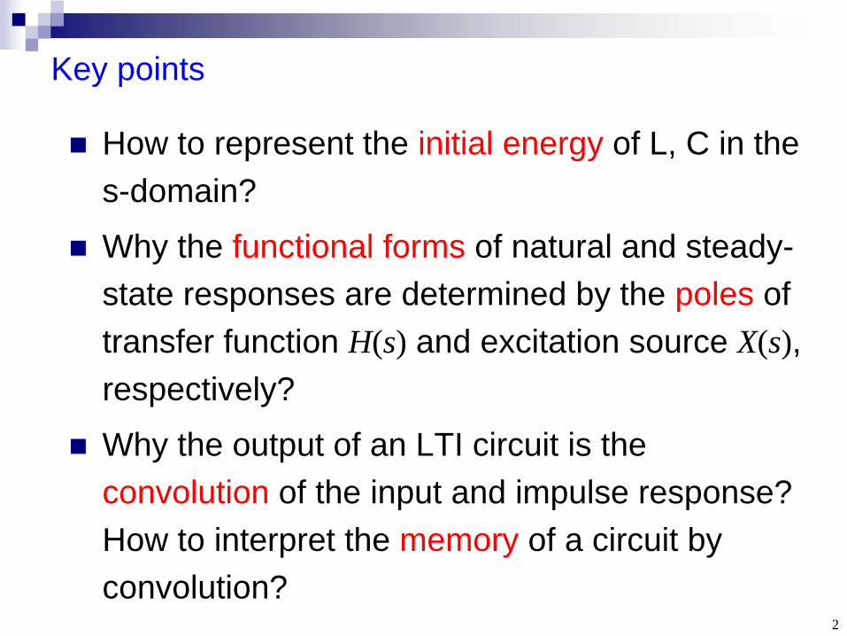
A resistor in the s domain

iv-relation in the time domain:

).()( tiRtv

By operational Laplace transform:

).()(

,)()()(sIRsV

tiLRtiRLtvL

Physical units: V(s) in volt-seconds, I(s) in ampere-seconds.

5

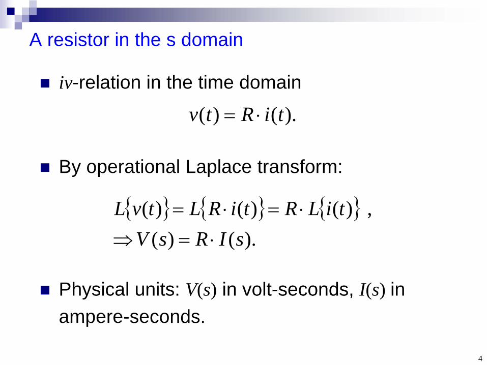
An inductor in the s domain

).()( tidtdLtv

.)()()(

,)()()(

00 LIsIsLIssILsVtiLLtiLLtvL

initial current



6

Equivalent circuit of an inductor

Series equivalent:

Parallel equivalent:

Thévenin Norton

7

A capacitor in the s domain

).()( tvdtdCti

.)()()(

,)()()(

00 CVsVsCVssVCsItvLCtvCLtiL

initial voltage



8

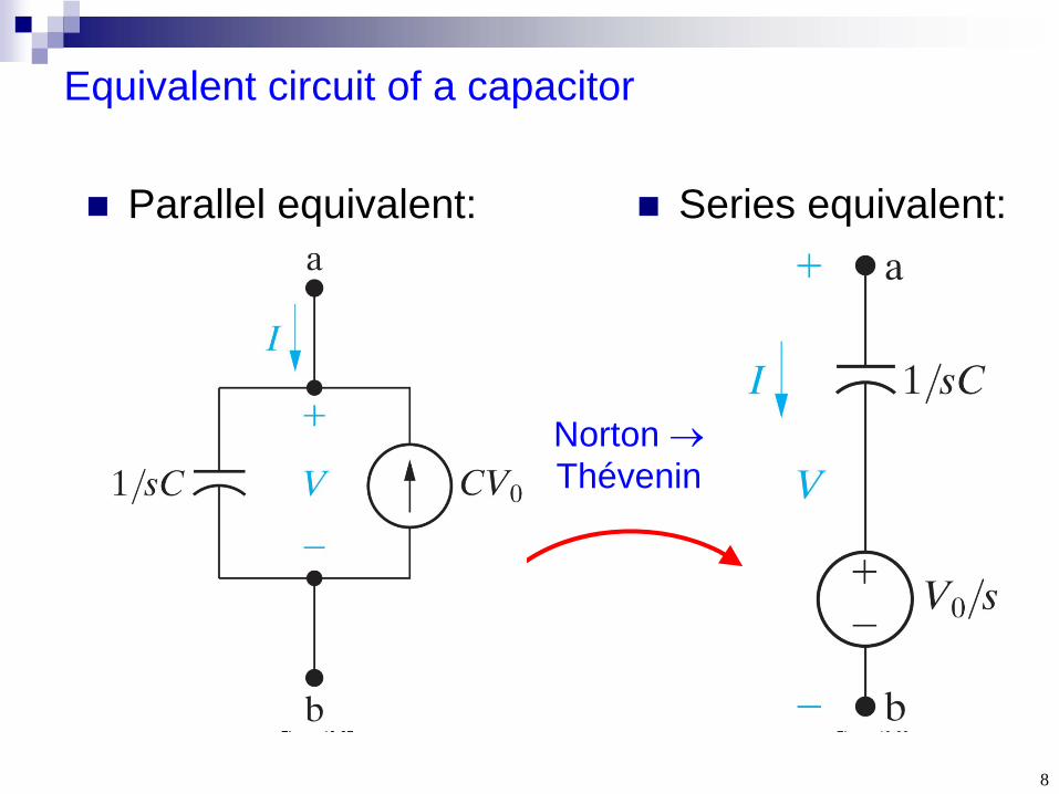
Equivalent circuit of a capacitor

Parallel equivalent:

Series equivalent:

Norton Thévenin

9

Circuit Analysis in the s Domain

1. Procedures2. Nature response of RC circuit3. Step response of RLC circuit4. Sinusoidal source5. MCM6. Superposition

Section 4.2, 4.3

10

How to analyze a circuit in the s-domain?

1. Replacing each circuit element with its s-domain equivalent. The initial energy in L or C is taken into account by adding independent source in series or parallel with the element impedance.

2. Writing & solving algebraic equations by the same circuit analysis techniques developed for resistive networks.

3. Obtaining the t-domain solutions by inverse Laplace transform.

11

Why to operate in the s-domain?

It is convenient in solving transient responses of linear, lumped parameter circuits, for the initial conditions have been incorporated into the equivalent circuit.

It is also useful for circuits with multiple essential nodes and meshes, for the simultaneous ODEs have been reduced to simultaneous algebraic equations.

It can correctly predict the impulsive response, which is more difficult in the t-domain (Sec. 4.8).

12

Nature response of an RC circuit (1)

Q: i(t), v(t)=?

.)(1

)( , 1000

RCsRV

RCsCVsIIR

sCI

sV

Replacing the charged capacitor by a Thévenin equivalent circuit in the s-domain.

KVL, algebraic equation & solution of I(s):


The t-domain solution is obtained by inverse Laplace transform:

).(

1)(

)(

)(0

1)(01

01

tueRV

sLe

RV

RCsRVLti

RCt

RCt

i(0+) = V0 /R, which is true for vC (0+) = vC (0-) = V0 .

i() = 0, which is true for capacitor becomes open (no loop current) in steady state.

4

14


To directly solve v(t), replacing the charged capacitor by a Norton equivalent in the s-domain.

.)(

)( , 10

0

RCsVsV

RVsCVCV

Solve V(s), perform inverse Laplace transform:

).()()( )( )(0

10

1 tRitueVRCsVLtv RCt

15

Step response of a parallel RLC (1)

iL (0-) = 0vC (0-) = 0

Q: iL (t)=?

16


KCL, algebraic equation & solution of V(s):

.)()(

)( , 112

LCsRCsCIsV

sLV

RVsCV

sI dcdc

Solve IL (s):

.)106.1()104.6(

1084.3

)()()()()(

942

7

112

1

sss

LCsRCssLCI

sLsVsI dc

L

17


Perform partial fraction expansion and inverse Laplace transform:

.s)(mA )k24k32(

12720)k24k32(

1272024)(

jsjss

sIL

.(mA) )( )k2432sin()k2424cos(24

(mA) )( 127k)24(cos4024

..)(20)(24)(

k)32(

k)32(

)k24(k)32(127

tutte

tute

cctueeetuti

t

t

tjtjL

18

Transient response due to a sinusoidal source (1)

For a parallel RLC circuit, replace the current source by a sinusoidal one: The algebraic equation changes:

.)()(

)()(

,)()(

)(

,

11222

1

11222

2

22

LCsRCsssLCI

sLVsI

LCsRCsssCIsV

ssII

sLV

RVsCV

mL

m

mg

).(cos)( tutIti mg

19

.)()(

)(*22

*11

jsK

jsK

jsK

jsKsIL

Driving frequency

Neper frequency

Damped frequency

).( cos2cos2)( 2211 tuKteKKtKti tL

Steady-state response (source)

Natural response (RLC parameters)

Transient response due to a sinusoidal source (2)

Perform partial fraction expansion and inverse Laplace transform:

20

Step response of a 2-mesh circuit (1)

i2 (0-) = 0i1 (0-) = 0

Q: i1 (t), i2 (t)=?

21


MCM, 2 algebraic equations & solutions:

)2(0)4810()(42

)1(336)(424.8

212

211

IsIIs

IIsI

.0

336109042

424.842

2

1

s

II

ss

.

124.1

24.87

121

21415

0336

109042424.842 1

2

1

sss

sssss

sII

22


Perform inverse Laplace

transform:

.A 15)48//42(

336)(1415)( 1221 tueeti tt

.A 74842

4215)(4.14.87)( 1222

tueeti tt

23

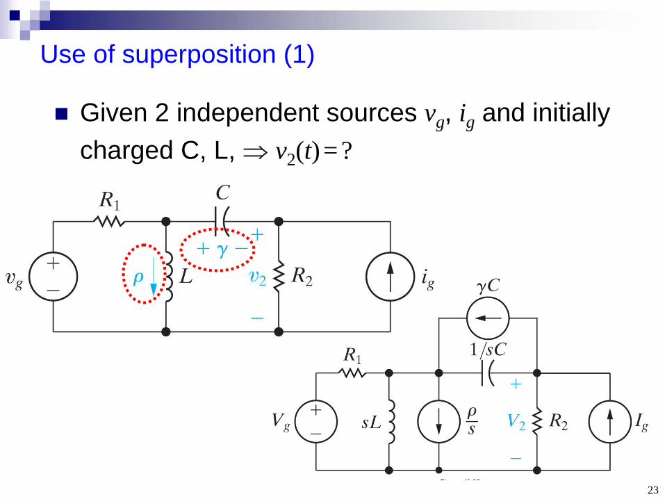
Use of superposition (1)

Given 2 independent sources vg , ig and initially charged C, L, v2 (t)=?

24

Use of superposition: Vg acts alone (2)

1 2

.01

,11

.0)(

,0)(

22

1

121

1

2

2112

1211

1

1

VsCR

VsC

RV

VsCVsCsLR

RV

sCVV

sCVV

sLV

RVV gg

25

Use of superposition (3)

.0

1

11

1

2

1

2212

1211

2

1

2

1

RVVV

YYYY

VV

sCR

sC

sCsCsLR

g

.2122211

1122 gV

YYYRYV

For convenience, define admittance matrix:

26

Use of superposition: Ig acts alone (4)

1 2

. ,0

2122211

112

2

1

2212

1211g

gI

YYYYV

IVV

YYYY

Same matrix Same denominator

27

Use of superposition: Energized L acts alone (5)

1 2

. ,0 2

122211

122

2

1

2212

1211

YYYsYV

sVV

YYYY

Same matrix Same denominator

28

Use of superposition: Energized C acts alone (6)

12

.)(

,

2122211

1211""2

""2

""1

2212

1211

YYYCYYV

CC

VV

YYYY

The total voltage is: .""22222 VVVVV

29

The Transfer Function and Natural Response

Section 4.4, 4.5

30

What is the transfer function of a circuit?

The ratio of a circuit’s output to its input in the s-domain:

)()()(

sXsYsH

A single circuit may have many transfer functions, each corresponds to some specific choices of input and output.

31

Poles and zeros of transfer function

For linear and lumped-parameter circuits, H(s) is always a rational function of s.

Poles and zeros always appear in complex conjugate pairs.

The poles must lie in the left half of the s-plane if bounded input leads to bounded output.

Re

Im

32

Example: Series RLC circuit

If the output is the loop current I:

.1)(

1)( 21

sRCLCs

sCsCsLRV

IsHg

If the output is the capacitor voltage V:

.1

1)(

)()( 21

1

sRCLCssCsLRsC

VVsH

g

input

33

How do poles, zeros influence the solution?

Since Y(s) =H(s) X(s), the partial fraction expansion of the output Y(s) yields a term K/(s-a) for each pole s =a of H(s) or X(s).

The functional forms of the transient (natural) and steady-state responses ytr (t) and yss (t) are determined by the poles of H(s) and X(s), respectively.

The partial fraction coefficients of Ytr (s) and Yss (s) are determined by both H(s) and X(s).

34

50tu(t)

50/s2

Q: vo (t)=?

Example 4.2: Linear ramp excitation (1)

35

Only one essential node, use NVM:

,01005.02501000 6

s

Vs

VVV oogo

.105.26000)5000(1000)(

72

sss

VVsH

g

o

H(s) has 2 complex conjugate poles:

Vg (s) = 50/s2 has 1 repeated real pole: s = 0(2).

.40003000 js

Example 4.2 (2)

36

The total response in the s-domain is:

).(10410

)()80000,4cos(105)(4

000,33

tut

tuteyytv tsstro

sstrgo YYsssssVsHsV

722

4

105.26000)5000(105)()()(

The total response in the t-domain:

poles of H(s): -3k

j4k pole of Vg (s): 0(2)

expansion coefficients depend on H(s) & Vg (s)

.1041040003000

80105540003000801055 4

2

44

ssjsjs

Example 4.2 (3)

37

Steady state component yss (t)

Total response

= 0.33 ms, impact of ytr (t)

Example 4.2 (4)

38

The Transfer Function and the Convolution Integral

1. Impulse response2. Time invariant3. Convolution integral4. Memory of circuit

Section 4.6

39

Impulse response

If the input to a linear, lumped-parameter circuit is an impulse (t), the output function h(t) is called impulse response, which happens to be the natural response of the circuit:

).()()()(

),(1)()( ,1)()(11 thsHLsYLty

sHsHsYtLsX

The application of an impulse source is equivalent to suddenly storing energy in the circuit. The subsequent release of this energy gives rise to the natural response.

40

Time invariant

For a linear, lumped-parameter circuit, delaying the input x(t) by simply delays the response y(t) by as well (time invariant):

).()(

)(),(),(

),()()(),()(),(),()()(),(

11

tuty

sYLsYLty

sYesXsHesXsHsYsXetutxLsX

tt

ss

s

41

Motivation of working in the time domain

The properties of impulse response and time- invariance allow one to calculate the output function y(t) of a “linear and time invariant (LTI)” circuit in the t-domain only.

This is beneficial when x(t), h(t) are known only through experimental data.

42

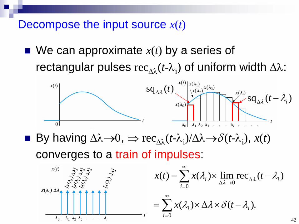
Decompose the input source x(t)

We can approximate x(t) by a series of rectangular pulses rec

(t-i ) of uniform width :

By having , rec

(t-i )/ (t-i ), x(t) converges to a train of impulses:

)(sq it

)(sq t

.)()(

)(reclim)()(

0

0 0

iii

iii

tx

txtx

43

Synthesize the output y(t) (1)

Since the circuit is LTI:

.)()(

)()(

0

0

iii

iii

thx

tx

;)()(),()(

),()(

tyatxatht

tht

iiii

ii

44

As , summation integration:

.)()()()()(0

dthxdthxty

if x(t) extends (-, )

By change of variable u= t-,

.)()()(

duuhutxty

The output of an LTI circuit is the convolution of input and the impulse response of the circuit:

.)()()()(

)()()(

dhtxdthx

thtxty

Synthesize the output y(t) (2)

45

Convolution of a causal circuit

For physically realizable circuit, no response can occur prior to the input excitation (causal), {h(t) =0 for t <0}.

Excitation is turned on at t =0, {x(t)=0 for t <0}.

.)()(

)()()(

0

t

dhtx

thtxty

46

Effect of x(t) is weighted by h(t)

The convolution integral

If h(t) is monotonically decreasing, the highest weight is given to the present x(t).

t0

t

dhtxty0

)()()(

shows that the value of y(t) is the weighted average of x(t) from t =0 to t = t [from

= t to =0 for x(t-)].

47

Memory of the circuit

.)()()(0 t

dhtxty

implies that the circuit has a memory over a finite interval t =[t-T,t].

T

If h(t) only lasts from t =0 to t =T, the convolution integral

If h(t) =(t), no memory, output at t only depends on x(t), y(t) =x(t)*(t) =x(t), no distortion.

48

.1

1)( ,1

1

sV

VsHVs

Vi

oio

).(1

1)( 1 tues

Lth t

Q: vo (t)=?

Example 4.3: RL driven by a trapezoidal source (1)

49

.)()()(0 t

io dhtvtv

Separate into 3 intervals:

Example 4.3 (2)

50

Since the circuit has certain memory, vo (t) has some distortion with respect to vi (t).

Example 4.3 (3)

51

The Transfer Function and the Steady-State Sinusoidal Response

Section 4.7

52

How to get sinusoidal steady-state response by H(s)?

In Chapters 9-11, we used phasor analysis to get steady-state response yss (t) due to a sinusoidal input

If we know H(s), yss (t) must be:

.)()()( where

,)(cos)()()(

j

js

ss

ejHsHjH

tAjHty

The changes of amplitude and phase depend on the sampling of H(s) along the imaginary axis.

.cos)( tAtx

53

Proof

.sinsincoscoscos)( tAtAtAtx

.sincossincos)( 222222

s

sAs

As

sAsX

),()(sincos)()()()( 22 sYsYs

sAsHsXsHsY sstr

.)(cos)(..)(2

)()(

)(1

tjHAcc

jsAeejH

Ltyjj

ss

.2)(

2sincos)(sincos)(

))(( ,)( where 1

*11

j

js

jsss

AejHj

jAjHjs

sAsH

jssYKjs

Kjs

KsY

54

Obtain H(s) from H( j)

We can reverse the process: determine H( j) experimentally, then construct H(s) from the data (not always possible).

Once we know H(s), we can find the response to other excitation sources.

55

The Impulse Function in Circuit Analysis

Section 4.8

56

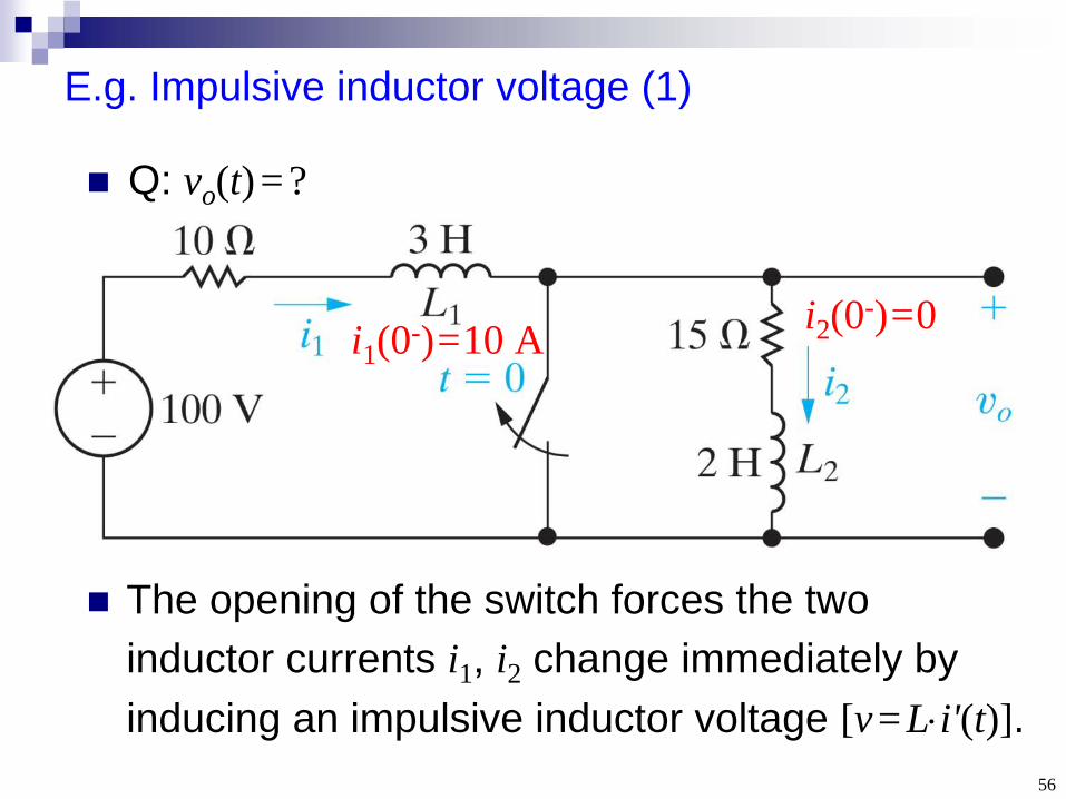
E.g. Impulsive inductor voltage (1)

The opening of the switch forces the two inductor currents i1 , i2 change immediately by inducing an impulsive inductor voltage [v=Li'(t)].

i1 (0-)=10 A i2 (0-)=0

Q: vo (t)=?

57

E.g. Equivalent circuit & solution in the s-domain (2)

.5

106012)5(

)150656(2)(2

0

ssss

sssVimproper rational

initial current

,0215310

)30100( 00

s

VssV

58

E.g. Solutions in the t-domain (3)

).()1060()(125

106012)( 510 tuet

ssLtv t

To verify whether this solution vo (t) is correct, we need to solve i(t) as well.

).()24()( ,5

24215310

30100)( 5 tuetissss

ssI t

jump

jump

59

Impulsive inductor voltage (4)

The jump of i2 (t) from 0 to 6 A causes , contributing to a voltage impulse

After t > 0+,

consistent with that solved by Laplace transform.

)(6)(2 tti

,1060)10(2)24(15

)()H2()()15()(555

22ttt

o

eee

tititv

).(12)(22 ttiL

60

Key points

How to represent the initial energy of L, C in the s-domain?

Why the functional forms of natural and steady- state responses are determined by the poles of transfer function H(s) and excitation source X(s), respectively?

Why the output of an LTI circuit is the convolution of the input and impulse response? How to interpret the memory of a circuit by convolution?

61

Practical Perspective Voltage Surges

62

Why can a voltage surge occur?

Q: Why a voltage surge is created when a load is switched off?

Model: A sinusoidal voltage source drives three loads, where Rb is switched off at t =0.

Since i2 (t) cannot change abruptly, i1 (t) will jump by the amount of i3 (0-), voltage surge occurs.

63

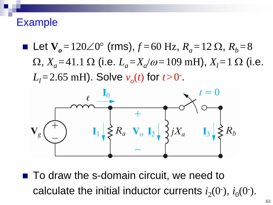
Example

Let Vo =1200

(rms), f =60 Hz, Ra =12 , Rb =8 , Xa =41.1

(i.e. La =Xa /=109 mH), Xl =1

(i.e.

Ll =2.65 mH). Solve vo (t) for t >0-.

To draw the s-domain circuit, we need to calculate the initial inductor currents i2 (0-), i0 (0-).

64

Steady-state before the switching

The three branch currents (rms phasors) are:

I1 =Vo /Ra =(1200)/(12 )=100

A,

I2 =Vo /(jXa ) = (1200)/(j41.1 )=2.92-90

A,

I3 =Vo /Rb =(1200)/(8 )=150

A,

The line current is: I0 = I1 + I2 + I3 =25.2-6.65

A.

Source voltage: Vg =Vo + I0 (jXl )=125-11.5

V.

The two initial inductor currents at t =0- are:

i2 (t)=2.92(2)cos(120t-90), i2 (0-)=0;

i0 (t)=25.2(2)cos(120t-6.65), i0 (0-) =35.4 A.

65

S-domain analysis

The s-domain circuit is:

By NVM:

(Ll = 2.65 mH)

(I0 = 35.4 A)

(12 ) (La = 109 mH)

,00

a

o

a

o

l

glo

sLV

RV

sLVILV

120

85.686120

85.6861475253

)()( 0

jsjssLLLLRsRIsVLR

Vlalaa

aglao

Vg = 125- 11.5

V (rms)

66

Inverse Laplace transform

Given ,120

85.686120

85.6861475253)(

jsjsssVo

).()85.6120cos(173 253)( 1475 tutetv to

0

Two Port Network

1

Two Post Network:

Two Post Network

+

-

+

-

Post-IInput port

Port-IIOutput port

Fig.1

A network which has two terminals (one port) on the one side and another two terminals on

the opposite side forms a two port network. One port functions as input and the other as

output to the network.

The networks may composed of active or passive elements, but we are not concerned with its

internal functioning and simple we assumed as a black box

From above fig.1 it is noted that there are four variable V1,I1,V2,I2 of the four , any two can be

dependent and other two independent, which gives rise to different parameters-

(a) Impedance parameters or Z parameters.

(b)Admittance parameters or Y parameters.

(C) Hybrid parameters or h parameters

(d)Transmission parameters.

(2) Reason why to study two port – network:

(a) Such networks are useful in communication, control system, power systems

and electronics.

(b) Knowing the parameters of a two – port network enables us to treat it as a

“black box” when embedded within a larger network.

(a) Impedance parameters or Z parameters.

Linear Network

+

-

+

-

Fig.2

2

Impedance parameters are commonly used in the synthesis of filters and also useful in the

design and analysis of impedance matching networks and power distribution networks.

V1, V2 are dependent variables.

II , I2 are independent variables.

The defining equations are-

...........(1)1 11 1 12 2............(2)2 21 1 22 2

V z I z I

V z I z I

= +

= +

In matrix form as:

11 121 1

21 222 2

z zV I

z zV I

= ………….. ……..(3)

To obtain Z parameters, we alternatively open circuit the output and input ports.

Thus-

111

1 02

221

1 02

Vz

II

Vz

II

==

==

11 2

2 01

22 2

2 01

Vz

II

Vz

II

==

==

These parameters are as follows:

z11 Open circuit input impedance

z12 Open circuit transfer impedance from port 1 to port 2

z21 Open circuit transfer impedance from port 2 to port 1

z22 Open circuit output impedance

When z11=z22, the network is said to be symmetrical.

• When the network is linear and has no dependent sources, the transfer impedances

are equal (z12=z21), the network is said to be reciprocal.

3

• This means that if the input and output are switched, the transfer impedances remain

the same.

Any two-port network that is composed entirely of resistors, capacitors, and inductors

must be reciprocal

Since, the Z parameters are obtained by opening the input or output port, they are also called

the open circuit impedances.

Z11 and Z22 are called driving point impedances and Z12 and Z21 are called transfer

impedances.

Z- Parameters for a T-Network-

-

+

-

Fig.3

Z11 = ZA +ZC Z12 = Z21 =Zc Z22 =ZB +ZC

Network in which, Z12 = Z21 as in case in above T network are called reciprocal networks.

If ZA =ZB, the network is symmetrical.

Equivalent circuit for the Z parameters is here under-

4

+ +

1V2V

11Z 22Z

12 2Z I 21 1Z I

1I2I

Fig.4

(b)Admittance parameters or Y parameters.

Linear Network

+

-

+

-

Fig.2

Fig.5

Y – Parameter also called admittance parameter and the units is Siemens (S).

V1, V2 are independent variables.

II , I2 are dependent variables.

The defining equations are-

11 121 1

21 222 2

y yI V

y yI V

=

It is represented as a circuit as follows-

5

1V2V

11Y

22Y12 2VY

21 1VY

1I2I

Fig.6

This is a voltage controlled (dependent) current source (VCCS)

In the matrix form-

11 121 1

21 222 2

y yI V

y yI V

=

To obtain the Y parameters, we alternatively short circuited the input and output ports. Thus-

111

1 02

221

1 02

IY

VV

IY

VV

==

==

112

2 01

222

2 01

IY

VV

IY

VV

==

==

These parameters are as follows:

y11 Short circuit input admittance

y12 Short circuit transfer admittance from port 1 to port 2

y21 Short circuit transfer admittance from port 2 to port 1

y22 Short circuit output admittance

The impedance and admittance parameters are collectively called the immitance

parameters.

6

Since, the Y parameters are obtained by short circuiting the input or output, therefore they

are also called the short circuit admittance parameters.

Y parameters for π network-

1V 2V

CY

AYBY

1I 2I

Fig.7

Y parameters can also be obtained from the Z parameters-

[V] = [Z][I] or, [I] = [Z]-1[V]

Therefore-

111 12 22 12

21 22 21 11

Y Y Z Z

ZY Y Z Z

−=

∆ −

Where Z∆ = determinant of Z

Reciprocal network

Symmetrical Network condition

(C) Hybrid parameters or h parameters

7

Linear Network

+

-

+

-

Fig.2

Fig.8

I1, V2 are independent variables.

I2 ,V1 are dependent variables the, defining equations are-

1 11 1 12 2

2 21 1 22 2

V h I h V

I h I h V

= +

= +

In the matrix form-

11 12

21 222

11

2

Ih

Vh

V h

hI

=

The h terms are known as the hybrid parameters, or simply h-parameters. The name comes

from the fact that they are a hybrid combination of ratios. These parameters tend to be much

easier to measure than the z or y parameters. They are particularly useful for characterizing

transistors.Transformers too can be characterized by the h parameters.

The h parameters are obtained from above equations by setting V2=0 i.e output port short

circuited and I1=0 i.e input open circuited.

1 111 12

1 20 02 1

2 221 22

1 20 02 1

V Vh h

I VV I

I Ih h

I VV I

= == =

= == =

The parameters h11, h12, h21, and h22represent an impedance, a voltage gain, a current gain,

and an admittance respectively.

8

The h-parameters correspond to:

h11 Short circuit input impedance

h12 Open circuit reverse voltage gain

h21 Short circuit forward current gain

h22 Open circuit output admittance

In a reciprocal network, h12=-h21.

The equivalent network is shown below:

The inverse of hybrid parameters are called g parameters, inverse hybrid parameters-

1 11 1 12 2

2 21 1 22 2

I g V g I

V g V g I

= +

= +

The values of the g parameters are determined as:

1 111 12

1 20 02 1

2 221 22

1 20 02 1

I Ig g

V II V

V Vg g

V II V

= == =

= == =

The equivalent model is shown below:

+

1V2V

12 2h V 21 1h I

11h

22h

Fig.9

The g parameters correspond to:

9

g11 Open circuit input admittance

g12 Short circuit reverse current gain

g21 Open circuit forward voltage gain

g22 Short circuit output impedance

(d)Transmission parameters or ABCD parameters:

Linear Network

+

-

+

-

Fig.2

Fig.10

T – parameter or ABCD – parameter is a set of parameters relates the variables at the

input port to those at the output port.

T – parameter also called transmission parameters because this parameter are useful in

the analysis of transmission lines because they express sending – end variables (V1 and I1)

in terms of the receiving – end variables (V2 and -I2).

The equation is:

.......(1)1 2 2

.......(2)1 2 2

V AV BI

I CV DI

= −

= −

In matrix form is:

1 2

1 2

V VA B

I IC D

=−

The T – parameter that we want determine are A, B, C and D where A and D are

dimensionless, B is in ohm (Ω) and C is in Siemens (S).

The values can be evaluated by setting

10

I2 = 0 (input port open – circuit)

V2 = 0 (output port short circuit)

Thus;

1

2 02

1

2 02

VA

VI

IC

VI

==

==

1

2 02

1

2 02

VB

IV

ID

IV

==

==

In term of the transmission parameter, a network is reciprocal if;

AD-BC=1 and for symmetrical A=D.

Condition for reciprocity and symmetry:

Parameters Condition of Reciprocity Condition of symmetry

[Z] Z12=Z21 z11=z22

[Y] Y12=Y21 Y11=Y22

[h] h12=-h21 h11h22-h12h21=1

[g] g12=-g21 g11g22-g12g21=1

[ABCD] AD-BC=1 A=D

Interconnections of Networks

Often it is worthwhile to break up a complex network into smaller parts.

The sub-network may be modeled as interconnected two port networks.

From this perspective, two port networks can be seen as building blocks for constructing

a more complex network.

These connections may be in series, parallel, or cascaded.

(1)Series Connection

Two port networks with ABCD parameters are A,B,C,D and A’,B’,C’,D’ are connected in

series as shown in fig below-

11

'A 'B

'D'C

2V1V '2V'

1V

1I 2I '1I

'2I

Fig.11

1 2

1 2

V VA B

I IC D

=−

and

' '' '

' ' ' '

1 2

1 2

V VA B

I C D I

=−

Here I2= '

1I and V2= '1V

'' '

' ' '

1 2

1 2

V VA B A B

I C D C D I

=−

Thus the overall transmission matrix for two port networks in tandem is the matrix

product of individual transmission network matrix.

When two port networks are connected in series, the Z parameter of the combination is

equal to the sum of the individual Z parameters.

11 12 11 1211 12

21 22 21 22 21 22

Z ZZ ZZ Z

Z Z Z Z Z Z

a a b b

a a b b

= +

(2)Parallel Connection

Two port networks are in parallel when their port voltages are equal and the port

currents of the larger network are the sums of the individual port currents. Consider the

network shown-

12

1V

+

--

2VNetwork

a

Network

b

1I 2I2aI1aI

2aI2bI

2bV1bV

2aV1aV

Fig.12

Va=Vb=V, I1=Ia1+Ib1, I2=Ia2+Ib2

[I]=[IYaI+IYbI][V]. the Y parameter of the parallel network is equal to the sum of the

individual network’s Y parameter.

[Y]=[Ya]+[Yb]

(3)Series-Parallel Connection:

In this connection the input ports are connected in series while the output ports are

connected in parallel. The connection requires that-

V1=V1a+V1b, I1=I1a=I1b and V2=V2a=V2b, I2=I1a+I2b

1V 2V

1I 2I2aI1aI

1bI2bI

2bV1bV

2aV1aV

Fig.13

The overall h-parameters of the combined series-parallel connection can be obtained by

adding their individual h-parameters.

13

So, overall we have- 11 12 11 1211 12

21 22 21 22 21 22

h hh hh h a a b bh h h h h ha a b b

= +

(4) Parallel-Series connection.

In this connection the input ports are connected in parallel while the output ports are

connected in series. The connection requires that-

V1=V1a=V1b, I1=I1a+I1b and V2=V2a+V2b, I2=I1a+I2b

1V

+

-

-

2V

Network

a

Network

b

1I 2I2aI1aI

1bI2bI

2bV1bV

2aV1aV

Fig.14

The overall inverse h-parameters or g-parameters of the combined parallel series

connection can be obtained by adding their individual g-parameters.

So, overall we have-

11 12 11 1211 12

21 22 21 22 21 22

g gg gg g

g g g g g g

a a b b

a a b b

= +

Image Impedance:

14

In a two port network, if two impedances Zi1 and Zi2 are such that Zi1 is the driving point

impedance at port 1 with impedance Zi2 connected across port 2 and Zi2 is the driving

point impedance at port2 with impedance Zi1 connected across port1, then impedances Zi1

and zi2 are called the image impedances of the network.

For symmetrical network image impedances are equal to each other i.e Zi1=Zi2 and is

called the characteristic or iterative impedance Zc.

Two port

Network1iZ 2V

1V2iZ

2I1I

Fig.a

1iZ 2V1V 2iZ

2I1I

In fig.a 11

1

VZi I

= =driving point impedance at port 1.

In fig.b 2

22

VZi I= = driving point impedance at port 2.

T to π Transformation:

cY

bYaY

1Z 2Z

3Z

15

Impedances Z1, Z2, and Z3 of the above fig.a T network are known and it is require to

calculate equivalent admittances Ya , Yb and Yc of the π network in the fig.b

2

1 2 2 3 3 1

ZYa Z Z Z Z Z Z

=+ +

, 1

1 2 2 3 3 1b

ZYZ Z Z Z Z Z

=+ +

and 3

1 2 2 3 3 1c

ZY

Z Z Z Z Z Z=

+ +

π to T Transformation:

cY

bYaY

1Z 2Z

3Z

In this case, admittances Ya,Yb ,and Yc of the above fig.a π network are known and it is

require to calculate equivalent impedances Z1 ,Z2 and Z3 of the T network in the fig.b

1

YbZY Y Y Y Y Ya c c ab b

=+ +

, 2aY

ZY Y Y Y Y Ya c c ab b

=+ +

and 3cY

ZY Y Y Y Y Ya c c ab b

=+ +

Chapter 4 The Laplace Transform in Circuit Analysis

Documents