CHAPTER 4 LYAPUNOV EXPONENT - Shodhgangashodhganga.inflibnet.ac.in/bitstream/10603/7179/12/12_chapter 4.pdf · 68 gives the average exponential rate of divergence or convergence of

63

CHAPTER 4

LYAPUNOV EXPONENT

64

4.1 Introduction

Convincing evidence for deterministic chaos has come from a

variety of recent experiments on dissipative nonlinear systems[1-24] ;

therefore , the question of detecting and quantifying chaos has become an

important one . The spectrum of Lyapunov exponents has proven to be

the most useful dynamical diagnostic for chaotic system. Lyapunov

exponents are the average exponential rates of divergence or

convergence of nearby orbits in phase space[25-31]. Since nearby orbits

corresponds to nearly identical states, exponential orbital divergence

means that systems whose initial differences is not possible to resolve

will soon behave quite differently and predictive ability will be rapidly

lost. Any system containing atleast one positive Lyapunov exponents is

defined to be chaotic , with the magnitude of the exponent reflecting the

time scale on which system dynamics become unpredictable[32-37].

For systems whose equations of motion are explicitly known there

is a straightforward technique for computing a complete Lyapunov

exponent spectrum. This method cannot be applied directly to experimental

data. A technique is described which for the first time yields estimates of

the non-negative Lyapunov exponent from the finite amounts of

experimental data[38-42].

It is known that a system‟s behavior is chaotic if its average

Lyapunov exponent is a positive number. In this study, we will describe

the calculation of the Lyapunov exponent from a one dimensional time-

series data . The series x(t0) ,x(t1) ,x(t2),……………. is leveled as x0 ,x1 ,x2

,…… For the sake of simplicity, it is assumed, as is usually the case, that

the time intervals between samples can be written as

65

tn – t0 = nτ (4.1)

where τ is the time interval between samples . If the system is behaving

chaotically , the divergence of nearby trajectories will manifest itself in

the following way :

If some value is selected from the sequences of x‟s , say xi , and

then search the sequence for another x value , say , xj , that is close to xj

, then the sequence of differences given by

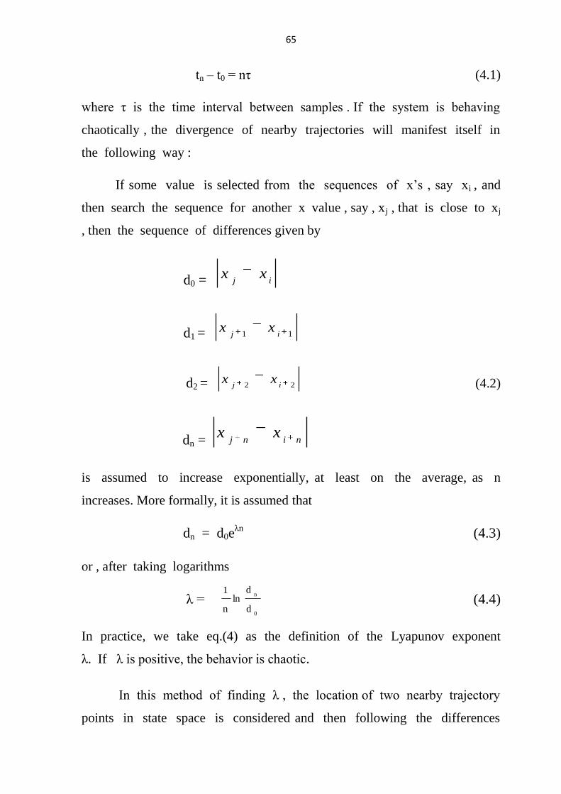
d0 = ijxx

d1 = 11 ijxx

d2 = 22 ijxx (4.2)

dn = ninjxx

is assumed to increase exponentially, at least on the average, as n

increases. More formally, it is assumed that

dn = d0eλn

(4.3)

or , after taking logarithms

λ = (4.4)

In practice, we take eq.(4) as the definition of the Lyapunov exponent

λ. If λ is positive, the behavior is chaotic.

In this method of finding λ , the location of two nearby trajectory

points in state space is considered and then following the differences

0

n

d

dln

n

1

66

between the two trajectories that follow each of these “initial” points the

divergence is determined. Consider two points in a space, x0 and x0 + Δx0 ,

each of which will generate an orbit in that space using some equation or

system of equations. These orbits can be thought of as parametric functions of

a variable that is something like time. If one of the orbits is considered as a

reference orbit, then the separation between the two orbits will also be a

function of time. Because sensitive dependence can arise only in some portions

of a system, this separation is also a function of the location of the initial value

and has the form Δx (x0, t). In a system with attracting fixed points or

attracting periodic points, Δx(x0, t) diminishes asymptotically with time. If a

system is unstable, like pins balanced on their points, then the orbits diverge

exponentially for a while, but eventually settle down. For chaotic points, the

function Δx(x0, t) will behave erratically.

It is thus useful to study the mean exponential rate of divergence of two

initially close orbits using the formula

λ = Limt

t

1

ln 0

0),(

X

tXx

(4.5)

The number "λ", called the Lyapunov exponent is useful for

distinguishing among the various types of orbits. It works for discrete as well

as continuous systems. The following cases are possible:

λ < 0 : The orbit attracts to a stable fixed point or stable periodic orbit.

Negative Lyapunov exponents are characteristic of dissipative or non-

conservative systems (the damped harmonic oscillator for instance). Such

systems exhibit asymptotic stability; the more negative the exponent, the

greater the stability. Superstable fixed points and superstable periodic points

have a Lyapunov exponent of λ = −∞. This is something akin to a critically

00

X

67

damped oscillator in that the system heads towards its equilibrium point as

quickly as possible.

λ = 0: The orbit is a neutral fixed point (or an eventually fixed point). A

Lyapunov exponent of zero indicates that the system is in some sort of steady

state mode. A physical system with this exponent is conservative. Such

systems exhibit Lyapunov stability. The orbits in this situation would maintain

a constant separation, like two flecks of dust fixed in place on a rotating

record.

λ > 0: The orbit is unstable and chaotic. Nearby points, no matter how close,

shall diverge to any arbitrary separation. All neighborhoods in the phase space

will eventually be visited. These points are said to be unstable. For a discrete

system, the orbits will look like snow on a television set. This does not

preclude any organization as a pattern may emerge. A physical example can be

found in Brownian motion. Although the system is deterministic, there is no

order to the orbit that ensues.

The Lyapunov exponent can also be found using the formula

λ = limN

N

1

N

1n

log2

n

1n

dx

dx

(4.6)

This number can be calculated to a reasonable degree of accuracy by

choosing a suitably large "N".

As the Lyapunov exponent measures the rate of divergence or

convergence of two nearby initial points of a dynamical system. In other

words, A Lyapunov exponent is a measure of the rate of attraction to and

repulsion from a fixed point in state space. Lyapunov exponent tell us the rate

of divergence of nearby trajectories – a key component of chaotic dynamics. It

68

gives the average exponential rate of divergence or convergence of the nearby

orbits in the phase space. Because the presence of a positive Lyapunov

exponent implies the divergence of the nearby trajectories, a system having at

least one positive Lyapunov exponent is often considered to be chaotic.

As linear methods interpret all regular structure in a data set, such as a

dominant frequency, through linear correlations, this means, in brief, that the

intrinsic dynamics of the system are governed by the linear paradigm that

small causes lead to small effects. Since linear equations can only lead to

exponentially decaying (or growing) or (damped) periodically oscillating

solutions, all irregular behavior of the system has to be attributed to some

random external input to the system. But results of chaos theory has proved

that random input is not the only possible source of irregularity in a system's

output: nonlinear, chaotic systems can produce very irregular data with purely

deterministic equations of motion in an autonomous way, i.e., without time

dependent inputs. Of course, a system which has both, nonlinearity and

random input, will most likely produce irregular data as well. Lyapunov

exponent can be used as a diagnostic tool to distinguish chaotic data from a

random one.

4.3 Data Analysis and Results

Lyapunov exponent of index values, P/E values and values of different

indices with its DFA profiles are plotted at different time. Variation in P/E

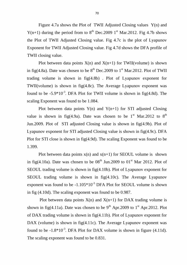
value of NIFTY(X(0)) from 7th

Jan 1999 to 7th sep. 2001 is plotted in fig

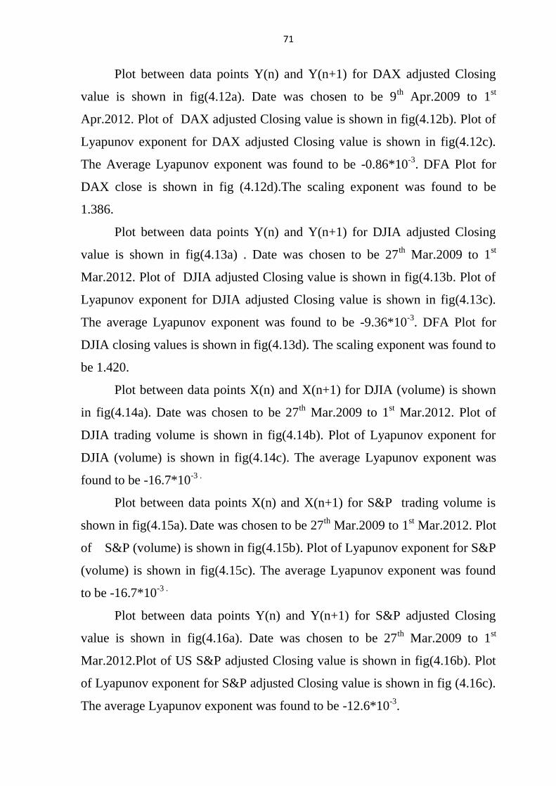
(4.1a). The Graph of Lyapunov exponent for P/E value of NIFTY(X(0)) is

plotted in fig (4.1b). The average Lyapunov exponent was found to be -9.715 x

10-3

. Graph between for P/E values of NIFTY X(n) and X(n+1) is plotted in fig

(4.1c) . Date was chosen to be 7th

Jan.1999 to 7th

sep.2001.

69

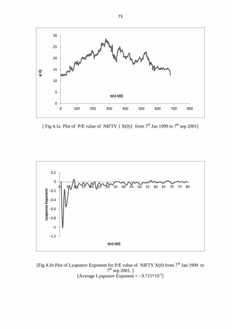
Variation in P/E value of NIFTY(Y(0)) is plotted in fig (4.2a). Date

was chosen to be 17th Sep. 2001 to 1

st Jan.2004. Graph of Lyapunov exponent

for P/E value of NIFTY(Y(0)) is plotted in fig (4.2b). The Average Lyapunov

exponent was found to be -1.25 x 10-3

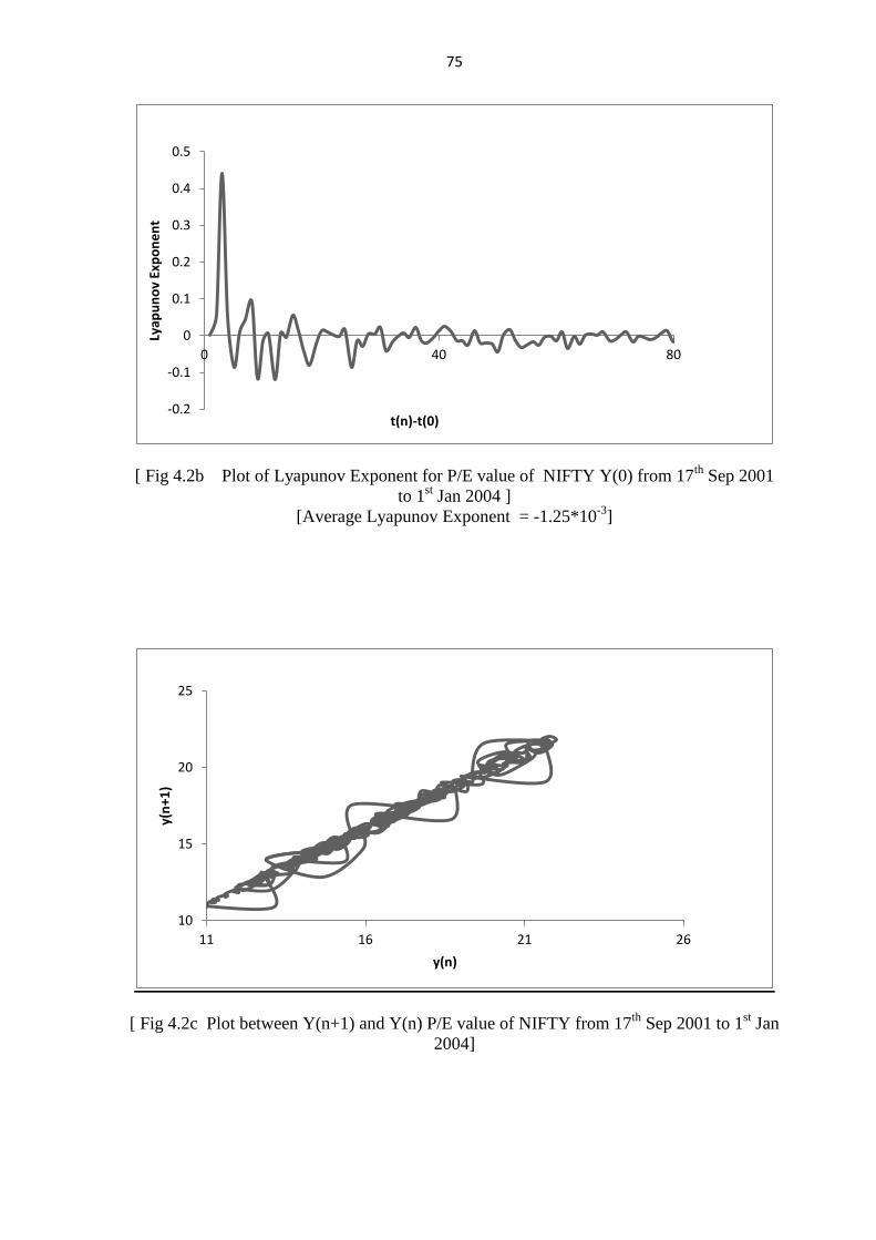
. Graph between P/E value of NIFTY

Y(n) and Y(n+1) is plotted in fig (4.2c).

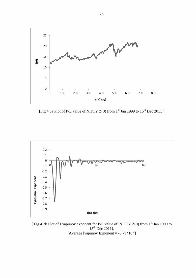
Variation in P/E value of NIFTY Z(0) is plotted in fig(4.3a). The period

chosen was from 1st Jan.1999 to 15

th Dec.2011. Graph of Lyapunov exponent

for P/E value of NIFTY (Z(0)) is plotted in fig (4.3b). Graph between P/E

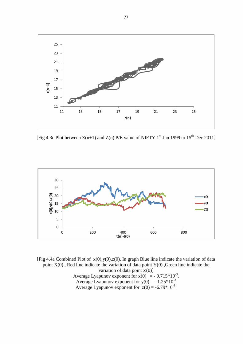
value of NIFTY Z(n) and Z(n+1) is plotted in fig (4.3c) for the same period.

Variation in P/E values of NIFTY from 7th

Jan.1999 to 9th

Feb.2007 is

plotted in fig(4.4a). Fig 4(.4b) shows the Plots of Lyapunov exponents for X(0)

Y(0),Z(0) 7th

between Jan.1999 to 9th

Feb.2007.

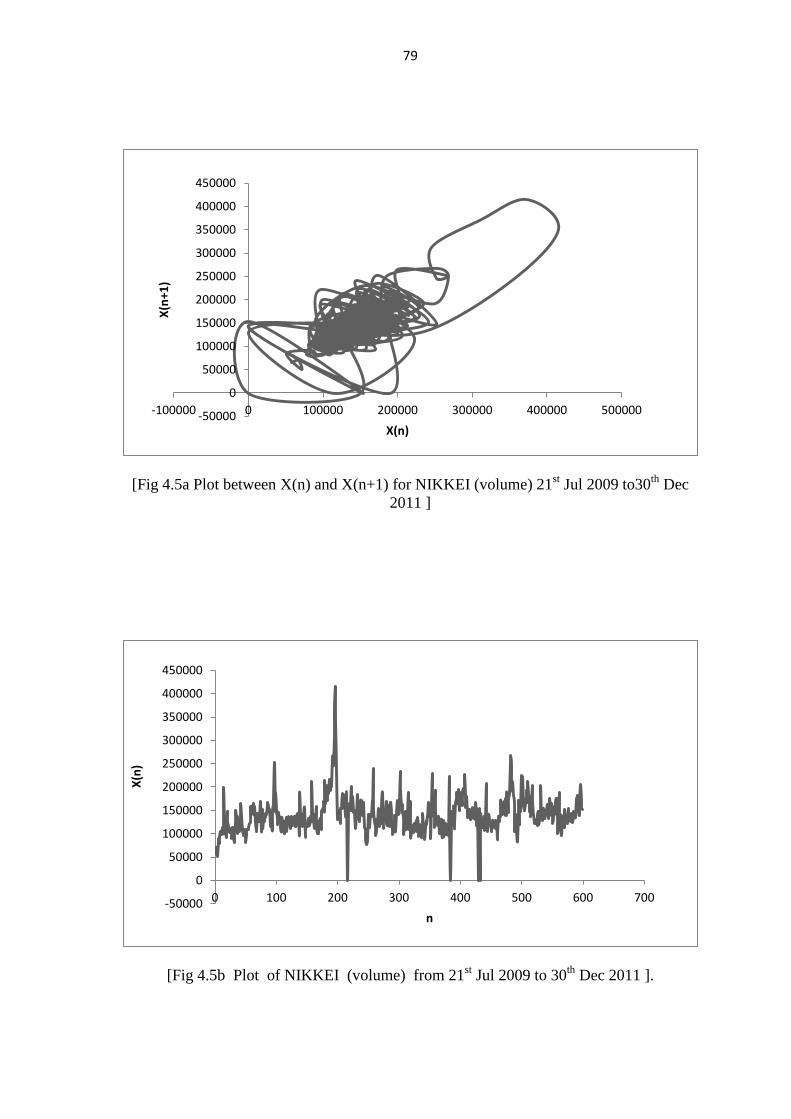
Phase plot between data points x(n) and x(n+1) for NIKKEI volume is

shown in fig(4.5a). Date was chosen to be 21st Jul.2009 to 30

th Dec.2011. Plot

between number of data points n and data points X(n) for NIKKI(volume) is

shown in fig(4.5b). Date was chosen to be 21st Jul.2009 to 30

th Dec.2011. Plot

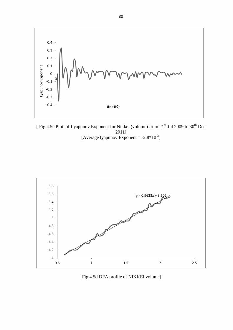
of Lyapunov exponent for NIKKI(volume) is shown in fig(4.5c). The Average

Lyapunov exponent was found to be 2.8*10-3

. Date was chosen to be 21st

Jul.2009 to 30th Dec.2011. DFA Plot for NIKKI volume is shown in fig (4.5d).

The scaling Exponent was found to be 0.962.

Plot between data points x(n) and x(n+1) for NIKKI (Adjusted Closing

value) is shown in fig(4.6a). Date was chosen to be from 21st Jul.2009 to 30

th

Dec.2011. Plot between number of data points n and data points X(n) for

NIKKI(Adjusted volume) is shown in fig(4.6b) for the same period. Figure

(4.6c) shows the Plot of Lyapunov exponent for NIKKEI Adjusted Closing

value. Average Lyapunov exponent is calculated to be -0.0104*10-3.

Fig (4.6d)

shows the DFA profile of NIKKEI closing value The scaling Exponent was

found to be 1.385.

70

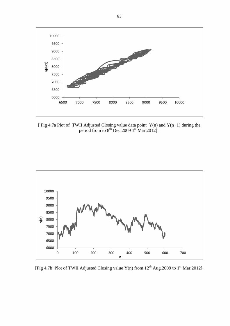
Figure 4.7a shows the Plot of TWII Adjusted Closing values Y(n) and

Y(n+1) during the period from to 8th

Dec.2009 1st Mar.2012. Fig 4.7b shows

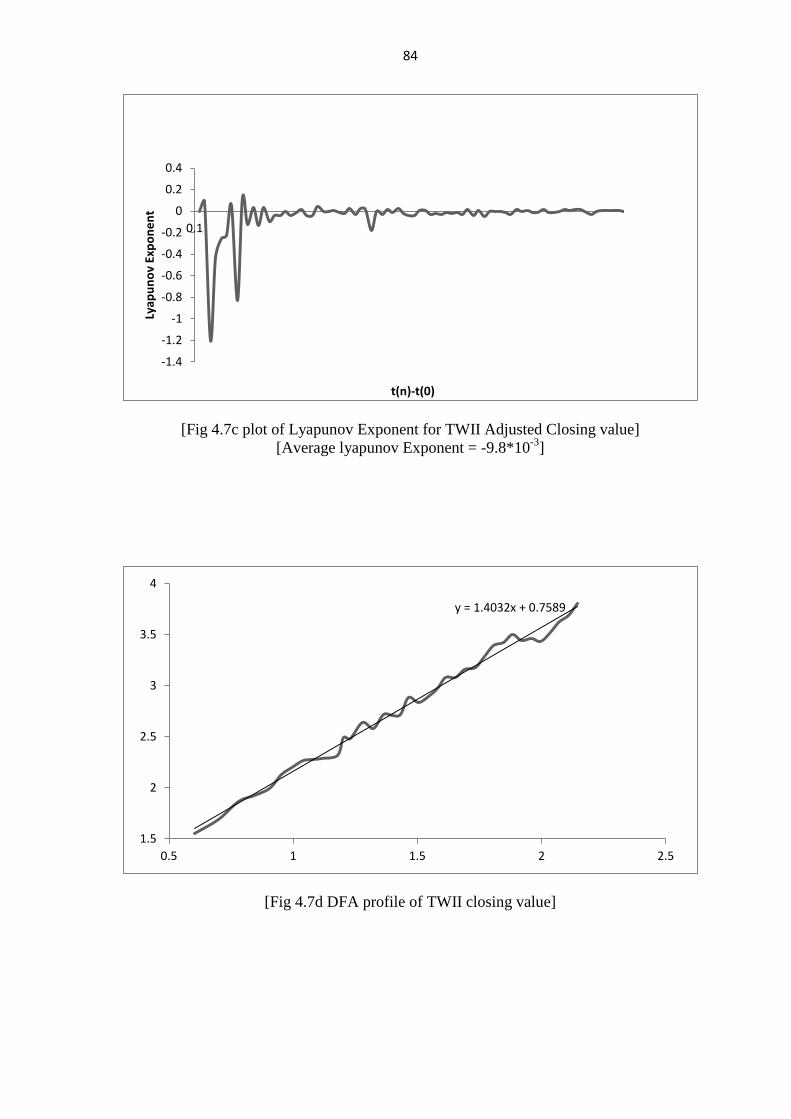
the Plot of TWII Adjusted Closing value. Fig 4.7c is the plot of Lyapunov

Exponent for TWII Adjusted Closing value. Fig 4.7d shows the DFA profile of

TWII closing value.

Plot between data points X(n) and X(n+1) for TWII(volume) is shown

in fig(4.8a). Date was chosen to be 8th

Dec.2009 to 1st Mar.2012. Plot of TWII

trading volume is shown in fig(4.8b) . Plot of Lyapunov exponent for

TWII(volume) is shown in fig(4.8c). The Average Lyapunov exponent was

found to be -5.9*10-3

. DFA Plot for TWII volume is shown in fig(4.8d). The

scaling Exponent was found to be 1.084.

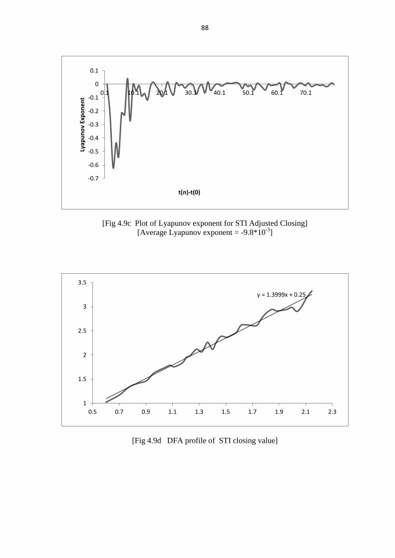
Plot between data points Y(n) and Y(n+1) for STI adjusted Closing

value is shown in fig(4.9a). Date was chosen to be 1st Mar.2012 to 8

th

Jun.2009. Plot of STI adjusted Closing value is shown in fig(4.9b). Plot of

Lyapunov exponent for STI adjusted Closing value is shown in fig(4.9c). DFA

Plot for STI close is shown in fig(4.9d). The scaling Exponent was found to be

1.399.

Plot between data points x(n) and x(n+1) for SEOUL volume is shown


Jun.2009 to 01st Mar 2012. Plot of

SEOUL trading volume is shown in fig(4.10b). Plot of Lyapunov exponent for

SEOUL trading volume is shown in fig(4.10c). The Average Lyapunov

exponent was found to be -1.105*10-3.

DFA Plot for SEOUL volume is shown

in fig (4.10d). The scaling exponent was found to be 0.987.

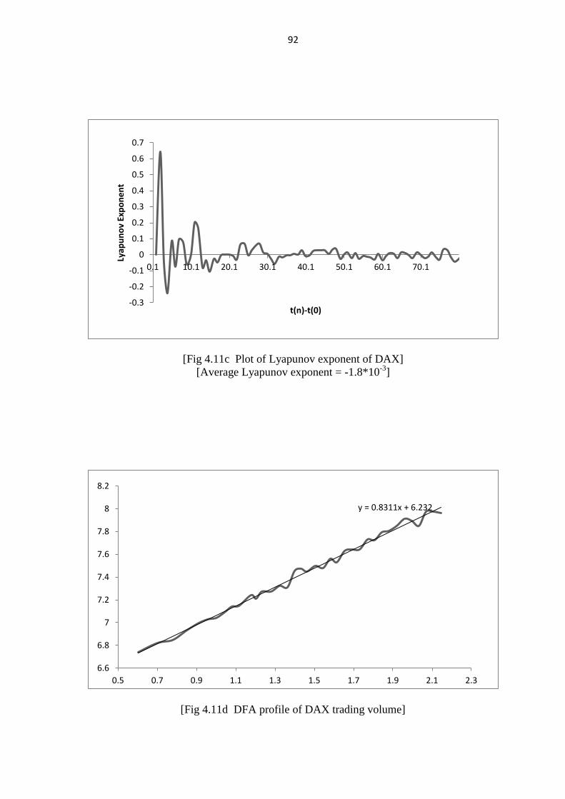
Plot between data points X(n) and X(n+1) for DAX trading volume is

shown in fig(4.11a). Date was chosen to be 9th Apr.2009 to 1

st Apr.2012. Plot

of DAX trading volume is shown in fig(4.11b). Plot of Lyapunov exponent for

DAX (volume) is shown in fig(4.11c). The Average Lyapunov exponent was

found to be -1.8*10-3

. DFA Plot for DAX volume is shown in figure (4.11d).

The scaling exponent was found to be 0.831.

71

Plot between data points Y(n) and Y(n+1) for DAX adjusted Closing

value is shown in fig(4.12a). Date was chosen to be 9th

Apr.2009 to 1st

Apr.2012. Plot of DAX adjusted Closing value is shown in fig(4.12b). Plot of

Lyapunov exponent for DAX adjusted Closing value is shown in fig(4.12c).

The Average Lyapunov exponent was found to be -0.86*10-3

. DFA Plot for

DAX close is shown in fig (4.12d).The scaling exponent was found to be

1.386.

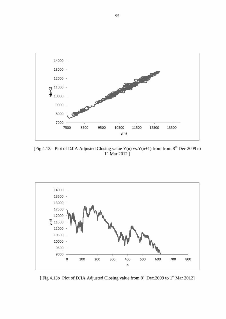
Plot between data points Y(n) and Y(n+1) for DJIA adjusted Closing

value is shown in fig(4.13a) . Date was chosen to be 27th Mar.2009 to 1

st

Mar.2012. Plot of DJIA adjusted Closing value is shown in fig(4.13b. Plot of

Lyapunov exponent for DJIA adjusted Closing value is shown in fig(4.13c).

The average Lyapunov exponent was found to be -9.36*10-3

. DFA Plot for

DJIA closing values is shown in fig(4.13d). The scaling exponent was found to

be 1.420.

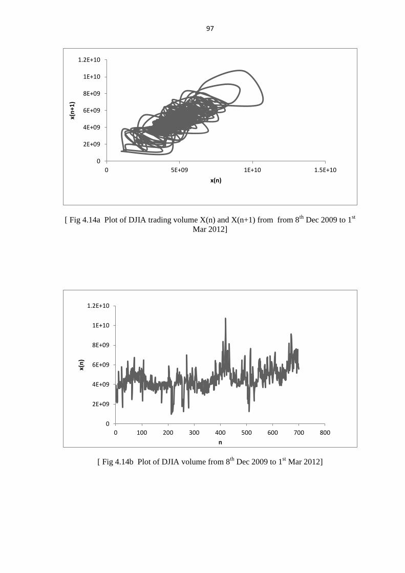
Plot between data points X(n) and X(n+1) for DJIA (volume) is shown


Mar.2009 to 1st Mar.2012. Plot of

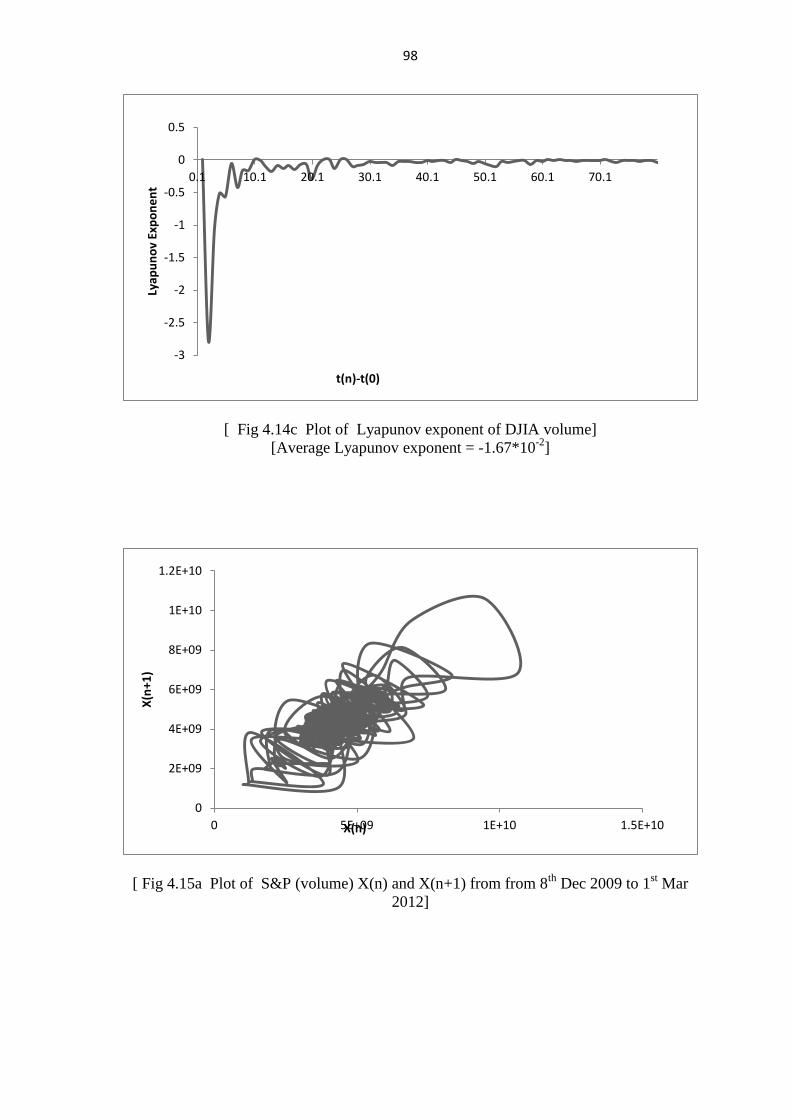
DJIA trading volume is shown in fig(4.14b). Plot of Lyapunov exponent for

DJIA (volume) is shown in fig(4.14c). The average Lyapunov exponent was

found to be -16.7*10-3 .

Plot between data points X(n) and X(n+1) for S&P trading volume is

shown in fig(4.15a). Date was chosen to be 27

th Mar.2009 to 1

st Mar.2012. Plot

of S&P (volume) is shown in fig(4.15b). Plot of Lyapunov exponent for S&P

(volume) is shown in fig(4.15c). The average Lyapunov exponent was found

to be -16.7*10-3 .

Plot between data points Y(n) and Y(n+1) for S&P adjusted Closing

value is shown in fig(4.16a). Date was chosen to be 27th Mar.2009 to 1

st

Mar.2012.Plot of US S&P adjusted Closing value is shown in fig(4.16b). Plot

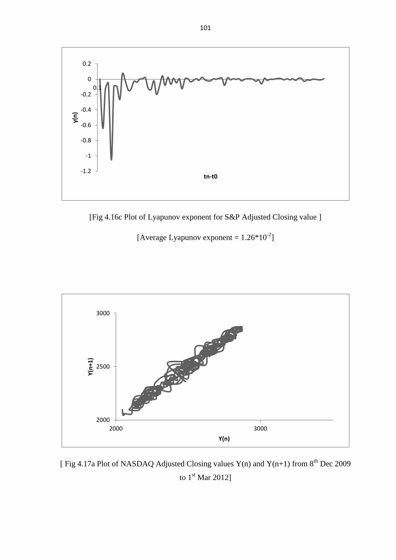
of Lyapunov exponent for S&P adjusted Closing value is shown in fig (4.16c).

The average Lyapunov exponent was found to be -12.6*10-3

.

72

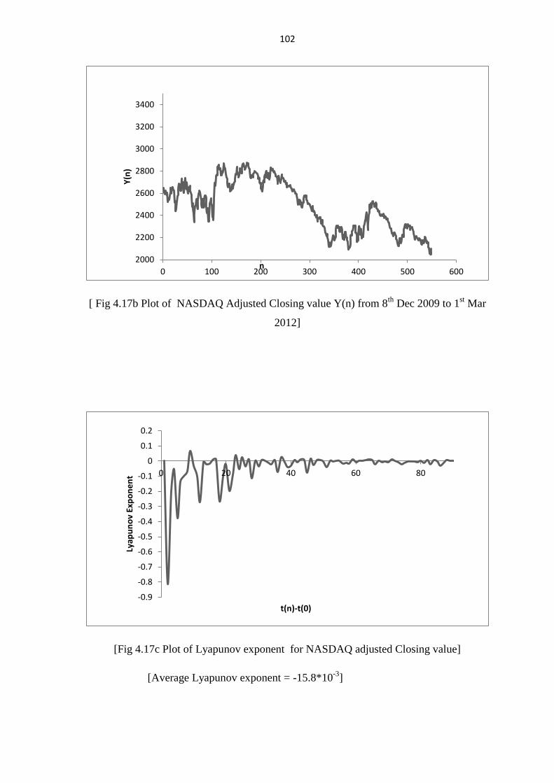
Plot between data points Y(n) and Y(n+1) for NASDAQ adjusted

Closing value is shown in fig(4.17a). Date was chosen to be 29th

Oct.2009 to

1st Mar.2012. Plot of US NASDAQ adjusted Closing value is shown in

fig(4.17b). Plot of Lyapunov exponent for NASDAQ adjusted Closing value is

shown in fig(4.17c). The average Lyapunov exponent was found to be -

15.8*10-3

. DFA Plot for NASDAQ close is shown in fig(4.17d). The scaling

exponent was found to be 1.389.

Plot between data points X(n) and X(n+1) for NASDAQ trading volume

is shown in fig(4.18a). Date was chosen to be 29th

Oct.2009 to 1st Mar.2012 .

Plot of NASDAQ tradingvolume is shown in fig(4.18b). Plot of Lyapunov

exponent for NASDAQ trading volume is shown in fig(4.18c). The average

Lyapunov exponent was found to be -9.6*10-3

. DFA Profile for NASDAQ

volume is shown in fig (4.18d). The scaling exponent was found to be 0.926.

73

[ Fig 4.1a Plot of P/E value of NIFTY { X(0)} from 7th

Jan 1999 to 7th

sep 2001]

[Fig 4.1b Plot of Lyapunov Exponent for P/E value of NIFTY X(0) from 7th

Jan 1999 to

7th

sep 2001. ]

[Average Lyapunov Exponent = - 9.715*10-3

]

0

5

10

15

20

25

30

0 100 200 300 400 500 600 700 800

x( 0

)

t(n)-t(0)

-1.2

-1

-0.8

-0.6

-0.4

-0.2

0

0.2

0 5 10 15 20 25 30 35 40 45 50 55 60 65 70 75 80

Lyap

un

ov

Exp

on

en

t

t(n)-t(0)

74

[Fig 4.1c Plot between x(n+1) and X(n) for P/E value of NIFTY from 7th

Jan 1999 to 7th

sep 2001].

[Fig 4.2a Plot between time and P/E value of NIFTY Y(0) from 17th

Sep 2001 to 1st Jan

2004 ]

11

16

21

26

31

12 24

x(n

+1)

x(n)

0

5

10

15

20

25

0 200 400 600 800

y(0

)

t(n)-t(0)

75

[ Fig 4.2b Plot of Lyapunov Exponent for P/E value of NIFTY Y(0) from 17th

Sep 2001

to 1st Jan 2004 ]

[Average Lyapunov Exponent = -1.25*10-3

]

[ Fig 4.2c Plot between Y(n+1) and Y(n) P/E value of NIFTY from 17th

Sep 2001 to 1st Jan

2004]

-0.2

-0.1

0

0.1

0.2

0.3

0.4

0.5

0 40 80

Lyap

un

ov

Exp

on

en

t

t(n)-t(0)

10

15

20

25

11 16 21 26

y(n

+1)

y(n)

76

[Fig 4.3a Plot of P/E value of NIFTY Z(0) from 1st Jan 1999 to 15

th Dec 2011 ]

[ Fig 4.3b Plot of Lyapunov exponent for P/E value of NIFTY Z(0) from 1st Jan 1999 to

15th

Dec 2011].

[Average lyapunov Exponent = -6.79*10-3

]

0

5

10

15

20

25

0 100 200 300 400 500 600 700 800

Z(0

)

t(n)-t(0)

-0.9

-0.8

-0.7

-0.6

-0.5

-0.4

-0.3

-0.2

-0.1

0

0.1

0.2

0 40 80

Lyap

un

ov

Exp

on

en

t

t(n)-t(0)

77

[Fig 4.3c Plot between Z(n+1) and Z(n) P/E value of NIFTY 1st Jan 1999 to 15

th Dec 2011]

[Fig 4.4a Combined Plot of x(0),y(0),z(0). In graph Blue line indicate the variation of data

point X(0) , Red line indicate the variation of data point Y(0) ,Green line indicate the

variation of data point Z(0)]

Average Lyapunov exponent for x(0) = - 9.715*10-3

.

Average Lyapunov exponent for y(0) = -1.25*10-3

Average Lyapunov exponent for z(0) = -6.79*10-3

.

11

13

15

17

19

21

23

25

11 13 15 17 19 21 23 25

z(n

+1)

z(n)

0

5

10

15

20

25

30

0 200 400 600 800

x(0

),y(

0),

z(0

)

t(n)-t(0)

x0

y0

Z0

78

[ Fig 4.4b Plot between time and Lyapunov exponent for X(0) Y(0),Z(0) 7th

Jan 1999 to 9th

Feb 2007].

[Average Lyapunov exponent for X(0) = - 9.715*10-3

.

Average Lyapunov exponent for Y(0) = -1.25*10-3

Average Lyapunov exponent for Z(0) = -6.79*10-3

]

-1.2

-1

-0.8

-0.6

-0.4

-0.2

0

0.2

0.4

0.6

0 40 80

Lyap

un

ov

Exp

on

en

t

t(n)-t(0)

lyp for x0

lyp for y0

lyp for z0

79

[Fig 4.5a Plot between X(n) and X(n+1) for NIKKEI (volume) 21st Jul 2009 to30

th Dec

2011 ]

[Fig 4.5b Plot of NIKKEI (volume) from 21st Jul 2009 to 30

th Dec 2011 ].

-50000

0

50000

100000

150000

200000

250000

300000

350000

400000

450000

-100000 0 100000 200000 300000 400000 500000

X(n

+1)

X(n)

-50000

0

50000

100000

150000

200000

250000

300000

350000

400000

450000

0 100 200 300 400 500 600 700

X(n

)

n

80

[ Fig 4.5c Plot of Lyapunov Exponent for Nikkei (volume) from 21st Jul 2009 to 30

th Dec

2011]


]

[Fig 4.5d DFA profile of NIKKEI volume]

y = 0.9623x + 3.502

4

4.2

4.4

4.6

4.8

5

5.2

5.4

5.6

5.8

0.5 1 1.5 2 2.5

-0.4

-0.3

-0.2

-0.1

0

0.1

0.2

0.3

0.4

0

Lyap

un

ov

Exp

on

en

t

t(n)-t(0)

81

[Fig 4.6a Plot of NIKKEI Ajdusted closing value Y(n) and Y(n+1)]

[Fig 4.6b Plot of NIKKEI Adjusted Closing value Y(n) during 30th

21st Jul 2009 to 30

th Dec

2012 ]

8000

8500

9000

9500

10000

10500

11000

11500

12000

8000 9000 10000 11000 12000

Ad

just

ed

clo

se Y

(n+1

)

Adjusted close Y(n)

8000

10000

0 100 200 300 400 500 600 700

Y(n

)

n

82

[Fig 4.6c Plot of Lyapunov exponent for NIKKEI Adjusted Closing value ]

[Average Lyapunov exponent = -.0104*10-3

]

[Fig 4.6d DFA profile of NIKKEI closing value]

-0.5

-0.4

-0.3

-0.2

-0.1

0

0.1

0.2

0.1

lyap

un

ov

Exp

on

en

t

t(n)-t(0)

y = 1.3855x + 0.9248

2

2.5

3

3.5

4

4.5

0.5 1 1.5 2 2.5

83

[ Fig 4.7a Plot of TWII Adjusted Closing value data point Y(n) and Y(n+1) during the

period from to 8th

Dec 2009 1st Mar 2012] .

[Fig 4.7b Plot of TWII Adjusted Closing value Y(n) from 12th

Aug.2009 to 1st Mar.2012].

6000

6500

7000

7500

8000

8500

9000

9500

10000

6500 7000 7500 8000 8500 9000 9500 10000

y(n

+1)

6000

6500

7000

7500

8000

8500

9000

9500

10000

0 100 200 300 400 500 600 700

y(n

)

n

84

[Fig 4.7c plot of Lyapunov Exponent for TWII Adjusted Closing value]


]

[Fig 4.7d DFA profile of TWII closing value]

-1.4

-1.2

-1

-0.8

-0.6

-0.4

-0.2

0

0.2

0.4

0.1

Lyap

un

ov

Exp

on

en

t

t(n)-t(0)

y = 1.4032x + 0.7589

1.5

2

2.5

3

3.5

4

0.5 1 1.5 2 2.5

85

[ Fig 4.8a Plot between TWII(volume) data point X(n) and X(n+1) from 8th

Dec 2009 to 1st

Mar 2012]

[Fig 4.8b Plot of TWII trading volume from from 8th

Dec 2009 to 1st Mar 2012].

0

1000000

2000000

3000000

4000000

5000000

6000000

7000000

8000000

0 2000000 4000000 6000000 8000000

x(n

+1)

x(n)

0

1000000

2000000

3000000

4000000

5000000

6000000

7000000

8000000

0 100 200 300 400 500 600 700

x(n

)

n

86

[Fig 4.8c Plot of Lyapunov exponent of TWII trading volume]

[Average Lyapunov exponent = -5.8*10-3

]

[Fig 4.8d DFA profile of TWII volume]

-0.4

-0.3

-0.2

-0.1

0

0.1

0.2

0.1 20.1 40.1 60.1

Lyap

un

ov

Exp

on

en

t

t(n)-t(0)

y = 1.0842x + 4.6424

5

5.5

6

6.5

7

7.5

0.5 0.7 0.9 1.1 1.3 1.5 1.7 1.9 2.1 2.3

87

[Fig 4.9a Plot between STI Adjusted Closing value Y(n) and Y(n+1) from 8th

Dec 2009 to

1st Mar 2012].

[Fig 4.9b Plot of STI Adjusted Closing value from 8th

Dec 2009 to 1st Mar 2012].

2400

2600

2800

3000

3200

3400

2500 2700 2900 3100 3300 3500

y(n

+1)

STI data points y(n)

2500

3000

0 100 200 300 400 500 600 700

Y(n

)

n

88

[Fig 4.9c Plot of Lyapunov exponent for STI Adjusted Closing]


]

[Fig 4.9d DFA profile of STI closing value]

-0.7

-0.6

-0.5

-0.4

-0.3

-0.2

-0.1

0

0.1

0.1 10.1 20.1 30.1 40.1 50.1 60.1 70.1

Lyap

un

ov

Exp

on

en

t

t(n)-t(0)

y = 1.3999x + 0.25

1

1.5

2

2.5

3

3.5

0.5 0.7 0.9 1.1 1.3 1.5 1.7 1.9 2.1 2.3

89

[ Fig 4.10a Plot of SEOUL closing values X(n) and X(n+1) from 8th

Dec 2009 to 1st Mar

2012]

[Fig 4.10b Plot of SEOUL volume from 8th

Dec 2009 to 1st Mar 2012]

0

100000

200000

300000

400000

500000

600000

700000

800000

0 100000 200000 300000 400000 500000 600000 700000 800000

X(n

+1)

X(n)

0

100000

200000

300000

400000

500000

600000

700000

800000

0 100 200 300 400 500 600 700

X(n

)

n

Volume x(n)

90

[Fig 4.10c Plot of Lyapunov exponent for SEOUL trading volume]


]

[Fig 4.10d DFA Profile of SEOUL trading volume]

-1

-0.8

-0.6

-0.4

-0.2

0

0.2

0.1

Lyap

un

ov

Exp

on

en

t

t(n)-t(0)

y = 0.9871x + 3.7506

4

4.2

4.4

4.6

4.8

5

5.2

5.4

5.6

5.8

6

0.5 0.7 0.9 1.1 1.3 1.5 1.7 1.9 2.1 2.3

91

[Fig 4.11a Plot between DAX (volume) data point X(n) and X(n+1) from 8th

Dec 2009 to

1st Mar 2012]

[Fig 4.11b Plot of DAX trading volume 8th


0

20000000

40000000

60000000

80000000

100000000

120000000

140000000

0 50000000 100000000 150000000

x(n

+1)

x(n)

0

20000000

40000000

60000000

80000000

100000000

120000000

140000000

0 100 200 300 400 500 600 700

x(n

)

n

Volume x(n)

92

[Fig 4.11c Plot of Lyapunov exponent of DAX]


]

[Fig 4.11d DFA profile of DAX trading volume]

-0.3

-0.2

-0.1

0

0.1

0.2

0.3

0.4

0.5

0.6

0.7

0.1 10.1 20.1 30.1 40.1 50.1 60.1 70.1

Lyap

un

ov

Exp

on

en

t

t(n)-t(0)

y = 0.8311x + 6.232

6.6

6.8

7

7.2

7.4

7.6

7.8

8

8.2

0.5 0.7 0.9 1.1 1.3 1.5 1.7 1.9 2.1 2.3

93

[Fig 4.12a Plot of DAX Adjusted Closing value Y(n) and Y(n+1) from 8th

Dec.2009 to 1st

Mar.2012]

[Fig 4.12b Plot OF DAX adjusted Closing value from 8th


5000

5500

6000

6500

7000

7500

8000

5000 5500 6000 6500 7000 7500 8000

y(n

+1)

y(n)

5000

5500

6000

6500

7000

7500

8000

0 100 200 300 400 500 600 700

y(n

)

n

94

[ Fig 4.12c Plot of Lyapunov exponent for DAX Adjusted Closing value]


]

[Fig 4.12d DFA profile of DAX closing values]

-0.4

-0.2

0

0.2

0.4

0.6

0.8

1

0.1 10.1 20.1 30.1 40.1 50.1 60.1 70.1

Lyap

un

ov

Exp

on

en

t

t(n)-t(0)

y = 1.3862x + 0.7638

1.5

2

2.5

3

3.5

4

0.5 0.7 0.9 1.1 1.3 1.5 1.7 1.9 2.1 2.3

95

[Fig 4.13a Plot of DJIA Adjusted Closing value Y(n) vs.Y(n+1) from from 8th

Dec 2009 to

1st Mar 2012 ]

[ Fig 4.13b Plot of DJIA Adjusted Closing value from 8th

Dec.2009 to 1st Mar 2012]

7000

8000

9000

10000

11000

12000

13000

14000

7500 8500 9500 10500 11500 12500 13500

y(n

+1)

y(n)

9000

9500

10000

10500

11000

11500

12000

12500

13000

13500

14000

0 100 200 300 400 500 600 700 800

y(n

)

n

96

[Fig 4.13c Lyapunov exponent of DJIA]


]

[Fig 4.13d DFA profile of DJIA]

-1

-0.8

-0.6

-0.4

-0.2

0

0.2

0.1

Lyap

un

ov

Exp

on

en

t

t(n)-t(0)

y = 1.4205x + 0.8294

1.5

2

2.5

3

3.5

4

4.5

0.5 1 1.5 2 2.5

97

[ Fig 4.14a Plot of DJIA trading volume X(n) and X(n+1) from from 8th

Dec 2009 to 1st

Mar 2012]

[ Fig 4.14b Plot of DJIA volume from 8th


0

2E+09

4E+09

6E+09

8E+09

1E+10

1.2E+10

0 5E+09 1E+10 1.5E+10

x(n

+1)

x(n)

0

2E+09

4E+09

6E+09

8E+09

1E+10

1.2E+10

0 100 200 300 400 500 600 700 800

x(n

)

n

98

[ Fig 4.14c Plot of Lyapunov exponent of DJIA volume]


]

[ Fig 4.15a Plot of S&P (volume) X(n) and X(n+1) from from 8th

Dec 2009 to 1st Mar

2012]

-3

-2.5

-2

-1.5

-1

-0.5

0

0.5

0.1 10.1 20.1 30.1 40.1 50.1 60.1 70.1

Lyap

un

ov

Exp

on

en

t

t(n)-t(0)

0

2E+09

4E+09

6E+09

8E+09

1E+10

1.2E+10

0 5E+09 1E+10 1.5E+10

X(n

+1)

X(n)

99

[ Fig 4.15b Plot of S&P (volume) from 8th

Dec 2009 to 1st Mar 2012].

[ Fig 4.15c Plot of Lyapunov exponent of S&P volume]


]

0

2E+09

4E+09

6E+09

8E+09

1E+10

1.2E+10

0 100 200 300 400 500

X(n

)

n

-3

-2.5

-2

-1.5

-1

-0.5

0

0.5

0.1

Lyap

un

ov

Exp

on

en

t

t(n)-t(0)

100

Fig 4.16aPlot of S&P Adjusted Closing values Y(n) vs. Y(n+1) from 8th

Dec 2009 to 1st

Mar 2012]

[ Fig 4.16b Plot of S&P Adjusted Closing value from 8th


1000

1200

1400

1000 1050 1100 1150 1200 1250 1300 1350 1400 1450 1500

y(n

+1)

y(n)

1000

1200

1400

0 100 200 300 400 500

y(n

)

n

101

[Fig 4.16c Plot of Lyapunov exponent for S&P Adjusted Closing value ]

[Average Lyapunov exponent = 1.26*10-2

]

[ Fig 4.17a Plot of NASDAQ Adjusted Closing values Y(n) and Y(n+1) from 8th

Dec 2009

to 1st Mar 2012]

-1.2

-1

-0.8

-0.6

-0.4

-0.2

0

0.2

0.1

y(n

)

tn-t0

2000

2500

3000

2000 3000

Y(n

+1)

Y(n)

102

[ Fig 4.17b Plot of NASDAQ Adjusted Closing value Y(n) from 8th

Dec 2009 to 1st Mar

2012]

[Fig 4.17c Plot of Lyapunov exponent for NASDAQ adjusted Closing value]


]

2000

2200

2400

2600

2800

3000

3200

3400

0 100 200 300 400 500 600

Y(n

)

n

-0.9

-0.8

-0.7

-0.6

-0.5

-0.4

-0.3

-0.2

-0.1

0

0.1

0.2

0 20 40 60 80

Lyap

un

ov

Exp

on

en

t

t(n)-t(0)

103

[Fig 4.17d DFA profile for NASDAQ closing values]

[ Fig 4.18a Plot of NASDAQ volume data points X(n) vs. X(n+1) from from 8th

Dec 2009

to 1st Mar 2012].

y = 1.3893x + 0.3132

1

1.5

2

2.5

3

3.5

0.5 0.7 0.9 1.1 1.3 1.5 1.7 1.9 2.1 2.3

0

500000000

1E+09

1.5E+09

2E+09

2.5E+09

3E+09

3.5E+09

4E+09

4.5E+09

5E+09

0 2E+09 4E+09 6E+09

X(n

+1)

X(n)

104

[ Fig 4.18b Plot of NASDAQ volume X(n) from 8th


[ Fig 4.18c Plot of Lyapunov exponent of NASDAQ volume ]


]

0

500000000

1E+09

1.5E+09

2E+09

2.5E+09

3E+09

3.5E+09

4E+09

4.5E+09

5E+09

0 100 200 300 400 500 600

X(n

)

n

-1.4

-1.2

-1

-0.8

-0.6

-0.4

-0.2

0

0.2

0.1

Lyap

un

ov

Exp

on

en

t

t(n)-t(0)

105

[Fig 4.18d DFA profile for NASDAQ volume]

y = 0.9265x + 7.5732

8

8.2

8.4

8.6

8.8

9

9.2

9.4

9.6

9.8

0.5 0.7 0.9 1.1 1.3 1.5 1.7 1.9 2.1 2.3

106

4.3 Discussion

Time series data for different indices were studied using Lyapunov

exponent method. The outcome of the study is as follows : The Lyapunov

eExponent for Values of NIKKI trading volume is found to be positive for the

data studied, confirming the presence of chaos for the period under study. It

shows the divergent behavior of trajectory whereas the Lyapunov exponent for

NIKKI Adjusted Closing value is negative for the data studied confirming the

absence of chaos for the period under study. It shows the convergent behavior

of trajectory. The Lyapunov exponent for Values of TWII volume and

Adjusted Closing value is found to be negative for the data studied confirming

the absence of chaos for the period under study showing the convergent

behavior of trajectory. The Lyapunov exponent for STI adjusted Closing value

is found to be negative for the data studied confirming the absence of chaos for

the period under study. It shows the convergent behavior of trajectory. The

Lyapunov exponent for SEOUL trading volume is found to be negative for the

data studied confirming the absence of chaos for the period under study. It

shows the convergent behavior of trajectory. The Lyapunov exponent DAX

volume and adjusted closing values is found to be negative for the data studied

confirming the absence of chaos for the period under study. It shows the

convergent behavior of trajectory. The Lyapunov exponent for DJIA Volume

and Adjusted Closing value is found to be negative for the data studied


convergent behavior of trajectory. The Lyapunov exponent for S&P Volume

and Adjusted Closing value is found to be negative for the data studied


convergent behavior of trajectory. The Lyapunov exponent for NASDAQ

Volume and Adjusted Closing value is found to be negative for the data

studied confirming the absence of chaos for the period under study. It shows

the convergent behavior of trajectory. The Lyapunov exponent for P/E value of

NIFTY is found to be negative for the data studied confirming the absence of

chaos for the period under study. It shows the convergent behavior of

trajectory.

107

4.4 References

[1]. Holger Kantz and Thomas Schriber, Nonlineae time series analysis,

Cambridge university press(2005)

[2]. T.Rosentein, J.J.Collins, C.J. De Luca, A practical method for calculating

largest lyapunov exponent from small data sets., physica D, 65, 73,82

(1993)

[3]. H. D. I. Abarbanel, R. Brown, and J. B. Kadtke, Prediction in chaotic

nonlinear systems: methods for time series with broadband Fourier spectra,

Phys. Rev. A 41, 1782, (1990).

[4]. N. B. Abraham, A. M. Albano, B. Das, G. De Guzman, S. Yong, R. S.

Gioggia, G. P.Puccioni, and J. R. Tredicce, Calculating the dimension of

attractors from small data sets, Phys. Lett. A 114,217(1986).

[5]. A. M. Albano, J. Muench, C. Schwartz, A. I. Mees, and P. E. Rapp,

Singular-value decomposition and the Grassberger-Procaccia algorithm,

Phys. Rev. A 38, 3017 (1988).

[6]. A. M. Albano, A. Passamante, and M. E. Farrell, Using higher-order

correlations to define an embedding window, Physica D 54, 85 (1991).

[7]. G. Benettin, C. Froeschle, and J. P. Scheidecker, Kolmogorov entropy of a

dynamical system with increasing number of degrees of freedom, Phys.

Rev. A 19, 2454 (1979).

[8]. G. Benettin, L. Galgani, and J.-M. Strelcyn, Kolmogorov entropy and

numerical experiments, Phys. Rev. A 14, 2338 (1976).

[9]. K. Briggs, An improved method for estimating Liapunov exponents of

chaotic time series, Phys. Lett. A 151, 27 (1990).

[10]. D. S. Broomhead, and G. P. King, Extracting qualitative dynamics from

experimental data, Physica D 20, 217 (1986).

[11]. R. Brown, P. Bryant, and H. D. I. Abarbanel, Computing the Lyapunov

spectrum of a dynamical system from observed time series, Phys. Rev. A

43, 2787 (1991).

[12]. M. Casdagli, Nonlinear prediction of chaotic time series, Physica D 35 ,

335 (1989).

[13]. P. Chen, Empirical and theoretical evidence of economic chaos, Sys. Dyn.

Rev. 4, 81 (1988)

108

[14]. J. Deppisch, H.-U. Bauer, and T. Geisel, Hierarchical training of neural

networks and prediction of chaotic time series, Phys. Lett. A 158, 57

(1991).

[15]. J.-P. Eckmann, S. O. Kamphorst, D. Ruelle, and S. Ciliberto, Liapunov

exponents from time series, Phys. Rev. A 34, 4971 (1986).

[16]. J.-P. Eckmann, and D. Ruelle, Fundamental limitations for estimating

dimensions and Lyapunov exponents in dynamical systems, Physica D 56 ,

185 (1992).

[17]. J.-P. Eckmann, and D. Ruelle, Ergodic theory of chaos and strange

attractors, Rev. Mod. Phys. 57, 617 (1985).

[18]. S. Ellner, A. R. Gallant, D. McCaffrey, and D. Nychka, Convergence rates

and data requirements for Jacobian-based estimates of Lyapunov

exponents from data, Phys. Lett. A 153, 357 (1991).

[19]. J. D. Farmer, and J. J. Sidorowich, Predicting chaotic time series, Phys.

Rev. Lett. 59, 845 (1987).

[20]. G. W. Frank, T. Lookman, M. A. H. Nerenberg, C. Essex, J. Lemieux, and

W. Blume, Chaotic time series analysis of epileptic seizures, Physica D 46,

427 (1990).

[21]. A. M. Fraser, and H. L. Swinney, Independent coordinates for strange

attractors from mutual information, Phys. Rev. A 33, 1134 (1986).

[22]. P. Grassberger, and I. Procaccia, Characterization of strange attractors,

Phys. Rev. Lett. 50, 346 (1983).

[23]. P. Grassberger, and I. Procaccia, Estimation of the Kolmogorov entropy

from a chaotic signal, Phys. Rev. A 28, 2591 (1983).

[24]. M. Hénon, A two-dimensional mapping with a strange attractor, Comm.

Math. Phys. 50, 69 (1976).

[25]. W. Liebert, and H. G. Schuster, Proper choice of the time delay for the

analysis of chaotic time series, Phys. Lett. A 142, 107. 21 (1989)

[26]. E. N. Lorenz, Deterministic nonperiodic flow, J. Atmos. Sci. 20, 130

(1963).

[27]. M. C. Mackey, and L. Glass, Oscillation and chaos in physiological control

systems, Science 197, 287 (1977).

109

[28]. V. I. Oseledec, A multiplicative ergodic theorem. Lyapunov characteristic

numbers for dynamical systems, Trans. Moscow Math. Soc. 19, 197

(1968).

[29]. N. H. Packard, J. P. Crutchfield, J. D. Farmer, and R. S. Shaw, Geometry

from a time series, Phys. Rev. Lett. 45, 712 (1980).

[30]. J. B. Ramsey, and H.-J. Yuan, The statistical properties of dimension

calculations using small data sets, Nonlinearity 3, 155 (1990).

[31]. F. Rauf, and H. M. Ahmed, Calculation of Lyapunov exponents through

`nonlinear adaptive filters, Proceedings IEEE International Symposium on

Circuits and Systems, Singapore (1991).

[32]. O. E. Rössler, An equation for hyperchaos, Phys. Lett. A 71, 155 (1979).

[33]. O. E. Rössler, An equation for continuous chaos, Phys.Lett. A, 397

57(1976).

[34]. M. Sano, and Y. Sawada, Measurement of the Lyapunov spectrum from a

chaotic time series, Phys. Rev. Lett. 55, 1082 (1985).

[35]. S. Sato, M. Sano, and Y. Sawada, Practical methods of measuring the

generalized dimension and the largest Lyapunov exponent in high

dimensional chaotic systems, Prog. Theor. Phys. 77, 1 (1987).

[36]. I. Shimada, and T. Nagashima, A numerical approach to ergodic problem

of dissipative dynamical systems, Prog. Theor. Phys. 61, 1605 (1979).

[37]. R. Stoop, and J. Parisi, Calculation of Lyapunov exponents avoiding

spurious elements,Physica D 50, 89.22 (1991)

[38]. G. Sugihara, and R. M. May, Nonlinear forecasting as a way of

distinguishing chaos from measurement error in time series, Nature 344 ,

734 (1990).

[39]. F. Takens, Detecting strange attractors in turbulence, Lect. Notes in Math.

898, 366 (1981).

[40]. D. J. Wales, Calculating the rate loss of information from chaotic time

series by forecasting, Nature 350, 485 (1991).

[41]. A. Wolf, J. B. Swift, H. L. Swinney, and J. A. Vastano, Determining

Lyapunov exponents from a time series, Physica D 16 (1985) 285.

[42]. J. Wright, Method for calculating a Lyapunov exponent, Phys. Rev. A 29,

2924 (1984).

CHAPTER 4 LYAPUNOV EXPONENT - Shodhgangashodhganga.inflibnet.ac.in/bitstream/10603/7179/12/12_chapter 4.pdf · 68 gives the average exponential rate of divergence or convergence of

Documents