Chapter 4 Digital Transmission. 4.1 Line Coding Some Characteristics Line Coding Schemes Some Other Schemes.

Chapter 4

DigitalTransmission

4.1 Line Coding

Some Characteristics

Line Coding Schemes

Some Other Schemes

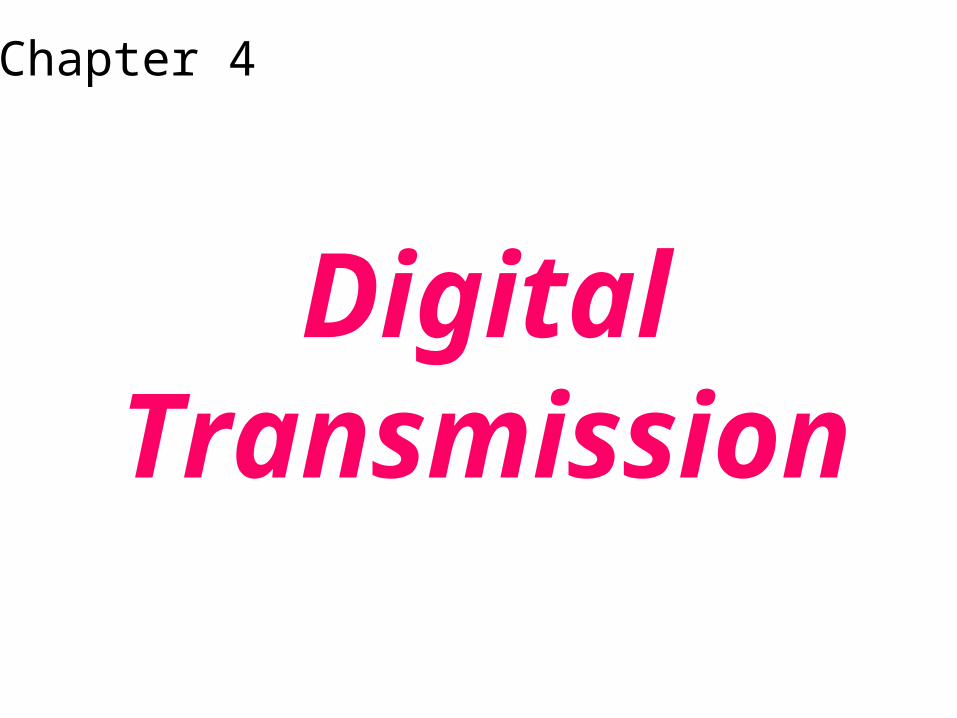
Figure 4.1 Line coding

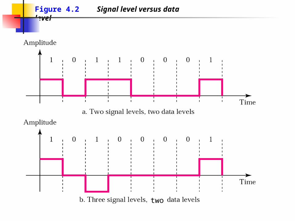
Figure 4.2 Signal level versus data level

two

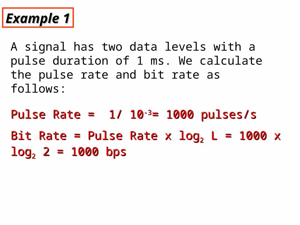
Example 1Example 1

A signal has two data levels with a pulse duration of 1 ms. We calculate the pulse rate and bit rate as follows:

Pulse Rate = 1/ 10Pulse Rate = 1/ 10-3-3= 1000 pulses/s= 1000 pulses/s

Bit Rate = Pulse Rate x logBit Rate = Pulse Rate x log22 L = 1000 x log L = 1000 x log22 2 = 1000 bps 2 = 1000 bps

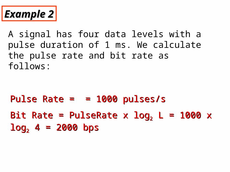
Example 2Example 2

A signal has four data levels with a pulse duration of 1 ms. We calculate the pulse rate and bit rate as follows:

Pulse Rate = = 1000 pulses/sPulse Rate = = 1000 pulses/s

Bit Rate = PulseRate x logBit Rate = PulseRate x log22 L = 1000 x log L = 1000 x log22 4 = 2000 bps 4 = 2000 bps

Figure 4.4 Lack of synchronization

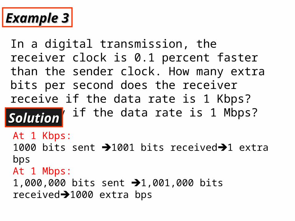
Example 3Example 3

In a digital transmission, the receiver clock is 0.1 percent faster than the sender clock. How many extra bits per second does the receiver receive if the data rate is 1 Kbps? How many if the data rate is 1 Mbps?

SolutionSolutionAt 1 Kbps:1000 bits sent 1001 bits received1 extra bpsAt 1 Mbps: 1,000,000 bits sent 1,001,000 bits received1000 extra bps

Figure 4.5 Line coding schemes

Unipolar encoding uses only one voltage level.

Note:Note:

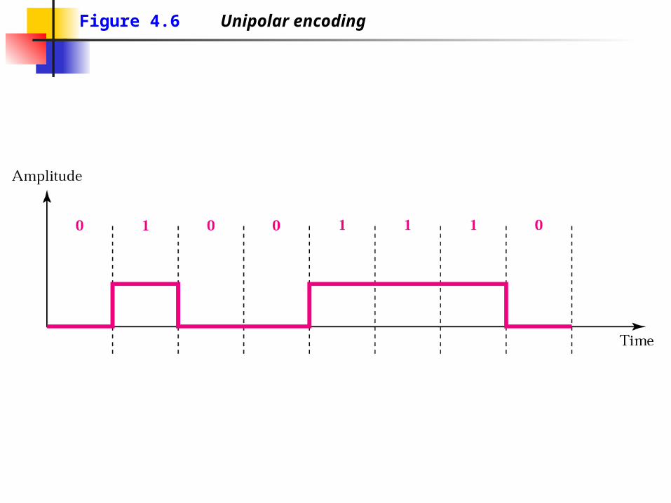
Figure 4.6 Unipolar encoding

Polar encoding uses two voltage levels Polar encoding uses two voltage levels (positive and negative).(positive and negative).

Note:Note:

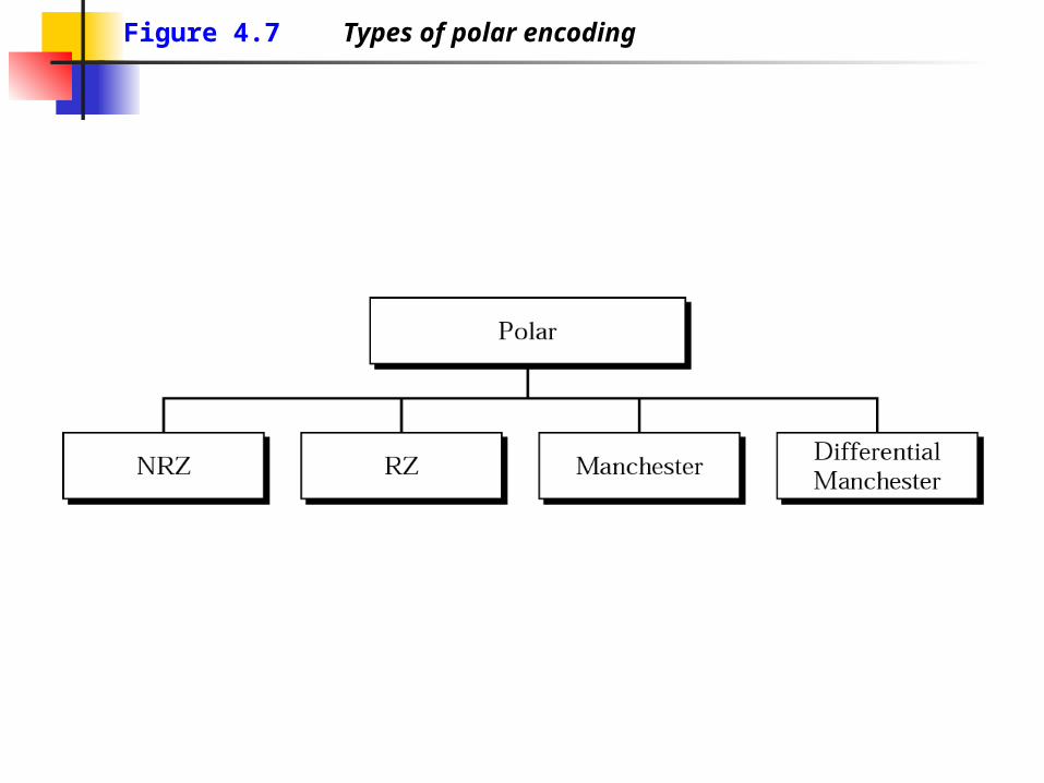
Figure 4.7 Types of polar encoding

In NRZ-L the level of the signal is In NRZ-L the level of the signal is dependent upon the state of the bit.dependent upon the state of the bit.

Note:Note:

In NRZ-I the signal is inverted if a 1 is In NRZ-I the signal is inverted if a 1 is encountered.encountered.

Note:Note:

Figure 4.8 NRZ-L and NRZ-I encoding

Figure 4.9 RZ encoding

A good encoded digital signal must A good encoded digital signal must contain a provision for contain a provision for

synchronization.synchronization.

Note:Note:

Figure 4.10 Manchester encoding

In Manchester encoding, the In Manchester encoding, the transition at the middle of the bit is transition at the middle of the bit is

used for both synchronization and bit used for both synchronization and bit representation.representation.

Note:Note:

Figure 4.11 Differential Manchester encoding

In differential Manchester encoding, In differential Manchester encoding, the transition at the middle of the bit is the transition at the middle of the bit is

used only for synchronization. used only for synchronization. The bit representation is defined by the The bit representation is defined by the

inversion or noninversion at the inversion or noninversion at the beginning of the bit.beginning of the bit.

Note:Note:

In bipolar encoding, we use three In bipolar encoding, we use three levels: positive, zero, levels: positive, zero,

and negative.and negative.

Note:Note:

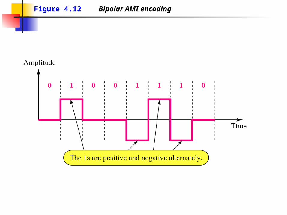
Figure 4.12 Bipolar AMI encoding

B8ZS

Bipolar With 8 Zeros Substitution Based on bipolar-AMI If octet of all zeros and last voltage pulse

preceding was positive encode as 000+-0-+ If octet of all zeros and last voltage pulse

preceding was negative encode as 000-+0+-

Causes two violations of AMI code Receiver detects and interprets as octet of

all zeros

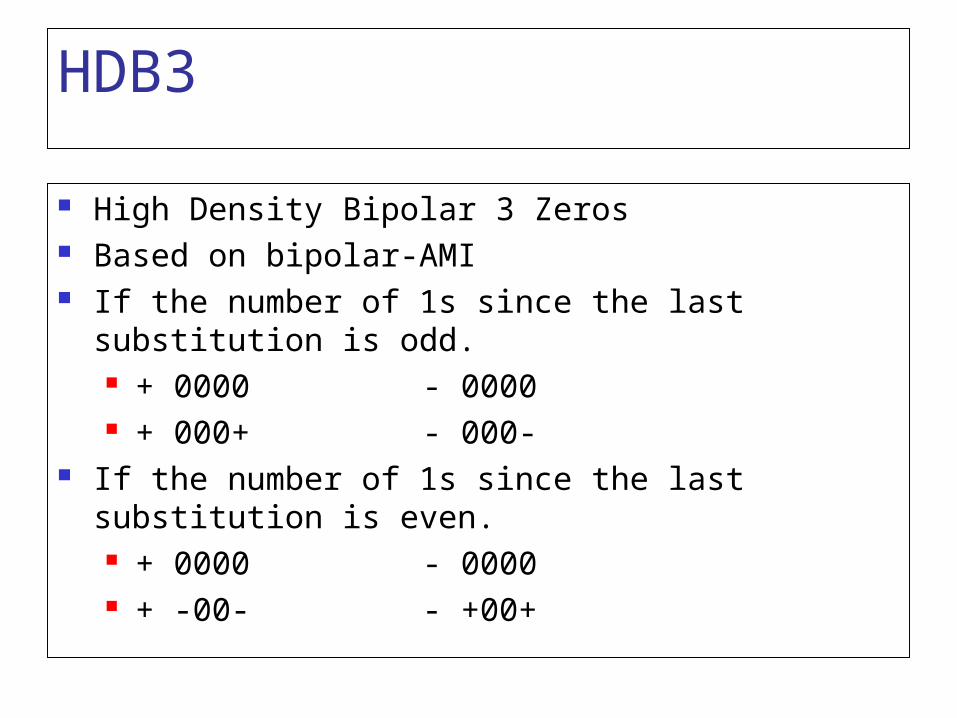
HDB3

High Density Bipolar 3 Zeros Based on bipolar-AMI If the number of 1s since the last substitution is

odd. + 0000 - 0000 + 000+ - 000-

If the number of 1s since the last substitution is even. + 0000 - 0000 + -00- - +00+

B8ZS and HDB3

Figure 4.13 2B1Q

Figure 4.14 MLT-3 signal

4.2 Block Coding

Steps in Transformation

Some Common Block Codes

Figure 4.15 Block coding

Figure 4.16 Substitution in block coding

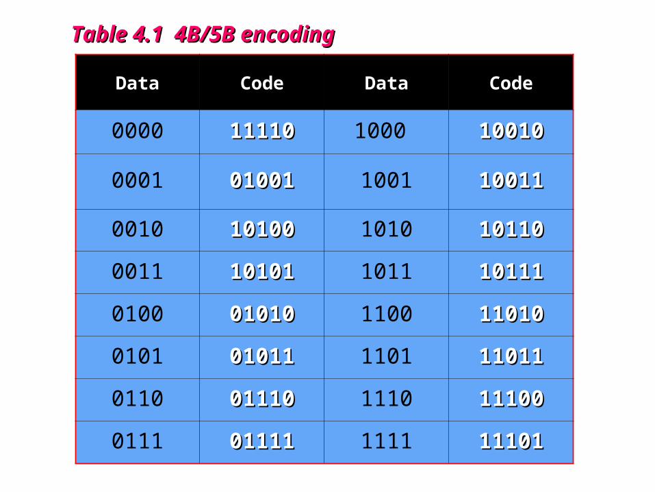
Table 4.1 4B/5B encodingTable 4.1 4B/5B encoding

Data Code Data Code

0000 1111011110 1000 1001010010

0001 0100101001 1001 1001110011

0010 1010010100 1010 1011010110

0011 1010110101 1011 1011110111

0100 0101001010 1100 1101011010

0101 0101101011 1101 1101111011

0110 0111001110 1110 1110011100

0111 0111101111 1111 1110111101

Figure 4.17 Example of 8B/6T encoding

4.3 Sampling4.3 Sampling

Pulse Amplitude ModulationPulse Code ModulationSampling Rate: Nyquist TheoremHow Many Bits per Sample?Bit Rate

Figure 4.18 PAM

Figure 4.19 Quantized PAM signal

Figure 4.20 Quantizing by using sign and magnitude

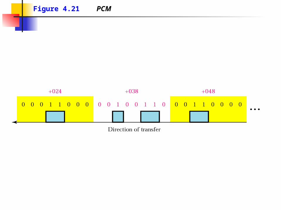
Figure 4.21 PCM

Figure 4.22 From analog signal to PCM digital code

According to the Nyquist theorem, the According to the Nyquist theorem, the sampling rate must be at least 2 times sampling rate must be at least 2 times

the highest frequency.the highest frequency.

Note:Note:

Figure 4.23 Nyquist theorem

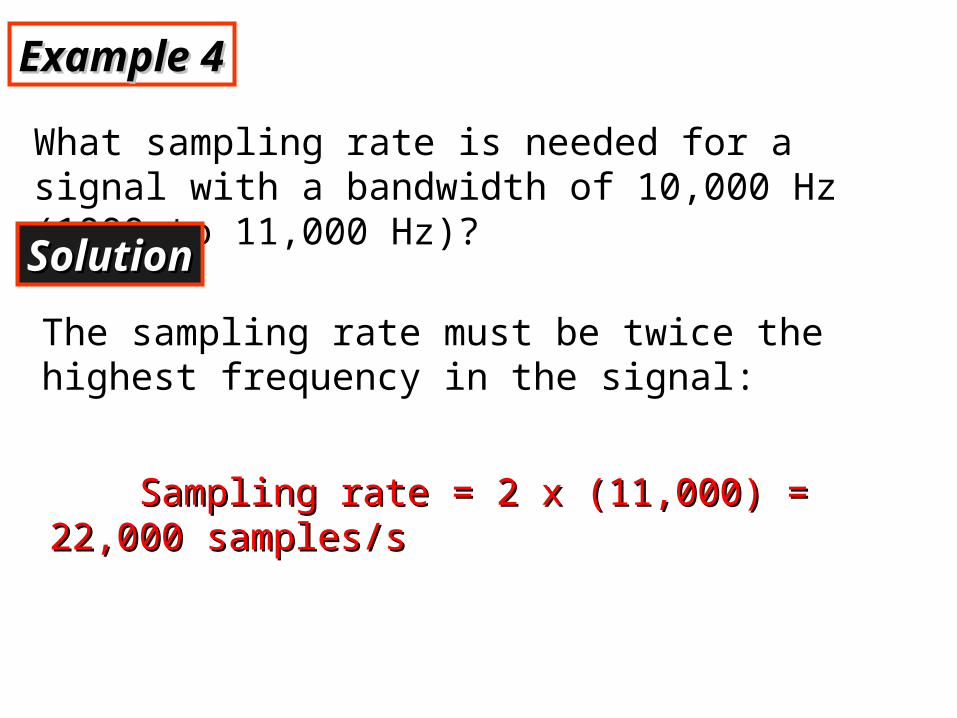
Example 4Example 4

What sampling rate is needed for a signal with a bandwidth of 10,000 Hz (1000 to 11,000 Hz)?

SolutionSolution

The sampling rate must be twice the highest frequency in the signal:

Sampling rate = 2 x (11,000) = 22,000 samples/sSampling rate = 2 x (11,000) = 22,000 samples/s

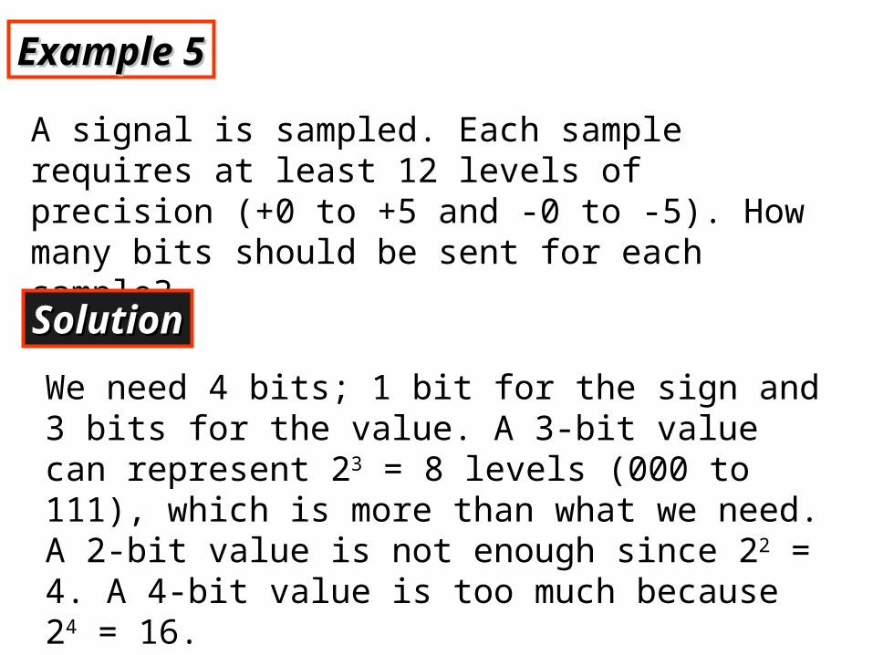
Example 5Example 5

A signal is sampled. Each sample requires at least 12 levels of precision (+0 to +5 and -0 to -5). How many bits should be sent for each sample?

SolutionSolution

We need 4 bits; 1 bit for the sign and 3 bits for the value. A 3-bit value can represent 23 = 8 levels (000 to 111), which is more than what we need. A 2-bit value is not enough since 22 = 4. A 4-bit value is too much because 24 = 16.

Example 6Example 6

We want to digitize the human voice. What is the bit rate, assuming 8 bits per sample?

SolutionSolution

The human voice normally contains frequencies from 0 to 4000 Hz. Sampling rate = 4000 x 2 = 8000 samples/sSampling rate = 4000 x 2 = 8000 samples/s

Bit rate = sampling rate x number of bits per sample Bit rate = sampling rate x number of bits per sample = 8000 x 8 = 64,000 bps = 64 Kbps= 8000 x 8 = 64,000 bps = 64 Kbps

4.4 Transmission Mode4.4 Transmission Mode

Parallel Transmission

Serial Transmission

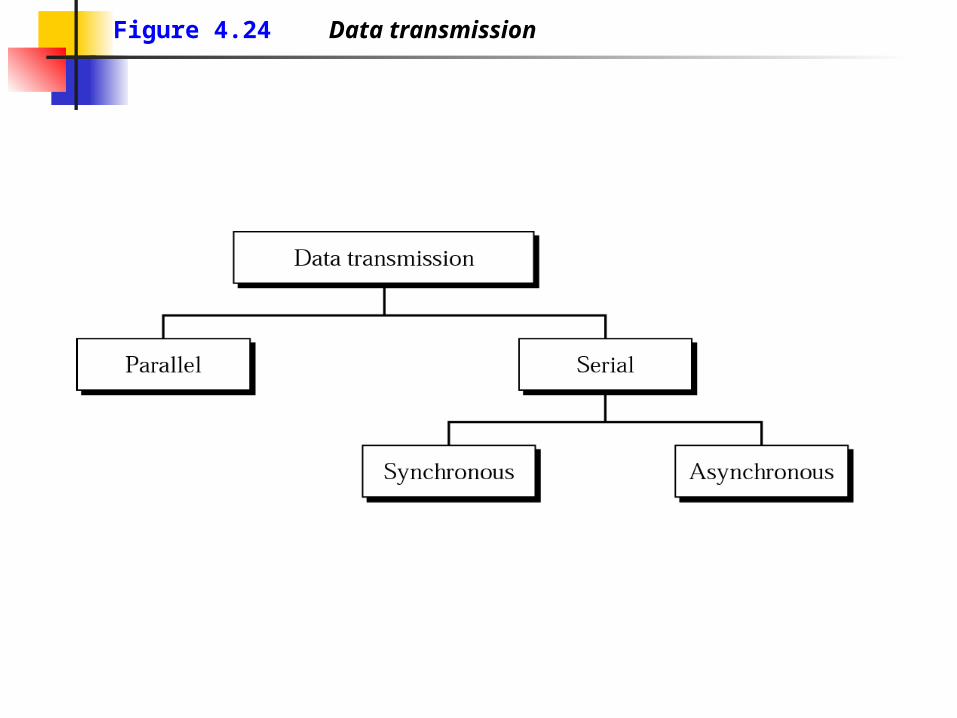
Figure 4.24 Data transmission

Figure 4.25 Parallel transmission

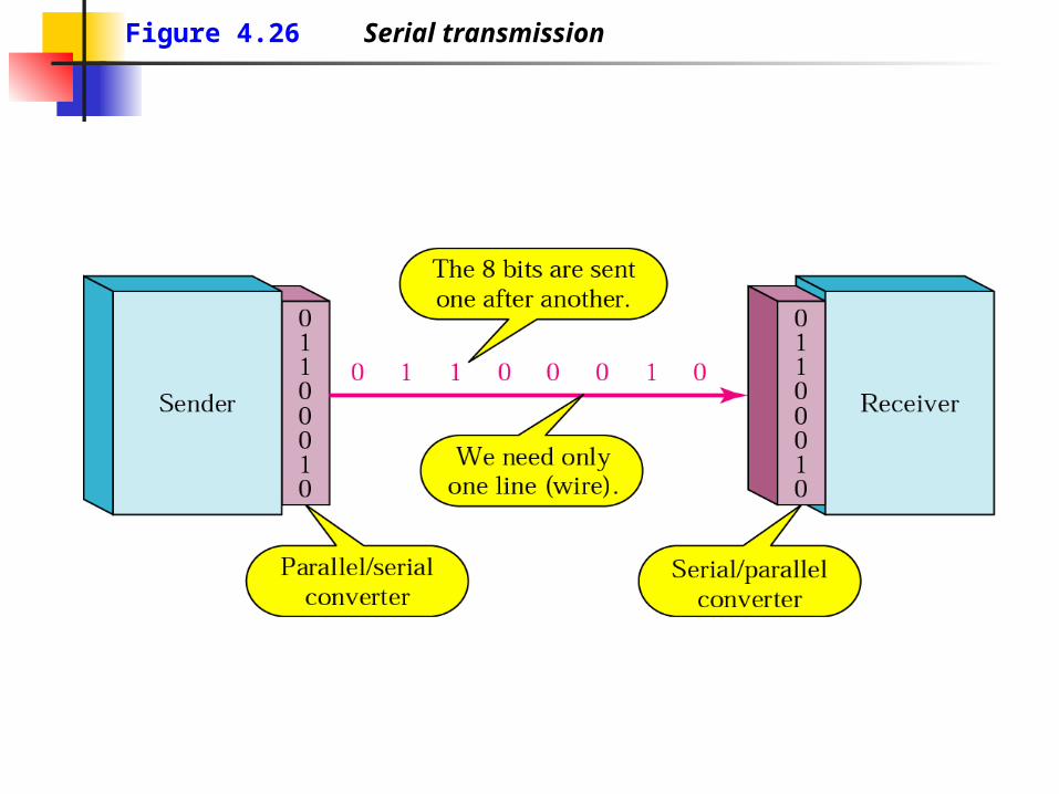
Figure 4.26 Serial transmission

In asynchronous transmission, we In asynchronous transmission, we send 1 start bit (0) at the beginning send 1 start bit (0) at the beginning

and 1 or more stop bits (1s) at the end and 1 or more stop bits (1s) at the end of each byte. There may be a gap of each byte. There may be a gap

between each byte.between each byte.

Note:Note:

Asynchronous here means Asynchronous here means “asynchronous at the byte level,” but “asynchronous at the byte level,” but the bits are still synchronized; their the bits are still synchronized; their

durations are the same.durations are the same.

Note:Note:

Figure 4.27 Asynchronous transmission

In synchronous transmission, In synchronous transmission, we send bits one after another without we send bits one after another without

start/stop bits or gaps. start/stop bits or gaps. It is the responsibility of the receiver to It is the responsibility of the receiver to

group the bits.group the bits.

Note:Note:

Figure 4.28 Synchronous transmission