Chapter 33 Electromagnetic waves Masatsugu Sei Suzuki Department of Physics, SUNY at Binghamton (Date: July 25, 2018) 1. Introduction In 1865, James Clerk Maxwell (1831 – 1879) provided a mathematical theory that showed a close relationship between all electric and magnetic phenomena. Maxwell’s equations also predicted the existence of electromagnetic waves that propagate through space. Einstein showed these equations are in agreement with the special theory of relativity. 0 E t B E 0 B 0 0 ( ) t E B J James Clerk Maxwell Born 13 June 1831 Edinburgh, Scotland, United Kingdom

Welcome message from author
This document is posted to help you gain knowledge. Please leave a comment to let me know what you think about it! Share it to your friends and learn new things together.
Transcript

Chapter 33
Electromagnetic waves
Masatsugu Sei Suzuki
Department of Physics, SUNY at Binghamton
(Date: July 25, 2018)
1. Introduction
In 1865, James Clerk Maxwell (1831 – 1879) provided a mathematical theory that
showed a close relationship between all electric and magnetic phenomena. Maxwell’s
equations also predicted the existence of electromagnetic waves that propagate through
space. Einstein showed these equations are in agreement with the special theory of
relativity.
0
E
t
B
E
0 B
0 0( )t
E
B J
James Clerk Maxwell
Born 13 June 1831
Edinburgh, Scotland, United Kingdom
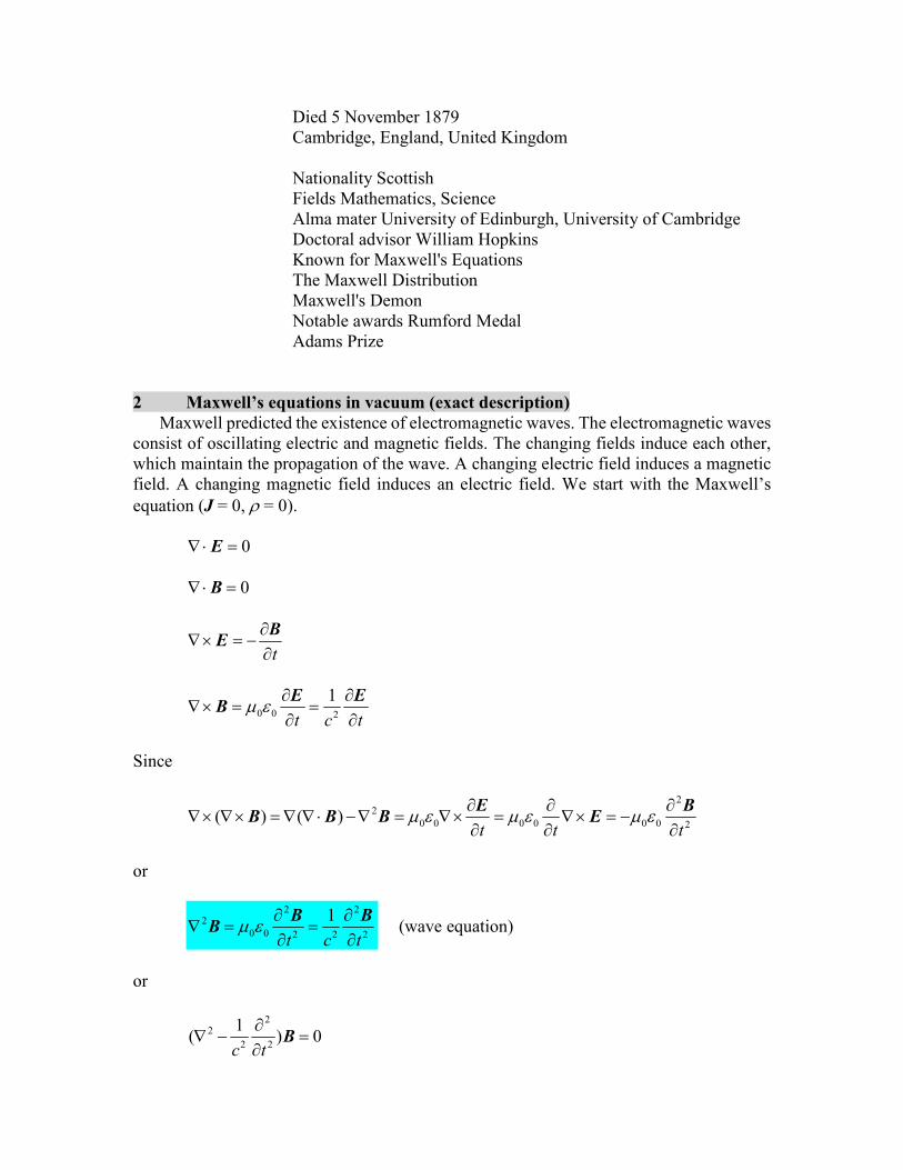
Died 5 November 1879
Cambridge, England, United Kingdom
Nationality Scottish
Fields Mathematics, Science
Alma mater University of Edinburgh, University of Cambridge
Doctoral advisor William Hopkins
Known for Maxwell's Equations
The Maxwell Distribution
Maxwell's Demon
Notable awards Rumford Medal
Adams Prize
2 Maxwell’s equations in vacuum (exact description)
Maxwell predicted the existence of electromagnetic waves. The electromagnetic waves
consist of oscillating electric and magnetic fields. The changing fields induce each other,
which maintain the propagation of the wave. A changing electric field induces a magnetic
field. A changing magnetic field induces an electric field. We start with the Maxwell’s
equation (J = 0, = 0).
0 E
0 B
t
B
E
0 0 2
1
t c t
E E
B
Since
2
2
0 0 0 0 0 0 2( ) ( )
t t t
E B
B B B E
or
2 2
2
0 0 2 2 2
1
t c t
B B
B (wave equation)
or
2
2
2 2
1( ) 0
c t
B

where c is the velocity of light,
00
1
c
Similarly,
2
2
0 0 2( ) ( ) ( )
t t
E E E B E
or
2 2
2
0 0 2 2 2
1
t c t
E E E (wave equation)
We consider the special case when E or B depends only on x. In this case the equation for
the field becomes
fx
cft 2
22
2
2
where f is understood any component of the vector E or B.
0))((
fx
ctx
ct
We introduce new variables
c
xt
c
xt
ttt
ccxxx
11
So that the equation for f becomes

02
f
The solution obviously has the form
)()( 21 fff
where f1 and f2 are arbitrary function.
or
)()( 21c
xtf
c
xtff
The function f1 represents a plane wave moving in the positive direction along the x axis.
The function f2 represents a plane wave moving in the negative direction along the x axis.
3. Plane-wave
3.1 Solutions for E and B
We are going to construct a rather simple electromagnetic field that will satisfy
Maxwell’s equation for empty space. We will assume that the vectors for the electric and
magnetic fields in an EM wave have a specific space-time behavior that is consistent with
Maxwell’s equations. The components of the electric and magnetic fields of plane
electromagnetic waves are perpendicular to each other and perpendicular to the direction
of propagation. This can be summarized by saying that electromagnetic waves are
transverse waves.
Suppose that E and B are described by a plane waves
0 cos( )t E E k r
0 cos( )t B B k r
where k is the wave number and is the angular frequency. The direction of k is the same
as that of the propagation of the wave.
(i) Step-1
From the wave equation
2
2
2 2
1
c t
E E
we have

22
0 02c
k E E
The angular frequency satisfies the dispersion relation given by
fc
ck
22
where
cf
k
f
2
2
(ii) Step-2
From
0 E , and 0 B
we have
0 0 k E , and 0 0 k B
The wave vector k is perpendicular to E and B.
(iii) Step-3
From
t
B
E
0 0( ) k E B
0 0( ) ck k E B
or
0 0ˆ( ) c k E B
or

0 0
1 ˆ( )c
B k E
Note that
00 cBE
Fig. A linearly polarized, sinusoidally varying plane wave propagating
in the positive x direction. The figure represents a snapshot at a
particular time. This figure is made by using the ParametricPlot3D
of the Mathematica.
((Conclusion))
The solutions of Maxwell’s equation are wave-like, with both E and B satisfying a
wave equation. Electromagnetic waves travel at the speed of light. This comes from the
solution of Maxwell’s equations. Waves in which the electric and magnetic fields are
restricted to being parallel to a pair of perpendicular axes are said to be linearly polarized
transverse waves. The direction of the wave’s polarization coincides with that of the
electric field.
3.2 Energy density and Poynting vector in electromagnetic wave (exact
description)
Electromagnetic waves carry energy. As they propagate through space, they can
transfer that energy to objects in their path. The rate of flow of energy in an electromagnetic
(EM) wave is described by a vector called the Poynting vector.
The energy density u is given by
2 2
0
0
1 1( )
2u
E B
The Poynting vector S is given by

0
1( )
S E B
(a) The time-averaged energy density <u>
First we calculate the time average of 2E
2 2 2
0 cos ( )t E E k r
The time average of 2E
2 2 2 2
0
0 0
2
0
0
2
0
1 1cos ( )
1[1 cos(2 2 )]
2
1
2
T T
rms
T
E dt E t dtT T
E t dtT
E
E k r
k r
The root-mean square value of the electric field is given by
max02
1
2
1EEErms
where E0 = Emax, 2
T , and 0
1cos(2 2 ) 0
T
t dtT
k r
Similarly, we have
2 2 2
0
0
1 1
2
T
rmsB dt BT
B ,
The root-mean square value of the magnetic field is
max02
1
2
1BBBrms
where B0 = Bmax,
ckB
E
B
E
rms
rms
max
max
Then the time-average of the energy density is given by

)1
(4
1)
1(
2
1 2
0
0
2
00
2
0
2
0 BEBEu rmsrms
Here we note
2
02
2
0
1E
cB
Then we have
2
0
2
00
2
02
0
2
002
1)
1(
4
1rmsEEE
cEu
(b) The time-averaged Poynting vector <S>
Next we calculate the Poynting vector S
2
0 0
0 0
1 1( ) ( ) cos ( )t
S E B E B k r
The time-averaged Poynting vector <S> is obtained as
0 0
0
1( )
2 S E B

Noting that
2
0 0 0 0 0
1 1ˆ ˆ( ) Ec c
E B E k E k
we have
2
0
0
1 1ˆ2
Ec
S k
or
2 200 02
0
1 1ˆ ˆ ˆ2 2
c E c E c uc
S k k k
where k̂ is the unit vector of the wave vector k, ˆk
k
k , and
ucS
(c) The intensity I (= <S>)
Here we define the intensity I of the light. The intensity I is the energy flux (energy per
unit area per unit time);
I = <S>.
We now consider the photon flows (photon is the quantization of light with the velocity c)
flows. During the time t , the total energy passing through the area A is
utcAuVU
where the volume V is tAc and the energy density is u . From the definition of <S>, the
total energy passing through the area A during the time t, is given by
StAU
area 1
photons
ℏ
ct

Then we have
StAutcAU ,
leading to
2
0
2
max
0
2
0
0
2
00
1
2
1
2
1
2
1rmsE
cE
cE
cEcucS
tA
UI
where the unit of the intensity I is J/m2 s = W/s.
((Note))
Poynting, John Henry (1852-1914)
English physicist, mathematician, and inventor. He devised an equation by which the
rate of flow of electromagnetic energy (now called the Poynting vector) can be determined.
In 1891 he made an accurate measurement of Isaac Newton's gravitational constant.
Poynting was born near Manchester and studied there at Owens College, and at Cambridge.
From 1880 he was professor of physics at Mason College, Birmingham (which became
Birmingham University in 1900). In On the Transfer of Energy in the Electromagnetic
Field 1884, Poynting published the equation by which the magnitude and direction of the
flow of electromagnetic energy can be determined. This equation is usually expressed as S
= (1/0)ExB where S is the Poynting vector, is the permeability of the medium, E is the
electric field strength, B is the magnetic field strength, and is the angle between the vectors
representing the electric and magnetic fields. In 1903, he suggested the existence of an
effect of the Sun's radiation that causes small particles orbiting the Sun to gradually
approach it and eventually plunge in. This idea was later developed by US physicist
Howard Percy Robertson (1903-1961) and is now known as the Poynting-Robertson effect.
Poynting also devised a method for measuring the radiation pressure from a body; his
method can be used to determine the absolute temperature of celestial objects. Poynting's
other work included a statistical analysis of changes in commodity prices on the stock
exchange 1884.
4. Physical meaning of Maxwell’s equation
(a)
t
B
E , or Bdt
E s�

Fig. A time-varying B-field. Surrounding each point where the magnetic flux B is
changing the E-field forms closed loops.
(b)
tc
E
B2
1, or
2
1Ed
c t
B s�

Fig. A time-varying E-field. Surrounding each point where E is changing the B-field
forms closed loops.
A time-varying E-field generates a B-field which is everywhere perpendicular to the
direction in which E-field changes. In the same way, a time-varying B-field generates an
E-field which is everywhere perpendicular to the direction in which B-field changes. One
can anticipate the general transverse nature of the E- and B-fields in an electromagnetic
disturbance.

7. Energy conservation: Poynting theorem
We consider a general case where J and are not zero. The system consists of charged
particles and the fields E and B.
Fig. Combined system (particle and fields) inside volume V.

The work energy theorem:
K W t F r F v
where K is the kinetic energy and F is the Lorentz force and is given by
[ ( )]V V F f E v B
where f is the force density,
[ ( )] f E v B .
Then we have
[ ( )] ( ) ( )W V t V t V t E v B v E v E J
or
1 W
V t
E J
where
J v
More generally
dWd
dt E J
((Poynting theorem))
The work done on the changes by the electromagnetic force is equal to the decrease in
energy stored in the field, less the energy that flows out through the surface.
( )dW d d
d ud d ud ddt dt dt
E J S S a
0d
ud d ddt
S a E J (Energy conservation)
The first term: the rate of change of the total energy of the electromagnetic field in
volume V.
The second term the rate at which the electromagnetic field energy flows out through
surface.

The third term the rate at which the field is doing work on the charges.
The above equation can be rewritten as
0u
d d dt
S E J
or
0u
t
S E J
using the Gauss’ law.
8. Example of the Poynting theorem
8.1 Energy flow in conduction
Here we show that the energy that ends up as joule heating is carried by the
electromagnetic field outside the wire.
For simplicity we consider a DC current I flowing along a long straight wire of radius a
and length L. The electric field E is given by
0 ˆV
zL
E
Then we have
2002
V
V IdV a L V I
L a
E J
The magnetic field on the surface of the wire is

0 ˆ2
I
a
B .
The Poyinting vector is
0 0 0
0 0
1 1ˆ ˆˆ( )
2 2
V I V Iz r
L a aL
S E B
The rate of transport energy through the lateral surface is
0 00
ˆ 22 2
V I V Id r d aL IV
aL aL
S a a� �
Then we have
0V
dV d E J S a�
Note that E and B are independent of t. It means that the energy density u is independent
of t,
0dt
u
Hence the Poyting’s theorem is satisfied. The electromagnetic energy flow into the wire
from its sides is converted into kinetic (heat) energy within the wire.
8.2 Energy flow in capacitance
We consider the second case where E and B are dependent on time.
( )dW d d
d ud d ud ddt dt dt
E J S S a

There is a displacement current in the space between two plates.
0 0t
E
B
2
0 0( ) 2dE
d d B s sdt
B a B l� �
dt
dEss
dt
dE
sB
22
1 002
00
The Poynting vector S on the cylinder surface is
0 00
0 0
1
2 2z s
dE a dEE a E
dt dt
E B
S e e e
The total amount of flow through the whole surface between the edges of the plate.
2 2
0 0
12 (2 ) ( )
2 2
a dE dd ahS ah E a h E
dt dt S a

Since the current i is related to the charge Q by
dt
dQi
we have
2
0 0
z z
Q
a
E e e .
The potential difference between two plates is
C
Q
a
QhEhV
0
2,
where the capacitance C is given by
Ch
a0
2.
The energy density u is
2 2
0
0
1 1( )
2u
E B
The total energy U is
])4
(2
1
2
1[2)2(
2
3
2
0
2
0
0
2
0
0
dt
dEsEsdshdssuhudU
a
or
])44
(2
1
2
1
2[2
242
0
2
0
0
2
0
2
dt
dEaE
ahU
or
]8
1[
2
2
22
00
2
0
2
dt
dEaE
haU
2
22
00
4
0
2
8 dt
Ed
dt
dEha
dt
dEEha
t
U

Energy conservation (Poynting theorem)
dW dd U d
dt dt E J S a
The right-hand side of this equation is defined by K1. K1 is evaluated as follows.
4 2
2 2 2 2 2
1 0 0 0 02
1 1[ ( ) ] ( )
2 8 2
d d a h dE d E dK U d a h E a h E
dt dt dt dt dt
S a
or
2
22
00
4
18 dt
Ed
dt
dEhaK
Since
0
2a
QE
we have
0
2
0
2
1
a
I
dt
dQ
adt
dE
dt
dI
adt
Ed
0
22
2 1
.
Then dt
dWcan be rewritten as
dt
dII
h
dt
Ed
dt
dEhaK
dt
dW02
22
00
4
188
When )cos(0 tII ,
)2sin(16
2
00 tI
h
dt
dW
The time-averaged of dW/dt is

0dt
dW
over a period T.
9. Summary From Lecture Notes from Walter Lewin 8.02 Electricity and
Magnetism
2
0
1
2Eu E (J/m3)
2
0
2
0
1
2
1
2
B
E
u B
E
c
u
(J/m3)
where E cB , 0 0
1c
The total energy density is
2
0 0u E cEB .
The energy passing through unit area (1 m2) per second is
2 2
0
0 0
1 1cu c EB EB E
c
(J/m2 s)
The time average:
2 2
0 0 0
0 0 0
1 1 1
2 2rmsc u E B E E
c c
The Poynting vector:
0
1
S E B (W/m2)
where W=J/s. The time average is

2 2
0 0 0
0 0 0
1 1 1
2 2rmsS E B E E
c c
or
S c u
where 0
1
2rmsE E
((Example))
(a) E0 = 100 V/m
2
0
0
113.2721
2S E
c W/m2
(b) E0 = 1000 V/m
2
0
0
11327.21
2S E
c W/m2
(c) Solar constant
21361.17
4 u
SA
L
� W/m2 (Solar constant)
where
111.4959787 10uA m, (distance between the sun and the earth)
L☉ = 3.828 x 1026 W (Solar luminosity)
Note that
0 02 1012.71E c S V/m
Poynting vector
S c u
where p is the momentum of photon and momP is the momentum of the system

cp , (energy dispersion of photon)
The total energy is given by
( )( ) momU u A c t cP
Thus we get the relation between the radiation pressure and
momrad
cPS c u cP
A t
or
rad
SP
c
In general
rad
SP
c
where = 1 for full absorption, 0 for the transparency, and 2 for the reflection (metal).
Radiation pressure is the pressure exerted upon any surface due to the exchange of
momentum between the object and the electromagnetic field. This includes the momentum
of light or electromagnetic radiation of any wavelength which is absorbed, reflected, or
otherwise emitted (e.g. black body radiation) by matter on any scale (from macroscopic
objects to dust particles to gas molecules).
10. Derivation of the relation 0 0 0 0B cE
A part of this topics was discussed in the lecture of Prof. Walter Lewin (MIT 8.02
Electricity and Magnetism 2004).
(a) Method-I (from the Ampere-Maxwell law)
radP

0 0 0 0( ) d d dt t
E
B a B l E a� � �
d EE a�
/4
0
0
cos( )ldzE kz t
E
/4
0
0
/4
0
0
/4
0
0
cos( )
( 1)( ) sin( )
sin( )
ldzE kz tt t
ldzE kz t
lE dz kz t
E

/4
/400 0 0 0
0
| sin( ) [ cos( )] |t
ElE dz kz l kz lcE
t k
E
Ampere’s law:
0 0 0 0B l lcE
leading to
0 0 0 0 0
1B cE E
c
(b) Method II (from the Faraday’s law)
________________________________________________________________________
______

( ) Bd d dt t
E a E l B a� � �
d B B a�
/4
0
0
cos( )ldzB kz t
B
/4
0
0
/4
0
0
/4
0
0
cos( )
( 1)( ) sin( )
sin( )
ldzB kz tt t
ldzB kz t
lB dz kz t
B
/4
/400 0 0 0
0
| sin( ) [ cos( )] |t
BlB dz kz l kz lcB
t k
B
Faraday’s law:
0 0E l lcB , or 0 0E cB
leading to
0 0 0 0 0
1B cE E
c
11. Momentum conservation
We start with the expression of the pointing vector,
0 0
1 1( ) ( )
t t t t
ES E B B E B
Here we only use the Maxwell’s equation.
0
0 0
1( )
t
t
BE
EB J

Then we have
0 0
0 0
1( ) ( )
t t t
ES B E B B J B E E
leading to the momentum conservation,
0 0 Tt
S f�
(momentum conservation)
or
2
1T
c t
S f
�
where Tij is called the Maxwell stress tensor,
2 2
0 0
0 0
1 1 1( )2 2
ij ij i j i jT E E B B
E B
2 2
0 0
, , ,0 0
,
1 1 1( ) ( ) ( )2 2
j ji ii ij j i i j i i
i j i j i jj j j j j
ji i
i j j
E BE BT E E B B
x x x x x
Tx
e E B e e
e
�
12. Momentum of the field, momentum density
12.1 Definition
The pointing vector S gives not only the energy flow but, if it is divided by c2, also the
momentum density.
For particles, we have
mech t V t P F f
( mechP : the total momentum of all the particles in a volume V)
or
1 mech
V t
P
f E J B
or
mecdd
dt
Pf (in general)

Here we define the momentum of the field (per unit volume), the momentum density as
0 0 2
1
c G S S (momentum density)
em d P G
where emP is the total electromagnetic momentum stored in the electromagnetic field.
We now consider the physical meaning.
0 0 Tt
S f�
(momentum conservation)
or
( ) ( )d T d T dt
G f a
� �
or
( )em mech T dt
P P a�
where
mech dt
Pf F
ememd
t t
P
G F
The impulse Iem is defined by
em em emt I F P
((Note)) Definition of mass density
2200
1
c
ucS
cSG
The mass density is defined as

2c
u , or 2cu
which is the main result of relativistic theory (Einstein).
12.2 Correspondence
The following table shows the correspondence between the particles and fields.
Particles E-B fields
2
1
cG S (momentum ensity)
Pmech em d P G (momentum)
f 2
1
t c t
G S
(force density)
mechmech
dd
dt
PF f em
em
dd
t dt
PF G (force)
mech mech mech t I P F em em em t I P F (impulse)
13. Radiation pressure
Radiation pressure is the pressure exerted upon any surface exposed to electromagnetic
radiation. For example, the radiation of the Sun at the Earth has an energy flux density of
1370 W/m2, so the radiation pressure is 4.6 µPa (absorbed).
Here we consider the two cases: the absorption and reflection of light waves at a surface
of the object.

(1) Total absorption
The momentum Pem is delivered to the object. I is the impulse.
emem
em em em
t
t
PF
I F P P
where
2em Ac t Ac tc
S
P G
where A is the area.
((Note)) G[(J s/m)/ m3], A[m2], tGAc [(J s/m)/ m3][m2][m/s][s]=[J.s/m]
Then we have the impulse and the force given by
2
0
em em
emem
P Ac tc
P IA A
t c c
SI
SF
since 0I c u S (the intensity) and I0 is the intensity of the light wave.
The radiation pressure is given by
c
I
A
Fem 0
(2) Total reflection
area 1
photons
ℏ
ct

2
0
2 2
22 2
em em
em
t Ac tc
IA u A A
c c
SI F P P
SF
since 0I c u S (the intensity)
The radiation pressure is
c
I
A
Fem 02
((Radiation pressure on the tails of comets))
The minute pressure exerted on a surface at right-angles to the direction of travel of the
incident electromagnetic radiation. Its existence was first predicted by James Maxwell in
1899 and demonstrated experimentally by Peter Lebedev. In quantum mechanics, radiation
pressure can be interpreted as the transfer of momentum from photons as they strike a
surface. Radiation pressure on dust grains in space can dominate over gravity and explains
why the tail of a comet always points away from the Sun.

(3) Partial reflection and absorption
Problem 33-23; partial absorption and partial reflection
Prove, for a plane electromagnetic wave that is normally incident on a flat surface, that
the radiation pressure on the surface is equal to the energy density in the incident beam.
(This relation between pressure and energy density holds no matter what fraction of the
incident energy is reflected.
Let f be the fraction of the incident beam intensity that is reflected. The fraction
absorbed is 1 – f. The reflected portion exerts a radiation pressure of
c
fIpr
02
and the absorbed portion exerts a radiation pressure of
c
Ifpa
0)1(
where I0 is the incident intensity. The factor 2 enters the first expression because the
momentum of the reflected portion is reversed. The total radiation pressure is the sum of
the two contributions:
c
If
c
IffIppp artotal
000 )1()1(2
To relate the intensity and energy density, we consider a tube with length ℓ and cross-
sectional area A, lying with its axis along the propagation direction of an electromagnetic
wave. The electromagnetic energy inside is U uA ℓ, where u is the energy density. All
this energy passes through the end in time t c ℓ / , so the intensity is
cuAl
Alcu
At
UI
Thus u = I/c. The intensity and energy density are positive, regardless of the propagation
direction. For the partially reflected and partially absorbed wave, the intensity just outside
the surface is
000 )1( IffIII
where the first term is associated with the incident beam and the second is associated with
the reflected beam. Consequently, the energy density is

c
If
c
Iu 0)1(
the same as radiation pressure.
14. Electromagnetic waves
Table shows the frequency and wavelength of the light ranging from the gamma ray to
the AM wave.

15. Polarization
The electric and magnetic vectors associated with an electromagnetic wave are
perpendicular to each other and to the direction of wave propagation. Polarization is a
property that specifies the directions of the electric and magnetic fields associated with an
EM wave. The direction of polarization is defined to be the direction in which the electric
field is vibrating.

The plane containing the E-vector is called the plane of oscillation of the wave. Hence the
wave is said to be plane polarized in the y direction. We can represent the wave’s
polarization by showing the direction of electric field oscillations in a head-on view of the
plane of oscillation.
16 Unpolarized light
All directions of vibration from a wave source are possible. The resultant EM wave is
a superposition of waves vibrating in many different directions. This is an unpolarized
wave. The arrows show a few possible directions of the waves in the beam. The
representing unpolarized light is the superposition of two polarized waves (Ex and Ey)
whose planes of oscillation are perpendicular to each other.

17. Intensity of transmitted polarized light
(1) Malus’ law
An electric field component parallel to the polarization direction is passed (transmitted)
by a polarizing sheet. A component perpendicular to it is absorbed.

The electric field along the direction of the polarizing sheet is given by
cosEEy
Then the intensity I of the polarized light with the polarization vector parallel to the y axis
is given by
2
0 cosII (Malus’ law)
where
2
0
0
2
cosIc
ESI rms
avg
((Note)) Etienne Louis Malus (1775 – 1812).
(2) One-half rule for unpolarized light
When the light reaching a polarization sheet is unpolarized, we get a polarized light
with the intensity
2
0II (one-half rule)
since
2)]2cos(1[
2
1
2cos
2
1 02
0
02
0
2
0
Id
IdII

((Example)) Problem 33-74
In Fig., unpolarized light with an intensity I0 (25 W/m2) is sent into a system of four
polarising sheet with polarizing directions at angles 1 = 40°, 2 = 20°, 3 = 20°, and 4 =
30°. What is the intensity of the light emerges from the system?
((Solution))
1 = 40°
2 = 20°
3 = 20°

4 = 30°
I0 = 25 W/m2
The intensity is given by
2
222
43
2
32
2
21
20
43
2
32
2
21
20
/504.0
)50(sin)40(cos)20(sin2
25
)(sin)(cos)(sin2
)90(cos)180(cos)90(cos2
mW
I
II
18. Index of refraction
The velocity of the light in the material with and
n
cv
1
Here n is the index of refraction;
00
n
For most materials, 0
19. Reflection and transmission

((First law))
The incident, reflected, and transmitted wave vectors form a plane (plane of incidence),
which also includes the normal to the surface.
((Second law))
Ri
((Third law))
1
2
sin
sin
n
n
T
i
(Snell’s law)
Willebrod Snell (1591 – 1626)
20. Dispersion
For a given material, the index of refraction varies with the wavelength of the light
passing through the material. This dependence of n on is called dispersion. Snell’s Law
indicates light of different wavelengths is bent at different angles when incident on a
refracting material
21. Prism

The ray emerges refracted from its original direction of travel by an angle , called the
angle of deviation. depends on the apex angle of the prism and the index of refraction
n of the material. Since all the colors have different angles of deviation, white light will
spread out into a spectrum.
(a) Violet deviates the most.
(b) Red deviates the least.
(c) The remaining colors are in between.
AB and AD are the surface of the prism. is the vertex angle of the prism and is the
deviation angle. From the geometrical consideration, the points A, B, C, and D are on the
same circle. Then we have the following relations,
21
2211
21
)()(
ii
titi
tt
.
Snell's law:
11 sinsin ti n , 22 sinsin ti n
where n is the index of refraction of the prism.
((Angle of minimum deviation))
Here we discuss the angle as a function of the incident angle i1. From the Snell’s
law,

)sincoscos(sin)sin(sinsin 11122 tttti nnn .
We note that
n
n
it
itt
11
1
2
21
2
1
sinsin
sin1
1sin1cos
.
Then we get
11
22
11
2
22
sincossinsin
sincossin
11sinsin
ii
iii
n
nn
nn
.
The angle of deviation is obtained as
)sincossinarcsin(sin 11
22
1 iii n .
Here we assume that = 60º. We make a plot of the angle as a function of i1, where the
index of refraction n is changed as a parameter. It is found from the figure that takes
minimum at a characteristic angle (the angle of minimum deviation),
)]2
sin(arcsin[1
ni .
Fig. Deviation vs incident angle, where n is changed as a parameter.
What is the condition for the angle of minimum deviation? The condition is derived as

21
21
tt
ii
(symmetric configuration)
In other words, the ray BD should be parallel to the base of the prism (the isosceles triangle
with the apex angle ) in the case of the angle of minimum deviation.
((Proof))
The angle has a minimum at the angle of minimum deviation,
01
id
d
,
or
12 ii dd , (1)
From 21 tt , we have
21 tt dd . (2)
From the Snell's law,
2222
1111
coscos
coscos
ttii
ttii
dnd
dnd
. (3)
From Eqs.(1), (2), and (3), we have
2
22
1
22
2
2
1
2
2
2
2
1
2
2
2
1
2
1
sin
sin
sin1
sin1
sin1
1
sin1
1
cos
cos
cos
cos
i
i
i
i
i
i
t
t
i
i
n
n
n
n
,
which leads to the condition given by
221
21
tt
ii
.

Using this condition, the incident angle can be calculated as
)]2
sin(arcsin[1
ni .
When = 60º, we have
59.481i for n = 1.50
13.531i for n = 1.60
21.581i for n = 1.70
((Example)) Problem 33-55
Index of refraction n, the angle of minimum deviation
In Fig., a ray is incident on one surface of a triangular glass prism in air. The angle of
incidence is chosen so that the emerging ray also makes the same angle with the normal
to the other face. Show that the index of refraction n of the glass prism is given by
2sin
2sin
n
where is the vertex angle of the prism and is the deviation angle, the total angle through
which the beam is turned in passing through the prism. (Under these conditions, the
deviation angle has the smallest possible value, which is called the angle of minimum
deviation).

((Solution))
From the symmetry, the points A, B, C and D are on the same circle. The line CD is
the diameter of the circle. Note that an angle inscribed in a semicircle is a right angle.
Snell’s law:
1sinsin n
We also have the relations
)(2 1
and
12
which leads to the expression given by
2
Then the index of refraction n is derived as
2sin
2sin
n
22. Brewster’s angle: Polarization without polarizer
Figure shows a ray of unpolarized light incident on a glass surface. Let us resolve the
electric field vectors of the light into two components. The perpendicular components are
perpendicular to the plane of incidence and thus also to the page in Fig.; these components
are represented with dots (as if we see the tips of the vectors). The parallel components are
parallel to the plane of incidence and the page; they are represented with double-headed
arrows. Because the light is unpolarized, these two components are of equal magnitude.
A ray of unpolarized light in air is incident on a glass surface at the Brewster angle θB.
The electric fields along that ray have been resolved into components perpendicular to the
page (the plane of incidence, reflection, and refraction) and components parallel to the page.
The reflected light consists only of components perpendicular to the page and is thus
polarized in that direction.
The refracted light consists of the original components parallel to the page and weaker
components perpendicular to the page; this light is partially polarized

Scottish physicist, Sir David Brewster (1781-1868)
(A) Reflection and transmission for the polarization vector in the plane of
incidence (application of the Fresnel’s equations)
The polarization of the incident wave is parallel to the plane of incidence. The reflected
and transmitted waves are also polarized in this plane.
Then we have two independent equations. Here we define
22
11
cos
cos
v
v
I
T

Reflection coefficient
2
//
I
R
I
IR
Transmission coefficient
2
2
//)(
42
I
T
I
IT
where // means that the polarization vector is in the plane of incidence.
(B) Reflection and transmission for the polarization vector perpendicular to the
plane of incidence (application of the Fresnel’s equations)
Reflection coefficient
2
1
1
I
R
I
IR
Transmission coefficient
2)1(
4
I
T
I
IT
where means that the polarization vector perpendicular to the plane of incidence.

We now consider the case when 21
T
I
I
T
n
n
v
v
v
v
sin
sin
cos
cos
1
2
2
1
22
11
Then we have
////
22
//
1
)2sin()2sin(
)2sin()2sin(
RT
RIT
IT
RT
RIT
IT
1
)(sin
)(sin
1
12
22
Note that 0// R for )2sin()2sin( IT . This means that
IT 22 or IT 22
or
2
IT (Brewster angle).
Using the Snell’s law, we have

III nnn
cos)2
sin(sin 221
then we have a Brewster’s angle (I), which is defined by
1
2tann
nI
R// (red), T//(orange), R (yellow), T(green)
R+T =1
((Experiment)) Brewster angle
You need only a polarizer for this experiment. Suppose that sun light enters from
outside through a window and is reflected on the floor of your class room. When you look
at the reflected light using the polarizer and slowly rotates the polarizer in one direction,
you may easily find that the unpolarized light is polarized at some angle (that is a Brewster
angle).
((Feynman)) From “Surely you are joking, Mr Feynman”
Surely you are joking Mr. Feynman
Brewster angle for the polarization of light
In regard to education in Brazil, I had a very interesting experience. I was teaching a
group of students who would ultimately become teachers, since at that time there were
not many opportunities in Brazil for a highly trained person in science. These students
had already had many courses, and this was to be their most advanced course in
electricity and magnetism - Maxwell's equations, and so on.
The university was located in various office buildings throughout the city, and the
course I taught met in a building which overlooked the bay. I discovered a very strange
phenomenon: I could ask a question, which the students would answer immediately. But
the next time I would ask the question - the same subject, and the same question, as far as
I could tell - they couldn't answer it at all!
20 40 60 80
0.2
0.4
0.6
0.8
1

For instance, one time I was talking about polarized light, and I gave them all some
strips of polaroid. Polaroid passes only light whose electric vector is in a certain direction,
so I explained how you could tell which way the light is polarized from whether the
polaroid is dark or light. We first took two strips of polaroid and rotated them until they let
the most light through. From doing that we could tell that the two strips were now admitting
light polarized in the same direction - what passed through one piece of polaroid could also
pass through the other. But then I asked them how one could tell the absolute direction of
polarization, for a single piece of polaroid. They hadn't any idea. I knew this took a certain
amount of ingenuity, so I gave them a hint: "Look at the light reflected from the bay
outside." Nobody said anything. Then I said, "Have you ever heard of Brewster's Angle?".
"Yes, sir! Brewster's Angle is the angle at which light reflected from a medium with an
index of refraction is completely polarized." "And which way is the light polarized when
it's reflected?" "The light is polarized perpendicular to the plane of reflection, sir." Even
now, I have to think about it; they knew it cold! They even knew the tangent of the angle
equals the index! I said, "Well?" Still nothing. They had just told me that light reflected
from a medium with an index, such as the bay outside, was polarized; they had even told
me which way it was polarized. I said, "Look at the bay outside, through the polaroid. Now
turn the polaroid." "Ooh, it's polarized!" they said.
After a lot of investigation, I finally figured out that the students had memorized
everything, but they didn't know what anything meant. When they heard "light that is
reflected from a medium with an index," they didn't know that it meant a material such as
water. They didn't know that the "direction of the light" is the direction in which you see
something when you're looking at it, and so on. Everything was entirely memorized, yet
nothing had been translated into meaningful words. So if I asked, "What is Brewster's
Angle?" I'm going into the computer with the right keywords. But if I say, "Look at the
water," nothing happens they don't have anything under "Look at the water"!
23. Total internal reflection
A phenomenon called total internal reflection can occur when light is directed from a
medium having a given index of refraction toward one having a lower index of refraction

Fig. The total internal reflection of light from a point S, occurs for all angles of incidence
greater than c. In this case c = arcsin(1/n) = 41.8° for n = 1.50. At c, the refracted
ray points along the air-glass interface.
Possible directions of the beam are indicated by rays numbered 1 through 5. The refracted
rays are bent away from the normal since n1 > n2.
Critical angle, c

There is a particular angle of incidence that will result in an angle of refraction of 90°.
This angle of incidence is called the critical angle, c.
1
2sinn
nc
24. Birefringence
We observe a birefringence in calcite.

25. Typical problems
Formula
0
2
0
2
22 mm cB
c
EI
c = 2.99792458 x 10⁸ m/s
0 = 12.566370614 x 10⁻⁷ (H/m)
0 = 8.854187817 x 10⁻¹² (F/m)
Em = c Bm

mrms
mrms
BB
EE
2
1
2
1
ckB
E
B
E
rms
rms
max
max
cIu / energy density
Pr = I/c radiation pressure for the total absorption
Pr = 2I/c radiation pressure for the totale reflection
25.1 Problem 33-15
Sunlight just outside Earth’s atmosphere has an intensity of 1.40 kW/m2. Calculate (a)
Em and (b) Bm for sunlight there, assuming it to be a plane wave.
((Solution))
I = 1.40 kW/m2
c
EI m
0
2
2
or
cIEm 02 1.03 x 10³ V/m
c
EB m
m = 3.43 x 10⁻⁶ T
25.2 Problem 33-31(Sp-33) radiation pressure
As a comet swings around the Sun, ice on the comet’s surface vaporized, releasing
trapped dust particles and ions. The ions, because they are electrically charged, are forced
by the electrically charged solar wind into a straight ion tail that points radially away from
the Sun (Fig). The (electrically neutral) dust particles are pushed radially outward from the
Sun by the radiation force on them from sunlight. Assume that the dust particles are
spherical, have density 3.5 x 10³ kg/m3, and are totally absorbing. (a) What radius must a
particle have in order to follow a straight path, like path 2 in the figure? (b) If its radius is
larger, does its path curve away from the Sun (like path 1) or toward the Sun (like path 3)?
((Solution))

dust particle
spherical
= 3.5 x 10³ kg/m3
Totally absorbing
(a)
The radiation pressure:
c
IPem
where
24 r
PI
Then the force due to the radiation pressure,
2
2
2
22
44)(
1)(
cr
PR
r
PR
cR
c
IAPF emem
The central force due to the gravitation,
)3
4( 3
22
R
r
GM
r
GmMF sunsun
g

From the condition that Fg = Fem
mGMc
PRR
Rr
GM
cr
PR
sun
c
sun
7
3
22
2
107.116
3
3
4
4
(path-2)
(b)
)3
4(
4
3
2
2
2
Rr
GMF
cr
PRF
sung
em
For R>Rc, Fg>Fem. (path-3)
For R<Rc, Fg<Fem. (path-1)
25.3 Problem 33-75 Snell’s law
(a) Prove that a ray of light incident on the surface of a sheet of plate glass of thickness
t emerges from the opposite face parallel to its initial direction but displaced sideway, as
in Fig. (b) Show that, for small angles of incidence , this displacement is given by
)1
(n
ntx
,
where n is the index of refraction of the glass and q is measured in radians.

((Solution))
Snell’s law
1
1sinsin
n
n
From the geometry,
)1
1(
)(
tan)tan(
1
1
nt
t
ttx
25.4 Problem 33-89 Plane wave
The magnetic component of a polarized wave of light is
])1057.1sin[()100.4( 176 tymTBx
(a) Parallel to which axis is the light polarized? What are the (b) frequency and (c) intensity
of the light?
((Solution))
)sin(0 tkyBBx

Maxwell’s equation
0 0t
E
B
or
0 0 0 0
(0,0, )
0 0
( , , )
x y z
x
x
x y z
Bx y z y
B
E E Et t t t
e e e
B
E
Then we have
t
E
y
B zx
00,
0 yx EE
The electric field Ez has the form
)sin(0 tkyEEz
)cos(
)cos(
00000
0
tkyEt
E
tkykBy
B
z
x
From this relation, we get
00
0000
cBE
EkB
where 00
1
c and ck
(a) )sin(0 tkyEEz
with
E0 = -cB0

The polarization axis is the z axis.
(b) ckf 2 = (2.99792458 x 10⁸) (1.57 x 10⁷)
or
f = 7.491 x 10¹⁴ Hz
where
c = 2.99792458 x 10⁸ m/s
(c) 0
2
0
0
2
0
22 cB
c
EI = 1.91 kW/m2
where
0 = 12.566370614 x 10⁻⁷ (H/m), B0 = 4.0 x 10⁻⁶ T
APPENDIX
A. Solar luminosity and surface temperature of the sun
The solar luminosity is a unit of luminosity (power emitted in the form of photons)
conventionally used by astronomers to give the luminosities of stars. It is equal to the
current luminosity of the Sun, which is 3.827 × 1026 W, or 3.827 × 1033 erg/s. (Wikipedia)

Imagine a huge sphere with a radius 1 AU with the Sun at its center. Each square meter of
that sphere receives 1370 W of power from the Sun. So we can calculate the total energy
output of the Sun (the Sun’s Luminosity Lsun) from
1370)(4 2
AU
LI sun
,
where AU is an astronomical unit = average distance between the Earth and the Sun;
AU = 1.49597870 x 10¹¹ m.
Then the solar luminosity is obtained as
sunL 3.85284 x 1026 W.
The radius of the Sun is
Rsun = 6.9599 x 10⁸ m.
The surface temperature of the Sun is evaluated as follows,
Fsun = 2
4 sun
sun
R
L
= 6.32944 x 10⁷ W/m2.
Now we can use the Stefan-Boltzmann law to find te Sun’s surface temperature
SB
sunsun
sunSBsun
FT
TF
4
4
where SB is the Stefan-Boltzmann constant, SB = 5.670400 x 10⁻⁸ W/m2 K4. The Sun’s
surface temperature is
Tsun = 5780 K.
B. Polarizers (some interesting experiment)
B.1 Simulation using Mathematica

Fig.1 Demonstration for the role of two polarizers. The light passes when
the directions of the two polarizers are the same. The light does not
pass when the directions of two polarizers are perpendicular to each
other.
B.2 Polarized light coming from the computer monitor
(i)
For convenience, I type a word “Computer monitor” in the computer monitor of the lap
top computer. One can see clearly the word through the polarizer.
Fig.3 Polarizes in front of the computer monitor, where the direction of
the polarization for rays from the computer monitor is the same as
that of the polarizer.
q q

(ii) The rotation of the polarizer by 90 degrees from the case (i).
When the polarizer is rotated 90° from the case (i), we find that the word has
disappeared. This means that the light does not pass the polarizer.
Fig.4 Polarizes in front of the computer monitor, where the direction of
the polarization for rays from the computer monitor is perpendicular
to that of the polarizer.
Related Documents