FOR SCIENTISTS AND ENGINEERS A STRATEGIC APPROACH 4/E PHYSICS RANDALL D. KNIGHT Chapter 31 Lecture

Welcome message from author
This document is posted to help you gain knowledge. Please leave a comment to let me know what you think about it! Share it to your friends and learn new things together.
Transcript

FOR SCIENTISTS AND ENGINEERS A STRATEGIC APPROACH 4/E PHYSICS
RANDALL D. KNIGHT
Chapter 31 Lecture

© 2017 Pearson Education, Inc. Slide 31-2
Chapter 31 Electromagnetic Fields and Waves
IN THIS CHAPTER, you will study the properties of electromagnetic fields and waves.

© 2017 Pearson Education, Inc. Slide 31-3
Chapter 31 Preview

© 2017 Pearson Education, Inc. Slide 31-4
Chapter 31 Preview

© 2017 Pearson Education, Inc. Slide 31-5
Chapter 31 Preview

© 2017 Pearson Education, Inc. Slide 31-6
Chapter 31 Preview

© 2017 Pearson Education, Inc. Slide 31-7
Chapter 31 Content, Examples, and QuickCheck Questions

© 2017 Pearson Education, Inc. Slide 31-8
E or B? It Depends on Your Perspective
Alec sees a moving charge, and he knows that this creates a magnetic field.
From Brittney’s perspective, the charge is at rest, so the magnetic field is zero.
Is there, or is there not, a magnetic field?

© 2017 Pearson Education, Inc. Slide 31-9
E or B? It Depends on Your Perspective
Alec predicts an upward magnetic force on the moving charge, which will accelerate it.
From Brittney’s perspective, the charge is at rest, so there can be no magnetic force on the charge.
Does the charge accelerate or not?

© 2017 Pearson Education, Inc. Slide 31-10
Reference Frames
The figure shows a charged particle C, which can be measured by experimenters in two different reference frames, A and B.
The particle’s velocity relative to frame A is different than the velocity in frame B:
The particle’s acceleration is the same in both frames:
© 2017 Pearson Education, Inc. Slide 31-11
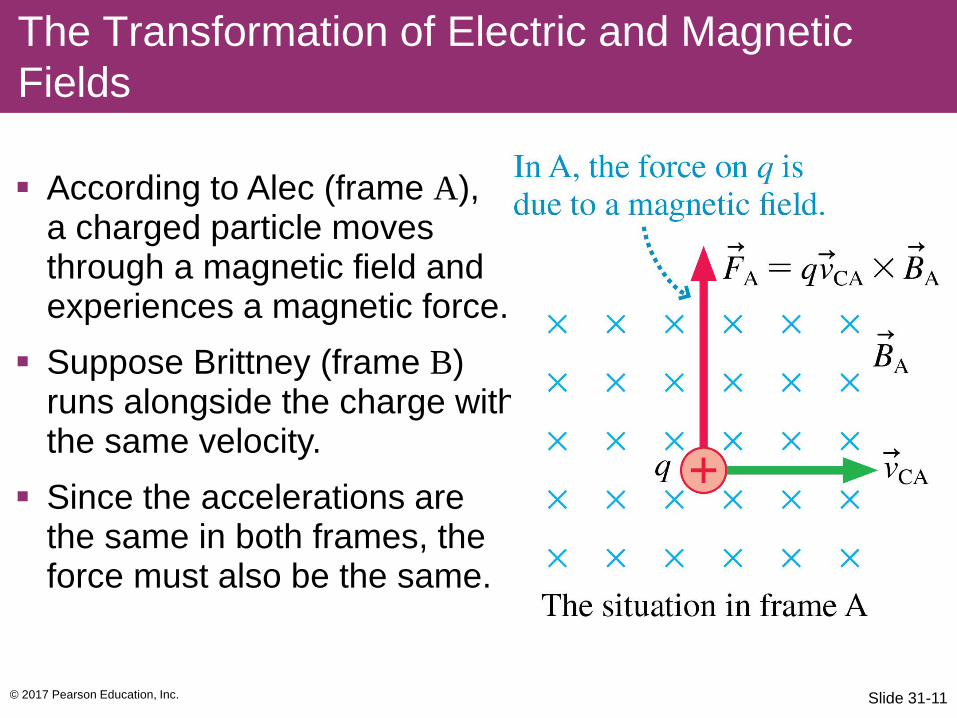
The Transformation of Electric and Magnetic Fields
According to Alec (frame A), a charged particle moves through a magnetic field and experiences a magnetic force.
Suppose Brittney (frame B) runs alongside the charge with the same velocity.
Since the accelerations are the same in both frames, the force must also be the same.
© 2017 Pearson Education, Inc. Slide 31-12
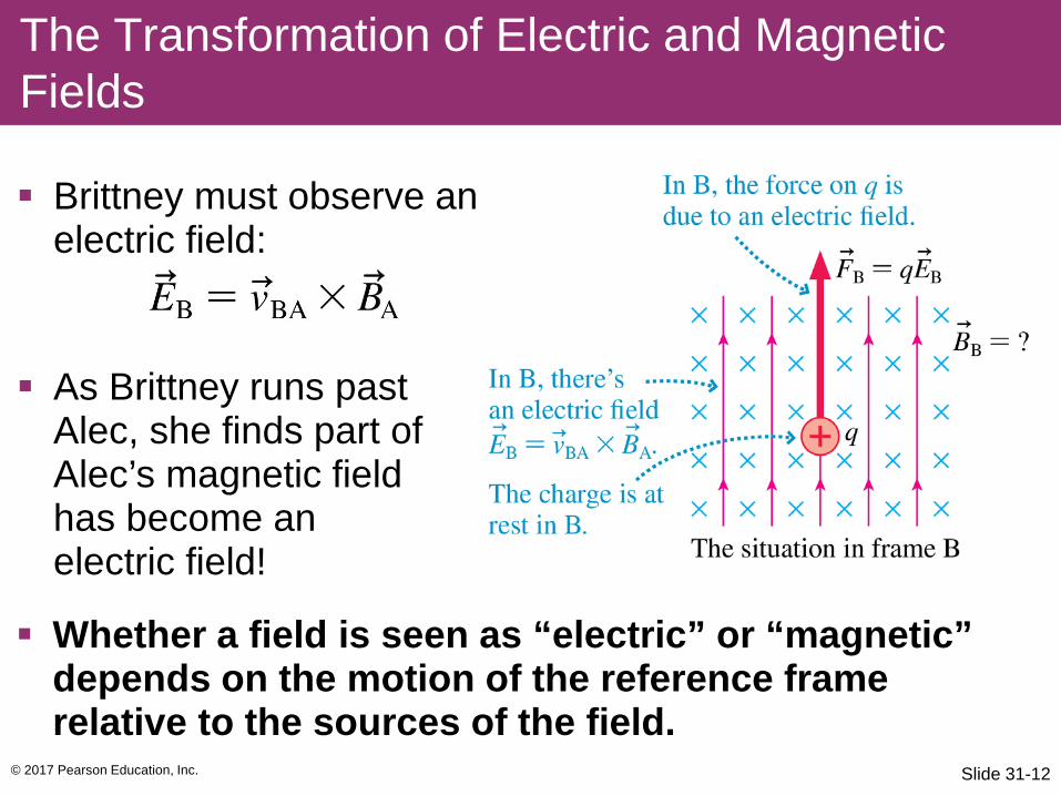
The Transformation of Electric and Magnetic Fields
Brittney must observe an electric field:
As Brittney runs past Alec, she finds part of Alec’s magnetic field has become an electric field!
Whether a field is seen as “electric” or “magnetic” depends on the motion of the reference frame relative to the sources of the field.

© 2017 Pearson Education, Inc. Slide 31-13
The Transformation of Electric and Magnetic Fields
A charge in reference frame A experiences electric and magnetic forces.

© 2017 Pearson Education, Inc. Slide 31-14
The Transformation of Electric and Magnetic Fields
The charge experiences the same force in frame B, but it is due only to an electric field.

© 2017 Pearson Education, Inc. Slide 31-15
Example 31.1 Transforming the Electric Field
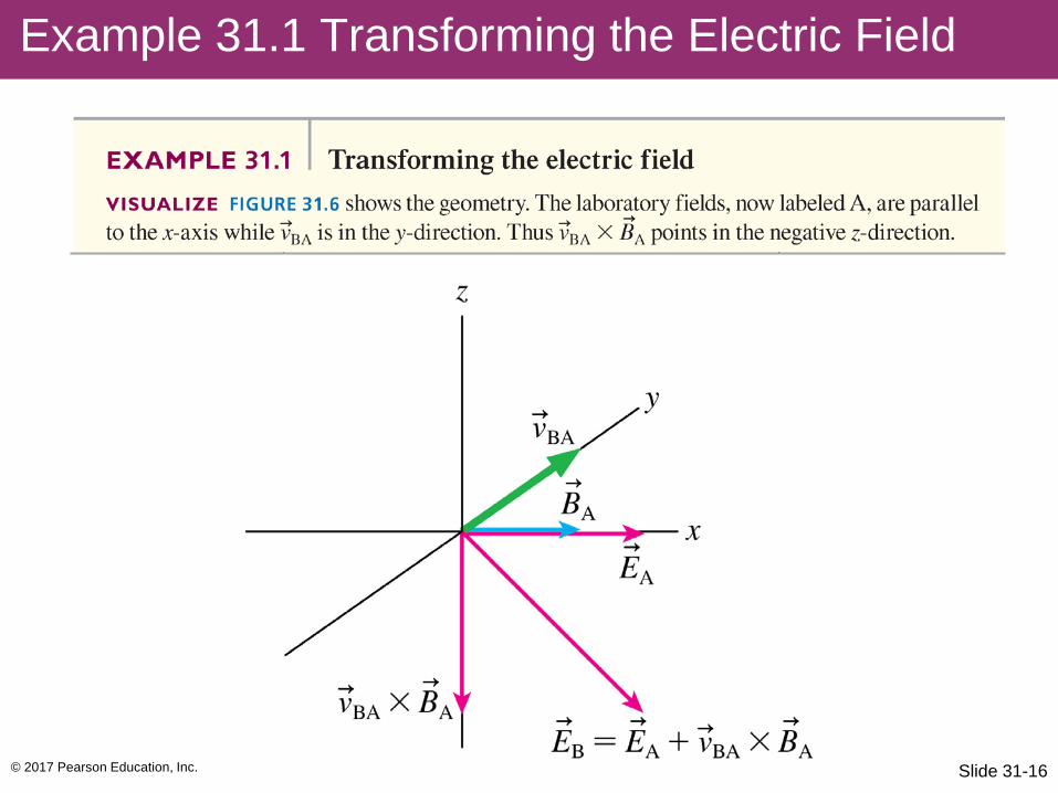
© 2017 Pearson Education, Inc. Slide 31-16
Example 31.1 Transforming the Electric Field

© 2017 Pearson Education, Inc. Slide 31-17
Example 31.1 Transforming the Electric Field

© 2017 Pearson Education, Inc. Slide 31-18
The Transformation of Electric and Magnetic Fields
The Galilean field transformation equations are
where is the velocity of reference frame B relative to frame A.
The fields are measured at the same point in space by experimenters at rest in each reference frame.
These equations are only valid if vBA << c.

© 2017 Pearson Education, Inc. Slide 31-19
Galilean Field Transformation Equations
The figure shows two positive charges moving side by side through frame A.
Charge q2 experiences both an electric and magnetic field due to charge q1.

© 2017 Pearson Education, Inc. Slide 31-20
Galilean Field Transformation Equations
In the reference frame in which the charges are both at rest, charge q1 experiences only an electric field due to charge q2.
The magnitude of the electric field in frame B as predicted by the Galilean field transformation equations is too high by a factor of (1 – vBA
2/c2). When vBA << c, this
difference can be neglected.

© 2017 Pearson Education, Inc. Slide 31-21
Faraday’s Law Revisited
The figure shows a laboratory reference frame A in which a conducting loop is moving into a static magnetic field.
The magnetic field exerts an upward magnetic force on the charges in the leading edge of the wire.
This induces a current in the loop. We call this a motional emf.

© 2017 Pearson Education, Inc. Slide 31-22
Faraday’s Law Revisited
An experimenter in the loop’s frame sees not only a magnetic field but also an electric field, which is what drives the current.
This is the induced electric field of Faraday’s law.
The induced electric field only exists in the loop frame of reference, in which the magnetic field is moving.

© 2017 Pearson Education, Inc. Slide 31-23
The Field Laws Thus Far: 1. Gauss’s Law
Gauss’s law for the electric field says that for any closed surface enclosing total charge Qin, the net electric flux through the surface is
The circle on the integral sign indicates that the integration is over a closed surface.

© 2017 Pearson Education, Inc. Slide 31-24
The Field Laws Thus Far: 2. Gauss’s Law for Magnetic Fields
Magnetic field lines form continuous curves: Every field line leaving a surface at some point must reenter it at another.
Gauss’s law for the magnetic field states that the net magnetic flux through a closed surface is zero:

© 2017 Pearson Education, Inc. Slide 31-25
The Field Laws Thus Far: 3. Faraday’s Law
Faraday’s law states that a changing magnetic flux through a closed loop creates an induced emf around the loop:
Where the line integral of is around the closed curve that bounds the surface through which the magnetic flux is calculated.
This equation means that an electric field can be created by a changing magnetic field.

© 2017 Pearson Education, Inc. Slide 31-26
Ampère’s Law
Ampère’s law states that whenever total current Ithrough passes through an area bounded by a closed curve, the line integral of the magnetic field around the curve is
Ampère’s law is the formal statement that currents create magnetic fields.

© 2017 Pearson Education, Inc. Slide 31-27
Tactics: Determining the Signs of Flux and Current

© 2017 Pearson Education, Inc. Slide 31-28
Ampère’s Law
Ampère’s law may be applied to the current Ithrough passing through any surface S that is bounded by curve C.

© 2017 Pearson Education, Inc. Slide 31-29
Maxwell’s Correction to Ampère’s Law
The figure shows a capacitor being charged.
Curve C is a closed curve encircling the wire on the left.
Surface S1 has Ithrough = I, but surface S2 has Ithrough = 0!
Ampère’s law is either wrong or incomplete.

© 2017 Pearson Education, Inc. Slide 31-30
Maxwell’s Correction to Ampère’s Law
The rate at which the electric flux is changing through surface S2 is
Maxwell added a correction term to Ampère’s law using what he called the displacement current:

© 2017 Pearson Education, Inc. Slide 31-31
The Field Laws Thus Far: 4. The Ampère-Maxwell Law
The Ampère-Maxwell law states that a changing electric flux through a closed loop or an electric current through the loop creates a magnetic field around the loop:
Where the line integral of is around the closed curve that bounds the surface through which the electric flux and current are flowing.
This equation means that a magnetic field can be created either by an electric current or by a changing electric field.

© 2017 Pearson Education, Inc. Slide 31-32
Induced Fields
An increasing solenoid current causes an increasing magnetic field, which induces a circular electric field.
An increasing capacitor charge causes an increasing electric field, which induces a circular magnetic field.

© 2017 Pearson Education, Inc. Slide 31-33
Maxwell’s Equations
Electric and magnetic fields are described by the four Maxwell’s Equations:
© 2017 Pearson Education, Inc. Slide 31-34
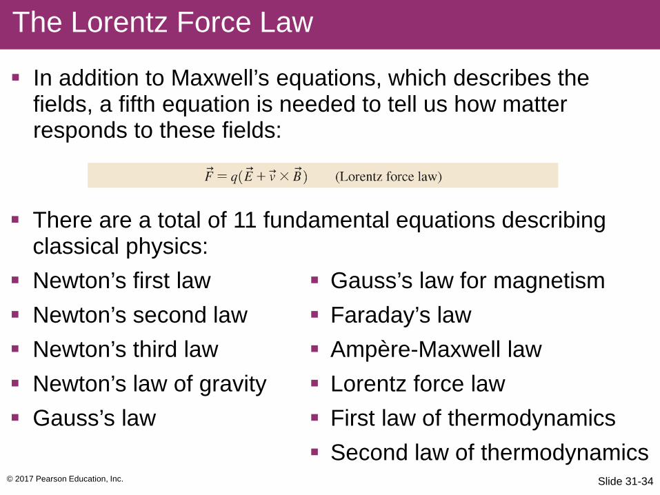
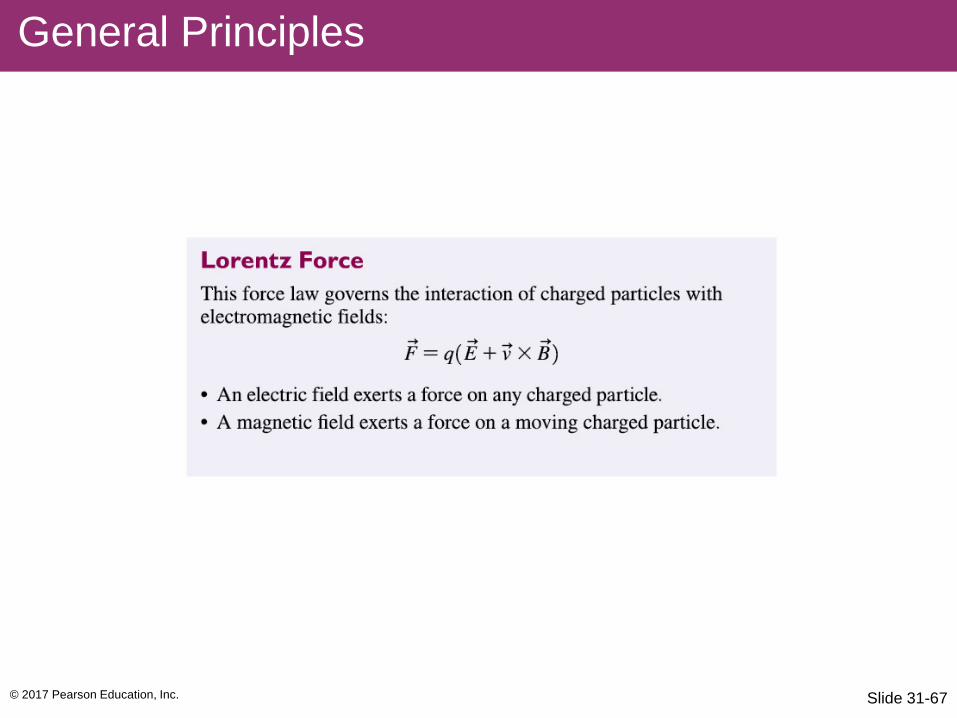
The Lorentz Force Law
In addition to Maxwell’s equations, which describes the fields, a fifth equation is needed to tell us how matter responds to these fields:
There are a total of 11 fundamental equations describing classical physics:
Newton’s first law Newton’s second law Newton’s third law Newton’s law of gravity Gauss’s law
Gauss’s law for magnetism Faraday’s law Ampère-Maxwell law Lorentz force law First law of thermodynamics Second law of thermodynamics

© 2017 Pearson Education, Inc. Slide 31-35
The Fundamental Ideas of Electromagnetism
Let’s summarize the physical meaning of the five electromagnetic equations:

© 2017 Pearson Education, Inc. Slide 31-36
Advanced Topic: Electromagnetic Waves
Maxwell was the first to understand that light is an oscillation of the electromagnetic field.
Maxwell was able to predict that electromagnetic waves can exist at any frequency, not just at the frequencies of visible light.
This prediction was the harbinger of radio waves.
Large radar installations like this one are used to track rockets and missiles.

© 2017 Pearson Education, Inc. Slide 31-37
Advanced Topic: Electromagnetic Waves
Maxwell’s equations lead to a wave equation for the electric and magnetic fields.
The source-free Maxwell’s equations, with no charges or currents, are

© 2017 Pearson Education, Inc. Slide 31-38
Advanced Topic: Electromagnetic Waves
A changing magnetic field creates an induced electric field, and a changing electric field creates an induced magnetic field.
If a changing magnetic field creates an electric field that, in turn, happens to change in just the right way to recreate the original magnetic field, then the fields can exist in a self-sustaining mode.

© 2017 Pearson Education, Inc. Slide 31-39
Advanced Topic: Electromagnetic Waves
This figure shows the fields due to a plane wave, traveling to the right along the x-axis.
The fields are the same everywhere in any yz-plane perpendicular to x.

© 2017 Pearson Education, Inc. Slide 31-40
Advanced Topic: Electromagnetic Waves
This figure shows that the fields—at one instant of time—do change along the x-axis.
These changing fields are the disturbance that is moving down the x-axis at speed vem, so and of a plane wave are functions of the two variables x and t.

© 2017 Pearson Education, Inc. Slide 31-41
Advanced Topic: Electromagnetic Waves
Consider an imaginary box, a Gaussian surface, centered on the x-axis.
There is no charge in the box, and for a plane wave the net electric and magnetic flux through the box is zero, so the plane wave is consistent with the first two of Maxwell’s equations.

© 2017 Pearson Education, Inc. Slide 31-42
Advanced Topic: Faraday’s Law
Let’s apply Faraday’s law to the narrow rectangle in the xy-plane shown.
The magnetic field is perpendicular to the rectangle, so the magnetic flux is Φm= Bz Arectangle = Bzh∆x.
As the wave moves, the flux changes at the rate

© 2017 Pearson Education, Inc. Slide 31-43
Advanced Topic: Faraday’s Law The electric field points in the y-direction; hence at all points
on the top and bottom edges the contribution to the integral is zero.
Along the left edge of the loop, at position x, Ey has the same value at every point.
We can write Faraday’s law as
The area h ∆x of the rectangle cancels, and we’re left with
© 2017 Pearson Education, Inc. Slide 31-44
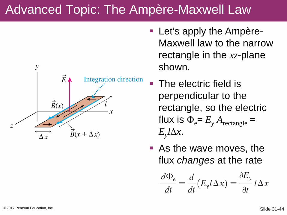
Advanced Topic: The Ampère-Maxwell Law Let’s apply the Ampère-
Maxwell law to the narrow rectangle in the xz-plane shown.
The electric field is perpendicular to the rectangle, so the electric flux is Φe= Ey Arectangle = Eyl∆x.
As the wave moves, the flux changes at the rate

© 2017 Pearson Education, Inc. Slide 31-45
Advanced Topic: The Ampère-Maxwell Law
We can write the Ampère-Maxwell law as
The area of the rectangle cancels, and we’re left with

© 2017 Pearson Education, Inc. Slide 31-46
Advanced Topic: The Wave Equation If we start with the Faraday’s law requirement for any
electromagnetic wave, we can take the second derivative with respect to x, and combine this with the Ampère-Maxwell law requirement to obtain a wave equation
Comparing this with the general wave equation studied in Chapter 16, we see that an electromagnetic wave must travel (in vacuum) with speed

© 2017 Pearson Education, Inc. Slide 31-47
Properties of Electromagnetic Waves
This figure shows the electric and magnetic fields at points along the x-axis, due to a passing electromagnetic wave.
The field strengths are related by E = cB at every point on the wave.

© 2017 Pearson Education, Inc. Slide 31-48
The Poynting Vector
The energy flow of an electromagnetic wave is described by the Poynting vector:
The Poynting vector points in the direction in which an electromagnetic wave is traveling.
The units of S are W/m2; the magnitude S of the Poynting vector measures the instantaneous rate of energy transfer per unit area of the wave.

© 2017 Pearson Education, Inc. Slide 31-49
Intensity of Electromagnetic Waves
The Poynting vector is a function of time, oscillating from zero to Smax = E0
2/cμ0 and back to zero twice during each period of the wave’s oscillation.
Of more interest is the average energy transfer, averaged over one cycle of oscillation, which is the wave’s intensity I.
The intensity of an electromagnetic wave is
The intensity of electromagnetic waves at a distance r away from an isotropic source with power Psource is

© 2017 Pearson Education, Inc. Slide 31-50
Example 31.4 Fields of a Cell Phone

© 2017 Pearson Education, Inc. Slide 31-51
Example 31.4 Fields of a Cell Phone
© 2017 Pearson Education, Inc. Slide 31-52
Example 31.4 Fields of a Cell Phone

© 2017 Pearson Education, Inc. Slide 31-53
Radiation Pressure
Suppose we shine a beam of light on an object that completely absorbs the light energy.
The momentum transfer will exert an average radiation pressure on the surface:
Artist’s conception of a future spacecraft powered by radiation pressure from the sun. where I is the intensity
of the light wave.
Electromagnetic waves transfer not only energy but also momentum.

© 2017 Pearson Education, Inc. Slide 31-54
Example 31.5 Solar Sailing

© 2017 Pearson Education, Inc. Slide 31-55
Example 31.5 Solar Sailing

© 2017 Pearson Education, Inc. Slide 31-56
Generating Electromagnetic Waves
An electric dipole creates an electric field that reverses direction if the dipole charges are switched.
An oscillating dipole can generate an electromagnetic wave.
© 2017 Pearson Education, Inc. Slide 31-57
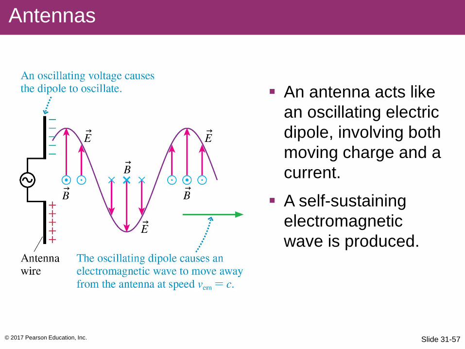
Antennas
An antenna acts like an oscillating electric dipole, involving both moving charge and a current.
A self-sustaining electromagnetic wave is produced.

© 2017 Pearson Education, Inc. Slide 31-58
Polarization
The plane of the electric field vector and the Poynting vector is called the plane of polarization.
The electric field in the figure below oscillates vertically, so this wave is vertically polarized.

© 2017 Pearson Education, Inc. Slide 31-59
Polarization
The electric field in the figure below is horizontally polarized.
Most natural sources of light are unpolarized, emitting waves whose electric fields oscillate randomly with all possible orientations.

© 2017 Pearson Education, Inc. Slide 31-60
Polarization
The most common way of artificially generating polarized visible light is to send unpolarized light through a polarizing filter.
© 2017 Pearson Education, Inc. Slide 31-61
Malus’s Law
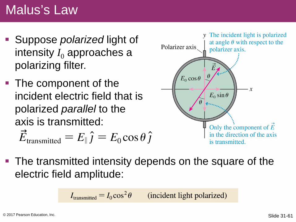
Suppose polarized light of intensity I0 approaches a polarizing filter.
The component of the incident electric field that is polarized parallel to the axis is transmitted:
The transmitted intensity depends on the square of the electric field amplitude:

© 2017 Pearson Education, Inc. Slide 31-62
Polarizers and Analyzers
Malus’s law can be demonstrated with two polarizing filters.
The first, called the polarizer, is used to produce polarized light of intensity I0.
The second, called the analyzer, is rotated by angle θ relative to the polarizer.

© 2017 Pearson Education, Inc. Slide 31-63
Polarizing Filters
The transmission of the analyzer is (ideally) 100% when θ = 0º, and steadily decreases to zero when θ = 90º.
Two polarizing filters with perpendicular axes, called crossed polarizers, block all the light.
If the incident light on a polarizing filter is unpolarized, half the intensity is transmitted:

© 2017 Pearson Education, Inc. Slide 31-64
Polarizing Sunglasses
Glare—the reflection of the sun and the skylight from roads and other horizontal surfaces—has a strong horizontal polarization.
This light is almost completely blocked by a vertical polarizing filter.
Vertically polarizing sunglasses can “cut glare” without affecting the main scene you wish to see.

© 2017 Pearson Education, Inc. Slide 31-65
Chapter 31 Summary Slides

© 2017 Pearson Education, Inc. Slide 31-66
General Principles
© 2017 Pearson Education, Inc. Slide 31-67
General Principles

© 2017 Pearson Education, Inc. Slide 31-68
General Principles

© 2017 Pearson Education, Inc. Slide 31-69
Important Concepts

© 2017 Pearson Education, Inc. Slide 31-70
Important Concepts

© 2017 Pearson Education, Inc. Slide 31-71
Important Concepts

© 2017 Pearson Education, Inc. Slide 31-72
Important Concepts

© 2017 Pearson Education, Inc. Slide 31-73
Applications
Related Documents


