Iowa Storm Water Management Manual Design Standards Chapter 3- Storm Water Hydrology Chapter 3- Section 1 General Information for Stormwater Hydrology Chapter 3- Section 2 Rainfall and Runoff Analysis Chapter 3- Section 3 Time of Concentration Chapter 3- Section 4 Rational Method Chapter 3- Section 5 NRCS TR-55 Methodology Chapter 3- Section 6 Small Storm Hydrology Chapter 3- Section 7 Runoff Hydrograph Determination Chapter 3- Section 8 Low-Impact Development (LID) Hydrology Chapter 3- Section 9 Detention Storage Design Chapter 3- Section 10 Channel and Storage (Reservoir) Routing Chapter 3- Section 11 Inlet Sediment Forebays Chapter 3- Section 12 Detention Basin Outlet Structures Chapter 3- Section 13 Water Balance Calculations Chapter 3- Section 14 Downstream Hydrologic Assessment

Welcome message from author
This document is posted to help you gain knowledge. Please leave a comment to let me know what you think about it! Share it to your friends and learn new things together.
Transcript

Iowa Storm Water Management Manual
Design Standards Chapter 3- Storm Water Hydrology
Chapter 3- Section 1 General Information for Stormwater Hydrology
Chapter 3- Section 2 Rainfall and Runoff Analysis
Chapter 3- Section 3 Time of Concentration
Chapter 3- Section 4 Rational Method
Chapter 3- Section 5 NRCS TR-55 Methodology
Chapter 3- Section 6 Small Storm Hydrology
Chapter 3- Section 7 Runoff Hydrograph Determination
Chapter 3- Section 8 Low-Impact Development (LID) Hydrology
Chapter 3- Section 9 Detention Storage Design
Chapter 3- Section 10 Channel and Storage (Reservoir) Routing
Chapter 3- Section 11 Inlet Sediment Forebays
Chapter 3- Section 12 Detention Basin Outlet Structures
Chapter 3- Section 13 Water Balance Calculations
Chapter 3- Section 14 Downstream Hydrologic Assessment

Page 1 of 5 October 28, 2009
Chapter 3- Section 1 General Information for Stormwater Hydrology
A. Introduction
Urban stormwater hydrology includes the information and procedures for estimating flow peaks, volumes, and time
distributions of stormwater runoff. The analysis of these parameters is fundamental to the design of stormwater
management facilities, such as storm drainage systems for conveyance of surface runoff and structural stormwater
controls for quality and quantity. In the hydrologic analysis of a development site, there are a number of variable factors
that affect the nature of stormwater runoff from the site. Some of the factors that must be considered include:
Rainfall amount and storm distribution
Drainage area size, shape, and orientation
Ground cover and soil type
Slopes of terrain and stream channel(s)
Antecedent moisture condition
Storage potential (floodplains, ponds, wetlands, reservoirs, channels, etc.)
Watershed development potential
Characteristics of the local drainage system
The typical hydrologic processes of interest in urban hydrology are related to:
Precipitation and losses (rainfall abstractions)
Determination of peak flow rate
Determination of total runoff volume
Runoff hydrograph (flow vs. time)
Stream channel hydrograph routing and combining of flows
Reservoir (storage) routing
The practice of urban stormwater hydrology is not an exact science. While the hydrologic processes are well-understood,
the necessary equations and boundary conditions required to solve them are often quite complex. In addition, the required
data is often not available. There are a number of empirical hydrologic methods that can be used to estimate runoff
characteristics for a site or drainage subbasin; the methods presented in this section have been selected to support
hydrologic site analysis for the design methods and procedures included in this manual:
Rational method
NRCS Urban Hydrology for Small Watersheds (TR-55, 1986; WinTR-55, 2003)
US Geological Survey (USGS) regression equations
Small storm hydrology methods (water quality treatment volume – WQv and water quality capture volume
calculations)
Low-impact development (LID) hydrologic methods
Water balance calculations
These methods have been included since the applications are well-documented in urban stormwater hydrology design
practice, and have been verified for accuracy in duplicating local hydrologic estimates for a range of design storms. The
applicable design equations, nomographs, and computer programs are readily available to support the methods.
Table C3-S1- 1 lists the hydrologic methods and circumstances for their use in various analysis and design applications.
Table C3-S1- 2 includes some limitations on the use of several of the methods.
1. The Rational method is recommended for small, highly-impervious drainage areas, such as parking lots and
roadways draining into inlets and gutters:
a. Planning level calculations up to 160 acres.
b. Detailed final design for peak runoff calculations of smaller homogeneous drainage areas of up to 60 acres.
2. The NRCS Urban Hydrology for Small Watersheds (WinTR-55) has wide application for existing and developing
urban watersheds up to 2000 acres.

Iowa Storm Water Management Manual C3-S1 - General Information for Stormwater Hydrology
Page 2 of 5 October 28, 2009
3. The USGS regression equations are recommended for drainage areas with characteristics within the ranges given
for the equations. The USGS equations should be used with caution when there are significant storage areas
within the drainage basin, or where other drainage characteristics indicate that general regression equations might
not be appropriate.
Table C3-S1- 1: Applications of hydrologic methods
Method Rational
method
NRCS
Method
USGS
Equations
Water
Quality
Volume
Water quality volume (WQv)
Channel protection volume (Cpv)
Overbank flood protection (Qp5)
Extreme flood protection (Qf)
Storage facilities
Outlet structures
Gutter flow and inlets
Storm sewer piping
Culverts
Small ditches
Open channels
Energy dissipation
Table C3-S1- 2: Limitations of hydrologic methods
Method Size
Limitations Comments
Rational ≤160 acres Method can be used for estimating peak flows and the design of small site
or subdivision storm sewer systems. Should not be used for storage
design.
NRCS 0-2000 acres Method can be used for estimating peak flows and hydrographs for all
design applications. Can be used for low-impact development hydrologic
analysis.
USGS
regression
Method can be used for estimating peak flows for all design applications.
Water quality Methods used for calculating the water quality volume (WQv):
(1) Simplified method, (2) NRCS CN method, (3) water quality capture
volume method.
B. Definitions
1. Travel time (Tt) and time of concentration (Tc). Travel time is the time it takes for water to travel from one
location to another in a watershed. Tt is a component of the time of concentration, Tc, which is the time for runoff
to travel from the hydraulically most distant point of the watershed to a point of interest within the watershed. Tc
is computed by summing all the travel times for consecutive components of the drainage conveyance system.
2. Infiltration. Infiltration is the process through which precipitation enters the soil surface and moves through the
upper soil profile.
3. Depression storage. Depression storage is the natural depressions within the ground surface and landscape that
Iowa Storm Water Management Manual C3-S1 - General Information for Stormwater Hydrology
Page 3 of 5 October 28, 2009
collect and store rainfall runoff, either temporarily or permanently.
4. Interception. Interception is the storage of rainfall on foliage and other intercepting surfaces, such as vegetated
pervious areas, during a rainfall event.
5. Rainfall excess. After interception, depression storage, and infiltration have been satisfied, rainfall excess is the
remaining water available to produce runoff.
6. Hyetograph. A hyetograph is a graph of the time distribution of rainfall over a watershed (rainfall intensity
(in/hr) or volume vs. time).
7. Hydrograph. A hydrograph is a graph of the time distribution of runoff from a watershed.
8. Unit hydrograph. The hydrograph resulting from 1 inch of rainfall excess generated uniformly over the watershed, at a uniform rate, for a specified period of time. There are several types of unit hydrographs. The use of unit hydrographs to create direct runoff hydrographs is discussed in more detail in Section 2C-7. An example of the NRCS dimensionless unit hydrograph and the relationships to the other components presented above is shown in Figure C3-S1- 1.
9. Peak discharge. The peak discharge (peak flow) is the maximum rate of flow of water passing a given point
during or after a rainfall event (or snowmelt).
10. Runoff volume. The runoff volume represents the volume of rainfall excess generated from the watershed area.
The runoff volume is often expressed in watershed-inches or acre-feet. The runoff volume for a rainfall event can
also be represented by the area under the runoff portion of the hydrograph.
Figure C3-S1- 1: NRCS dimensionless curvilinear unit hydrograph and equivalent triangular hydrograph
C. Concepts
The hydrologic concepts of interest with respect to the design of BMPs are closely related to the design objectives of the
BMP. Design of BMPs can be focused on peak discharge control, volume control, water quality management, pollutant
removal, groundwater recharge, thermal control, or a combination of two or more of these objectives. Each control
objective has somewhat different hydrologic parameter requirements that will need to be addressed in the design of the
BMP to achieve these objectives.

Iowa Storm Water Management Manual C3-S1 - General Information for Stormwater Hydrology
Page 4 of 5 October 28, 2009
The addition of water quality considerations in the design of BMPs adds a new dimension to the hydrologic
considerations for traditional BMP design. Prior to the introduction of water quality considerations, hydrologic design
methods were focused on flood event hydrology focused on storms typically ranging from the 2-year (bank-full), 5-year to
10-year (storm drainage conveyance storm), to the 100-year (floodplain storm). Water quality considerations require a
shift from flood events to annual rainfall volumes and the associated pollutant loads. Concepts such as the rainfall
frequency spectrum and small storm hydrology become important when designing for water quality. These, along with
traditional concepts, are summarized below.
1. Large versus small storm hydrology. Traditional practice in stormwater management has focused on flood
events ranging from the 2-year to the 100-year storm. The increased emphasis on addressing the quality of urban
stormwater has resulted in the realization that small storms (i.e. <1-1.5 inches of rainfall) dominate watershed
hydrologic parameters typically associated with water quality management issues and BMP design. These small
storms are responsible for most annual urban runoff and groundwater recharge. Likewise, with the exception of
eroded sediment, they are responsible for most pollutant wash-off from urban surfaces. Therefore, the small
storms are of most concern for the stormwater management objectives of ground water recharge, water quality
resource protection, and thermal impacts control. Medium storms, defined as storms with a return frequency of 6
months to 2 years, are the dominant storms that determine the size and shape of the receiving streams. These
storms are critical in the design of BMPs that protect stream channels from accelerated erosion and degradation.
For example, the problem with traditional detention BMPs is not the BMPs themselves, but the design guidance
for BMP outlet flow control that usually does not take into account the geomorphologic character of the receiving
stream.
The larger, more infrequent storms have traditionally been used for the design of stormwater conveyance facilities
such as storm sewers and detention basins for peak discharge control; to prevent local overbank flooding on urban
streams and flooding of structures located in the floodplains of stream channels. These storms have a return
frequency of 2-100 years. For traditional urban drainage design, the 2-10-year storm events are termed “minor
storms,” and those with a recurrence interval >10 years are called “major storms.” In this case, minor storms
should not be confused with the concept of small storm hydrologic events as described above. Although the larger
storms may contain significant pollutant loads for a single runoff event, the contribution to the annual average
pollutant load is really quite small due to the infrequency of occurrence. In addition, longer periods of recovery
are available to receiving waters between larger storm events.
Most rainfall events are much smaller than the design storms used for urban drainage models. In any given area,
most frequently recurrent rainfall events are small (less than 1 inch of daily rainfall). Additional details and
procedures are included in Chapter 3, section 2.
A detailed discussion of small storm hydrology is presented in Chapter 3, section 6.
2. Rainfall frequency spectrum. A rainfall frequency spectrum (RFS), defined as the distribution of all rainfall
events (see example in Figure C3-S6- 3), is a useful tool placing in perspective many of the relevant hydrologic
parameters. Represented in this distribution is the rainfall volume from all storm events ranging from the smallest,
most frequent events in any given year; to the largest, most extreme events, such as the 100-year frequency event,
over a long duration.
The RFS consists of classes of frequencies, often broken down by return period ranges. Four principal classes are
typically targeted for control by stormwater management practices. The two smallest, or most frequent, classes are
often referred to as water quality storms, for which the control objectives are groundwater recharge, pollutant load
reduction, and to some extent, control of channel-erosion-producing events. The two larger, or less frequent,
classes are typically referred to as quantity storms, for which the control objectives are channel erosion control,
overbank control, and flood control.
The runoff volume is the most important hydrologic variable for water quality protection and design because
water quality is a function of the capture and treatment of the mass load of pollutants. The runoff peak rate is the
most important hydrologic variable for drainage system design and flooding analysis. Water quality facilities are
designed to treat a specified quantity or volume of runoff for the full duration of a storm event, as opposed to

Iowa Storm Water Management Manual C3-S1 - General Information for Stormwater Hydrology
Page 5 of 5 October 28, 2009
accommodating only an instantaneous peak at the most severe portion of a storm event. To design effective BMPs
and evaluate water quality impacts in urban watersheds, it is necessary to predict the following hydrologic
processes:
Amount and distribution of rainfall volume
Amount of rainfall that contributes to runoff volume, i.e., rainfall volume minus abstractions
D. Methods of runoff estimation
The Rational method (see Chapter 3, section 4) or approved alternatives may be used in both the minor and major storm
runoff computations for relatively uniform basins in land use and topography, which generally have less than 160 acres
(The American Society of Civil Engineers Water Environment Federation, “Design and Construction of Urban Stormwater
Management Systems,” 1992 edition, states that the Rational method is not recommended for drainage areas much larger
than 100-200 acres).
The averaging of the significantly different land uses through the runoff coefficient of the Rational method should be
minimized where possible. For basins that have multiple changes in land use and topography, or are larger than 160 acres,
or both; the design storm runoff should be analyzed by other methods such as unit hydrographs or computer applications.
These basins should be broken down into subbasins of like uniformity and routing methods applied to determine peak
runoff at specified points. For drainage areas less than 160 acres and when routing is needed, the Modified Rational
method is an acceptable method for drainage areas up to 20 acres.
If the Rational method is not used, TR-55, Urban Hydrology for Small Watersheds (NRCS) (see Chapter 3, section 5),
may be used for drainage areas up to 2000 acres. For areas larger than 2000 acres, TR-20 or an approved alternative may
be used. When computer programs are used for design calculation, it is important to understand the assumptions and limits
for the maximum and minimum drainage area or other limits before it is selected.

Page 1 of 11 December 6, 2016
Chapter 3- Section 2 Rainfall and Runoff Analysis
A. Introduction
1. The first step in any hydrologic analysis is an estimation of the rainfall that will fall on the site for a given time
period. The amount of rainfall can be quantified with the following characteristics:
a. Duration (hours). Length of time over which rainfall (storm event) occurs.
b. Depth (inches). Total amount of rainfall occurring during the storm duration.
c. Intensity (inches per hour). Depth divided by the duration.
2. A design event is used as a basis for determining the design of a new urban storm water management project or
evaluating an existing project. It is presumed that the project will function properly if it can accommodate the
design event at full capacity. For economic reasons, some risk of failure is allowed in selection of the design
event. This risk is usually related to return period.
3. The frequency of a rainfall event is the recurrence interval of storms having the same duration and volume
(depth). This can be expressed either in terms of exceedance probability or return period.
a. Exceedance probability. Probability that a storm event having the specified duration and volume will be
exceeded in one given time period, typically one year.
b. Return period. Average length of time between events that have the same duration and volume.
Thus, if a storm event with a specified duration and volume has a 1% chance of occurring in any given year, then it has an
exceedance probability of 0.01, and a return period of 100 years.
Urban stormwater projects are designed based on storm runoff, so a runoff event must be selected for design. However,
runoff data are usually not available to determine the discharge-return period or runoff volume-return period for design.
Rainfall data is available in various formats for a number of gauge stations across Iowa.
Summary data can be accessed at: http://mesonet.agron.iastate.edu/climodat/index.phtml. Hourly (TD3240) and 15-
minute (TD3260) rainfall data are available from the National Climate Data Center: http://www.ncdc.noaa.gov/cdo-
web/search for the National Weather Service Coop recording gauge stations in Iowa. Most all of the Coop stations in Iowa
have a minimum of 60 years of hourly rainfall data, and many have 100 years on record. A rainfall record is converted to
runoff using a rainfall-runoff model. Two methods are available: a continuous simulation approach, and the single-event
design storm approach. For the continuous simulation method, a chronological record of rainfall for the area of interest is
used as input to a rainfall-runoff model of the urban watershed being considered. The output can then be used as a
chronological record of runoff to determine the maximum runoff peak and total volume for a selected design period. The
Storm Water Management Model (SWMM v.5, EPA) and HEC-HMS (Hydraulic Engineering Center, USACE) are
examples of models with continuous simulation capability. Both of these programs are available as public domain
software programs. The software programs define the format for importing the rainfall data.
In the single-event design storm method, a rainfall record is analyzed to obtain a rainfall-return period relationship. Next,
the storm event corresponding to a design return period is identified as the design storm. This design storm is then used as
input to a mathematical rainfall-runoff model (i.e. Rational method, NRCS WinTR-55), and the resulting output is adopted
as the design runoff (peak rate and/or volume). The single-event design storm method is the most commonly-used method
for smaller urban catchments and urban developments. For assessment of larger urban stormwater systems (>1 mi2) and
regional detention basins, a continuous simulation method is recommended.
The design storm can be described as a return period, rainfall depth, average rainfall intensity, rain duration, or a time
distribution of rainfall. Rainfall intensity refers to the time rate of rainfall (in/hr). The intensity will vary over the duration
of the event, and a plot of rainfall intensity vs. time is called a hyetograph. The total depth of rainfall is the depth to which
the rain would accumulate if it stayed in place where it fell. The average intensity is the total rainfall depth divided by the
storm duration. Rain intensity will exhibit spatial variation, but is usually not considered for small urban watersheds
(<2000 acres).
The selection of the return period for design will depend on the relative importance of the facility being designed, cost

Iowa Storm Water Management Manual C3-S2 - Rainfall and Runoff Analysis
Page 2 of 11 December 6, 2016
(economics), desired level of protection, and damages resulting from a failure. Typical design return periods for storm
sewer conveyance in Iowa (inlets and piping) vary from 2-10 years, with 5 years being most common. For culverts, design
periods of 25-50 years are typical, depending on the type and level of service for the roadway. For detention basins, 25-
100 years are common. Additional specific design storm criteria for stormwater quality and quantity management are
covered in later sections of this manual.
The design storm duration also depends on the type of project. For peak discharge design of urban storm sewers and
culverts, the design storm should be the one that results in the largest peak discharge for a given return period. For urban
areas with a mix of pervious and impervious area, as the imperviousness increases, the time of concentration will
decrease, and the peak runoff rate will increase. The shorter Tc will result in a higher rainfall intensity, and will give the
highest peak discharge. As will be covered later in the Rational method for determining peak runoff rate, duration, and
subsequently the rainfall intensity used for input, is dependent on the time of concentration for the catchment
configuration. For storm sewer design, a minimum duration of 5 minutes is typically specified.
For development of runoff hydrographs using unit hydrograph methods, a storm duration much longer than the time of
concentration is selected. For the NRCS methods for unit hydrograph development, the duration of the storm will be
almost twice the time of concentration.
As described later in this manual, the design storm for management of stormwater quality is defined as the rainfall depth
representing the 90% cumulative probability annual rainfall depth – this is the depth of rainfall that represents 90% of the
rainfall events, based on a cumulative occurrence frequency. These will be the rainfall events with a recurrence interval of
3-4 months and generally will be less than 1.25 inches in depth. This water quality design storm is used to determine the
water quality volume (WQv) for sizing stormwater quality BMPs. Additional details are provided in Chapter 3, section 6.
The water quality design storm depth is determined using a cumulative frequency analysis of 24-hour precipitation event
totals for the period of record for a local area. The rainfall events with a depth of less than 0.1 inches are excluded from
the analysis, since these very seldom produce measurable runoff. The individual events are then grouped by depth
intervals of 0.2 inches, and the frequency of depth occurrence tabulated to determine the cumulative rainfall depth
occurrence until all of the rainfall events in the period of record are included. The smaller rainfall events are more
frequent (smaller return period) while the larger storms more infrequent (smaller number) and have a larger return period.
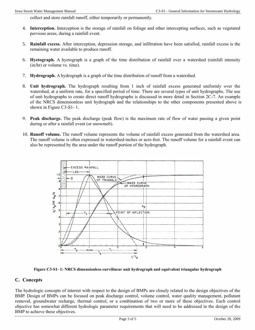
For example, 90% of the annual rainfall events recorded at the NWS Coop rainfall gauge in Ames, Iowa for the period of
record from 1960-2006, are less than or equal to 1.25 inches (computation based only on those rainfall events that
generate measurable runoff; rainfall events less than 0.1 inch were subtracted from the total for calculation of occurrence
frequency. For all rainfall events in the total period of record (100 years for most stations in Iowa), the 90% occurrence
depth is 1 inch or less.
A rainfall analysis for the NWS Coop gauge on the southwest edge of Ames was performed for the period of record 1960-
2006. The results are summarized in Table C3-S2- 1. Rainfall data for all of the NWS Coop sites in Iowa is available from
the National Climate Data Center (NCDC) http://www.ncdc.noaa.gov/cdo-web/search. The data is available in 24-hour
totals recorded at 15-minute and 1-hour intervals. The frequency analysis is completed by first identifying the individual
rainfall events by a separation interval (in this case, 6 hours). This means that each rainfall event is separated from the
next measurable rainfall by the selected interval. The individual rainfall events are then grouped into discrete depth
categories, as shown in the tabulated data for Ames. The number of events in each depth category are totaled, and the
depth class total is divided by the total number of rainfall events for the period of record. For the 1960-2006 period of
record, there were 3,362 events with more than 0.1 inches of precipitation. Rainfall depths less than 0.1 inches usually do
not produce any measurable runoff, so when these events are subtracted from the total, there are 1,999 rainfall events with
greater 0.1 inches depth. The cumulative frequency is computed by dividing the cumulative number of events at each
depth category by the total number of events (1,999) to provide a percent frequency of occurrence for each depth range.
For the Ames data, 90.6% of the rainfall events (greater than 0.1 inch) had a depth of 1.25 inches or less. This is termed
the “90% cumulative occurrence frequency,” and is the rainfall depth recommended for determining the WQv for Iowa.
Also note, for the rainfall frequency for Ames, that the average annual rainfall for the period 1960-2006 was 31.58 inches,
and the mean rainfall depth (P6) is 0.62 inches. The mean rainfall depth, P6, is used in the calculation of the water quality
capture volume (WQCV) for sizing extended detention storage for water quality improvement. The WQv is one of the
unified sizing criteria discussed in Chapter 2 and used throughout this manual for the sizing of stormwater quality BMPs.
The method for WQCV is discussed in more detail in Chapter 3, section 6.
Iowa Storm Water Management Manual C3-S2 - Rainfall and Runoff Analysis
Page 3 of 11 December 6, 2016
Table C3-S2- 1: Rainfall summary for Ames, IA for the period 1960-2006
Rainfall Depth (inches)
Number
of Events
Cumulative
Frequency
Annual Rainfall
in Frequency
Class
Cumulative
Percent of Annual
Average Rainfall
0.01-0.10 1363 2.30
0.11-0.25 651 32.57% 2.98
0.26-0.50 596 62.38% 5.66
0.51-0.75 262 75.49% 4.21
0.76-1.00 182 84.59% 4.08
1.01-1.25 120 90.60% 3.47 69.7%
1.26-1.50 73 94.25% 2.57 78.4%
1.51-1.75 37 96.10% 1.56 83.8%
1.76-2.00 32 97.70% 1.52 89.0%
2.01-3.00 35 99.45% 2.14 96.3%
3.01-4.00 8 99.85% 0.70 98.7%
4.01-5.00 1 99.90% 0.11 99.0%
5.01-6.00 2 100.00% 0.28 100.0%
>6.00 0
Annual Average
Precipitation 31.58
Total Events > 0.01
Total Events > 0.10
Mean Storm
Depth 0.62- inches
B. Rainfall frequency analysis1
In April 2013, the National Oceanic and Atmospheric Administration (NOAA) released “Atlas 14: Precipitation-Frequency
Atlas of the United States, Volume 8.” Volume 8 of this publication covers the Midwestern States, including Iowa, and
supersedes “Bulletin 71: Rainfall Frequency Atlas of the Midwest” (1992) as the most current precipitation data available.
The Atlas 14 results are provided through NOAA’s Precipitation Frequency Data Server
(http://hdsc.nws.noaa.gov/hdsc/pfds/). Based upon user input, the online database generates a precipitation-frequency
estimate (PFE) for an individual location from the historical records of approximately 280 precipitation recording stations
across the State of Iowa.
The location-specific PFE attribute of Atlas 14 means that precipitation-frequency estimates could be generated for each
community or even each individual project, resulting in hundreds or even thousands of PFE’s across Iowa. This situation
would be both inefficient for designers and impractical for reviewers.
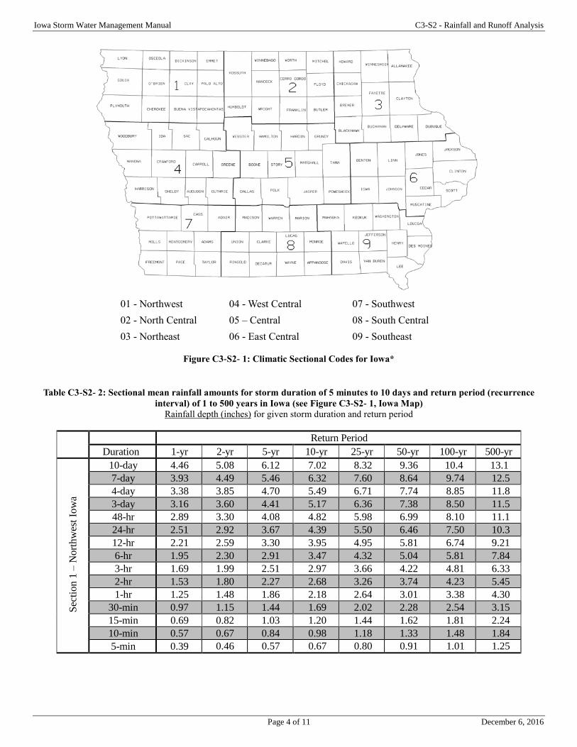
To avoid this dilemma, regional intensity-duration-frequency (IDF) tables corresponding to the nine Iowa climatic sections
in Bulletin 71 were developed. Utilizing Atlas 14, PFE’s were obtained at each county seat. The county values within each
climatic section were then averaged to represent the section as a whole. The resulting IDF values for each climatic section
are provided in Table C3-S2- 2 and Table C3-S2- 3.
1 Adapted from Iowa SUDAS Design Manual, Section 2B-2.
Iowa Storm Water Management Manual C3-S2 - Rainfall and Runoff Analysis
Page 4 of 11 December 6, 2016
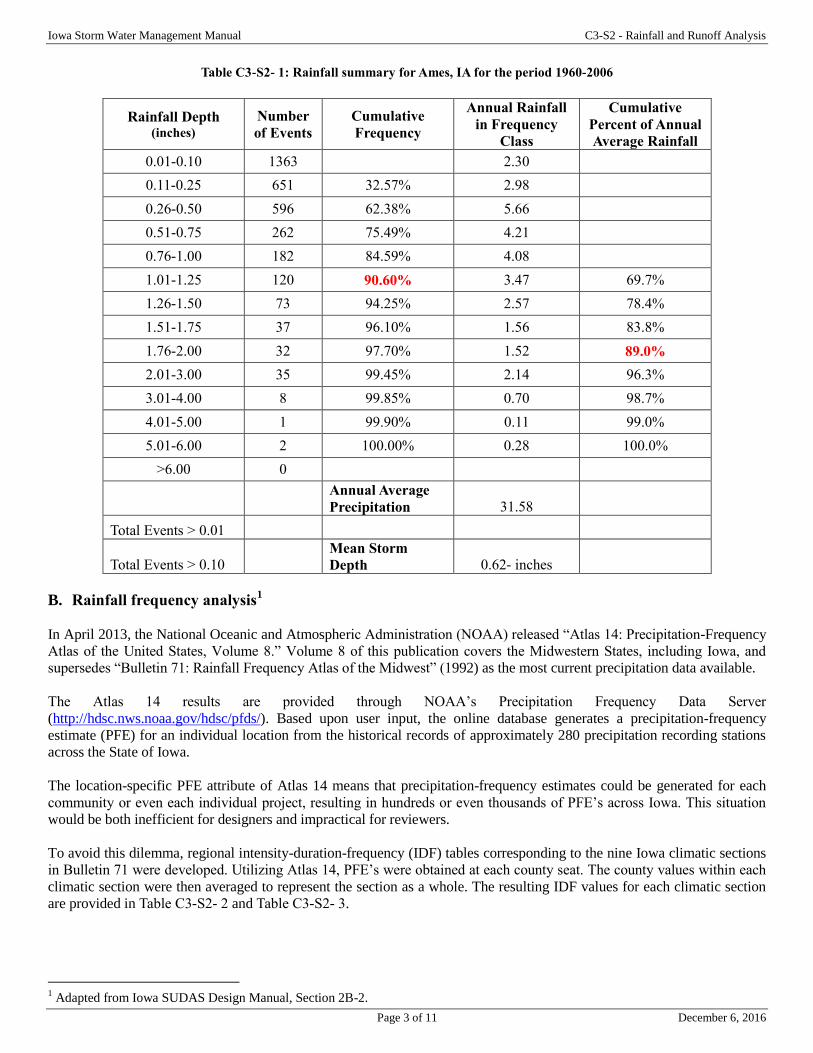
01 - Northwest 04 - West Central 07 - Southwest
02 - North Central 05 – Central 08 - South Central
03 - Northeast 06 - East Central 09 - Southeast
Figure C3-S2- 1: Climatic Sectional Codes for Iowa*
Table C3-S2- 2: Sectional mean rainfall amounts for storm duration of 5 minutes to 10 days and return period (recurrence
interval) of 1 to 500 years in Iowa (see Figure C3-S2- 1, Iowa Map) Rainfall depth (inches) for given storm duration and return period
Return Period
Duration 1-yr 2-yr 5-yr 10-yr 25-yr 50-yr 100-yr 500-yr
Sec
tio
n 1
– N
ort
hw
est
Iow
a
10-day 4.46 5.08 6.12 7.02 8.32 9.36 10.4 13.1
7-day 3.93 4.49 5.46 6.32 7.60 8.64 9.74 12.5
4-day 3.38 3.85 4.70 5.49 6.71 7.74 8.85 11.8
3-day 3.16 3.60 4.41 5.17 6.36 7.38 8.50 11.5
48-hr 2.89 3.30 4.08 4.82 5.98 6.99 8.10 11.1
24-hr 2.51 2.92 3.67 4.39 5.50 6.46 7.50 10.3
12-hr 2.21 2.59 3.30 3.95 4.95 5.81 6.74 9.21
6-hr 1.95 2.30 2.91 3.47 4.32 5.04 5.81 7.84
3-hr 1.69 1.99 2.51 2.97 3.66 4.22 4.81 6.33
2-hr 1.53 1.80 2.27 2.68 3.26 3.74 4.23 5.45
1-hr 1.25 1.48 1.86 2.18 2.64 3.01 3.38 4.30
30-min 0.97 1.15 1.44 1.69 2.02 2.28 2.54 3.15
15-min 0.69 0.82 1.03 1.20 1.44 1.62 1.81 2.24
10-min 0.57 0.67 0.84 0.98 1.18 1.33 1.48 1.84
5-min 0.39 0.46 0.57 0.67 0.80 0.91 1.01 1.25
Iowa Storm Water Management Manual C3-S2 - Rainfall and Runoff Analysis
Page 5 of 11 December 6, 2016
Return Period
Duration 1-yr 2-yr 5-yr 10-yr 25-yr 50-yr 100-yr 500-yr
Sec
tio
n 2
– N
ort
h C
entr
al I
ow
a 10-day 4.78 5.45 6.58 7.56 8.99 10.1 11.3 14.3
7-day 4.19 4.79 5.83 6.76 8.12 9.24 10.1 13.4
4-day 3.55 4.06 4.97 5.80 7.06 8.12 9.26 12.2
3-day 3.31 3.78 4.63 5.42 6.64 7.68 8.80 11.8
48-hr 3.04 3.46 4.26 5.01 6.18 7.19 8.29 11.2
24-hr 2.65 3.06 3.83 4.55 5.67 6.63 7.68 10.4
12-hr 2.34 2.74 3.46 4.14 5.18 6.07 7.03 9.59
6-hr 2.06 2.42 3.07 3.6 4.60 5.38 6.22 8.45
3-hr 1.76 2.08 2.64 3.15 3.91 4.56 5.24 7.04
2-hr 1.58 1.87 2.37 2.82 3.49 4.04 4.63 6.14
1-hr 1.28 1.52 1.92 2.27 2.80 3.23 3.69 4.85
30-min 0.99 1.16 1.47 1.73 2.11 2.42 2.75 3.56
15-min 0.69 0.82 1.03 1.21 1.48 1.69 1.92 2.48
10-min 0.57 0.67 0.84 0.99 1.21 1.39 1.57 2.03
5-min 0.39 0.46 0.57 0.68 0.83 0.95 1.07 1.39
Sec
tion 3
– N
ort
hea
st I
ow
a
10-day 4.76 5.38 6.45 7.39 8.77 9.90 11.0 14.0
7-day 4.17 4.72 5.70 6.58 7.87 8.95 10.1 13.0
4-day 3.53 4.00 4.85 5.64 6.84 7.86 8.95 11.8
3-day 3.28 3.73 4.56 5.32 6.49 7.48 8.56 11.4
48-hr 3.00 3.44 4.23 4.98 6.12 7.10 8.15 10.9
24-hr 2.63 3.04 3.78 4.48 5.56 6.48 7.48 10.1
12-hr 2.32 2.69 3.38 4.02 5.02 5.86 6.79 9.25
6-hr 2.01 2.36 2.98 3.56 4.43 5.17 5.97 8.07
3-hr 1.71 2.01 2.55 3.03 3.74 4.32 4.94 6.55
2-hr 1.53 1.81 2.28 2.70 3.30 3.79 4.30 5.58
1-hr 1.25 1.47 1.85 2.17 2.64 3.01 3.39 4.34
30-min 0.96 1.14 1.41 1.65 1.98 2.23 2.49 3.10
15-min 0.69 0.81 1.00 1.17 1.40 1.57 1.75 2.19
10-min 0.56 0.66 0.82 0.96 1.14 1.29 1.44 1.79
5-min 0.38 0.45 0.56 0.65 0.78 0.88 0.98 1.22
Sec
tion 4
– W
est
Cen
tral
Iow
a
10-day 4.67 5.30 6.38 7.32 8.69 9.80 10.9 13.8
7-day 4.11 4.67 5.66 6.55 7.86 8.94 10.0 13.0
4-day 3.50 3.98 4.86 5.68 6.93 8.00 9.15 12.2
3-day 3.26 3.71 4.56 5.35 6.58 7.63 8.78 11.8
48-hr 2.99 3.41 4.21 4.96 6.16 7.19 8.33 11.4
24-hr 2.63 3.01 3.74 4.45 5.59 6.58 7.67 10.6
12-hr 2.30 2.68 3.39 4.08 5.17 6.12 7.17 10.0
6-hr 2.01 2.36 3.03 3.67 4.69 5.58 6.57 9.24
3-hr 1.71 2.03 2.61 3.16 4.02 4.75 5.55 7.69
2-hr 1.53 1.82 2.35 2.83 3.55 4.17 4.83 6.57
1-hr 1.24 1.48 1.89 2.26 2.81 3.28 3.77 5.05
30-min 0.95 1.13 1.43 1.69 2.08 2.39 2.71 3.53
15-min 0.66 0.78 0.99 1.17 1.43 1.64 1.86 2.42
10-min 0.54 0.64 0.81 0.96 1.17 1.34 1.53 1.98
5-min 0.37 0.44 0.55 0.65 0.80 0.92 1.04 1.35
Iowa Storm Water Management Manual C3-S2 - Rainfall and Runoff Analysis
Page 6 of 11 December 6, 2016
Return Period
Duration 1-yr 2-yr 5-yr 10-yr 25-yr 50-yr 100-yr 500-yr
Sec
tio
n 5
– C
entr
al I
ow
a 10-day 4.87 5.50 6.58 7.52 8.86 9.94 11.0 13.8
7-day 4.25 4.83 5.82 6.69 7.93 8.93 9.98 12.5
4-day 3.59 4.09 4.96 5.74 6.86 7.78 8.74 11.1
3-day 3.34 3.81 4.63 5.36 6.43 7.31 8.25 10.6
48-hr 3.06 3.49 4.25 4.94 5.96 6.81 7.71 10.0
24-hr 2.67 3.08 3.81 4.46 5.44 6.26 7.12 9.37
12-hr 2.34 2.74 3.44 4.07 5.01 5.79 6.62 8.79
6-hr 2.05 2.40 3.03 3.61 4.47 5.20 5.98 8.02
3-hr 1.75 2.06 2.60 3.09 3.82 4.42 5.07 6.76
2-hr 1.58 1.85 2.33 2.76 3.39 3.91 4.46 5.88
1-hr 1.29 1.51 1.89 2.23 2.72 3.13 3.55 4.62
30-min 0.99 1.16 1.45 1.70 2.05 234 2.63 3.36
15-min 0.71 0.83 1.03 1.20 1.45 1.65 1.86 2.37
10-min 0.58 0.68 0.84 0.98 1.19 1.35 1.52 1.94
5-min 0.39 0.46 0.57 0.67 0.81 0.92 1.04 1.33
Sec
tion 6
– E
ast
Cen
tral
Iow
a
10-day 4.75 5.30 6.24 7.04 8.20 9.12 10.0 12.4
7-day 4.17 4.67 5.53 6.29 7.39 8.30 9.25 11.6
4-day 3.53 3.98 4.78 5.50 6.58 7.49 8.46 10.9
3-day 3.28 3.72 4.51 5.24 6.32 7.22 8.19 10.7
48-hr 2.98 3.43 4.22 4.93 6.01 6.90 7.86 10.3
24-hr 2.60 3.01 3.75 4.42 5.44 6.29 7.22 9.64
12-hr 2.28 2.65 3.31 3.93 4.88 5.68 6.56 8.87
6-hr 1.97 2.30 2.89 3.45 4.30 5.02 5.80 7.87
3-hr 1.68 1.96 2.47 2.93 3.63 4.22 4.85 6.50
2-hr 1.51 1.77 2.22 2.62 3.22 3.71 4.24 5.60
1-hr 1.23 1.44 1.80 2.11 2.58 2.96 3.36 4.37
30-min 0.95 1.11 1.38 1.61 1.94 2.20 2.47 3.14
15-min 0.67 0.78 0.97 1.13 1.36 1.54 1.73 2.20
10-min 0.55 0.64 0.80 0.93 1.11 1.26 1.42 1.80
5-min 0.38 0.44 0.54 0.63 0.76 0.86 0.97 1.23
Sec
tion 7
– S
ou
thw
est
Iow
a
10-day 4.95 5.60 6.74 7.75 9.26 10.5 11.8 15.2
7-day 4.35 4.94 5.98 6.93 8.35 9.54 10.8 14.0
4-day 3.67 4.21 5.19 6.08 7.43 8.57 9.79 12.9
3-day 3.41 3.93 4.87 5.73 7.05 8.16 9.36 12.5
48-hr 3.13 3.60 4.47 5.29 6.55 7.62 8.79 11.9
24-hr 2.76 3.18 3.95 4.70 5.86 6.88 7.99 11.0
12-hr 2.42 2.81 3.56 4.27 5.38 6.36 7.42 10.3
6-hr 2.09 2.46 3.15 3.82 4.87 5.78 6.78 9.49
3-hr 1.76 2.10 2.71 3.28 4.16 4.90 5.71 7.86
2-hr 1.58 1.88 2.43 2.92 3.66 4.29 4.95 6.68
1-hr 1.27 1.52 1.95 2.33 2.90 3.36 3.85 5.11
30-min 0.97 1.16 1.47 1.75 2.13 2.44 2.76 3.53
15-min 0.68 0.80 1.02 1.20 1.46 1.67 1.89 2.43
10-min 0.55 0.66 0.83 0.98 1.20 1.37 1.55 1.99
5-min 0.38 0.45 0.57 0.67 0.82 0.93 1.05 1.36
Iowa Storm Water Management Manual C3-S2 - Rainfall and Runoff Analysis
Page 7 of 11 December 6, 2016
Return Period
Duration 1-yr 2-yr 5-yr 10-yr 25-yr 50-yr 100-yr 500-yr
Sec
tio
n 8
– S
ou
th C
entr
al I
ow
a 10-day 5.07 5.73 6.85 7.84 9.27 10.4 11.6 14.7
7-day 4.43 5.04 6.09 7.01 8.38 9.49 10.6 13.6
4-day 3.73 4.29 5.26 6.13 7.43 8.51 9.65 12.6
3-day 3.47 3.99 4.91 5.75 7.01 8.07 9.21 12.1
48-hr 3.18 3.64 4.49 5.28 6.50 7.54 8.66 11.6
24-hr 2.77 3.20 3.99 4.74 5.90 6.90 7.98 10.8
12-hr 2.44 2.81 3.53 4.21 5.29 6.24 7.28 10.1
6-hr 2.15 2.45 3.05 3.64 4.60 5.45 6.40 9.04
3-hr 1.82 2.08 2.59 3.08 3.88 4.58 5.35 7.49
2-hr 1.62 1.86 2.32 2.76 3.45 4.04 4.69 6.45
1-hr 1.29 1.51 1.45 1.71 2.10 2.41 2.75 3.59
30-min 0.98 1.15 1.45 1.71 2.10 2.41 2.75 3.59
15-min 0.69 0.80 1.01 1.19 1.46 1.68 1.91 2.49
10-min 0.56 0.66 0.83 0.98 1.19 1.38 1.56 2.04
5-min 0.38 0.45 0.56 0.67 0.81 0.94 1.07 1.39
Sec
tion 9
– S
outh
east
Iow
a
10-day 4.95 5.54 6.54 7.38 8.57 9.51 10.4 12.8
7-day 4.33 4.87 5.79 6.59 7.72 8.63 9.57 11.8
4-day 3.66 4.16 5.02 5.78 6.88 7.78 8.72 11.0
3-day 3.41 3.90 4.73 5.47 6.56 7.45 8.39 10.7
48-hr 3.12 3.58 4.39 5.11 6.18 7.06 7.98 10.3
24-hr 2.68 3.12 3.90 4.59 5.62 6.46 7.35 9.64
12-hr 2.31 2.71 3.41 4.03 4.96 5.74 6.56 8.68
6-hr 1.99 2.32 2.91 3.44 4.25 4.92 5.63 7.50
3-hr 1.68 1.96 2.45 2.89 3.54 4.08 4.66 6.15
2-hr 1.51 1.76 2.19 2.58 3.14 3.61 4.10 5.35
1-hr 1.23 1.43 1.78 2.09 2.54 2.90 3.28 4.24
30-min 0.95 1.11 1.38 1.61 1.94 2.20 2.46 3.12
15-min 0.68 0.79 0.98 1.14 1.37 1.55 1.74 2.21
10-min 0.55 0.65 0.80 0.93 1.12 1.27 1.43 1.81
5-min 0.38 0.44 0.54 0.64 0.76 0.87 0.97 1.24
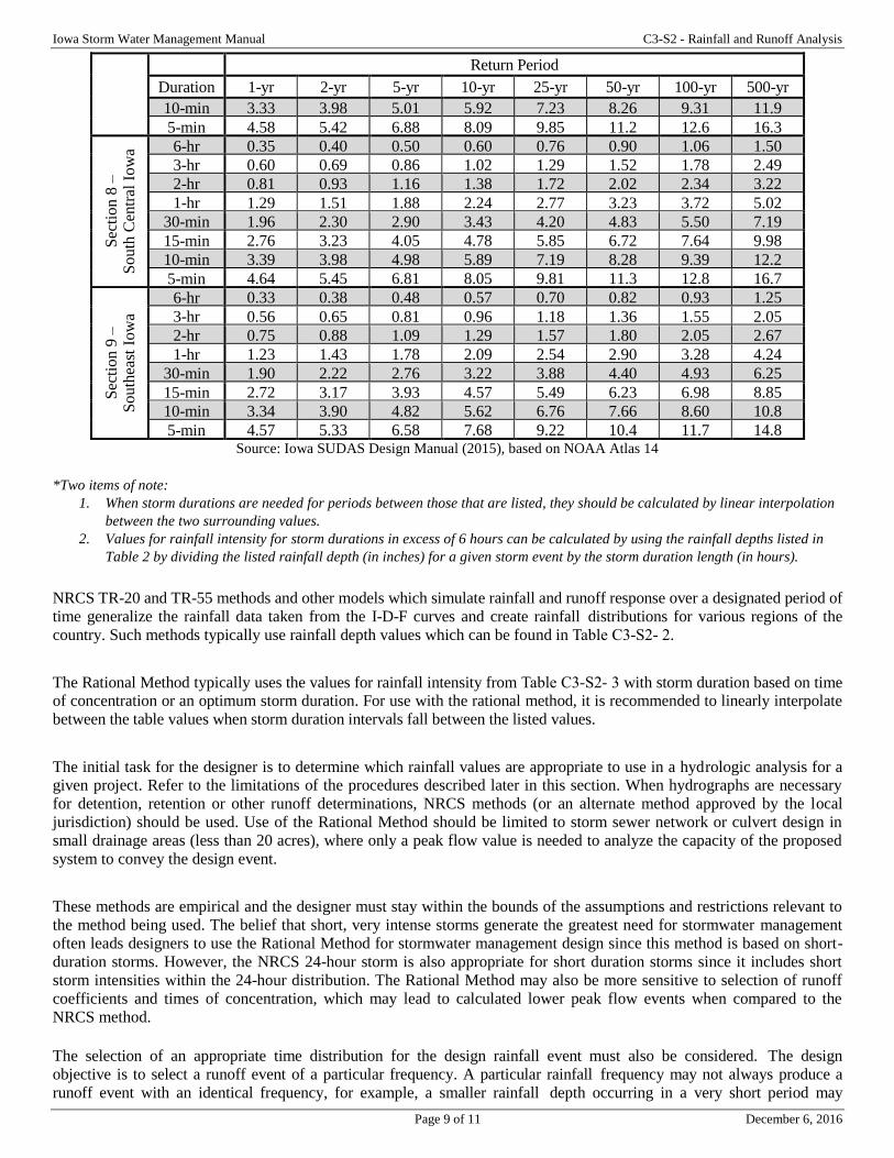
Source: Iowa SUDAS Design Manual (2015), based on NOAA Atlas 14
Table C3-S2- 3: Sectional mean rainfall intensity for storm periods of 5 minutes to 6 hours and return period (recurrence
interval) of 1 to 500 years in Iowa (see Figure C3-S2- 1, Iowa Map)
Rainfall intensity (inches/hour) for given duration and return period
Return Period
Duration 1-yr 2-yr 5-yr 10-yr 25-yr 50-yr 100-yr 500-yr
Sec
tion 1
–
Nort
hw
est
Iow
a
6-hr 0.32 0.38 0.48 0.57 0.72 0.84 0.96 1.30
3-hr 0.56 0.66 0.83 0.99 1.22 1.40 1.60 2.11
2-hr 0.76 0.90 1.13 1.34 1.63 1.87 2.11 2.72
1-hr 1.25 1.48 1.86 2.18 2.64 3.01 3.38 4.30
30-min 1.94 2.30 2.89 3.38 4.05 4.56 5.08 6.30
15-min 2.78 3.29 4.12 4.82 5.77 6.50 7.24 8.98
10-min 3.43 4.06 5.07 5.92 7.09 8.00 8.91 11.0
Iowa Storm Water Management Manual C3-S2 - Rainfall and Runoff Analysis
Page 8 of 11 December 6, 2016
Return Period
Duration 1-yr 2-yr 5-yr 10-yr 25-yr 50-yr 100-yr 500-yr
5-min 4.69 5.53 6.92 8.11 9.69 10.9 12.1 15.0 S
ecti
on
2 –
N
ort
h C
entr
al I
ow
a 6-hr 0.34 0.40 0.51 0.61 0.76 0.89 1.03 1.40
3-hr 0.58 0.69 0.88 1.05 1.30 1.52 1.74 2.34
2-hr 0.79 0.93 1.18 1.41 1.74 2.02 2.31 3.07
1-hr 1.28 1.52 1.92 2.27 2.80 3.23 3.69 4.85
30-min 1.98 2.33 2.94 3.47 4.23 4.85 5.50 7.13
15-min 2.79 3.28 4.12 4.87 5.92 6.79 7.68 9.93
10-min 3.44 4.04 5.07 5.98 7.29 8.35 9.45 12.2
5-min 4.69 5.53 6.93 8.18 9.96 11.4 12.9 16.6
Sec
tio
n 3
–
Nort
hea
st I
ow
a
6-hr 0.33 0.39 0.49 0.59 0.73 0.86 0.99 1.34
3-hr 0.57 0.67 0.85 1.01 1.24 1.44 1.64 2.18
2-hr 0.76 0.90 1.14 1.35 1.65 1.89 2.15 2.79
1-hr 1.25 1.47 1.85 2.17 2.64 3.01 3.39 4.34
30-min 1.93 2.28 2.83 3.31 3.96 4.47 4.98 6.20
15-min 2.77 3.24 4.02 4.68 5.60 6.31 7.03 8.77
10-min 3.40 4.00 4.94 5.76 6.89 7.75 8.64 10.7
5-min 4.66 5.47 6.76 7.86 9.42 10.5 11.8 14.7
Sec
tion 4
–
Wes
t C
entr
al I
ow
a
6-hr 0.33 0.39 0.50 0.61 0.78 0.93 1.09 1.54
3-hr 0.57 0.67 0.87 1.05 1.34 1.58 1.85 2.56
2-hr 0.76 0.91 1.17 1.41 1.77 2.08 2.41 3.28
1-hr 1.24 1.48 1.89 2.26 2.81 3.28 3.77 5.05
30-min 1.91 2.26 2.87 3.39 4.16 4.78 5.42 7.06
15-min 2.66 3.14 3.96 4.69 5.74 6.58 7.46 9.68
10-min 3.29 3.86 4.88 5.76 7.05 8.09 9.18 11.9
5-min 4.47 5.30 6.67 7.88 9.63 11.0 12.5 16.2
Sec
tion 5
–
Cen
tral
Iow
a
6-hr 0.34 0.40 0.50 0.60 0.74 0.86 0.99 1.33
3-hr 0.58 0.68 0.86 1.03 1.27 1.47 1.69 2.25
2-hr 0.79 0.92 1.16 1.38 1.69 1.95 2.23 2.94
1-hr 1.29 1.51 1.89 2.23 2.72 3.13 3.55 4.62
30-min 1.99 2.33 2.91 3.40 4.11 4.68 5.27 6.73
15-min 2.84 3.32 4.12 4.82 5.81 6.61 7.44 9.50
10-min 3.51 4.08 5.08 5.92 7.16 8.13 9.15 11.6
5-min 4.78 5.59 6.91 8.10 9.76 11.1 12.4 15.9
Sec
tio
n 6
–
Eas
t C
entr
al I
ow
a
6-hr 0.32 0.38 0.48 0.57 0.71 0.83 0.96 1.31
3-hr 0.56 0.65 0.82 0.97 1.21 1.40 1.61 2.16
2-hr 0.75 0.88 1.11 1.31 1.61 1.85 2.12 2.80
1-hr 1.23 1.44 1.80 2.11 2.58 2.96 3.36 4.37
30-min 1.90 2.22 2.76 3.22 3.88 4.40 4.95 6.29
15-min 2.70 3.14 3.88 4.53 5.45 6.18 6.94 8.81
10-min 3.33 3.87 4.80 5.58 6.70 7.60 8.54 10.8
5-min 4.56 5.30 6.56 7.65 9.18 10.3 11.6 14.8
Sec
tion 7
–
So
uth
wes
t Io
wa 6-hr 0.34 0.41 0.52 0.63 0.81 0.96 1.13 1.58
3-hr 0.58 0.70 0.90 1.09 1.38 1.63 1.90 2.62
2-hr 0.79 0.94 1.21 1.46 1.83 2.14 2.47 3.34
1-hr 1.27 1.52 1.95 2.33 2.90 3.36 3.85 5.11
30-min 1.94 2.32 2.95 3.50 4.27 4.88 5.52 7.07
15-min 2.72 3.22 4.08 4.82 5.87 6.70 7.57 9.72
Iowa Storm Water Management Manual C3-S2 - Rainfall and Runoff Analysis
Page 9 of 11 December 6, 2016
Return Period
Duration 1-yr 2-yr 5-yr 10-yr 25-yr 50-yr 100-yr 500-yr
10-min 3.33 3.98 5.01 5.92 7.23 8.26 9.31 11.9
5-min 4.58 5.42 6.88 8.09 9.85 11.2 12.6 16.3
Sec
tio
n 8
–
So
uth
Cen
tral
Io
wa 6-hr 0.35 0.40 0.50 0.60 0.76 0.90 1.06 1.50
3-hr 0.60 0.69 0.86 1.02 1.29 1.52 1.78 2.49
2-hr 0.81 0.93 1.16 1.38 1.72 2.02 2.34 3.22
1-hr 1.29 1.51 1.88 2.24 2.77 3.23 3.72 5.02
30-min 1.96 2.30 2.90 3.43 4.20 4.83 5.50 7.19
15-min 2.76 3.23 4.05 4.78 5.85 6.72 7.64 9.98
10-min 3.39 3.98 4.98 5.89 7.19 8.28 9.39 12.2
5-min 4.64 5.45 6.81 8.05 9.81 11.3 12.8 16.7
Sec
tio
n 9
–
So
uth
east
Io
wa
6-hr 0.33 0.38 0.48 0.57 0.70 0.82 0.93 1.25
3-hr 0.56 0.65 0.81 0.96 1.18 1.36 1.55 2.05
2-hr 0.75 0.88 1.09 1.29 1.57 1.80 2.05 2.67
1-hr 1.23 1.43 1.78 2.09 2.54 2.90 3.28 4.24
30-min 1.90 2.22 2.76 3.22 3.88 4.40 4.93 6.25
15-min 2.72 3.17 3.93 4.57 5.49 6.23 6.98 8.85
10-min 3.34 3.90 4.82 5.62 6.76 7.66 8.60 10.8
5-min 4.57 5.33 6.58 7.68 9.22 10.4 11.7 14.8 Source: Iowa SUDAS Design Manual (2015), based on NOAA Atlas 14
*Two items of note:
1. When storm durations are needed for periods between those that are listed, they should be calculated by linear interpolation
between the two surrounding values.
2. Values for rainfall intensity for storm durations in excess of 6 hours can be calculated by using the rainfall depths listed in
Table 2 by dividing the listed rainfall depth (in inches) for a given storm event by the storm duration length (in hours).
NRCS TR-20 and TR-55 methods and other models which simulate rainfall and runoff response over a designated period of
time generalize the rainfall data taken from the I-D-F curves and create rainfall distributions for various regions of the
country. Such methods typically use rainfall depth values which can be found in Table C3-S2- 2.
The Rational Method typically uses the values for rainfall intensity from Table C3-S2- 3 with storm duration based on time of concentration or an optimum storm duration. For use with the rational method, it is recommended to linearly interpolate
between the table values when storm duration intervals fall between the listed values.
The initial task for the designer is to determine which rainfall values are appropriate to use in a hydrologic analysis for a given project. Refer to the limitations of the procedures described later in this section. When hydrographs are necessary
for detention, retention or other runoff determinations, NRCS methods (or an alternate method approved by the local
jurisdiction) should be used. Use of the Rational Method should be limited to storm sewer network or culvert design in
small drainage areas (less than 20 acres), where only a peak flow value is needed to analyze the capacity of the proposed
system to convey the design event.
These methods are empirical and the designer must stay within the bounds of the assumptions and restrictions relevant to
the method being used. The belief that short, very intense storms generate the greatest need for stormwater management
often leads designers to use the Rational Method for stormwater management design since this method is based on short-
duration storms. However, the NRCS 24-hour storm is also appropriate for short duration storms since it includes short
storm intensities within the 24-hour distribution. The Rational Method may also be more sensitive to selection of runoff
coefficients and times of concentration, which may lead to calculated lower peak flow events when compared to the
NRCS method.
The selection of an appropriate time distribution for the design rainfall event must also be considered. The design
objective is to select a runoff event of a particular frequency. A particular rainfall frequency may not always produce a
runoff event with an identical frequency, for example, a smaller rainfall depth occurring in a very short period may

Iowa Storm Water Management Manual C3-S2 - Rainfall and Runoff Analysis
Page 10 of 11 December 6, 2016
actually produce a larger peak runoff than a larger rainfall event spread more uniformly over the event duration. As the
size of the watershed decreases and the imperviousness increases, the selection of the distribution becomes critical. Larger
and less impervious watersheds will often attenuate the large pulses of rainfall and smooth out the runoff hydrographs.
This rainfall distribution criterion is inherent in the governing assumption in the Rational Method that the duration be
equal to the time of concentration, and the watershed be fairly homogeneous in land use.
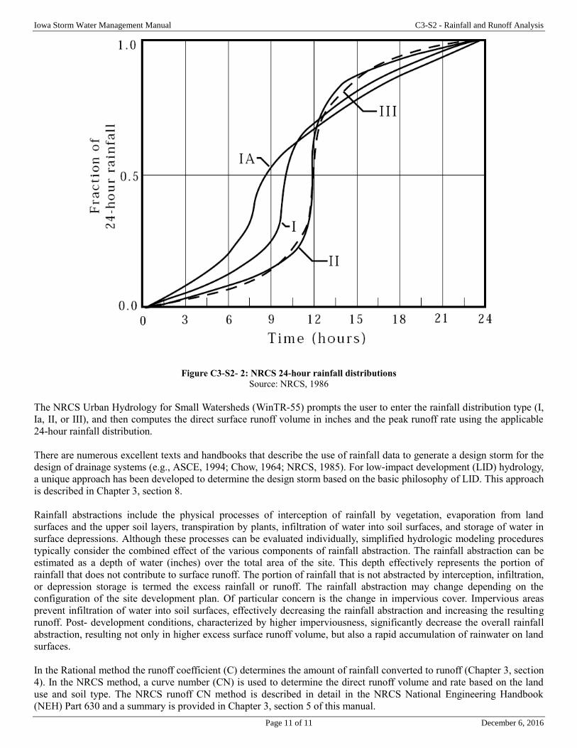
C. NRCS 24-hour storm distribution
The NRCS 24-hour storm distribution curve was derived from the National Weather Bureau's Rainfall Frequency Atlases
of compiled data for areas less than 400 square miles, for durations up to 24 hours, and for frequencies from 1-100 years.
Data analysis resulted in four regional distributions:
Type I and Ia for use in Hawaii, Alaska, and the coastal side of the Sierra Nevada and Cascade Mountains in
California, Washington, and Oregon
Type II distribution for most of the remainder of the United States (including Iowa)
Type III for the Gulf of Mexico and Atlantic coastal areas. The Type III distribution represents the potential
impact of tropical storms which can produce large 24-hour rainfall amounts.
Iowa and all of the upper Midwest fall under the Type II rainfall distribution. For a more detailed description of the
development of dimensionless rainfall distributions, refer to the USDA Soil Conservation Service’s National Engineering
Handbook (NRCS NEH), Part 630, Section 4 - http://directives.sc.egov.usda.gov/viewerFS.aspx?hid=21429.
The NRCS 24-hour storm distributions are based on the generalized rainfall depth-duration-frequency relationships
collected for rainfall events lasting from 30 minutes up to 24 hours. Working in 30- minute increments, the rainfall depths
are arranged with the maximum rainfall depth assumed to occur in the middle of the 24-hour period. The next largest 30-
minute incremental depth occurs just after the maximum depth; the third largest rainfall depth occurs just prior to the
maximum depth, etc. This continues with each decreasing 30-minute incremental depth until the smaller increments fall at
the beginning and end of the 24-hour rainfall (see Figure C3-S2- 2).
The length of the most intense rainfall period contributing to the peak runoff rate is related to the time of concentration
(Tc) for the watershed. In a hydrograph created with NRCS procedures, the duration of rainfall that directly contributes to
the peak is about 170 percent of the Tc. For example, the most intense 8.5-minute rainfall period would contribute to the
peak discharge for a watershed with a Tc of 5 minutes; the most intense 8.5-hour period would contribute to the peak for a
watershed with a 5-hour Tc. To avoid the use of different sets of rainfall intensities for each drainage area size, a set of
synthetic rainfall distributions having “nested” rainfall intensities was developed. The set maximizes the rainfall
intensities by incorporating selected short duration intensities within those needed for longer durations at the same
probability level. For the size of the drainage areas for which NRCS usually provides assistance, a storm period of 24
hours was chosen for the synthetic rainfall distributions. The 24-hour storm, while longer than that needed to determine
peaks for these drainage areas, is appropriate for determining runoff volumes. Therefore, a single storm duration and
associated synthetic rainfall distribution can be used to represent not only the peak discharges, but also the runoff volumes
for a range of drainage area sizes.
Iowa Storm Water Management Manual C3-S2 - Rainfall and Runoff Analysis
Page 11 of 11 December 6, 2016
Figure C3-S2- 2: NRCS 24-hour rainfall distributions
Source: NRCS, 1986
The NRCS Urban Hydrology for Small Watersheds (WinTR-55) prompts the user to enter the rainfall distribution type (I,
Ia, II, or III), and then computes the direct surface runoff volume in inches and the peak runoff rate using the applicable
24-hour rainfall distribution.
There are numerous excellent texts and handbooks that describe the use of rainfall data to generate a design storm for the
design of drainage systems (e.g., ASCE, 1994; Chow, 1964; NRCS, 1985). For low-impact development (LID) hydrology,
a unique approach has been developed to determine the design storm based on the basic philosophy of LID. This approach
is described in Chapter 3, section 8.
Rainfall abstractions include the physical processes of interception of rainfall by vegetation, evaporation from land
surfaces and the upper soil layers, transpiration by plants, infiltration of water into soil surfaces, and storage of water in
surface depressions. Although these processes can be evaluated individually, simplified hydrologic modeling procedures
typically consider the combined effect of the various components of rainfall abstraction. The rainfall abstraction can be
estimated as a depth of water (inches) over the total area of the site. This depth effectively represents the portion of
rainfall that does not contribute to surface runoff. The portion of rainfall that is not abstracted by interception, infiltration,
or depression storage is termed the excess rainfall or runoff. The rainfall abstraction may change depending on the
configuration of the site development plan. Of particular concern is the change in impervious cover. Impervious areas
prevent infiltration of water into soil surfaces, effectively decreasing the rainfall abstraction and increasing the resulting
runoff. Post- development conditions, characterized by higher imperviousness, significantly decrease the overall rainfall
abstraction, resulting not only in higher excess surface runoff volume, but also a rapid accumulation of rainwater on land
surfaces.
In the Rational method the runoff coefficient (C) determines the amount of rainfall converted to runoff (Chapter 3, section
4). In the NRCS method, a curve number (CN) is used to determine the direct runoff volume and rate based on the land
use and soil type. The NRCS runoff CN method is described in detail in the NRCS National Engineering Handbook
(NEH) Part 630 and a summary is provided in Chapter 3, section 5 of this manual.
Page 1 of 14 October 28, 2009
Chapter 3- Section 3 Time of Concentration
A. Introduction
The time of concentration (Tc) is used in numerous equations to calculate discharge, particularly with the Rational
method, WinTR-55, and WinTR-20. In most watersheds, it is necessary to add the many different time of concentrations
resulting from different field conditions that runoff flows through to reach the point of investigation. Water moves through
a watershed as sheet flow, shallow concentrated flow, swales, open channels, street gutters, storm sewers, or some
combination of these. This section describes the many conditions and corresponding solutions that need to be considered
when estimating the total time of concentration (Tc) (sum of runoff travel time).
There are also many methods utilized to estimate the time of concentration. Examples are the Kinematic Wave Method,
Kirpich formula, Kerby formula, and the NRCS Velocity Method. The NRCS Velocity Method is one of the most
common, is easily understood, has continuity with many computer programs, and is considered as accurate as other
methods. It is for these reasons the NRCS Velocity Method is used in this manual. If there is a desire to use a different
method in determining the time of concentration, the Engineer needs to be contacted for approval.
B. Definition
The time of concentration is defined as the time required for water falling on the most remote point of a drainage basin to
reach the outlet where remoteness relates to time of travel rather than distance. Probably a better definition is that it is the
time after the beginning of rainfall excess when all portions of the drainage basin are contributing simultaneously to flow
at the outlet.
Using an appropriate value for time of concentration is very important, although it is hard sometimes to judge what the
correct value is.
The time of concentration is often assumed to be the sum of two travel times (Tt). The first is the initial time required for
the overland flow, and the second is the travel time in the conveyance elements (open channels, street gutters, storm
sewers, etc).
C. Factors affecting time of concentration
1. Surface roughness. One of the most significant effects of urban development on flow velocity is a decrease in
retardance to flow. That is, undeveloped areas with very slow and shallow overland flow through vegetation
become modified by urban development; the flow is then delivered to streets, gutters, and storm sewers that
transport runoff downstream more rapidly. Travel time through the watershed is generally decreased.
2. Channel shape and flow patterns. In small non-urban watersheds, much of the travel time results from overland
flow in upstream areas. Typically, urbanization reduces overland flow lengths by conveying storm runoff into a
channel as soon as possible. Since channel designs have efficient hydraulic characteristics, runoff flow velocity
increases and travel time decreases.
3. Slope. Slopes may be increased or decreased by urbanization, depending on the extent of site grading or the
extent to which storm sewers and street ditches are used in the design of the water management system. Slope will
tend to increase when channels are straightened and decrease when overland flow is directed through storm
sewers, street gutters, and diversions.
D. Estimating time of concentration (NRCS velocity method)
1. Travel time. Travel time (Tt) is the time it takes water to travel from one location to another in a watershed. Tt is a
component of time of concentration (Tc), which is time for runoff to travel from the hydraulically most distant
point of the watershed to a point of interest within the watershed. Tc is computed by summing all the travel times
for consecutive components of the drainage conveyance system.
Tc influences the shape and peak of the runoff hydrograph. Urbanization usually decreases Tc, thereby increasing
Iowa Storm Water Management Manual C3-S3 - Time of Concentration
Page 2 of 14 October 28, 2009
the peak discharge. But Tc can be increased as a result of:
Ponding behind small or inadequate drainage systems, including storm drain inlets and road culverts
Reduction of land slope through grading
Lengthening the flow path
Decreasing the impervious area and/or reducing the directly connected impervious area in the catchment
Travel time (Tt) is the ratio of flow length to flow velocity:
Equation C3-S3- 1
𝑇𝑡 =𝐿
3600𝑉
Where:
Tt = travel time (hours)
L = flow length (ft)
V = average velocity (ft/s)
3600 = conversion factor from seconds to hours
Time of concentration (Tc) is the sum of Tt values for the various consecutive flow segments:
Equation C3-S3- 2
𝑻𝒄 = 𝑻𝒕𝟏 + 𝑻𝒕𝟐 + 𝑻𝒕𝟑 … … 𝑻𝒕𝒎
Where:
Tc = time of concentration (hr)
Tt = travel time for a flow component m = number of flow segments
2. Sheet flow. Sheet flow is flow over plane surfaces (parking lots, farm fields, lawns). It usually occurs in the
headwater of streams. With sheet flow, the friction value (Manning's n) is an effective roughness coefficient that
includes the effect of rain drop impact; drag over the plane surface; obstacles such as litter, vegetation, crop
ridges, and rocks; and erosion and transportation of sediment. These n values are for very shallow flow depths of
about 0.1 foot. Table C3-S3- 1 gives Manning's n values for sheet flow for various surface conditions.
For sheet flow of less than 100 feet, use Manning's kinematic solution (Overton and Meadows, 1976) to compute
Tt;
Equation C3-S3- 3
𝑇𝑡 =0.007[(𝑛)(𝐿)]0.8
√𝑃2𝑆0.4
Where:
Tt = travel time (hours)
n = Manning's roughness coefficient (Table C3-S3- 2)
L = flow length (ft)
P2 = the 2-year, 24-hour rainfall (inches)
S = slope of hydraulic grade line (land slope, ft/ft)
This simplified form of Manning's kinematic solution is based on the following:
Shallow steady uniform flow
Constant intensity of rainfall excess (that part of a rain available for runoff)
Rainfall duration of 24 hours
Iowa Storm Water Management Manual C3-S3 - Time of Concentration
Page 3 of 14 October 28, 2009
Minor effect of infiltration on travel time
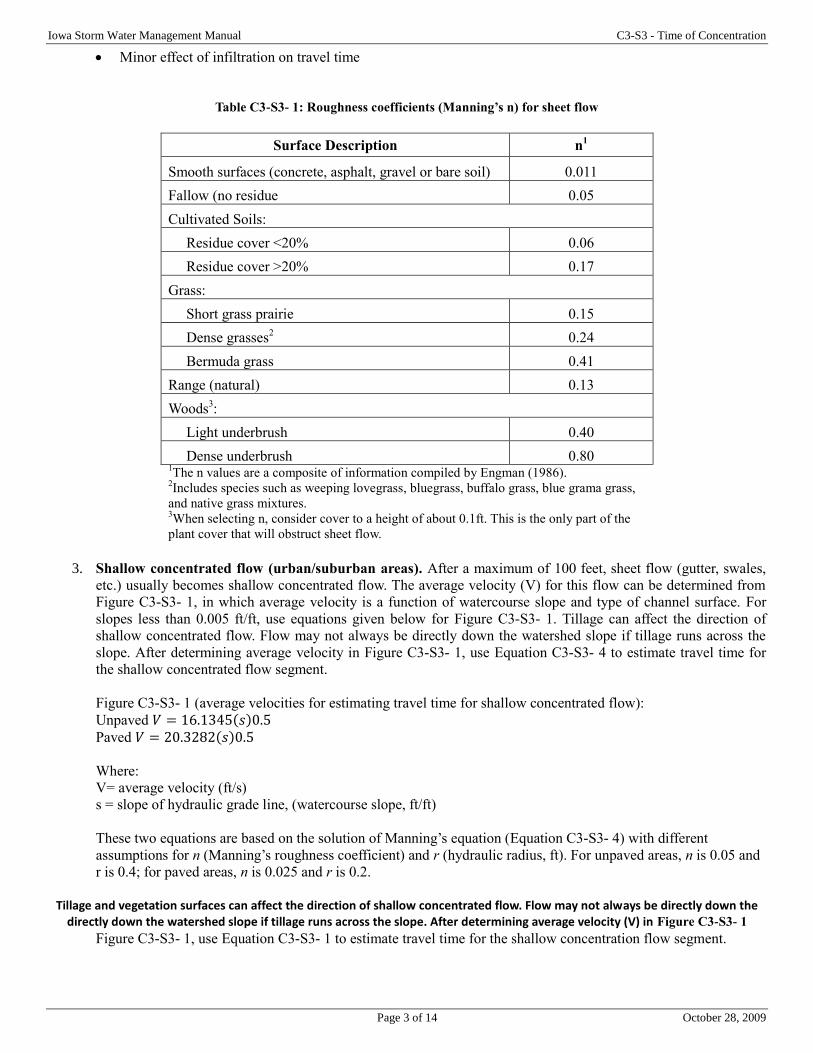
Table C3-S3- 1: Roughness coefficients (Manning’s n) for sheet flow
Surface Description n1
Smooth surfaces (concrete, asphalt, gravel or bare soil) 0.011
Fallow (no residue 0.05
Cultivated Soils:
Residue cover <20% 0.06
Residue cover >20% 0.17
Grass:
Short grass prairie 0.15
Dense grasses2 0.24
Bermuda grass 0.41
Range (natural) 0.13
Woods3:
Light underbrush 0.40
Dense underbrush 0.80 1The n values are a composite of information compiled by Engman (1986).
2Includes species such as weeping lovegrass, bluegrass, buffalo grass, blue grama grass,
and native grass mixtures. 3When selecting n, consider cover to a height of about 0.1ft. This is the only part of the
plant cover that will obstruct sheet flow.
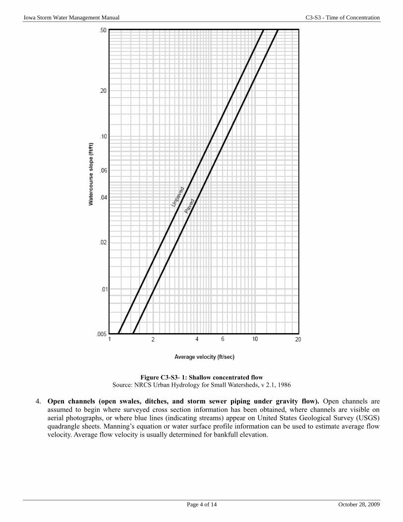
3. Shallow concentrated flow (urban/suburban areas). After a maximum of 100 feet, sheet flow (gutter, swales,
etc.) usually becomes shallow concentrated flow. The average velocity (V) for this flow can be determined from
Figure C3-S3- 1, in which average velocity is a function of watercourse slope and type of channel surface. For
slopes less than 0.005 ft/ft, use equations given below for Figure C3-S3- 1. Tillage can affect the direction of
shallow concentrated flow. Flow may not always be directly down the watershed slope if tillage runs across the
slope. After determining average velocity in Figure C3-S3- 1, use Equation C3-S3- 4 to estimate travel time for
the shallow concentrated flow segment.
Figure C3-S3- 1 (average velocities for estimating travel time for shallow concentrated flow):
Unpaved 𝑉 = 16.1345(𝑠)0.5
Paved 𝑉 = 20.3282(𝑠)0.5
Where:
V= average velocity (ft/s)
s = slope of hydraulic grade line, (watercourse slope, ft/ft)
These two equations are based on the solution of Manning’s equation (Equation C3-S3- 4) with different
assumptions for n (Manning’s roughness coefficient) and r (hydraulic radius, ft). For unpaved areas, n is 0.05 and
r is 0.4; for paved areas, n is 0.025 and r is 0.2.
Tillage and vegetation surfaces can affect the direction of shallow concentrated flow. Flow may not always be directly down the directly down the watershed slope if tillage runs across the slope. After determining average velocity (V) in Figure C3-S3- 1
Figure C3-S3- 1, use Equation C3-S3- 1 to estimate travel time for the shallow concentration flow segment.
Iowa Storm Water Management Manual C3-S3 - Time of Concentration
Page 4 of 14 October 28, 2009
Figure C3-S3- 1: Shallow concentrated flow
Source: NRCS Urban Hydrology for Small Watersheds, v 2.1, 1986
4. Open channels (open swales, ditches, and storm sewer piping under gravity flow). Open channels are
assumed to begin where surveyed cross section information has been obtained, where channels are visible on
aerial photographs, or where blue lines (indicating streams) appear on United States Geological Survey (USGS)
quadrangle sheets. Manning’s equation or water surface profile information can be used to estimate average flow
velocity. Average flow velocity is usually determined for bankfull elevation.
Iowa Storm Water Management Manual C3-S3 - Time of Concentration
Page 5 of 14 October 28, 2009
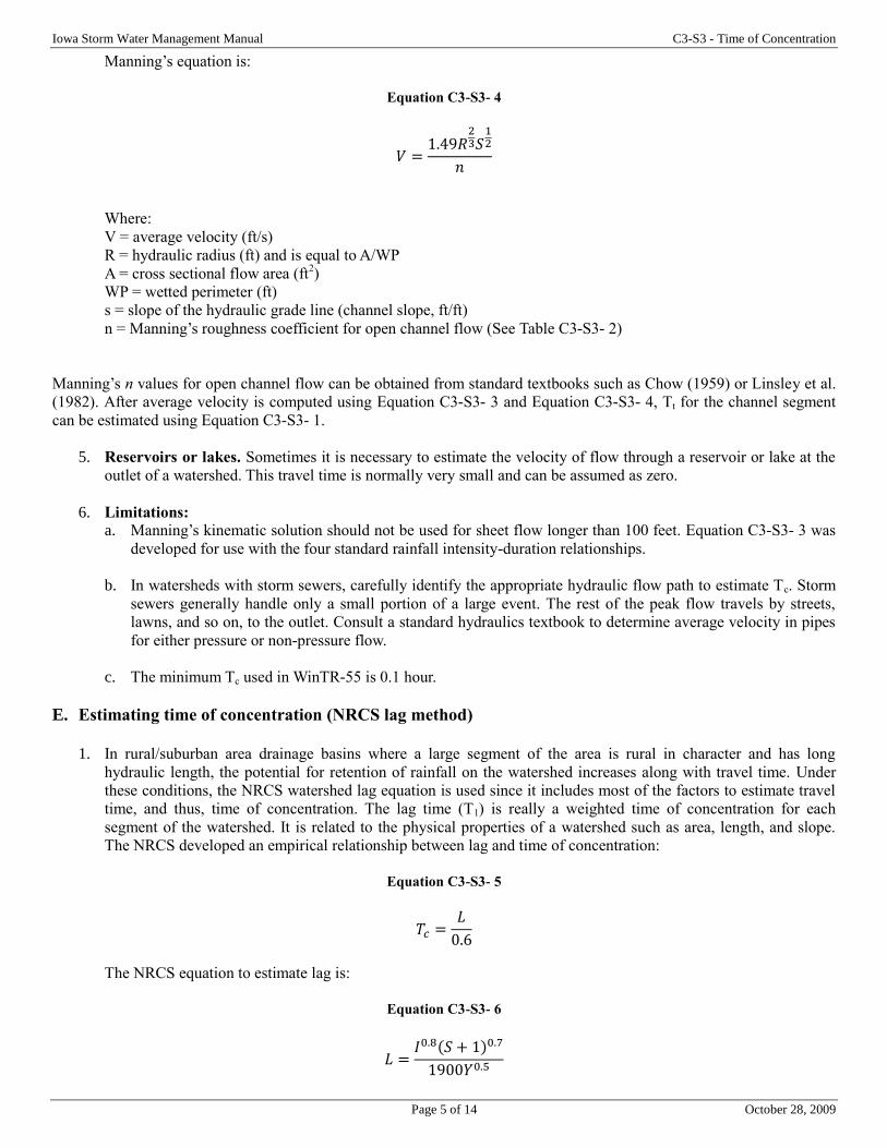
Manning’s equation is:
Equation C3-S3- 4
𝑉 =1.49𝑅
23𝑆
12
𝑛
Where:
V = average velocity (ft/s)
R = hydraulic radius (ft) and is equal to A/WP
A = cross sectional flow area (ft2)
WP = wetted perimeter (ft)
s = slope of the hydraulic grade line (channel slope, ft/ft)
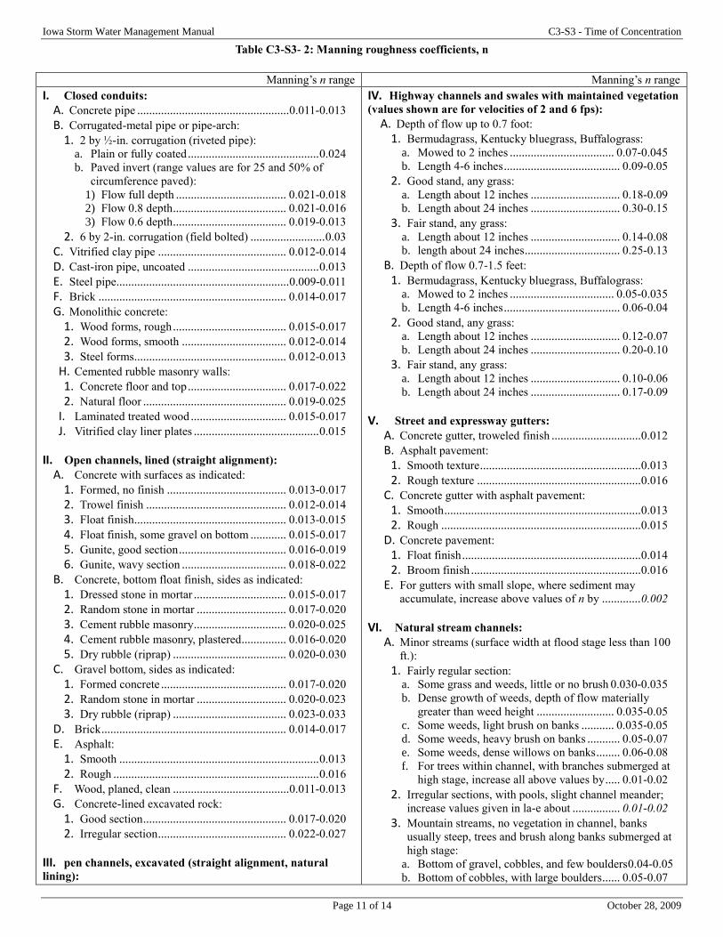
n = Manning’s roughness coefficient for open channel flow (See Table C3-S3- 2)
Manning’s n values for open channel flow can be obtained from standard textbooks such as Chow (1959) or Linsley et al.
(1982). After average velocity is computed using Equation C3-S3- 3 and Equation C3-S3- 4, Tt for the channel segment
can be estimated using Equation C3-S3- 1.
5. Reservoirs or lakes. Sometimes it is necessary to estimate the velocity of flow through a reservoir or lake at the
outlet of a watershed. This travel time is normally very small and can be assumed as zero.
6. Limitations:
a. Manning’s kinematic solution should not be used for sheet flow longer than 100 feet. Equation C3-S3- 3 was
developed for use with the four standard rainfall intensity-duration relationships.
b. In watersheds with storm sewers, carefully identify the appropriate hydraulic flow path to estimate Tc. Storm
sewers generally handle only a small portion of a large event. The rest of the peak flow travels by streets,
lawns, and so on, to the outlet. Consult a standard hydraulics textbook to determine average velocity in pipes
for either pressure or non-pressure flow.
c. The minimum Tc used in WinTR-55 is 0.1 hour.
E. Estimating time of concentration (NRCS lag method)
1. In rural/suburban area drainage basins where a large segment of the area is rural in character and has long
hydraulic length, the potential for retention of rainfall on the watershed increases along with travel time. Under
these conditions, the NRCS watershed lag equation is used since it includes most of the factors to estimate travel
time, and thus, time of concentration. The lag time (T1) is really a weighted time of concentration for each
segment of the watershed. It is related to the physical properties of a watershed such as area, length, and slope.
The NRCS developed an empirical relationship between lag and time of concentration:
Equation C3-S3- 5
𝑇𝑐 =𝐿
0.6
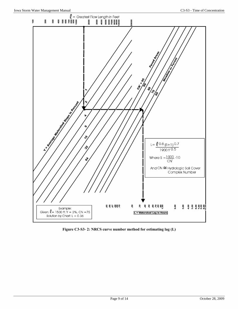
The NRCS equation to estimate lag is:
Equation C3-S3- 6
𝐿 =𝐼0.8(𝑆 + 1)0.7
1900𝑌0.5
Iowa Storm Water Management Manual C3-S3 - Time of Concentration
Page 6 of 14 October 28, 2009
Where:
Tc = time of concentration (hr)
l = hydraulic length of watershed (ft)
L = basin lag (hr)
S = (1000/CN)-10 where CN = NRCS curve number (See Table C3-S3- 2)
Y = average watershed land slope (percent)
2. Hydraulic length of watershed. Watershed lag is a function of the hydraulic length of the watershed, the
potential maximum retention of rainfall on the watershed and the average land slope of the watershed. The
potential retention, S, is a function of the runoff curve number.
The hydraulic length of the watershed, L, is the length from the point of design along the main channel to the
ridgeline at the upper end of the watershed. At one or more points along its length moving upstream, the main
channel may appear to divide into two channels. The main channel is then defined as that channel which drains
the greater tributary drainage area. This same definition is used for all further upstream channel divisions until the
watershed ridgeline is reached.
Since many channels meander through their floodplains, and since most designs are based on floods which exceed
channel capacity, the proper channel length to use is actually the length along the valley; i.e., the channel
meanders should be ignored.
The average watershed land slope, Y, is just that and is estimated using one of the two methods described on the
following two pages. These pages were excerpted from a user’s guide to TR-55 prepared by the state office of
NRCS in Iowa.
a. Computing average watershed slope. Average watershed slope is a variable, which is usually not readily
apparent. Therefore, a systematic procedure for finding slope is desirable. Several observations or map
measurements are commonly needed. Reasonable care should be taken in determining this parameter as peak
discharge and hydrograph shape are sensitive to the value used for watershed slope. Best hydrologic results
are obtained when the slope value represents a weighted average for the area. Two methods for computing
slope are demonstrated in example exercises below. Remember, watershed slope is not the same as stream
gradient.
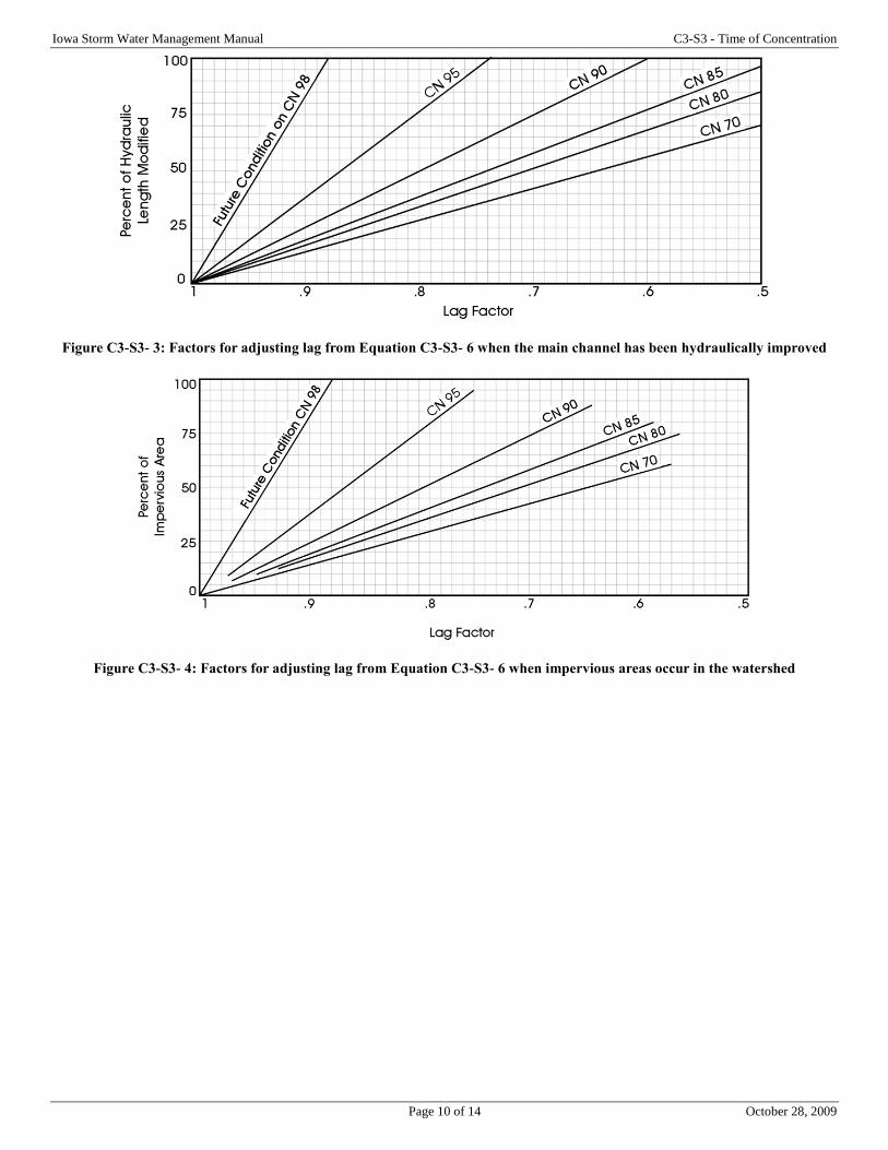
b. Watershed lag. The lag equation was developed for rural areas and thus overestimates lag and Tc in urban areas for two reasons. First, the increased amount of impervious area permits water from overland flow sources and side channels to reach the main channel at a much faster rate than under natural conditions. Second is the extent to which a stream (usually the major watercourse in the watershed) has been changed over natural conditions to allow higher flow velocities. The lag time can be corrected for the effects of urbanization by using Figure C3-S3- 3 and Figure C3-S3- 4. The amount of modification to the hydraulic flow length must usually be determined from topographic maps or aerial photographs following a filed inspection of the drainage area.
c. Estimating lag and time of concentration. Figure C3-S3- 2 may be used to estimate lag, and Equation C3-
S3- 3 to estimate time of concentration. The NRCS EFH-2 Computer program is a Windows program which
computed runoff and peak discharge. Peak discharges are determined using the lag equation. The program
will compute the time of concentration, and the nomograph in Figure C3-S3- 2 is not used. The NRCS EFH-2
program can be downloaded at:
http://www.nrcs.usda.gov/wps/portal/nrcs/detailfull/national/water/?cid=stelprdb1042921. The limitations of
the lag method for determining time of concentration, runoff volume, and peak rate are listed below.
d. Limitations for using the NRCS lag method for Tc and runoff determination:
1) The watershed drainage area must be greater than 1 acre, and less than 2,000 acres. If the drainage area
is outside these limits, another procedure such as WinTR-55 or WinTR-20, Project Formulation-
Hydrology, should be used to estimate peak discharge.
Iowa Storm Water Management Manual C3-S3 - Time of Concentration
Page 7 of 14 October 28, 2009
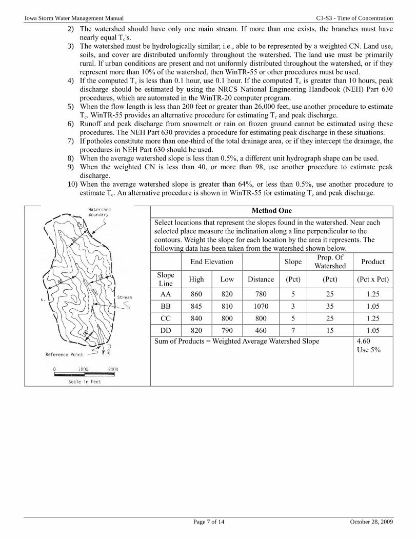
2) The watershed should have only one main stream. If more than one exists, the branches must have
nearly equal Tc's.
3) The watershed must be hydrologically similar; i.e., able to be represented by a weighted CN. Land use,
soils, and cover are distributed uniformly throughout the watershed. The land use must be primarily
rural. If urban conditions are present and not uniformly distributed throughout the watershed, or if they
represent more than 10% of the watershed, then WinTR-55 or other procedures must be used.
4) If the computed Tc is less than 0.1 hour, use 0.1 hour. If the computed Tc is greater than 10 hours, peak
discharge should be estimated by using the NRCS National Engineering Handbook (NEH) Part 630
procedures, which are automated in the WinTR-20 computer program.
5) When the flow length is less than 200 feet or greater than 26,000 feet, use another procedure to estimate
Tc. WinTR-55 provides an alternative procedure for estimating Tc and peak discharge.
6) Runoff and peak discharge from snowmelt or rain on frozen ground cannot be estimated using these
procedures. The NEH Part 630 provides a procedure for estimating peak discharge in these situations.
7) If potholes constitute more than one-third of the total drainage area, or if they intercept the drainage, the
procedures in NEH Part 630 should be used.
8) When the average watershed slope is less than 0.5%, a different unit hydrograph shape can be used.
9) When the weighted CN is less than 40, or more than 98, use another procedure to estimate peak
discharge.
10) When the average watershed slope is greater than 64%, or less than 0.5%, use another procedure to
estimate Tc. An alternative procedure is shown in WinTR-55 for estimating Tc and peak discharge.
Method One
Select locations that represent the slopes found in the watershed. Near each
selected place measure the inclination along a line perpendicular to the
contours. Weight the slope for each location by the area it represents. The
following data has been taken from the watershed shown below.
End Elevation Slope Prop. Of
Watershed Product
Slope
Line High Low Distance (Pct) (Pct) (Pct x Pct)
AA 860 820 780 5 25 1.25
BB 845 810 1070 3 35 1.05
CC 840 800 800 5 25 1.25
DD 820 790 460 7 15 1.05
Sum of Products = Weighted Average Watershed Slope 4.60
Use 5%

Iowa Storm Water Management Manual C3-S3 - Time of Concentration
Page 8 of 14 October 28, 2009
Method Two
In this method, each sample location represents the same proportion of the
watershed. Select the locations by overlaying the map with a grid system. The
watershed slop perpendicular to contours through each intersection of grid
lines is determined as in Method One and the average for all intersections is
considered to be watershed slope. The watershed used as an example for this
method is the same watershed as above. A grid system with numbered
intersections is shown in the figure. Tabulations below demonstrate use of
this procedure.
Location 1 2 3 4 5 6 7 8 Su
m
Slope (%) 6 8 6 7 5 10 3 6 51
The Weighted Average Watershed Slop is the arithmetic average, 6.4%. Use
6%.
The two answers are not identical. Due to the greater number of sample
locations used in Method Two, perhaps the answer of 6% watershed slope is
more accurate.
When sub-areas of a watershed have widely varying slopes, this may justify
separate analyses by sub-areas and use of the hydrograph method for
hydrologic data at the watershed outlet. With other parameters held constant,
a slope variation of 10% affects peak discharge approximately 3-4%. A 20%
change in slope is reflected by a 6-8% change in the peak rate.
Iowa Storm Water Management Manual C3-S3 - Time of Concentration
Page 9 of 14 October 28, 2009
Figure C3-S3- 2: NRCS curve number method for estimating lag (L)
Iowa Storm Water Management Manual C3-S3 - Time of Concentration
Page 10 of 14 October 28, 2009
Figure C3-S3- 3: Factors for adjusting lag from Equation C3-S3- 6 when the main channel has been hydraulically improved
Figure C3-S3- 4: Factors for adjusting lag from Equation C3-S3- 6 when impervious areas occur in the watershed
Iowa Storm Water Management Manual C3-S3 - Time of Concentration
Page 11 of 14 October 28, 2009
Table C3-S3- 2: Manning roughness coefficients, n
Manning’s n range Manning’s n range
I. Closed conduits:
A. Concrete pipe ................................................... 0.011-0.013
B. Corrugated-metal pipe or pipe-arch:
1. 2 by ½-in. corrugation (riveted pipe):
a. Plain or fully coated ............................................ 0.024
b. Paved invert (range values are for 25 and 50% of
circumference paved):
1) Flow full depth ..................................... 0.021-0.018
2) Flow 0.8 depth ...................................... 0.021-0.016
3) Flow 0.6 depth ...................................... 0.019-0.013
2. 6 by 2-in. corrugation (field bolted) ......................... 0.03
C. Vitrified clay pipe ........................................... 0.012-0.014
D. Cast-iron pipe, uncoated ............................................ 0.013
E. Steel pipe.......................................................... 0.009-0.011
F. Brick ............................................................... 0.014-0.017
G. Monolithic concrete:
1. Wood forms, rough ...................................... 0.015-0.017
2. Wood forms, smooth ................................... 0.012-0.014
3. Steel forms................................................... 0.012-0.013
H. Cemented rubble masonry walls:
1. Concrete floor and top ................................. 0.017-0.022
2. Natural floor ................................................ 0.019-0.025
I. Laminated treated wood ................................ 0.015-0.017
J. Vitrified clay liner plates .......................................... 0.015
II. Open channels, lined (straight alignment):
A. Concrete with surfaces as indicated:
1. Formed, no finish ........................................ 0.013-0.017
2. Trowel finish ............................................... 0.012-0.014
3. Float finish................................................... 0.013-0.015
4. Float finish, some gravel on bottom ............ 0.015-0.017
5. Gunite, good section .................................... 0.016-0.019
6. Gunite, wavy section ................................... 0.018-0.022
B. Concrete, bottom float finish, sides as indicated:
1. Dressed stone in mortar ............................... 0.015-0.017
2. Random stone in mortar .............................. 0.017-0.020
3. Cement rubble masonry ............................... 0.020-0.025
4. Cement rubble masonry, plastered ............... 0.016-0.020
5. Dry rubble (riprap) ...................................... 0.020-0.030
C. Gravel bottom, sides as indicated:
1. Formed concrete .......................................... 0.017-0.020
2. Random stone in mortar .............................. 0.020-0.023
3. Dry rubble (riprap) ...................................... 0.023-0.033
D. Brick .............................................................. 0.014-0.017
E. Asphalt:
1. Smooth ................................................................... 0.013
2. Rough ..................................................................... 0.016
F. Wood, planed, clean ....................................... 0.011-0.013
G. Concrete-lined excavated rock:
1. Good section ................................................ 0.017-0.020
2. Irregular section ........................................... 0.022-0.027
III. pen channels, excavated (straight alignment, natural
lining):
IV. Highway channels and swales with maintained vegetation
(values shown are for velocities of 2 and 6 fps):
A. Depth of flow up to 0.7 foot:
1. Bermudagrass, Kentucky bluegrass, Buffalograss:
a. Mowed to 2 inches ................................... 0.07-0.045
b. Length 4-6 inches ....................................... 0.09-0.05
2. Good stand, any grass:
a. Length about 12 inches .............................. 0.18-0.09
b. Length about 24 inches .............................. 0.30-0.15
3. Fair stand, any grass:
a. Length about 12 inches .............................. 0.14-0.08
b. length about 24 inches ................................ 0.25-0.13
B. Depth of flow 0.7-1.5 feet:
1. Bermudagrass, Kentucky bluegrass, Buffalograss:
a. Mowed to 2 inches ................................... 0.05-0.035
b. Length 4-6 inches ....................................... 0.06-0.04
2. Good stand, any grass:
a. Length about 12 inches .............................. 0.12-0.07
b. Length about 24 inches .............................. 0.20-0.10
3. Fair stand, any grass:
a. Length about 12 inches .............................. 0.10-0.06
b. Length about 24 inches .............................. 0.17-0.09
V. Street and expressway gutters:
A. Concrete gutter, troweled finish .............................. 0.012
B. Asphalt pavement:
1. Smooth texture ...................................................... 0.013
2. Rough texture ....................................................... 0.016
C. Concrete gutter with asphalt pavement:
1. Smooth .................................................................. 0.013
2. Rough ................................................................... 0.015
D. Concrete pavement:
1. Float finish ............................................................ 0.014
2. Broom finish ......................................................... 0.016
E. For gutters with small slope, where sediment may
accumulate, increase above values of n by ............. 0.002
VI. Natural stream channels:
A. Minor streams (surface width at flood stage less than 100
ft.):
1. Fairly regular section:
a. Some grass and weeds, little or no brush 0.030-0.035
b. Dense growth of weeds, depth of flow materially
greater than weed height .......................... 0.035-0.05
c. Some weeds, light brush on banks ........... 0.035-0.05
d. Some weeds, heavy brush on banks ........... 0.05-0.07
e. Some weeds, dense willows on banks ........ 0.06-0.08
f. For trees within channel, with branches submerged at
high stage, increase all above values by ..... 0.01-0.02
2. Irregular sections, with pools, slight channel meander;
increase values given in la-e about ................ 0.01-0.02
3. Mountain streams, no vegetation in channel, banks
usually steep, trees and brush along banks submerged at
high stage:
a. Bottom of gravel, cobbles, and few boulders0.04-0.05
b. Bottom of cobbles, with large boulders ...... 0.05-0.07
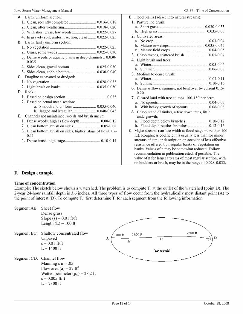
Iowa Storm Water Management Manual C3-S3 - Time of Concentration
Page 12 of 14 October 28, 2009
A. Earth, uniform section:
1. Clean, recently completed ........................... 0.016-0.018
2. Clean, after weathering ................................ 0.018-0.020
3. With short grass, few weeds ........................ 0.022-0.027
4. In gravely soil, uniform section, clean ........ 0.022-0.025
B. Earth, fairly uniform section:
1. No vegetation .............................................. 0.022-0.025
2. Grass, some weeds ...................................... 0.025-0.030
3. Dense weeds or aquatic plants in deep channels .. 0.030-
0.035
4. Sides clean, gravel bottom ........................... 0.025-0.030
5. Sides clean, cobble bottom .......................... 0.030-0.040
C. Dragline excavated or dredged:
1. No vegetation .............................................. 0.028-0.033
2. Light brush on banks ................................... 0.035-0.050
D. Rock:
1. Based on design section ......................................... 0.035
2. Based on actual mean section:
a. Smooth and uniform ....................... 0.035-0.040
b. Jagged and irregular ........................ 0.040-0.045
E. Channels not maintained, weeds and brush uncut:
1. Dense weeds, high as flow depth .................... 0.08-0.12
2. Clean bottom, brush on sides........................... 0.05-0.08
3. Clean bottom, brush on sides, highest stage of flow0.07-
0.11
4. Dense brush, high stage ................................... 0.10-0.14
B. Flood plains (adjacent to natural streams):
1. Pasture, no brush:
a. Short grass .............................................. 0.030-0.035
b. High grass ................................................ 0.035-0.05
2. Cultivated areas:
a. No crop....................................................... 0.03-0.04
b. Mature row crops ................................... 0.035-0.045
c. Mature field crops ...................................... 0.04-0.05
3. Heavy weeds, scattered brush ........................ 0.05-0.07
4. Light brush and trees:
a. Winter ......................................................... 0.05-0.06
b. Summer ...................................................... 0.06-0.08
5. Medium to dense brush:
a. Winter ......................................................... 0.07-0.11
b. Summer ...................................................... 0.10-0.16
6. Dense willows, summer, not bent over by current 0.15-
0.20
7. Cleared land with tree stumps, 100-150 per acre:
a. No sprouts .................................................. 0.04-0.05
b. With heavy growth of sprouts .................... 0.06-0.08
8. Heavy stand of timber, a few down trees, little
undergrowth:
a. Flood depth below branches ....................... 0.10-0.12
b. Flood depth reaches branches .................... 0.12-0.16
C. Major streams (surface width at flood stage more than 100
ft.): Roughness coefficient is usually less than for minor
streams of similar description on account of less effective
resistance offered by irregular banks of vegetation on
banks. Values of n may be somewhat reduced. Follow
recommendation in publication cited, if possible. The
value of n for larger streams of most regular section, with
no boulders or brush, may be in the range of 0.028-0.033.
F. Design example
Time of concentration
Example: The sketch below shows a watershed. The problem is to compute Tc at the outlet of the watershed (point D). The
2-year 24-hour rainfall depth is 3.6 inches. All three types of flow occur from the hydraulically most distant point (A) to
the point of interest (D). To compute Tc, first determine Tt for each segment from the following information:
Segment AB: Sheet flow
Dense grass
Slope (s) = 0.01 ft/ft
Length (L) = 100 ft
Segment BC: Shallow concentrated flow
Unpaved
s = 0.01 ft/ft
L = 1400 ft
Segment CD: Channel flow
Manning’s n = .05
Flow area (a) = 27 ft2
Wetted perimeter (pw) = 28.2 ft
s = 0.005 ft/ft
L = 7300 ft
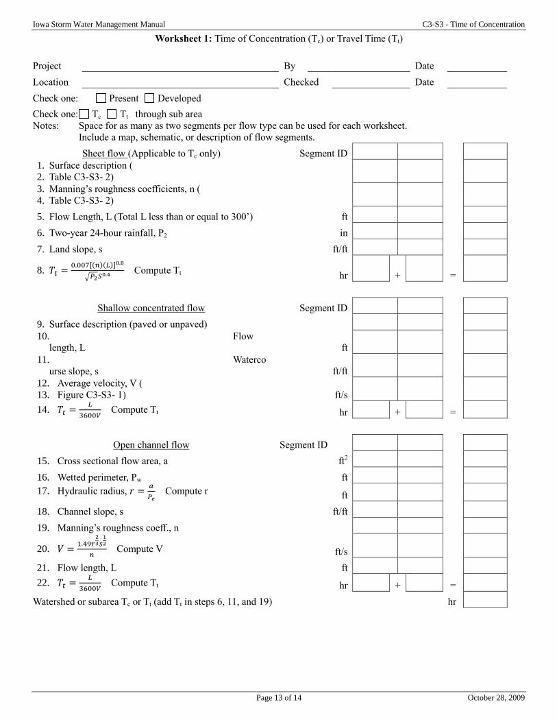
Iowa Storm Water Management Manual C3-S3 - Time of Concentration
Page 13 of 14 October 28, 2009
Worksheet 1: Time of Concentration (Tc) or Travel Time (Tt)
Project By Date
Location Checked Date
Check one: Present Developed
Check one: Tc Tt through sub area
Notes: Space for as many as two segments per flow type can be used for each worksheet.
Include a map, schematic, or description of flow segments.
Sheet flow (Applicable to Tc only) Segment ID
1. Surface description (
2. Table C3-S3- 2)
3. Manning’s roughness coefficients, n (
4. Table C3-S3- 2)
5. Flow Length, L (Total L less than or equal to 300’) ft
6. Two-year 24-hour rainfall, P2 in
7. Land slope, s ft/ft
8. 𝑇𝑡 =0.007[(𝑛)(𝐿)]0.8
√𝑃2𝑆0.4 Compute Tt hr + =
Shallow concentrated flow Segment ID
9. Surface description (paved or unpaved)
10. Flow
length, L ft
11. Waterco
urse slope, s ft/ft
12. Average velocity, V (
13. Figure C3-S3- 1) ft/s
14. 𝑇𝑡 =𝐿
3600𝑉 Compute Tt hr + =
Open channel flow Segment ID
15. Cross sectional flow area, a ft2
16. Wetted perimeter, Pw ft
17. Hydraulic radius, 𝑟 =𝑎
𝑃𝑒 Compute r ft
18. Channel slope, s ft/ft
19. Manning’s roughness coeff., n
20. 𝑉 =1.49𝑟
23𝑠
12
𝑛 Compute V ft/s
21. Flow length, L ft
22. 𝑇𝑡 =𝐿
3600𝑉 Compute Tt hr + =
Watershed or subarea Tc or Tt (add Tt in steps 6, 11, and 19) hr
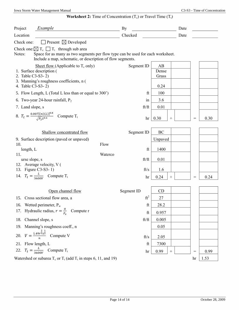
Iowa Storm Water Management Manual C3-S3 - Time of Concentration
Page 14 of 14 October 28, 2009
Worksheet 2: Time of Concentration (Tc) or Travel Time (Tt)
Project Example By Date
Location Checked Date
Check one: Present Developed
Check one: Tc Tt through sub area
Notes: Space for as many as two segments per flow type can be used for each worksheet.
Include a map, schematic, or description of flow segments.
Sheet flow (Applicable to Tc only) Segment ID AB
1. Surface description (
2. Table C3-S3- 2)
Dense
Grass
3. Manning’s roughness coefficients, n (
4. Table C3-S3- 2) 0.24
5. Flow Length, L (Total L less than or equal to 300’) ft 100
6. Two-year 24-hour rainfall, P2 in 3.6
7. Land slope, s ft/ft 0.01
8. 𝑇𝑡 =0.007[(𝑛)(𝐿)]0.8
√𝑃2𝑆0.4 Compute Tt hr 0.30 + = 0.30
Shallow concentrated flow Segment ID BC
9. Surface description (paved or unpaved) Unpaved
10. Flow
length, L ft 1400
11. Waterco
urse slope, s ft/ft 0.01
12. Average velocity, V (
13. Figure C3-S3- 1) ft/s 1.6
14. 𝑇𝑡 =𝐿
3600𝑉 Compute Tt hr 0.24 + = 0.24
Open channel flow Segment ID CD
15. Cross sectional flow area, a ft2 27
16. Wetted perimeter, Pw ft 28.2
17. Hydraulic radius, 𝑟 =𝑎
𝑃𝑒 Compute r ft 0.957
18. Channel slope, s ft/ft 0.005
19. Manning’s roughness coeff., n 0.05
20. 𝑉 =1.49𝑟
23𝑠
12
𝑛 Compute V ft/s 2.05
21. Flow length, L ft 7300
22. 𝑇𝑡 =𝐿
3600𝑉 Compute Tt hr 0.99 + = 0.99
Watershed or subarea Tc or Tt (add Tt in steps 6, 11, and 19) hr 1.53
Page 1 of 7 October 28, 2009
Chapter 3- Section 4 Rational Method
A. Introduction
The Rational method is based upon the following formula:
Equation C3-S4- 1
𝑄𝑇 = 𝐶𝑖𝑇𝐴
Where:
QT = estimate of the peak rate of runoff (cfs) for some recurrence interval, T
C = runoff coefficient; fraction of runoff, expressed as a dimensionless decimal fraction, that appears as surface runoff
from the contributing drainage area.
iT = average rainfall intensity (in/hr) for some recurrence interval, T during that period of time equal to Tc.
A= the contributing tributary drainage area to the point of design in acres which produces the maximum peak rate of
runoff
Tc = rainfall intensity averaging time in minutes
Rainfall intensity averaging time is used as the definition of Tc in this instance because it more accurately describes the
only use for this variable (i.e., to estimate a time during a storm in which the average rainfall intensity is at maximum. The
time is defined as the time required for water to travel from the hydraulically most distant point in the contributing
drainage area to the point of design.
B. Characteristics
1. When using the Rational formula, an assumption is made that maximum rate of flow is produced by a constant
rainfall, which is maintained for a time equal to the period of concentration of flow at the point under
consideration. Theoretically, this is the time of concentration, which is the time required for the surface runoff
from the most remote part of the drainage basin to reach the point being considered. However, in practice, the
concentration time is an empirical value that results in acceptable peak flow estimates. There are other
assumptions used in the Rational method, and thus the designer or engineer should consider how exceptions or
other unusual circumstances might affect those results:
a. The recurrence interval of the peak flow rate is the same as that of the average rainfall intensity.
b. The rainfall is uniform in space over the drainage area being considered.
c. The rainfall intensity remains constant during the time period equal to the rainfall intensity averaging time.
d. The storm duration associated with the peak flow rate is equal to the rainfall intensity during the rainfall
intensity averaging time to that point.
e. The runoff frequency curve is parallel to the rainfall frequency curve. This implies that the same value of the
runoff coefficient is used for all recurrence intervals. In practice, the runoff coefficient is adjusted with a
frequency coefficient (Cf) for the 25-year through 100-year recurrence intervals.
f. The drainage area is the total area tributary to the point of design.
g. The rainfall intensity averaging time is the time required for the runoff to flow from the hydraulically most
distant point in the contributing drainage area to the point of design.
2. The following are additional factors that might not normally be considered, yet could prove important:
a. The storm duration gives the length of time over which the average rainfall intensity (iT) persists. Neither the
storm duration nor iT say anything about how the intensity varies during the storm, nor do they consider how
much rain fell before the period in question.
b. A 20% increase or decrease in the value of C has the same effect as changing a 5-year recurrence interval to a
15-year or a 2-year interval, respectively.
c. The chance of all design assumptions being satisfied simultaneously is less than the chance that the rainfall
rate used in the design will actually occur. This, in effect, creates a built-in factor of safety.
d. Another built-in factor of safety is the usual design practice of having the hydraulic gradeline near the top of
the pipe or box. Since the top of the storm sewer pipe is always a few feet lower than the street elevation, a
rainfall intensity greater than the intensity for which the sewer is designed does not automatically mean that
flooding will occur.

Iowa Storm Water Management Manual C3-S4 - Rational Method
Page 2 of 7 October 28, 2009
e. A difference can exist between intense point rainfall (rainfall over a small area) and mean catchment area
rainfall (average rainfall). For that reason, the Rational method should be applied to drainage areas less than
160 acres.
f. In an irregularly-shaped drainage area, a part of the area that has a short time of concentration (Tc) may cause
a greater runoff rate (Q) at the intake or other design point) than the runoff rate calculated for the entire area.
This is because parts of the area with long concentration times are far less susceptible to high-intensity
rainfall. Thus, they skew the calculation.
g. A portion of a drainage area which has a value of C much higher than the rest of the area may produce a
greater amount of runoff at a design point than that calculated for the entire area. This effect is similar to that
described above. In the design of storm sewers for small subbasin areas such as a cul-de-sac in a subdivision,
the designer should be aware that an extremely short time of concentration will result in a high estimate of the
rainfall intensity and the peak rate of runoff. The time of concentration estimates should be checked to make
sure they are reasonable.
h. In some cases, runoff from a portion of the drainage area that is highly-impervious may result in a greater
peak discharge than would occur if the entire area was considered. In these cases, adjustments can be made to
the drainage area by disregarding those areas where flow time is too slow to add to the peak discharge.
Sometimes it is necessary to estimate several different times of concentration to determine the design flow
that is critical for a particular application.
i. When designing a drainage system, the overland flow path is not necessarily the same before and after
development and grading operations have been completed. Selecting overland flow paths in excess of 100 feet
in urban areas and 300 feet in rural areas should be done only after careful consideration.
C. Limitations
The use of the rational formula is subject to several limitations and procedural issues in its use:
The most important limitation is that the only output from the method is a peak discharge (the method provides
only an estimate of a single point on the runoff hydrograph).
The simplest application of the method permits and requires the wide latitude of subjective judgment by the user
in its application. Therefore, the results are difficult to replicate.
The average rainfall intensities used in the formula have no time sequence relation to the actual rainfall pattern
during the storm.
The computation of Tc should include the overland flow time, plus the time of flow in open and/or closed
channels to the point of design.
The runoff coefficient, C, is usually estimated from a table of values (See Table C3-S4- 1). The user must use
good judgment when evaluating the land use in the drainage area under consideration. Note in Table C3-S4- 1,
that the value of C will vary with the return frequency.
Many users assume the entire drainage area is the value to be entered in the Rational method equation. In some
cases, the runoff from the only the interconnected impervious area yields the larger peak flow rate.
D. Use of the Rational method
1. Runoff coefficient. The runoff coefficient (C) represents the integrated effects of infiltration, evaporation,
retention, flow routing, and interception; all of which affect the time distribution and peak rate of runoff. The
runoff coefficient is the variable of the Rational method least-susceptible to precise determination and requires
judgment and understanding on the part of the designer. While engineering judgment will always be required in
the selection of runoff coefficients, a typical coefficient represents the integrated effects of many drainage basin
parameters. The Engineer should realize that the C values shown in Table C3-S4- 1 are typical values, and may
have to be adjusted if the site deviates from typical conditions such as an increase or decrease in percent
impervious.
The values are presented for different surface characteristics, as well as for different aggregate land uses. The
coefficient for various surface areas can be used to develop a composite value for a different land use. The runoff
values for business, residential, industrial, schools, and railroad yard areas are an average of all surfaces typically
found in the particular land use.
The hydrologic soil groups, as defined by NRCS soil scientists and used in Table C3-S4- 1 are:
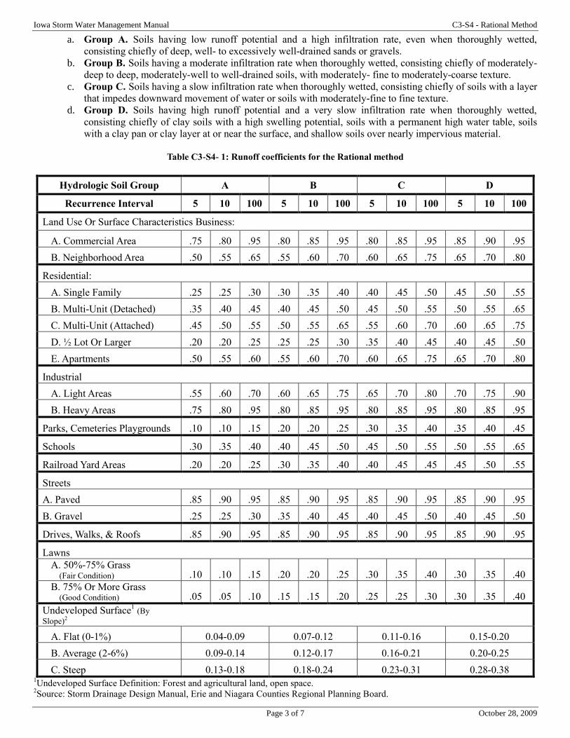
Iowa Storm Water Management Manual C3-S4 - Rational Method
Page 3 of 7 October 28, 2009
a. Group A. Soils having low runoff potential and a high infiltration rate, even when thoroughly wetted,
consisting chiefly of deep, well- to excessively well-drained sands or gravels.
b. Group B. Soils having a moderate infiltration rate when thoroughly wetted, consisting chiefly of moderately-
deep to deep, moderately-well to well-drained soils, with moderately- fine to moderately-coarse texture.
c. Group C. Soils having a slow infiltration rate when thoroughly wetted, consisting chiefly of soils with a layer
that impedes downward movement of water or soils with moderately-fine to fine texture.
d. Group D. Soils having high runoff potential and a very slow infiltration rate when thoroughly wetted,
consisting chiefly of clay soils with a high swelling potential, soils with a permanent high water table, soils
with a clay pan or clay layer at or near the surface, and shallow soils over nearly impervious material.
Table C3-S4- 1: Runoff coefficients for the Rational method
Hydrologic Soil Group A B C D
Recurrence Interval 5 10 100 5 10 100 5 10 100 5 10 100
Land Use Or Surface Characteristics Business:
A. Commercial Area .75 .80 .95 .80 .85 .95 .80 .85 .95 .85 .90 .95
B. Neighborhood Area .50 .55 .65 .55 .60 .70 .60 .65 .75 .65 .70 .80
Residential:
A. Single Family .25 .25 .30 .30 .35 .40 .40 .45 .50 .45 .50 .55
B. Multi-Unit (Detached) .35 .40 .45 .40 .45 .50 .45 .50 .55 .50 .55 .65
C. Multi-Unit (Attached) .45 .50 .55 .50 .55 .65 .55 .60 .70 .60 .65 .75
D. ½ Lot Or Larger .20 .20 .25 .25 .25 .30 .35 .40 .45 .40 .45 .50
E. Apartments .50 .55 .60 .55 .60 .70 .60 .65 .75 .65 .70 .80
Industrial
A. Light Areas .55 .60 .70 .60 .65 .75 .65 .70 .80 .70 .75 .90
B. Heavy Areas .75 .80 .95 .80 .85 .95 .80 .85 .95 .80 .85 .95
Parks, Cemeteries Playgrounds .10 .10 .15 .20 .20 .25 .30 .35 .40 .35 .40 .45
Schools .30 .35 .40 .40 .45 .50 .45 .50 .55 .50 .55 .65
Railroad Yard Areas .20 .20 .25 .30 .35 .40 .40 .45 .45 .45 .50 .55
Streets
A. Paved .85 .90 .95 .85 .90 .95 .85 .90 .95 .85 .90 .95
B. Gravel .25 .25 .30 .35 .40 .45 .40 .45 .50 .40 .45 .50
Drives, Walks, & Roofs .85 .90 .95 .85 .90 .95 .85 .90 .95 .85 .90 .95
Lawns
A. 50%-75% Grass (Fair Condition) .10 .10 .15 .20 .20 .25 .30 .35 .40 .30 .35 .40
B. 75% Or More Grass (Good Condition) .05 .05 .10 .15 .15 .20 .25 .25 .30 .30 .35 .40
Undeveloped Surface1 (By
Slope)2
A. Flat (0-1%) 0.04-0.09 0.07-0.12 0.11-0.16 0.15-0.20
B. Average (2-6%) 0.09-0.14 0.12-0.17 0.16-0.21 0.20-0.25
C. Steep 0.13-0.18 0.18-0.24 0.23-0.31 0.28-0.38 1Undeveloped Surface Definition: Forest and agricultural land, open space.
2Source: Storm Drainage Design Manual, Erie and Niagara Counties Regional Planning Board.
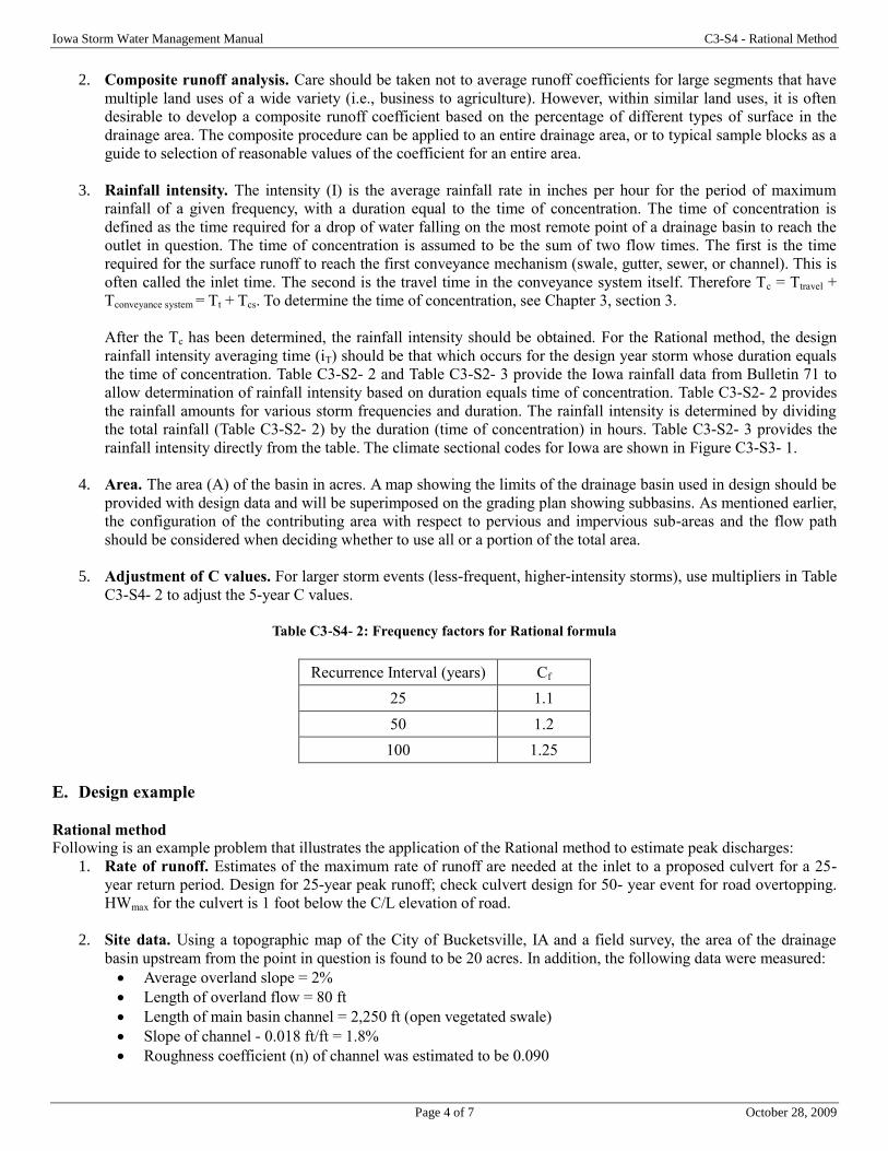
Iowa Storm Water Management Manual C3-S4 - Rational Method
Page 4 of 7 October 28, 2009
2. Composite runoff analysis. Care should be taken not to average runoff coefficients for large segments that have
multiple land uses of a wide variety (i.e., business to agriculture). However, within similar land uses, it is often
desirable to develop a composite runoff coefficient based on the percentage of different types of surface in the
drainage area. The composite procedure can be applied to an entire drainage area, or to typical sample blocks as a
guide to selection of reasonable values of the coefficient for an entire area.
3. Rainfall intensity. The intensity (I) is the average rainfall rate in inches per hour for the period of maximum
rainfall of a given frequency, with a duration equal to the time of concentration. The time of concentration is
defined as the time required for a drop of water falling on the most remote point of a drainage basin to reach the
outlet in question. The time of concentration is assumed to be the sum of two flow times. The first is the time
required for the surface runoff to reach the first conveyance mechanism (swale, gutter, sewer, or channel). This is
often called the inlet time. The second is the travel time in the conveyance system itself. Therefore Tc = Ttravel +
Tconveyance system = Tt + Tcs. To determine the time of concentration, see Chapter 3, section 3.
After the Tc has been determined, the rainfall intensity should be obtained. For the Rational method, the design
rainfall intensity averaging time (iT) should be that which occurs for the design year storm whose duration equals
the time of concentration. Table C3-S2- 2 and Table C3-S2- 3 provide the Iowa rainfall data from Bulletin 71 to
allow determination of rainfall intensity based on duration equals time of concentration. Table C3-S2- 2 provides
the rainfall amounts for various storm frequencies and duration. The rainfall intensity is determined by dividing
the total rainfall (Table C3-S2- 2) by the duration (time of concentration) in hours. Table C3-S2- 3 provides the
rainfall intensity directly from the table. The climate sectional codes for Iowa are shown in Figure C3-S3- 1.
4. Area. The area (A) of the basin in acres. A map showing the limits of the drainage basin used in design should be
provided with design data and will be superimposed on the grading plan showing subbasins. As mentioned earlier,
the configuration of the contributing area with respect to pervious and impervious sub-areas and the flow path
should be considered when deciding whether to use all or a portion of the total area.
5. Adjustment of C values. For larger storm events (less-frequent, higher-intensity storms), use multipliers in Table
C3-S4- 2 to adjust the 5-year C values.
Table C3-S4- 2: Frequency factors for Rational formula
Recurrence Interval (years) Cf
25 1.1
50 1.2
100 1.25
E. Design example
Rational method
Following is an example problem that illustrates the application of the Rational method to estimate peak discharges:
1. Rate of runoff. Estimates of the maximum rate of runoff are needed at the inlet to a proposed culvert for a 25-
year return period. Design for 25-year peak runoff; check culvert design for 50- year event for road overtopping.
HWmax for the culvert is 1 foot below the C/L elevation of road.
2. Site data. Using a topographic map of the City of Bucketsville, IA and a field survey, the area of the drainage
basin upstream from the point in question is found to be 20 acres. In addition, the following data were measured:
Average overland slope = 2%
Length of overland flow = 80 ft
Length of main basin channel = 2,250 ft (open vegetated swale)
Slope of channel - 0.018 ft/ft = 1.8%
Roughness coefficient (n) of channel was estimated to be 0.090
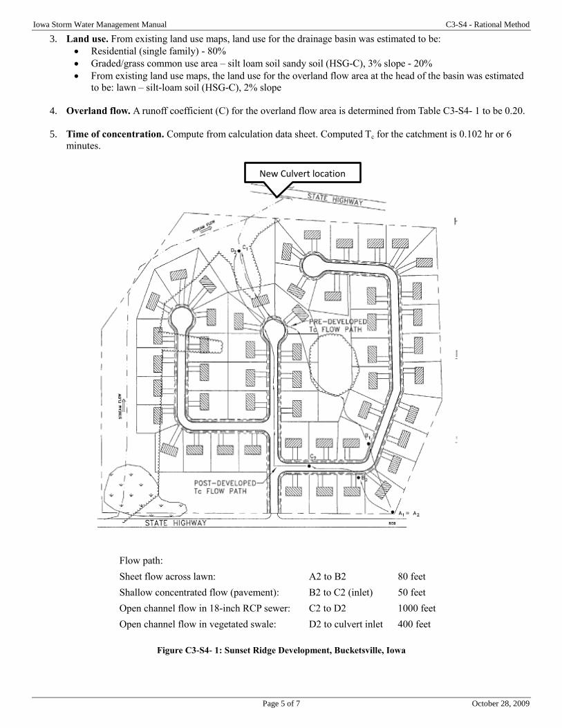
Iowa Storm Water Management Manual C3-S4 - Rational Method
Page 5 of 7 October 28, 2009
3. Land use. From existing land use maps, land use for the drainage basin was estimated to be:
Residential (single family) - 80%
Graded/grass common use area – silt loam soil sandy soil (HSG-C), 3% slope - 20%
From existing land use maps, the land use for the overland flow area at the head of the basin was estimated
to be: lawn – silt-loam soil (HSG-C), 2% slope
4. Overland flow. A runoff coefficient (C) for the overland flow area is determined from Table C3-S4- 1 to be 0.20.
5. Time of concentration. Compute from calculation data sheet. Computed Tc for the catchment is 0.102 hr or 6
minutes.
Flow path:
Sheet flow across lawn: A2 to B2 80 feet
Shallow concentrated flow (pavement): B2 to C2 (inlet) 50 feet
Open channel flow in 18-inch RCP sewer: C2 to D2 1000 feet
Open channel flow in vegetated swale: D2 to culvert inlet 400 feet
Figure C3-S4- 1: Sunset Ridge Development, Bucketsville, Iowa
New Culvert location
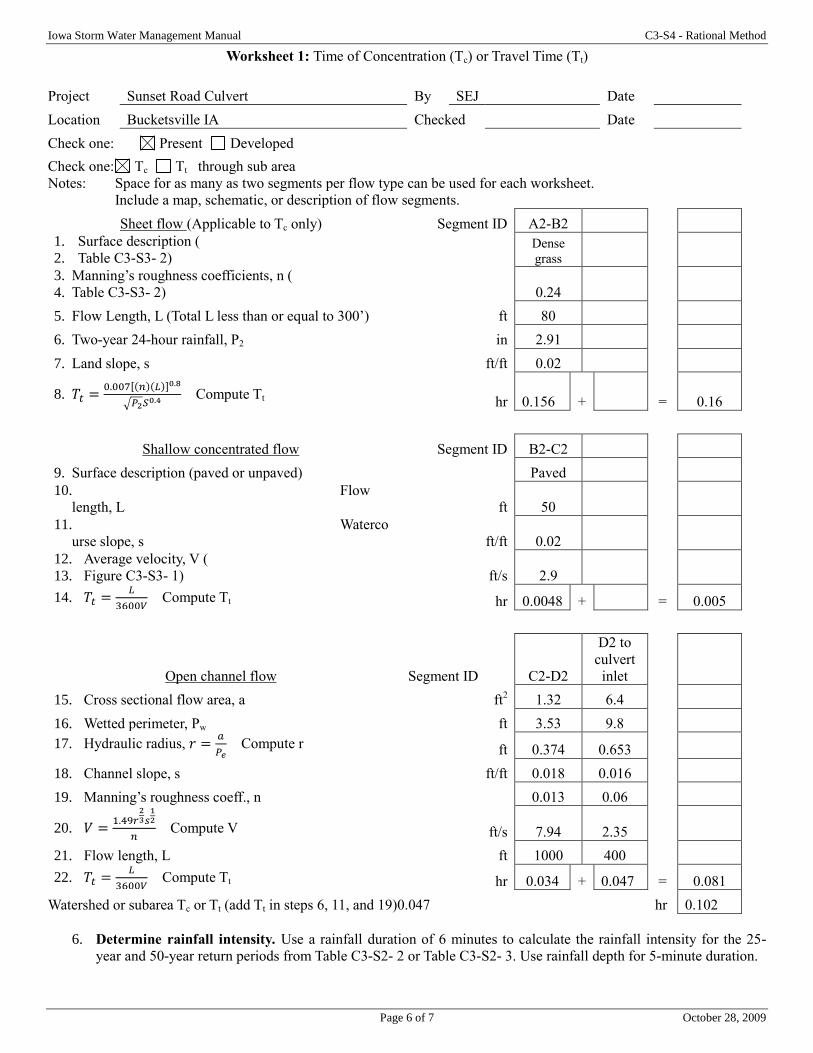
Iowa Storm Water Management Manual C3-S4 - Rational Method
Page 6 of 7 October 28, 2009
Worksheet 1: Time of Concentration (Tc) or Travel Time (Tt)
Project Sunset Road Culvert By SEJ Date
Location Bucketsville IA Checked Date
Check one: Present Developed
Check one: Tc Tt through sub area
Notes: Space for as many as two segments per flow type can be used for each worksheet.
Include a map, schematic, or description of flow segments.
Sheet flow (Applicable to Tc only) Segment ID A2-B2
1. Surface description (
2. Table C3-S3- 2)Dense
grass
3. Manning’s roughness coefficients, n (
4. Table C3-S3- 2) 0.24
5. Flow Length, L (Total L less than or equal to 300’) ft 80
6. Two-year 24-hour rainfall, P2 in 2.91
7. Land slope, s ft/ft 0.02
8. 𝑇𝑡 =0.007[(𝑛)(𝐿)]0.8
√𝑃2𝑆0.4 Compute Tt hr 0.156 + = 0.16
Shallow concentrated flow Segment ID B2-C2
9. Surface description (paved or unpaved) Paved
10. Flow
length, L ft 50
11. Waterco
urse slope, s ft/ft 0.02
12. Average velocity, V (
13. Figure C3-S3- 1) ft/s 2.9
14. 𝑇𝑡 =𝐿
3600𝑉 Compute Tt hr 0.0048 + = 0.005
Open channel flow Segment ID C2-D2
D2 to
culvert
inlet
15. Cross sectional flow area, a ft2 1.32 6.4
16. Wetted perimeter, Pw ft 3.53 9.8
17. Hydraulic radius, 𝑟 =𝑎
𝑃𝑒 Compute r ft 0.374 0.653
18. Channel slope, s ft/ft 0.018 0.016
19. Manning’s roughness coeff., n 0.013 0.06
20. 𝑉 =1.49𝑟
23𝑠
12
𝑛 Compute V ft/s 7.94 2.35
21. Flow length, L ft 1000 400
22. 𝑇𝑡 =𝐿
3600𝑉 Compute Tt hr 0.034 + 0.047 = 0.081
Watershed or subarea Tc or Tt (add Tt in steps 6, 11, and 19)0.047 hr 0.102
6. Determine rainfall intensity. Use a rainfall duration of 6 minutes to calculate the rainfall intensity for the 25-
year and 50-year return periods from Table C3-S2- 2 or Table C3-S2- 3. Use rainfall depth for 5-minute duration.
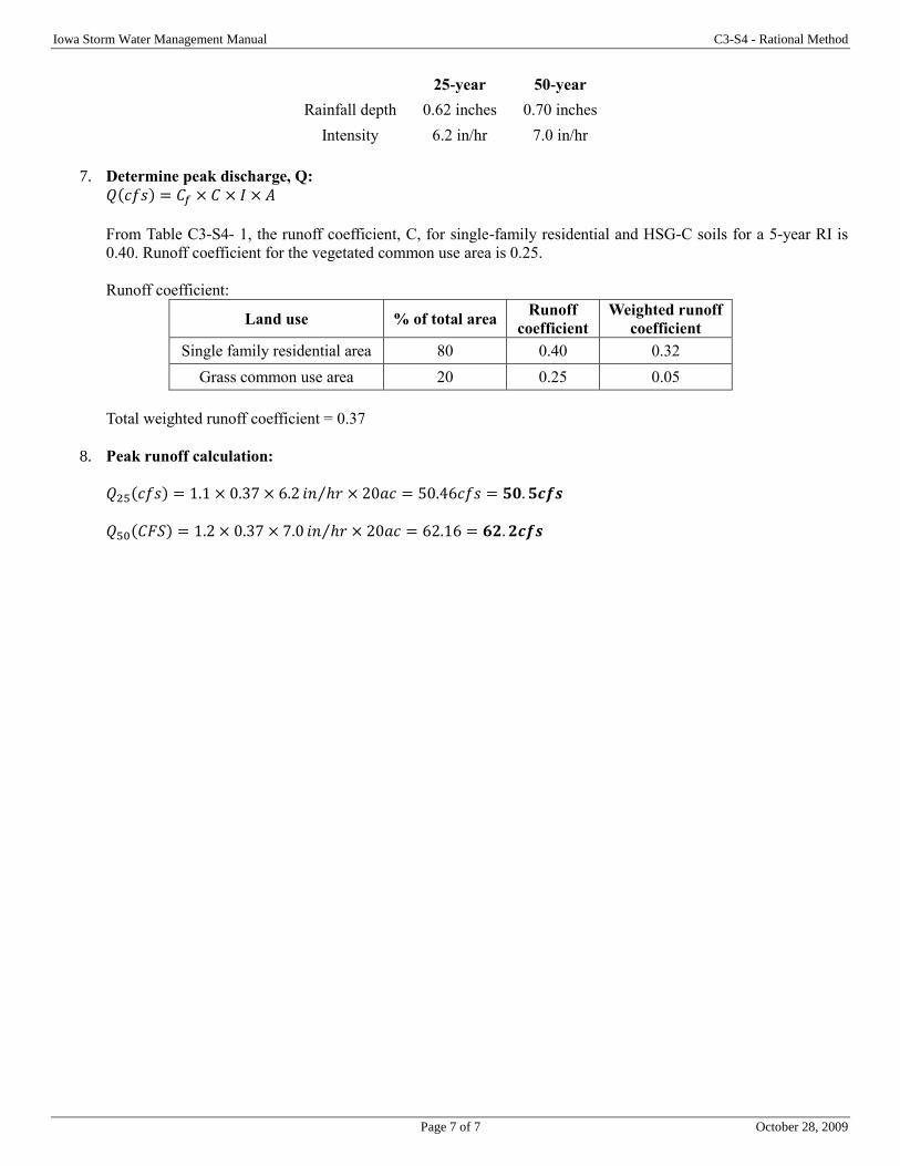
Iowa Storm Water Management Manual C3-S4 - Rational Method
Page 7 of 7 October 28, 2009
25-year 50-year
Rainfall depth 0.62 inches 0.70 inches
Intensity 6.2 in/hr 7.0 in/hr
7. Determine peak discharge, Q:
𝑄(𝑐𝑓𝑠) = 𝐶𝑓 × 𝐶 × 𝐼 × 𝐴
From Table C3-S4- 1, the runoff coefficient, C, for single-family residential and HSG-C soils for a 5-year RI is
0.40. Runoff coefficient for the vegetated common use area is 0.25.
Runoff coefficient:
Land use % of total area Runoff
coefficient
Weighted runoff
coefficient
Single family residential area 80 0.40 0.32
Grass common use area 20 0.25 0.05
Total weighted runoff coefficient = 0.37
8. Peak runoff calculation:
𝑄25(𝑐𝑓𝑠) = 1.1 × 0.37 × 6.2 𝑖𝑛 ℎ𝑟⁄ × 20𝑎𝑐 = 50.46𝑐𝑓𝑠 = 𝟓𝟎. 𝟓𝒄𝒇𝒔
𝑄50(𝐶𝐹𝑆) = 1.2 × 0.37 × 7.0 𝑖𝑛 ℎ𝑟⁄ × 20𝑎𝑐 = 62.16 = 𝟔𝟐. 𝟐𝒄𝒇𝒔

Page 1 of 12 October 28, 2009
Chapter 3- Section 5 NRCS TR-55 Methodology
A. Introduction
The Natural Resource Conservation Service (NRCS) hydrologic method requires basic data similar to the Rational
method: drainage area, a runoff factor, time of concentration, and rainfall. The NRCS approach, however, is more
sophisticated in that it also considers the time distribution of the rainfall, the initial rainfall losses to interception and
depression storage, and an infiltration rate that decreases during the course of a storm. Details of the methodology can be
found in the NRCS National Engineering Handbook, Section 4, Hydrology. A typical application of the NRCS method
includes the following basic steps:
1. Determination of curve numbers that represent different land uses within the drainage area.
2. Calculation of time of concentration to the study point.
3. Using the Type II or Type III rainfall distribution, total and excess rainfall amounts are determined. See
4. Figure C3-S5- 1 for the geographic boundaries for the different NRCS rainfall distributions.
5. Using the unit hydrograph approach, the hydrograph of direct runoff from the drainage basin can be developed.
The NRCS method can be used for both the estimation of stormwater runoff peak rates and the generation of hydrographs
for the routing of stormwater flows. The simplified method can be used for drainage areas up to 2,000 acres. The NRCS
method can be used for most design applications, including storage facilities, outlet structures, storm drain systems,
culverts, small drainage ditches, open channels, and energy dissipaters.
B. Equations and concepts
The hydrograph of outflow from a drainage basin is the sum of the elemental hydrographs from all the sub-areas of the
basin, modified by the effects of transit time through the basin and storage in the stream channels. Since the physical
characteristics of the basin (shape, size, and slope) are constant, the unit hydrograph approach assumes that there is
considerable similarity in the shape of hydrographs from storms of similar rainfall characteristics. Thus, the unit
hydrograph is a typical hydrograph for the basin with a runoff volume under the hydrograph equal to 1 inch from a storm
of specified duration. For a storm of the same duration, but with a different amount of runoff, the hydrograph of direct
runoff can be expected to have the same time base as the unit hydrograph and ordinates of flow proportional to the runoff
volume. Therefore, a storm that produces 2 inches of runoff would have a hydrograph with a flow equal to twice the flow
of the unit hydrograph. With 0.5 inches of runoff, the flow of the hydrograph would be one-half of the flow of the unit
hydrograph.
The following discussion outlines the equations and basin concepts used in the NRCS method:
1. Drainage area. The drainage area of a watershed is determined from topographic maps and field surveys. For
large drainage areas, it might be necessary to divide the area into sub-drainage areas to account for major land use
changes, obtain analysis results at different points within the drainage area, combine hydrographs from different
subbasins as applicable, and/or route flows to points of interest.
2. Rainfall. The NRCS method applicable to the State of Iowa is based on a storm event that has a Type II time
distribution. These distributions are used to distribute the 24-hour volume of rainfall for the different storm
frequencies (Figure C3-S5- 1).
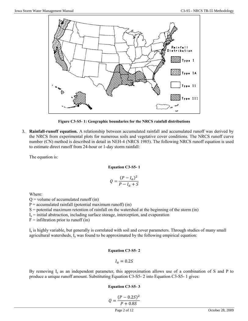
Iowa Storm Water Management Manual C3-S5 - NRCS TR-55 Methodology
Page 2 of 12 October 28, 2009
Figure C3-S5- 1: Geographic boundaries for the NRCS rainfall distributions
3. Rainfall-runoff equation. A relationship between accumulated rainfall and accumulated runoff was derived by
the NRCS from experimental plots for numerous soils and vegetative cover conditions. The NRCS runoff curve
number (CN) method is described in detail in NEH-4 (NRCS 1985). The following NRCS runoff equation is used
to estimate direct runoff from 24-hour or 1-day storm rainfall:
The equation is:
Equation C3-S5- 1
𝑄 =(𝑃 − 𝐼𝑎)2
𝑃 − 𝐼𝑎 + 𝑆
Where:
Q = volume of accumulated runoff (in)
P = accumulated rainfall (potential maximum runoff) (in)
S = potential maximum retention of rainfall on the watershed at the beginning of the storm (in)
Ia = initial abstraction, including surface storage, interception, and evaporation
F = infiltration prior to runoff (in)
Ia is highly variable, but generally is correlated with soil and cover parameters. Through studies of many small
agricultural watersheds, Ia was found to be approximated by the following empirical equation:
Equation C3-S5- 2
𝐼𝑎 = 0.2𝑆
By removing Ia as an independent parameter, this approximation allows use of a combination of S and P to
produce a unique runoff amount. Substituting Equation C3-S5- 2 into Equation C3-S5- 1 gives:
Equation C3-S5- 3
𝑄 =(𝑃 − 0.2𝑆)2
𝑃 + 0.8𝑆
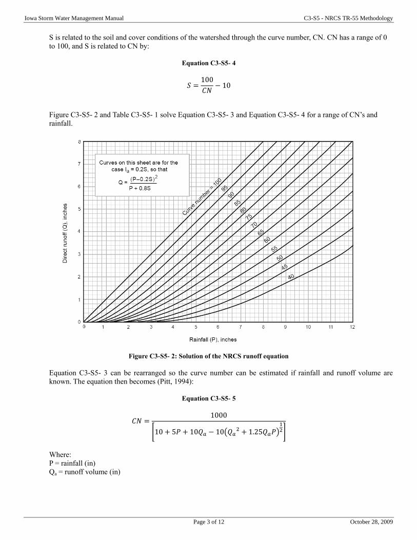
Iowa Storm Water Management Manual C3-S5 - NRCS TR-55 Methodology
Page 3 of 12 October 28, 2009
S is related to the soil and cover conditions of the watershed through the curve number, CN. CN has a range of 0
to 100, and S is related to CN by:
Equation C3-S5- 4
𝑆 =100
𝐶𝑁− 10
Figure C3-S5- 2 and Table C3-S5- 1 solve Equation C3-S5- 3 and Equation C3-S5- 4 for a range of CN’s and
rainfall.
Figure C3-S5- 2: Solution of the NRCS runoff equation
Equation C3-S5- 3 can be rearranged so the curve number can be estimated if rainfall and runoff volume are
known. The equation then becomes (Pitt, 1994):
Equation C3-S5- 5
𝐶𝑁 =1000
[10 + 5𝑃 + 10𝑄𝑎 − 10(𝑄𝑎2 + 1.25𝑄𝑎𝑃)
12]
Where:
P = rainfall (in)
Qa = runoff volume (in)
Iowa Storm Water Management Manual C3-S5 - NRCS TR-55 Methodology
Page 4 of 12 October 28, 2009
Table C3-S5- 1: Runoff depth for selected CN’s and rainfall amounts1
Runoff depth for curve number of:
Rainfal
l 40 45 50 55 60 65 70 75 80 85 90 95 98
1.0 0.00 0.00 0.00 0.00 0.00 0.00 0.00 0.03 0.08 0.17 0.32 0.56 0.79
1.2 .00 .00 .00 .00 .00 .00 .03 .07 .10 .27 .46 .74 .99
1.4 .00 .00 .00 .00 .00 .02 .06 .13 .24 .39 .61 .92 1.18
1.6 .00 .00 .00 .00 .01 .05 .11 .20 .34 .52 .76 1.11 1.38
1.8 .00 .00 .00 .00 .03 .09 .17 .29 .44 .65 .93 1.29 1.58
2.0 .00 .00 .00 .02 .06 .14 .24 .38 .56 .80 1.09 1.48 1.77
2.5 .00 .00 .02 .08 .17 .30 .46 .65 .89 1.18 1.53 1.96 2.27
3.0 .00 .02 .09 .19 .33 .51 .71 .96 1.25 1.59 1.98 2.45 2.77
3.5 .02 .08 .20 .35 .53 .75 1.01 1.30 1.64 2.02 2.45 2.94 3.27
4.0 .06 .18 .33 .53 .76 1.03 1.33 1.67 2.04 2.46 2.92 3.43 3.77
4.5 .14 .30 .50 .74 1.02 1.33 1.67 2.05 2.46 2.91 3.40 3.92 4.26
5.0 .24 .44 .69 .98 1.30 1.65 2.04 2.45 2.89 3.37 3.88 4.42 4.76
6.0 .50 .80 1.14 1.52 1.92 2.35 2.81 3.28 3.78 4.30 4.85 5.41 5.76
7.0 .84 1.24 1.68 2.12 2.60 3.10 3.62 4.15 4.69 5.25 5.82 6.41 6.76
8.0 1.25 1.74 2.25 2.78 3.33 3.89 4.46 5.04 5.63 6.21 6.81 7.40 7.76
9.0 1.71 2.29 2.88 3.49 4.10 4.72 5.33 5.95 6.57 7.18 7.79 8.40 8.76
10.0 2.23 2.89 3.56 4.23 4.90 5.56 6.22 6.88 7.52 8.16 8.78 9.40 9.76
11.0 2.78 3.52 4.26 5.00 5.72 6.43 7.13 7.81 8.48 9.13 9.77 10.39 10.76
12.0 3.38 4.19 5.00 5.79 6.56 7.32 8.05 8.76 9.45 10.11 10.76 11.39 11.76
13.0 4.00 4.89 5.76 6.61 7.42 8.21 8.98 9.71 10.42 11.10 11.76 12.39 12.76
14.0 4.65 5.62 6.55 7.44 8.30 9.12 9.91 10.67 11.39 12.08 12.75 13.39 13.76
15.0 5.33 6.36 7.35 8.29 9.19 10.04 10.85 11.63 12.37 13.07 13.74 14.39 14.76 1Interpolate the values shown to obtain runoff depths for CNs or rainfall amounts not shown.
C. Runoff factor
The principal physical watershed characteristics affecting the relationship between rainfall and runoff are land use, land
treatment, soil types, and land slope. The NRCS method uses a combination of soil conditions and land uses (ground
cover) to assign a runoff factor to an area. These runoff factors, called runoff curve numbers (CN), indicate the runoff
potential of an area. The higher the CN, the higher the runoff potential. Soil properties influence the relationship between
runoff and rainfall since soils have differing rates of infiltration. Based on infiltration rates, the NRCS has divided soils
into four hydrologic soil groups:
1. Group A soils. Have a low runoff potential due to high infiltration rates. These soils consist primarily of deep,
well-drained sands and gravels.
2. Group B soils. Have a moderately low runoff potential due to moderate infiltration rates. These soils consist
primarily of moderately deep to deep, moderately well- to well-drained soils with moderately fine to moderately
coarse textures.
3. Group C soils. Have a moderately high runoff potential due to slow infiltration rates. These soils consist
primarily of soils in which a layer exists near the surface that impedes the downward movement of water or soils
with moderately fine to fine texture.
4. Group D soils. Have a high runoff potential due to very slow infiltration rates. These soils consist primarily of
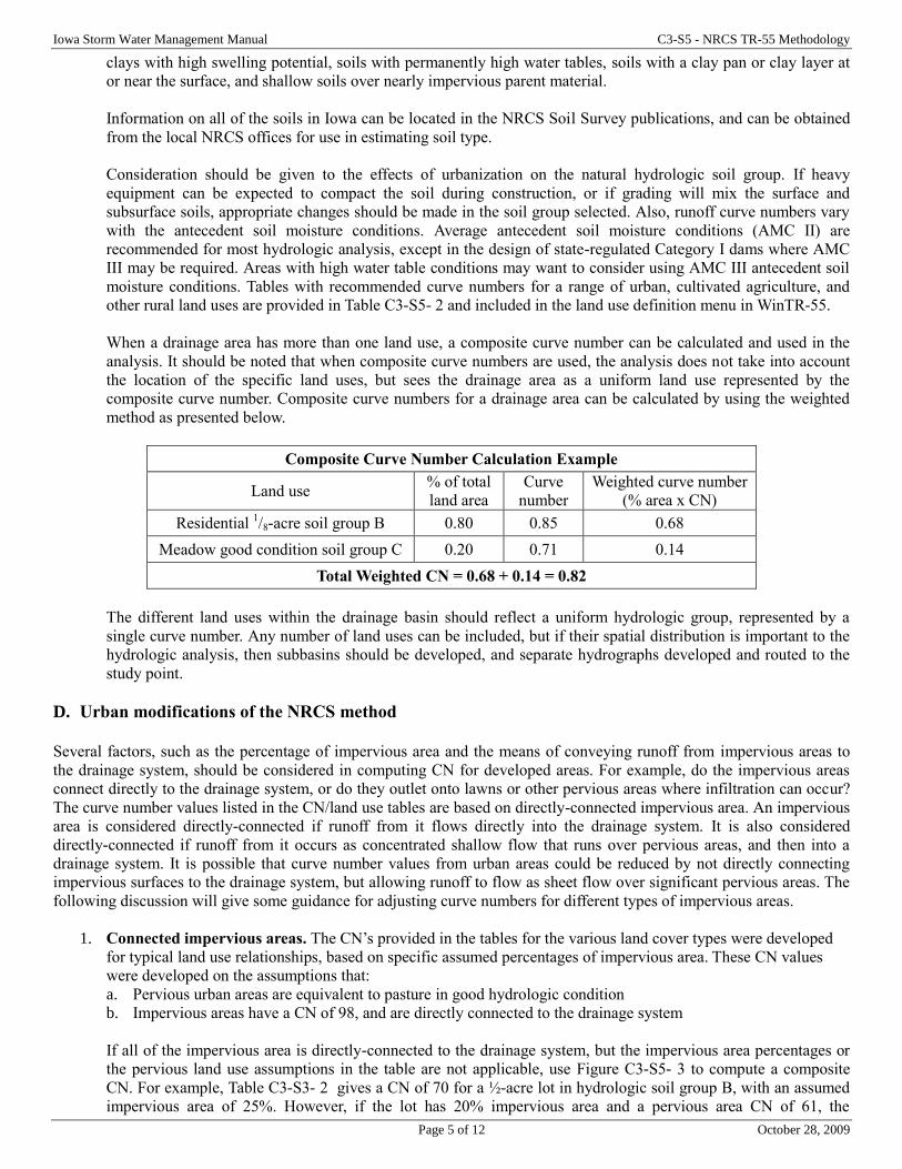
Iowa Storm Water Management Manual C3-S5 - NRCS TR-55 Methodology
Page 5 of 12 October 28, 2009
clays with high swelling potential, soils with permanently high water tables, soils with a clay pan or clay layer at
or near the surface, and shallow soils over nearly impervious parent material.
Information on all of the soils in Iowa can be located in the NRCS Soil Survey publications, and can be obtained
from the local NRCS offices for use in estimating soil type.
Consideration should be given to the effects of urbanization on the natural hydrologic soil group. If heavy
equipment can be expected to compact the soil during construction, or if grading will mix the surface and
subsurface soils, appropriate changes should be made in the soil group selected. Also, runoff curve numbers vary
with the antecedent soil moisture conditions. Average antecedent soil moisture conditions (AMC II) are
recommended for most hydrologic analysis, except in the design of state-regulated Category I dams where AMC
III may be required. Areas with high water table conditions may want to consider using AMC III antecedent soil
moisture conditions. Tables with recommended curve numbers for a range of urban, cultivated agriculture, and
other rural land uses are provided in Table C3-S5- 2 and included in the land use definition menu in WinTR-55.
When a drainage area has more than one land use, a composite curve number can be calculated and used in the
analysis. It should be noted that when composite curve numbers are used, the analysis does not take into account
the location of the specific land uses, but sees the drainage area as a uniform land use represented by the
composite curve number. Composite curve numbers for a drainage area can be calculated by using the weighted
method as presented below.
Composite Curve Number Calculation Example
Land use % of total
land area
Curve
number
Weighted curve number
(% area x CN)
Residential 1/8-acre soil group B 0.80 0.85 0.68
Meadow good condition soil group C 0.20 0.71 0.14
Total Weighted CN = 0.68 + 0.14 = 0.82
The different land uses within the drainage basin should reflect a uniform hydrologic group, represented by a
single curve number. Any number of land uses can be included, but if their spatial distribution is important to the
hydrologic analysis, then subbasins should be developed, and separate hydrographs developed and routed to the
study point.
D. Urban modifications of the NRCS method
Several factors, such as the percentage of impervious area and the means of conveying runoff from impervious areas to
the drainage system, should be considered in computing CN for developed areas. For example, do the impervious areas
connect directly to the drainage system, or do they outlet onto lawns or other pervious areas where infiltration can occur?
The curve number values listed in the CN/land use tables are based on directly-connected impervious area. An impervious
area is considered directly-connected if runoff from it flows directly into the drainage system. It is also considered
directly-connected if runoff from it occurs as concentrated shallow flow that runs over pervious areas, and then into a
drainage system. It is possible that curve number values from urban areas could be reduced by not directly connecting
impervious surfaces to the drainage system, but allowing runoff to flow as sheet flow over significant pervious areas. The
following discussion will give some guidance for adjusting curve numbers for different types of impervious areas.
1. Connected impervious areas. The CN’s provided in the tables for the various land cover types were developed
for typical land use relationships, based on specific assumed percentages of impervious area. These CN values
were developed on the assumptions that:
a. Pervious urban areas are equivalent to pasture in good hydrologic condition
b. Impervious areas have a CN of 98, and are directly connected to the drainage system
If all of the impervious area is directly-connected to the drainage system, but the impervious area percentages or
the pervious land use assumptions in the table are not applicable, use Figure C3-S5- 3 to compute a composite
CN. For example, Table C3-S3- 2 gives a CN of 70 for a ½-acre lot in hydrologic soil group B, with an assumed
impervious area of 25%. However, if the lot has 20% impervious area and a pervious area CN of 61, the

Iowa Storm Water Management Manual C3-S5 - NRCS TR-55 Methodology
Page 6 of 12 October 28, 2009
composite CN obtained from Figure C3-S5- 3 is 68. The CN difference between 70 and 68 reflects the difference
in percent impervious area. In the current version of WinTR-55, the user may do this conversion quickly though
the interactive menu in the program. WinTR-55 will also allow the user to create custom CN’s based on the site
imperviousness and/or other site conditions.
Table C3-S5- 2: NRCS runoff curve numbers (CN) for selected urban land use1
Cover description Curve numbers for
hydrologic soil group
Cover type and hydrologic condition
Average
imperviou
s area2
A B C D
Fully developed urban areas (vegetation established)
Open space (lawns, parks, golf courses, cemeteries, etc)3:
Poor condition (grass cover <50%) 68 79 86 89
Fair condition (grass cover 50% to 75%) 49 69 79 84
Good condition (grass cover >75%) 39 61 74 80
Impervious areas:
Paved parking lots, roofs, driveways, etc (excluding ROW) 98 98 98 98
Streets and roads:
Paved: curbs and storm sewers (excluding ROW) 98 98 98 98
Paved: open ditches (including ROW) 83 89 92 93
Gravel (including ROW) 76 85 89 91
Dirt (including ROW) 72 82 87 89
Western desert urban areas:
Natural desert landscaping (pervious areas only)4 63 77 85 88
Artificial desert landscaping (impervious weed barrier, desert shrub
with 1-2 inch sand or gravel mulch and basin borders) 96 96 96 96
Urban districts:
Commercial and business 85 89 92 94 95
Industrial 72 81 88 91 93
Residential districts by average lot size:
⅛ acre or less (town houses) 65 77 85 90 92
¼ acre 38 61 75 83 87
⅛ acre 30 57 72 81 86
½ acre 25 54 70 80 85
1 acre 20 51 68 79 84
2 acres 12 46 65 77 82
Developing urban areas
Newly graded areas (pervious areas only, no vegetation)5 77 86 91 94
Idle lands (CN’s are determined using cover types similar to those in Table C3-
S5- 3 1Average runoff condition and Ia=0.2S.
2The average percent impervious area shown was used to develop the composite CN’s. Other assumptions are as follows:
impervious areas are directly connected to the drainage system, impervious areas have a CN of 98, and pervious areas are
considered equivalent to open space in good hydrologic condition. CN’s for other combinations of conditions pay be
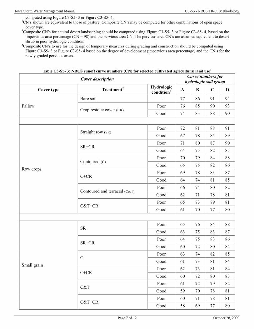
Iowa Storm Water Management Manual C3-S5 - NRCS TR-55 Methodology
Page 7 of 12 October 28, 2009
computed using Figure C3-S5- 3 or Figure C3-S5- 4. 3CN’s shown are equivalent to those of pasture. Composite CN’s may be computed for other combinations of open space
cover type. 4Composite CN’s for natural desert landscaping should be computed using Figure C3-S5- 3 or Figure C3-S5- 4, based on the
impervious area percentage (CN = 98) and the pervious area CN. The pervious area CN’s are assumed equivalent to desert
shrub in poor hydrologic condition. 5Composite CN’s to use for the design of temporary measures during grading and construction should be computed using
Figure C3-S5- 3 or Figure C3-S5- 4 based on the degree of development (impervious area percentage) and the CN’s for the
newly graded pervious areas.
Table C3-S5- 3: NRCS runoff curve numbers (CN) for selected cultivated agricultural land use1
Cover description Curve numbers for
hydrologic soil group
Cover type Treatment2
Hydrologic
condition3
A B C D
Fallow
Bare soil -- 77 86 91 94
Crop residue cover (CR) Poor 76 85 90 93
Good 74 83 88 90
Row crops
Straight row (SR) Poor 72 81 88 91
Good 67 78 85 89
SR+CR Poor 71 80 87 90
Good 64 75 82 85
Contoured (C) Poor 70 79 84 88
Good 65 75 82 86
C+CR Poor 69 78 83 87
Good 64 74 81 85
Contoured and terraced (C&T) Poor 66 74 80 82
Good 62 71 78 81
C&T+CR Poor 65 73 79 81
Good 61 70 77 80
Small grain
SR Poor 65 76 84 88
Good 63 75 83 87
SR+CR Poor 64 75 83 86
Good 60 72 80 84
C Poor 63 74 82 85
Good 61 73 81 84
C+CR Poor 62 73 81 84
Good 60 72 80 83
C&T Poor 61 72 79 82
Good 59 70 78 81
C&T+CR Poor 60 71 78 81
Good 58 69 77 80

Iowa Storm Water Management Manual C3-S5 - NRCS TR-55 Methodology
Page 8 of 12 October 28, 2009
Close- seeded or broadcast
legumes or rotation meadow
SR Poor 66 77 85 89
Good 58 72 81 85
C Poor 64 75 83 85
Good 55 69 78 83
C&T Poor 63 73 80 83
Good 51 67 76 80 1Average runoff condition and Ia=0.2S.
2Crop residue cover applies only if residue is on at least 5% of the surface throughout the year.
3Hydraulic condition is based on combination factors that affect infiltration and runoff, including (a) density and canopy of
vegetative areas, (b) amount of year-round cover, (c) amount of grass or close- seeded legumes, (d) percent of residue cover
on the land surface (good 20%), and (e) degree of surface roughness.
Poor: factors impair infiltration and tend to increase runoff.
Good: factors encourage average and better than average infiltration and tend to decrease runoff.
Table C3-S5- 4: NRCS runoff curve numbers (CN) for other agricultural land use1
Cover description Curve numbers for
hydrologic soil group
Cover type
Hydrologi
c
condition
A B C D
Pasture, grassland, or range – continuous forage for grazing2
Poor 68 79 86 89
Fair 49 69 79 84
Good 39 61 74 80
Meadow – continuous grass, protected from grazing and generally
mowed for hay -- 30 58 71 78
Brush – brush-weed-grass mixture with brush the major element3
Poor 48 67 77 83
Fair 35 56 70 77
Good 304
48 65 73
Woods – grass combination (orchard or tree farm)5
Poor 57 73 82 86
Fair 43 65 76 82
Good 32 58 72 79
Woods6
Poor 45 66 77 83
Fair 36 60 73 79
Good 304 55 70 77
Farmsteads – buildings, lanes, driveways, and surrounding lots -- 59 74 82 86 1Average runoff condition and Ia=0.2S.
2Poor: <50% ground cover or heavily grazed with no mulch.
Fair: 50% to 75% ground cover and not heavily grazed.
Good: >75% ground cover and lightly or only occasionally grazed. 3Poor: <50% ground cover.
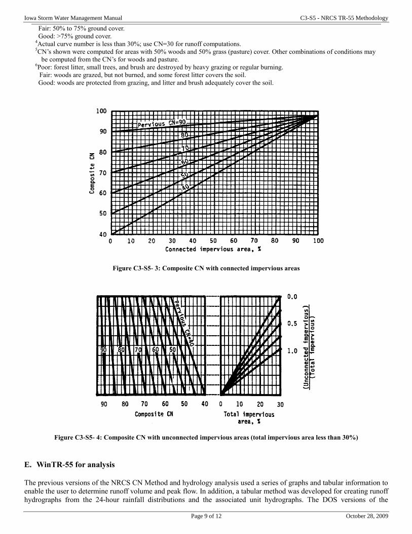
Iowa Storm Water Management Manual C3-S5 - NRCS TR-55 Methodology
Page 9 of 12 October 28, 2009
Fair: 50% to 75% ground cover.
Good: >75% ground cover. 4Actual curve number is less than 30%; use CN=30 for runoff computations.
5CN’s shown were computed for areas with 50% woods and 50% grass (pasture) cover. Other combinations of conditions may
be computed from the CN’s for woods and pasture. 6Poor: forest litter, small trees, and brush are destroyed by heavy grazing or regular burning.
Fair: woods are grazed, but not burned, and some forest litter covers the soil.
Good: woods are protected from grazing, and litter and brush adequately cover the soil.
Figure C3-S5- 3: Composite CN with connected impervious areas
Figure C3-S5- 4: Composite CN with unconnected impervious areas (total impervious area less than 30%)
E. WinTR-55 for analysis
The previous versions of the NRCS CN Method and hydrology analysis used a series of graphs and tabular information to
enable the user to determine runoff volume and peak flow. In addition, a tabular method was developed for creating runoff
hydrographs from the 24-hour rainfall distributions and the associated unit hydrographs. The DOS versions of the
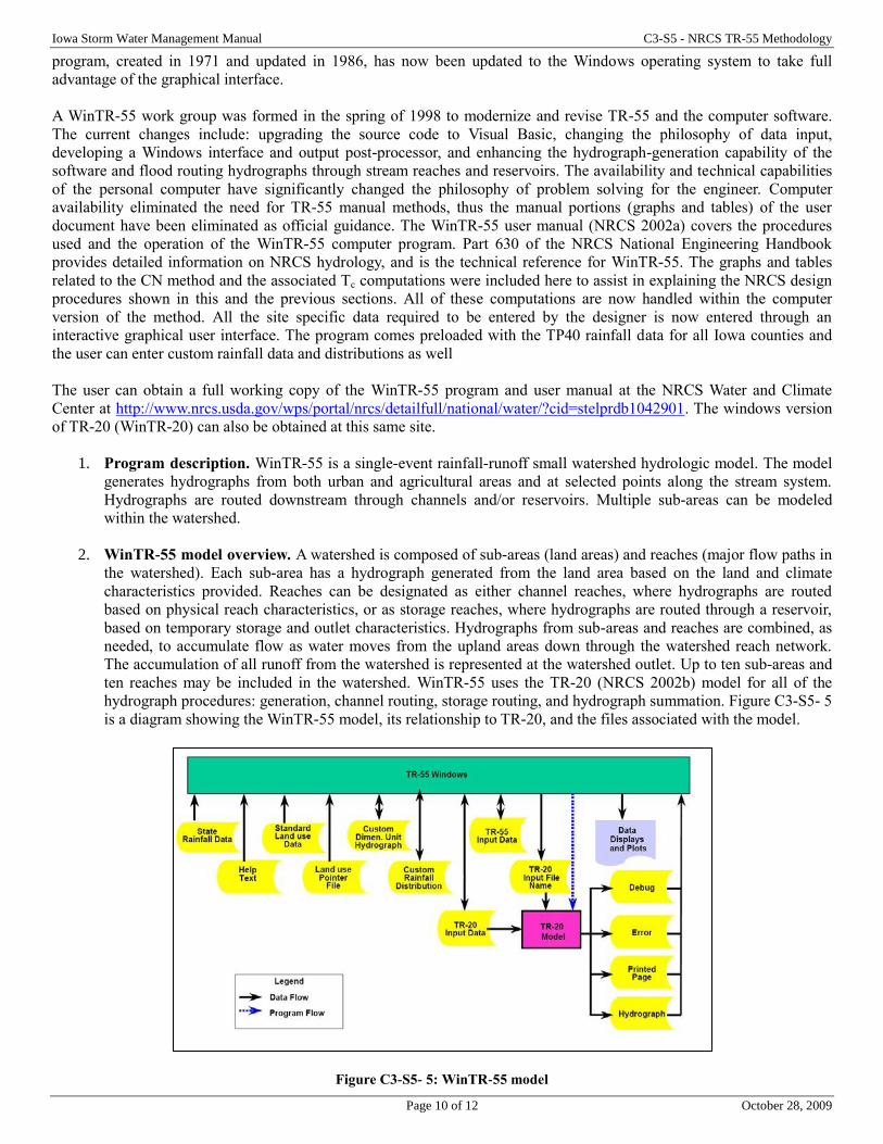
Iowa Storm Water Management Manual C3-S5 - NRCS TR-55 Methodology
Page 10 of 12 October 28, 2009
program, created in 1971 and updated in 1986, has now been updated to the Windows operating system to take full
advantage of the graphical interface.
A WinTR-55 work group was formed in the spring of 1998 to modernize and revise TR-55 and the computer software.
The current changes include: upgrading the source code to Visual Basic, changing the philosophy of data input,
developing a Windows interface and output post-processor, and enhancing the hydrograph-generation capability of the
software and flood routing hydrographs through stream reaches and reservoirs. The availability and technical capabilities
of the personal computer have significantly changed the philosophy of problem solving for the engineer. Computer
availability eliminated the need for TR-55 manual methods, thus the manual portions (graphs and tables) of the user
document have been eliminated as official guidance. The WinTR-55 user manual (NRCS 2002a) covers the procedures
used and the operation of the WinTR-55 computer program. Part 630 of the NRCS National Engineering Handbook
provides detailed information on NRCS hydrology, and is the technical reference for WinTR-55. The graphs and tables
related to the CN method and the associated Tc computations were included here to assist in explaining the NRCS design
procedures shown in this and the previous sections. All of these computations are now handled within the computer
version of the method. All the site specific data required to be entered by the designer is now entered through an
interactive graphical user interface. The program comes preloaded with the TP40 rainfall data for all Iowa counties and
the user can enter custom rainfall data and distributions as well
The user can obtain a full working copy of the WinTR-55 program and user manual at the NRCS Water and Climate
Center at http://www.nrcs.usda.gov/wps/portal/nrcs/detailfull/national/water/?cid=stelprdb1042901. The windows version
of TR-20 (WinTR-20) can also be obtained at this same site.
1. Program description. WinTR-55 is a single-event rainfall-runoff small watershed hydrologic model. The model
generates hydrographs from both urban and agricultural areas and at selected points along the stream system.
Hydrographs are routed downstream through channels and/or reservoirs. Multiple sub-areas can be modeled
within the watershed.
2. WinTR-55 model overview. A watershed is composed of sub-areas (land areas) and reaches (major flow paths in
the watershed). Each sub-area has a hydrograph generated from the land area based on the land and climate
characteristics provided. Reaches can be designated as either channel reaches, where hydrographs are routed
based on physical reach characteristics, or as storage reaches, where hydrographs are routed through a reservoir,
based on temporary storage and outlet characteristics. Hydrographs from sub-areas and reaches are combined, as
needed, to accumulate flow as water moves from the upland areas down through the watershed reach network.
The accumulation of all runoff from the watershed is represented at the watershed outlet. Up to ten sub-areas and
ten reaches may be included in the watershed. WinTR-55 uses the TR-20 (NRCS 2002b) model for all of the
hydrograph procedures: generation, channel routing, storage routing, and hydrograph summation. Figure C3-S5- 5
is a diagram showing the WinTR-55 model, its relationship to TR-20, and the files associated with the model.
Figure C3-S5- 5: WinTR-55 model
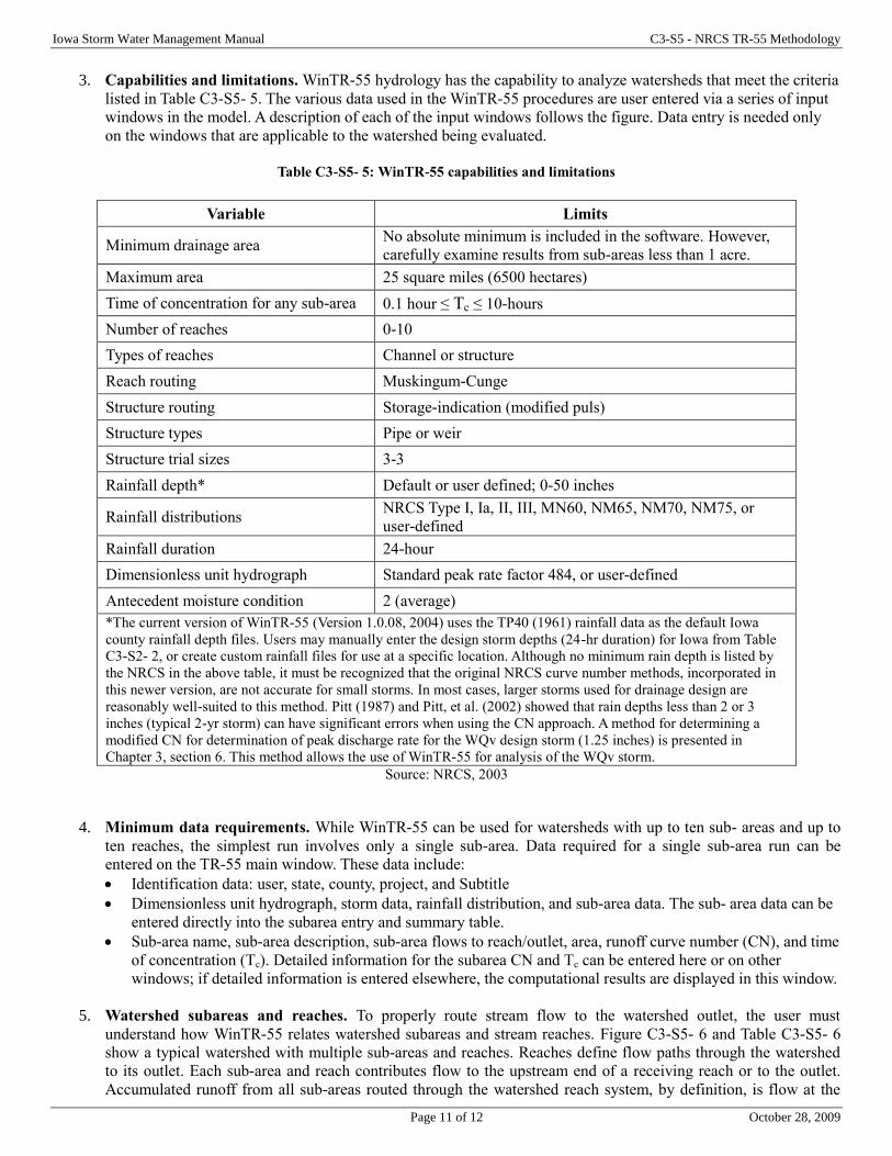
Iowa Storm Water Management Manual C3-S5 - NRCS TR-55 Methodology
Page 11 of 12 October 28, 2009
3. Capabilities and limitations. WinTR-55 hydrology has the capability to analyze watersheds that meet the criteria
listed in Table C3-S5- 5. The various data used in the WinTR-55 procedures are user entered via a series of input
windows in the model. A description of each of the input windows follows the figure. Data entry is needed only
on the windows that are applicable to the watershed being evaluated.
Table C3-S5- 5: WinTR-55 capabilities and limitations
Variable Limits
Minimum drainage area No absolute minimum is included in the software. However,
carefully examine results from sub-areas less than 1 acre.
Maximum area 25 square miles (6500 hectares)
Time of concentration for any sub-area 0.1 hour ≤ Tc ≤ 10-hours
Number of reaches 0-10
Types of reaches Channel or structure
Reach routing Muskingum-Cunge
Structure routing Storage-indication (modified puls)
Structure types Pipe or weir
Structure trial sizes 3-3
Rainfall depth* Default or user defined; 0-50 inches
Rainfall distributions NRCS Type I, Ia, II, III, MN60, NM65, NM70, NM75, or
user-defined
Rainfall duration 24-hour
Dimensionless unit hydrograph Standard peak rate factor 484, or user-defined
Antecedent moisture condition 2 (average)
*The current version of WinTR-55 (Version 1.0.08, 2004) uses the TP40 (1961) rainfall data as the default Iowa
county rainfall depth files. Users may manually enter the design storm depths (24-hr duration) for Iowa from Table
C3-S2- 2, or create custom rainfall files for use at a specific location. Although no minimum rain depth is listed by
the NRCS in the above table, it must be recognized that the original NRCS curve number methods, incorporated in
this newer version, are not accurate for small storms. In most cases, larger storms used for drainage design are
reasonably well-suited to this method. Pitt (1987) and Pitt, et al. (2002) showed that rain depths less than 2 or 3
inches (typical 2-yr storm) can have significant errors when using the CN approach. A method for determining a
modified CN for determination of peak discharge rate for the WQv design storm (1.25 inches) is presented in
Chapter 3, section 6. This method allows the use of WinTR-55 for analysis of the WQv storm. Source: NRCS, 2003
4. Minimum data requirements. While WinTR-55 can be used for watersheds with up to ten sub- areas and up to
ten reaches, the simplest run involves only a single sub-area. Data required for a single sub-area run can be
entered on the TR-55 main window. These data include:
Identification data: user, state, county, project, and Subtitle
Dimensionless unit hydrograph, storm data, rainfall distribution, and sub-area data. The sub- area data can be
entered directly into the subarea entry and summary table.
Sub-area name, sub-area description, sub-area flows to reach/outlet, area, runoff curve number (CN), and time
of concentration (Tc). Detailed information for the subarea CN and Tc can be entered here or on other
windows; if detailed information is entered elsewhere, the computational results are displayed in this window.
5. Watershed subareas and reaches. To properly route stream flow to the watershed outlet, the user must
understand how WinTR-55 relates watershed subareas and stream reaches. Figure C3-S5- 6 and Table C3-S5- 6
show a typical watershed with multiple sub-areas and reaches. Reaches define flow paths through the watershed
to its outlet. Each sub-area and reach contributes flow to the upstream end of a receiving reach or to the outlet.
Accumulated runoff from all sub-areas routed through the watershed reach system, by definition, is flow at the
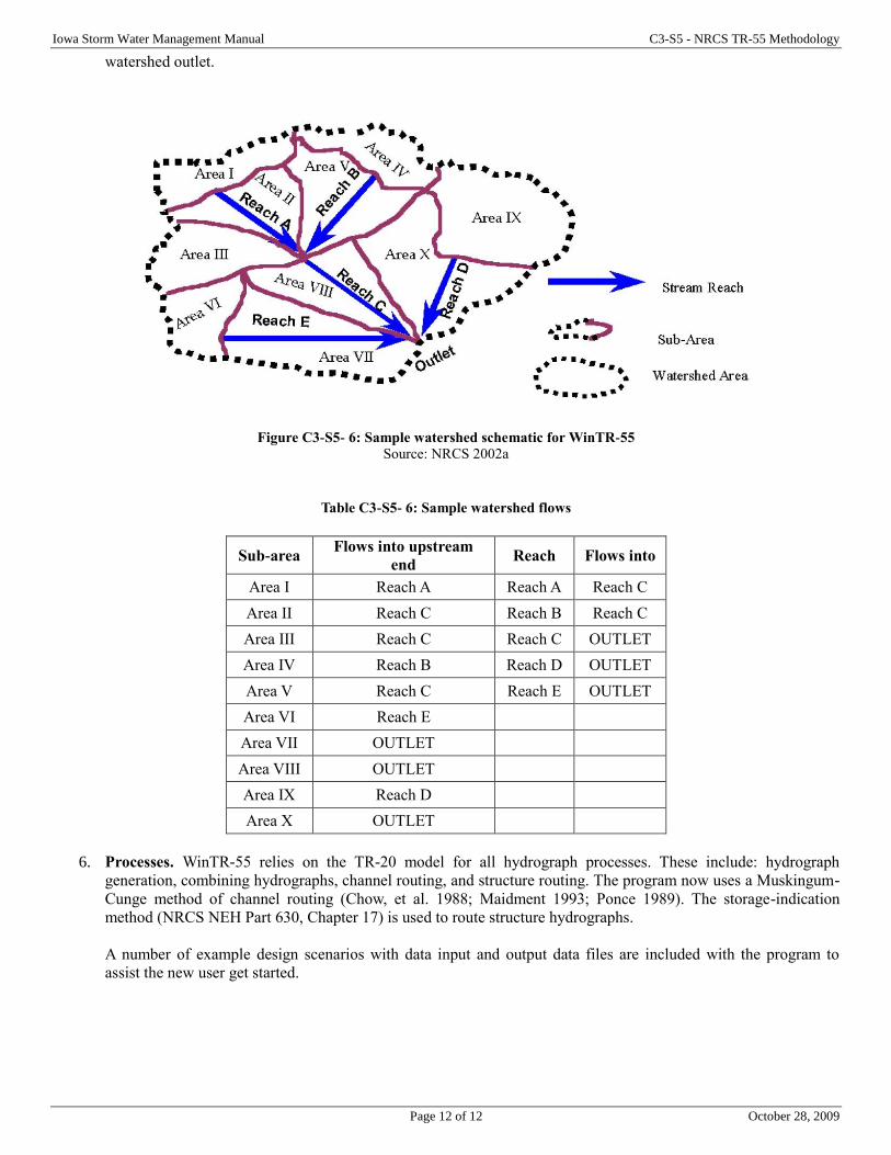
Iowa Storm Water Management Manual C3-S5 - NRCS TR-55 Methodology
Page 12 of 12 October 28, 2009
watershed outlet.
Figure C3-S5- 6: Sample watershed schematic for WinTR-55
Source: NRCS 2002a
Table C3-S5- 6: Sample watershed flows
Sub-area Flows into upstream
end Reach Flows into
Area I Reach A Reach A Reach C
Area II Reach C Reach B Reach C
Area III Reach C Reach C OUTLET
Area IV Reach B Reach D OUTLET
Area V Reach C Reach E OUTLET
Area VI Reach E
Area VII OUTLET
Area VIII OUTLET
Area IX Reach D
Area X OUTLET
6. Processes. WinTR-55 relies on the TR-20 model for all hydrograph processes. These include: hydrograph
generation, combining hydrographs, channel routing, and structure routing. The program now uses a Muskingum-
Cunge method of channel routing (Chow, et al. 1988; Maidment 1993; Ponce 1989). The storage-indication
method (NRCS NEH Part 630, Chapter 17) is used to route structure hydrographs.
A number of example design scenarios with data input and output data files are included with the program to
assist the new user get started.
Page 1 of 10 October 28, 2009
Chapter 3- Section 6 Small Storm Hydrology
A. Introduction
Water quality control designs are focused more on the annual runoff volume rather than peak storm events. Typically,
smaller storm events account for the majority of annual rainfall and runoff volumes. Three methods, based on varying
assumptions, and subsequently varying levels of complexity, are described in this section for determining the appropriate
water quality volume, water quality capture volume, and optimization of capture volume for detention basin systems. The
methods use storage volume as a surrogate for water quality, which is strictly a hydraulic issue and is the limitation of
these methods.
B. Water quality volume and peak flow
1. Water quality volume calculation. The water quality volume (WQv) is the treatment volume required to remove
a significant percentage of the stormwater pollution load, defined as an 80% removal of the average annual post-
development total suspended solids (TSS) load. This is achieved by intercepting and treating a portion of the
runoff from all storms and all the runoff from 90% of the storms that occur on average during the course of a year.
The water quality treatment volume is calculated by multiplying the 90th percentile annual rainfall event by the
volumetric runoff coefficient (Rv) and the site area. Rv is defined as:
Equation C3-S6- 1
𝑅𝑣 = 0.05 + 0.009(𝐼)
Where:
I = percent of impervious cover (%)
For the state of Iowa, the average 90% cumulative frequency annual rainfall event is 1.25 inches. The procedure
for determining the 90% cumulative frequency rainfall depth is described in Chapter 3, section 2.
Therefore, WQv is calculated using the following formula:
Equation C3-S6- 2
𝑊𝑄𝑣 = 𝑅𝑣 × 1.25𝑖𝑛𝑐ℎ𝑒𝑠 ×𝐴
12
Where:
WQv = water quality volume (ac-ft)
Rv = volumetric runoff coefficient
A = total drainage area (ac)
WQv can be expressed in inches simply as Qa =1.25Rv
Where:
Qa = runoff volume (in) for the water quality design rainfall event.
2. Water quality volume peak flow calculation. The peak rate of discharge is needed for the sizing of off-line
diversion structures and to design grass channels. Conventional NRCS methods underestimate the volume and
rate of runoff for rainfall events less than 2 inches. This discrepancy in estimating runoff and discharge rates can
lead to situations where a significant amount of runoff bypasses the filtering treatment practice due to an
inadequately-sized diversion structure, or leads to the design of undersized grass channels.
The following procedure can be used to estimate peak discharges for small storm events. It relies on the volume of
runoff computed using the small storm hydrology method (Pitt, 1994) and uses the NRCS WinTR-55 peak
discharge method.
Iowa Storm Water Management Manual C3-S6 - Small Storm Hydrology
Page 2 of 10 October 28, 2009
a. Step 1. Using the WQv, a corresponding curve number (CN) is computed from the following equation:
Equation C3-S6- 3
𝐶𝑁 =1000
[10 + 5𝑃 + 10𝑄𝑎] − 10(𝑄𝑎2 + 1.25𝑄𝑎𝑃)
12
Where:
P = rainfall, in inches (use 1.25 inches for the water quality storm in Iowa)
Qa = water quality runoff volume, in inches (1.25Rv)
Note: The above equation is derived from the NRCS runoff curve number method described in detail in NEH-
4, Hydrology (NRCS 1985) and NRCS TR-55 Chapter 2: Estimating Runoff. The CN can also be obtained
graphically using NRCS Figure D.10.1 or from WinTR-55.
b. Step 2. Once a CN is computed, the time of concentration (Tc) is computed (based on the methods in
identified in TR-55 and Chapter 3, section 3).
c. Step 3. Using the computed CN, Tc and drainage area (A), in acres, the peak discharge Qp is determined using
the procedure in WinTR-55. Note that the CN is computed manually outside the program and then entered
manually. The Tc computation menu in WinTR-55 can be used. The user will need to enter the water quality
design storm depth (1.25 inches) as well.
Note: When using WinTR-55 for this procedure, the user is cautioned to re-enter the original CN for the site when
going on to compute the peak rate, runoff volumes, and hydrographs for the larger 1-year through 100-year
recurrence intervals.
3. Example calculation of peak discharge for water quality storm. A 5-acre small commercial site has 1.2 acres
of flat roof, 3.4 acres of parking, and 0.4 acres of open space. The weighted volumetric runoff coefficient (Rv) is:
𝑅𝑣 = 0.05 + 0.009(𝐼) 𝐼 = 4.6 5.0⁄ = 0.92 (92%)
𝑅𝑣 = 0.05 + 0.009(92%)
𝑅𝑣 = 0.878 = 0.88
For the water quality rainfall depth of 1.25 inches, the runoff volume for this site is: 𝑄𝑎 = 𝑅𝑣 × 𝑃 = 0.88 ×1.25 𝑖𝑛𝑐ℎ𝑒𝑠 = 1.1 𝑤𝑎𝑡𝑒𝑟𝑠ℎ𝑒𝑑 𝑖𝑛𝑐ℎ𝑒𝑠.
WQv is:
𝑊𝑄𝑣 =[(1.25𝑖𝑛𝑐ℎ𝑒𝑠)(0.88)(5𝑎𝑐𝑟𝑒𝑠)]
12×
43,560𝑓𝑡2
𝑎𝑐𝑟𝑒𝑠= 19,995𝑓𝑡3
Using Qa = 1.1 watershed inches and P = 1.25 inches compute the CN for the WQ storm.
𝐶𝑁 =1000
[10 + (5)(1.25) + (10)(1.1𝑖𝑛𝑐ℎ𝑒𝑠)] − 10[(1.1𝑖𝑛𝑐ℎ𝑒𝑠)2 + 1.25(1.1)(1.25𝑖𝑛𝑐ℎ𝑒𝑠)]0.5= 98.6
(Use 98)
Using WinTR-55:
Manually enter the Tc = 10 minutes (0.17 hr) in the data entry menu
Enter the manually computed CN for the WQv rainfall (CN = 98)
Enter the watershed name and configuration when prompted
Enter the watershed area – 5 acres
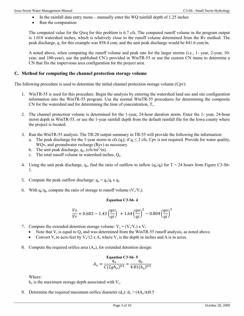
Iowa Storm Water Management Manual C3-S6 - Small Storm Hydrology
Page 3 of 10 October 28, 2009
In the rainfall data entry menu – manually enter the WQ rainfall depth of 1.25 inches
Run the computation
The computed value for the Qwq for this problem is 6.7 cfs. The computed runoff volume in the program output
is 1.018 watershed inches, which is relatively close to the runoff volume determined from the Rv method. The
peak discharge, q, for this example was 858.4 csm, and the unit peak discharge would be 841.6 csm/in.
A noted above, when computing the runoff volume and peak rate for the larger storms (i.e., 1- year, 2-year, 10-
year, and 100-year), use the published CN’s provided in WinTR-55 or use the custom CN menu to determine a
CN that fits the impervious area configuration for the project area.
C. Method for computing the channel protection storage volume
The following procedure is used to determine the initial channel protection storage volume (Cpv):
1. WinTR-55 is used for this procedure. Begin the analysis by entering the watershed land use and site configuration
information into the WinTR-55 program. Use the normal WinTR-55 procedures for determining the composite
CN for the watershed and for determining the time of concentration, Tc.
2. The channel protection volume is determined for the 1-year, 24-hour duration storm. Enter the 1- year, 24-hour
storm depth in WinTR-55, or use the 1-year rainfall depth from the default rainfall file for the Iowa county where
the project is located.
3. Run the WinTR-55 analysis. The TR-20 output summary in TR-55 will provide the following the information:
a. The peak discharge for the 1-year storm in cfs (qi); if qi ≤ 2 cfs, Cpv is not required. Provide for water quality,
WQv, and groundwater recharge (Rev) as necessary.
b. The unit peak discharge, qu, (cfs/mi2/in).
c. The total runoff volume in watershed inches, Qa.
4. Using the unit peak discharge, qu, find the ratio of outflow to inflow (qo/qi) for T = 24 hours from Figure C3-S6-
1.
5. Compute the peak outflow discharge: qo = qo/qi x qi.
6. With qo/qi, compute the ratio of storage to runoff volume (Vs/Vr).
Equation C3-S6- 4
𝑉𝑠
𝑉𝑟= 0.683 − 1.43 (
𝑞𝑜
𝑞𝑖) + 1.64 (
𝑞𝑜
𝑞𝑖)
2
− 0.804 (𝑞𝑜
𝑞𝑖)
3
7. Compute the extended detention storage volume: Vs = (Vs/Vr) x Vr
Note that Vr is equal to Qa and was determined from the WinTR-55 runoff analysis, as noted above.
Convert Vs to acre-feet by Vs/12 x A, where Vs is the depth in inches and A is in acres.
8. Compute the required orifice area (Ao), for extended detention design:
Equation C3-S6- 5
𝐴𝑜 =𝑞𝑜
𝐶(2𝑔ℎ𝑜)0.5=
𝑞𝑜
4.81(ℎ𝑜)0.5
Where:
ho is the maximum storage depth associated with Vs.
9. Determine the required maximum orifice diameter (do): do = (4Ao/π)0.5
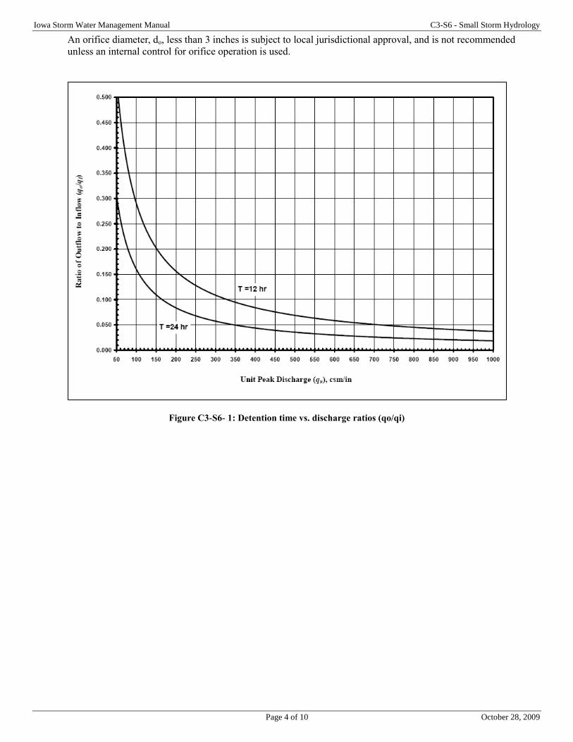
Iowa Storm Water Management Manual C3-S6 - Small Storm Hydrology
Page 4 of 10 October 28, 2009
An orifice diameter, do, less than 3 inches is subject to local jurisdictional approval, and is not recommended
unless an internal control for orifice operation is used.
Figure C3-S6- 1: Detention time vs. discharge ratios (qo/qi)
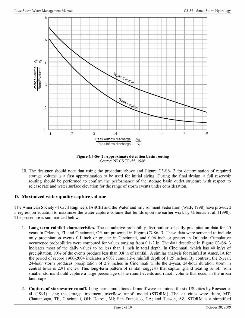
Iowa Storm Water Management Manual C3-S6 - Small Storm Hydrology
Page 5 of 10 October 28, 2009
Figure C3-S6- 2: Approximate detention basin routing
Source: NRCS TR-55, 1986
10. The designer should note that using the procedure above and Figure C3-S6- 2 for determination of required
storage volume is a first approximation to be used for initial sizing. During the final design, a full reservoir
routing should be performed to confirm the performance of the storage basin outlet structure with respect to
release rate and water surface elevation for the range of storm events under consideration.
D. Maximized water quality capture volume
The American Society of Civil Engineers (ASCE) and the Water and Environment Federation (WEF, 1998) have provided
a regression equation to maximize the water capture volume that builds upon the earlier work by Urbonas et al. (1990).
The procedure is summarized below:
1. Long-term rainfall characteristics. The cumulative probability distributions of daily precipitation data for 40
years in Orlando, FL and Cincinnati, OH are presented in Figure C3-S6- 3. These data were screened to include
only precipitation events 0.1 inch or greater in Cincinnati, and 0.06 inch or greater in Orlando. Cumulative
occurrence probabilities were computed for values ranging from 0.1-2 in. The data described in Figure C3-S6- 3
indicates most of the daily values to be less than 1 inch in total depth. In Cincinnati, which has 40 in/yr of
precipitation, 90% of the events produce less than 0.8 in of rainfall. A similar analysis for rainfall at Ames, IA for
the period of record 1960-2004 indicates a 90% cumulative rainfall depth of 1.25 inches. By contrast, the 2-year,
24-hour storm produces precipitation of 2.9 inches in Cincinnati while the 2-year, 24-hour duration storm in
central Iowa is 2.91 inches. This long-term pattern of rainfall suggests that capturing and treating runoff from
smaller storms should capture a large percentage of the runoff events and runoff volume that occur in the urban
landscape.
2. Capture of stormwater runoff. Long-term simulations of runoff were examined for six US cities by Roesner et
al. (1991) using the storage, treatment, overflow, runoff model (STORM). The six cities were Butte, MT;
Chattanooga, TE; Cincinnati, OH; Detroit, MI; San Francisco, CA; and Tucson, AZ. STORM is a simplified
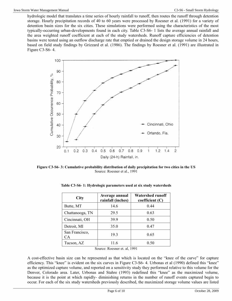
Iowa Storm Water Management Manual C3-S6 - Small Storm Hydrology
Page 6 of 10 October 28, 2009
hydrologic model that translates a time series of hourly rainfall to runoff, then routes the runoff through detention
storage. Hourly precipitation records of 40 to 60 years were processed by Roesner et al. (1991) for a variety of
detention basin sizes for the six cities. These simulations were performed using the characteristics of the most
typically-occurring urban-developments found in each city. Table C3-S6- 1 lists the average annual rainfall and
the area weighted runoff coefficient at each of the study watersheds. Runoff capture efficiencies of detention
basins were tested using an outflow discharge rate that emptied or drained the design storage volume in 24 hours,
based on field study findings by Grizzard et al. (1986). The findings by Roesner et al. (1991) are illustrated in
Figure C3-S6- 4.
Figure C3-S6- 3: Cumulative probability distribution of daily precipitation for two cities in the US
Source: Roesner et al., 1991
Table C3-S6- 1: Hydrologic parameters used at six study watersheds
City Average annual
rainfall (inches)
Watershed runoff
coefficient (C)
Butte, MT 14.6 0.44
Chattanooga, TN 29.5 0.63
Cincinnati, OH 39.9 0.50
Detroit, MI 35.0 0.47
San Francisco,
CA 19.3 0.65
Tucson, AZ 11.6 0.50
Source: Roesner et. al, 1991
A cost-effective basin size can be represented as that which is located on the “knee of the curve” for capture
efficiency. This “knee” is evident on the six curves in Figure C3-S6- 4. Urbonas et al (1990) defined this “knee”
as the optimized capture volume, and reported on a sensitivity study they performed relative to this volume for the
Denver, Colorado area. Later, Urbonas and Stahre (1993) redefined this “knee” as the maximized volume,
because it is the point at which rapidly- diminishing returns in the number of runoff events captured begin to
occur. For each of the six study watersheds previously described, the maximized storage volume values are listed
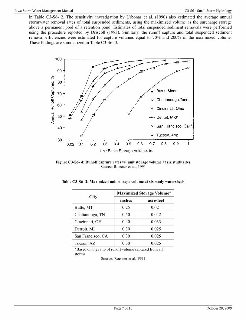
Iowa Storm Water Management Manual C3-S6 - Small Storm Hydrology
Page 7 of 10 October 28, 2009
in Table C3-S6- 2. The sensitivity investigation by Urbonas et al. (1990) also estimated the average annual
stormwater removal rates of total suspended sediments, using the maximized volume as the surcharge storage
above a permanent pool of a retention pond. Estimates of total suspended sediment removals were performed
using the procedure reported by Driscoll (1983). Similarly, the runoff capture and total suspended sediment
removal efficiencies were estimated for capture volumes equal to 70% and 200% of the maximized volume.
These findings are summarized in Table C3-S6- 3.
Figure C3-S6- 4: Runoff capture rates vs. unit storage volume at six study sites
Source: Roesner et al., 1991
Table C3-S6- 2: Maximized unit storage volume at six study watersheds
City Maximized Storage Volume*
inches acre-feet
Butte, MT 0.25 0.021
Chattanooga, TN 0.50 0.042
Cincinnati, OH 0.40 0.033
Detroit, MI 0.30 0.025
San Francisco, CA 0.30 0.025
Tucson, AZ 0.30 0.025
*Based on the ratio of runoff volume captured from all
storms Source: Roesner et al, 1991
Iowa Storm Water Management Manual C3-S6 - Small Storm Hydrology
Page 8 of 10 October 28, 2009
Table C3-S6- 3: Sensitivity of the BMP capture volume in Denver, CO
Capture volume to
maximized volume
ratio
Annual runoff
volume captured
(%)
No. storms
completely captured
Average annual
TSS removed (%)
0.7 75 27 86
0.7 85 30 88
2.0 94 33 90
Source: Urbonas et al, 1990
As can be seen from Figure C3-S6- 4 and Table C3-S6- 2 and Table C3-S6- 3, most runoff-producing events occur
as a result of the predominant population of smaller storms, namely, less than 0.5-1.25 inches of precipitation. To
be effective, stormwater quality management should be designed based on these smaller events. As a result,
detention facilities, wetland basins, infiltration facilities, media filters, grass swales, and other treatment BMPs
should be sized to accommodate runoff volumes and flows from such storm events to maximize pollution control
benefits in a cost-effective manner.
E. Estimating a maximized water quality capture volume
When local resources permit, the stormwater quality capture volume may best be found using continuous
hydrologic simulation and local long-term hourly (or 15-minute time increment) precipitation records. However, it
is possible to obtain a first-order estimate of the needed capture volume using simplified procedures that target the
most typically-occurring population of runoff events. Figure C3-S6- 5 contains a map of the contiguous 48 states
of the US with the mean annual runoff-producing rainfall depths superimposed (Driscoll et al., 1989). The mean
depths are based on a 6-hour inter-event time to define a new storm event, and a minimum depth of 0.10 inches of
precipitation for a storm to produce incipient runoff. Guo and Urbonas (1995) found simple regression equations
to relate the mean precipitation depths in Figure C3-S6- 5 to maximized water quality runoff capture volumes (the
“knee” of the cumulative probability curve). The analytical procedure was based on a simple transformation of
each storm's volume of precipitation to a runoff volume using a runoff coefficient, C. A third-order regression
equation, Equation C3-S6- 1 (Urbonas et al., 1990) was derived using data from the 1983 NURP studies of more
than 60 urban watersheds over a two- year period (EPA, 1983). Since the data was collected nationally over a two-
year period, Equation C3-S6- 1 will have broad applicability in the US, for smaller storm events.
Equation C3-S6- 6
𝐶 = 0.858𝑖3 − 0.78𝑖2 − 0.774𝑖 + 0.04
Where:
C = runoff coefficient
i = watershed imperviousness ratio (percent total imperviousness divided by 100)
Equation C3-S6- 6 relates mean precipitation depth taken from Figure C3-S6- 5 to the maximized detention
volume. The coefficients listed in Table C3-S6- 4 are based on an analysis of long-term data from seven
precipitation- gauging sites located in different meteorological regions of the US. The correlation of determination
coefficient, R2, has a range of 0.80-0.97.
Equation C3-S6- 7
𝑃0 = (𝑎)(𝐶)(𝑃6)
Where:
P0 = maximized detention volume in watershed-inches (determined using either the event or volume capture ratio “a”
from Table C3-S6- 4)
a = regression constant from least-squares analysis
C = watershed runoff coefficient
Iowa Storm Water Management Manual C3-S6 - Small Storm Hydrology
Page 9 of 10 October 28, 2009
P6 = mean storm precipitation volume (watershed inches) (Figure C3-S6- 5 or local data)
The mean precipitation value, P6, can be obtained from Figure C3-S6- 5 or referenced from local rainfall data.
The maximized detention volume, P0, can determined using either the event capture ratio or the volume capture ratio as its
basis. Table C3-S6- 4 lists the maximized detention volume/mean precipitation ratios based on either the ratio of the total
number of storm runoff events captured, or the fraction of the total stormwater runoff volume from a catchment. These
can be used to estimate the annual average maximized detention volume at any given site. All that is needed is the
watershed’s “C” and its mean annual precipitation, P6. The actual size of the runoff event to target for water quality
enhancement should be based on the evaluation of local hydrology and water quality needs. However, examination of
Table C3-S6- 4 indicates that the use of larger detention volumes does not significantly improve the average annual
removal of total suspended sediments or other settleable constituents. It is likely that an extended detention volume equal
to a volume between the runoff from a mean precipitation event taken from Figure C3-S6- 5 and the maximized event
obtained using Equation C3-S6- 7 will provide the optimumly-sized and most cost-effective BMP facility. A BMP sized to
capture such a volume will also capture the leading edge (first flush) of the runoff hydrograph resulting from larger
storms. Runoff volumes that exceed the design detention volume either bypass the facility or receive less-efficient
treatment than do the smaller volume storms, and have only a minimal net effect on the detention basin’s performance. If,
however, the design volume is larger and has an outlet to drain it in the same amount of time as the smaller basin, the
smallest runoff events will be detained only for a brief interval by the larger outlet. Analysis of long-term precipitation
records in the US shows that small events always seem to have the greatest preponderance. Therefore, over-sizing the
detention can cause the most frequent runoff events to receive less treatment than provided by properly-designed small
basins.
Table C3-S6- 4: Values of coefficient “a” in Equation C3-S6- 7 for finding the maximized detention storage volume*
Drain time of capture
volume
12-hr 24-hr 48-hr
Event capture ratio a = 1.109 1.299 1.545
r2 = 0.97 0.91 0.85
Volume capture ratio a = 1.312 1.582 1.963
r2 = 0.80 0.93 0.85
*Approximately 85th
percentile runoff event (range 82-88%)
Source: Guo and Urbonas, 1995
F. Design example
Water quality capture volume estimate
A project site in the western suburbs of Des Moines, IA has a 280-acre watershed. At full build-out, the project is expected
to have about 36% of its area covered by impervious surface. A regional detention basin is one of the alternatives being
considered for water quality enhancement. Determine the maximized storage volume. The detention basin needs to be
sized and designed to drain its water quality capture volume in 24 hours.
1. Determine the C value for the project watershed, using Equation C3-S6- 6 (i = 0.36):
𝐶 = 0.858𝑖3 − 0.78𝑖2 − 0.774𝑖 + 0.040.858(0.36)3 − 0.78(0.36)2 − 0.774(0.36) + 0.04 = 0.26
2. Determine the mean precipitation depth, P6, for the Des Moines area from Figure C3-S6- 5:
P6 = 0.57 inches
3. From Table C3-S6- 4, find the coefficient a = 1.299 for the 24-hour drain time. The maximized detention volume
is calculated as follows from Equation C3-S6- 7:
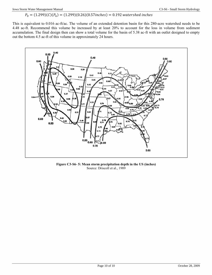
Iowa Storm Water Management Manual C3-S6 - Small Storm Hydrology
Page 10 of 10 October 28, 2009
𝑃0 = (1.299)(𝐶)(𝑃6) = (1.299)(0.26)(0.57𝑖𝑛𝑐ℎ𝑒𝑠) = 0.192 𝑤𝑎𝑡𝑒𝑟𝑠ℎ𝑒𝑑 𝑖𝑛𝑐ℎ𝑒𝑠
This is equivalent to 0.016 ac-ft/ac. The volume of an extended detention basin for this 280-acre watershed needs to be
4.48 ac-ft. Recommend this volume be increased by at least 20% to account for the loss in volume from sediment
accumulation. The final design then can show a total volume for the basin of 5.38 ac-ft with an outlet designed to empty
out the bottom 4.5 ac-ft of this volume in approximately 24 hours.
Figure C3-S6- 5: Mean storm precipitation depth in the US (inches)
Source: Driscoll et al., 1989

Page 1 of 19 October 28, 2009
Chapter 3- Section 7 Runoff Hydrograph Determination
A. Introduction
The runoff discharge hydrograph is a graph of discharge rate versus time, where the discharge is in units of volume/time
(i.e., ft3/sec, acre-ft/day). The runoff hydrograph can also be expressed as might be defined for a stage-discharge
relationship for a stream channel of floodway (i.e., the discharge rating curve for a channel cross section). The shape of
the storm hydrograph is related to the rainfall hyetograph (intensity vs. time) and the combined effects of the storage in
the watershed or channel. The watershed and channel storage effects smooth out much of the variation evident in the
storm hyetograph. The runoff hydrograph increases in magnitude shortly after the start of the rainfall event and reaches a
peak after the maximum rainfall intensity has occurred.
For the design of storm sewers and culverts, the required pipe or culvert diameter is typically based on based on
conveyance capacity for the peak discharge, and a hydrograph is not typically used for the analysis. As a watershed
becomes more urbanized, the impact of more impervious area, decreased potential for infiltration, and loss of natural
depression storage will change the response to rainfall and thus the shape (peak and time base) of the resulting runoff
hydrograph. When routing runoff through a stream reach or where detention storage will be used, an inflow (upstream)
hydrograph must be determined.
B. Unit hydrographs
The unit hydrograph is defined as the hydrograph of direct runoff that results from 1 inch of excess rainfall generated
uniformly over the watershed at a constant rate during a specified time. A T-hour (or T-minute) hydrograph is the
hydrograph resulting from a storm with a continuous rainfall excess of 1 inch over the duration to T-hours (or T-minutes).
Another common unit hydrograph used in urban hydrology is the dimensionless unit hydrograph. The ordinates of the
dimensionless unit hydrograph are expressed as ratios of the peak discharge (q/qp) and the time axis (abscissa) is given as
ratios of the time to the time to peak (t/tp), where qp is the discharge rate at the time to peak, tp.
In hydrograph analysis, the storm hyetograph (rainfall input function) is converted to the direct runoff hydrograph (output)
in common design practice using a unit hydrograph (transfer function). In an event-based model such as the NRCS
method (WinTR-55 and WinTR-20), the rainfall hyetograph for the design rainfall event is based on the CN method and
the application of the NRCS 24-hour rainfall distribution (Chapter 3, section 2). The NRCS dimensionless unit
hydrograph (1985) is frequently used in practice, is well-documented, and is recommended for design of BMPs included
in this manual. In development of the method, a large number of actual watersheds were evaluated and then made
dimensionless by dividing all discharge ordinates by the peak discharge and the time values by the time to peak. An
average of these dimensionless unit hydrographs (UH) was computed. The time-base of the dimensionless UH is
approximately five times the time to peak, and approximately ⅜ of the total volume occurred before the time to peak. The
inflection point on the recession limb occurs at about 1.7 times the time to peak, and the hydrograph has a curvilinear
shape. The curvilinear hydrograph can be approximated by a triangular UH with similar characteristics. The average
dimensionless curvilinear UH and triangular UH are illustrated in Figure C3-S7- 1. While the time base of the triangular
UH is only ⅜ of the time to peak (5 for the dimensionless UH), the area under the rising limb of both UH’s is the same
(37.5%). The discharge ratios for the NRCS dimensionless UH are given in Table C3-S7- 1.
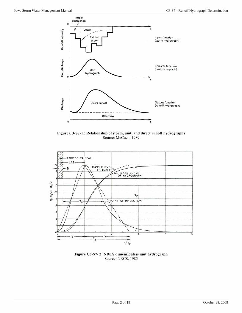
Iowa Storm Water Management Manual C3-S7 - Runoff Hydrograph Determination
Page 2 of 19 October 28, 2009
Figure C3-S7- 1: Relationship of storm, unit, and direct runoff hydrographs
Source: McCuen, 1989
Figure C3-S7- 2: NRCS dimensionless unit hydrograph
Source: NRCS, 1985
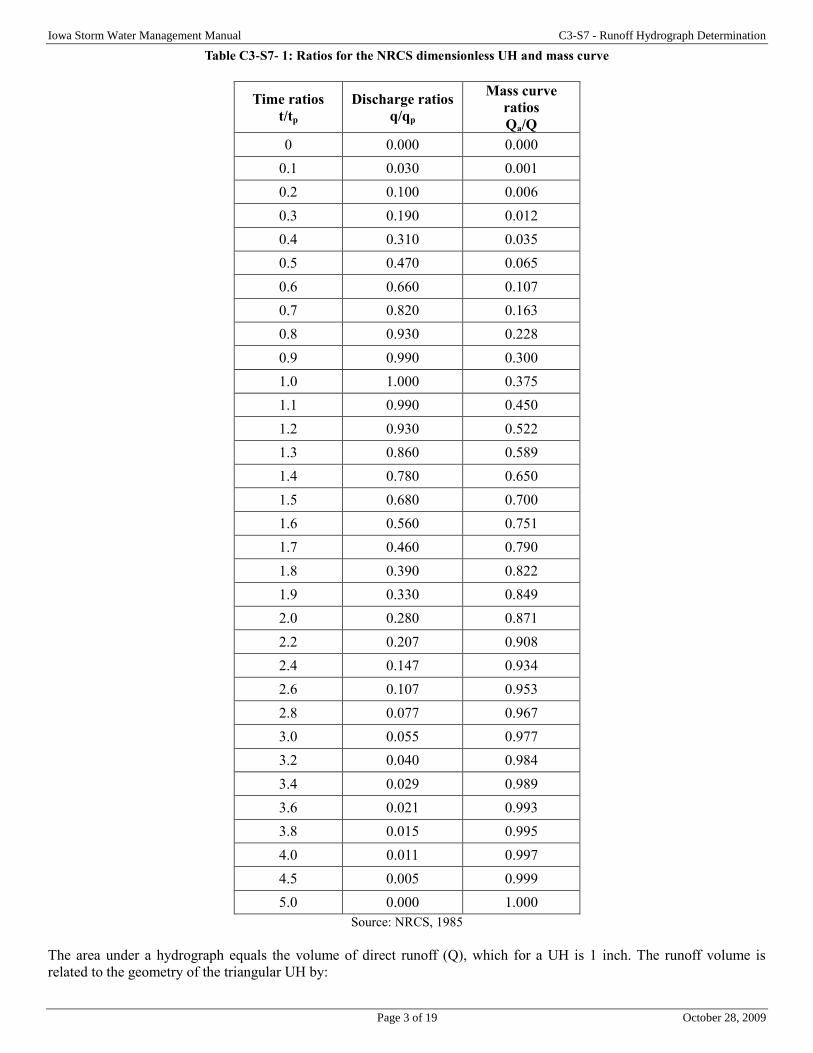
Iowa Storm Water Management Manual C3-S7 - Runoff Hydrograph Determination
Page 3 of 19 October 28, 2009
Table C3-S7- 1: Ratios for the NRCS dimensionless UH and mass curve
Time ratios
t/tp
Discharge ratios
q/qp
Mass curve
ratios
Qa/Q
0 0.000 0.000
0.1 0.030 0.001
0.2 0.100 0.006
0.3 0.190 0.012
0.4 0.310 0.035
0.5 0.470 0.065
0.6 0.660 0.107
0.7 0.820 0.163
0.8 0.930 0.228
0.9 0.990 0.300
1.0 1.000 0.375
1.1 0.990 0.450
1.2 0.930 0.522
1.3 0.860 0.589
1.4 0.780 0.650
1.5 0.680 0.700
1.6 0.560 0.751
1.7 0.460 0.790
1.8 0.390 0.822
1.9 0.330 0.849
2.0 0.280 0.871
2.2 0.207 0.908
2.4 0.147 0.934
2.6 0.107 0.953
2.8 0.077 0.967
3.0 0.055 0.977
3.2 0.040 0.984
3.4 0.029 0.989
3.6 0.021 0.993
3.8 0.015 0.995
4.0 0.011 0.997
4.5 0.005 0.999
5.0 0.000 1.000
Source: NRCS, 1985
The area under a hydrograph equals the volume of direct runoff (Q), which for a UH is 1 inch. The runoff volume is
related to the geometry of the triangular UH by:
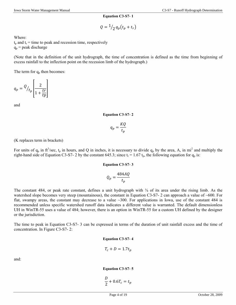
Iowa Storm Water Management Manual C3-S7 - Runoff Hydrograph Determination
Page 4 of 19 October 28, 2009
Equation C3-S7- 1
𝑄 = 12⁄ 𝑞𝑝(𝑡𝑝 + 𝑡𝑟)
Where:
tp and tr = time to peak and recession time, respectively
qp = peak discharge
(Note that in the definition of the unit hydrograph, the time of concentration is defined as the time from beginning of
excess rainfall to the inflection point on the recession limb of the hydrograph.)
The term for qp then becomes:
𝑞𝑝 =𝑄
𝑡𝑝⁄ [
2
1 +𝑡𝑟𝑡𝑝
]
and
Equation C3-S7- 2
𝑞𝑝 =𝐾𝑄
𝑡𝑝
(K replaces term in brackets)
For units of qp in ft3/sec, tp in hours, and Q in inches, it is necessary to divide qp by the area, A, in mi
2 and multiply the
right-hand side of Equation C3-S7- 2 by the constant 645.3; since tr = 1.67 tp, the following equation for qp is:
Equation C3-S7- 3
𝑄𝑝 =484𝐴𝑄
𝑡𝑝
The constant 484, or peak rate constant, defines a unit hydrograph with ⅜ of its area under the rising limb. As the
watershed slope becomes very steep (mountainous), the constant in Equation C3-S7- 2 can approach a value of ~600. For
flat, swampy areas, the constant may decrease to a value ~300. For applications in Iowa, use of the constant 484 is
recommended unless specific watershed runoff data indicates a different value is warranted. The default dimensionless
UH in WinTR-55 uses a value of 484; however, there is an option in WinTR-55 for a custom UH defined by the designer
or the jurisdiction.
The time to peak in Equation C3-S7- 3 can be expressed in terms of the duration of unit rainfall excess and the time of
concentration. In Figure C3-S7- 2:
Equation C3-S7- 4
𝑇𝑐 + 𝐷 = 1.7𝑡𝑝
and:
Equation C3-S7- 5
𝐷
2+ 0.6𝑇𝑐 = 𝑡𝑝
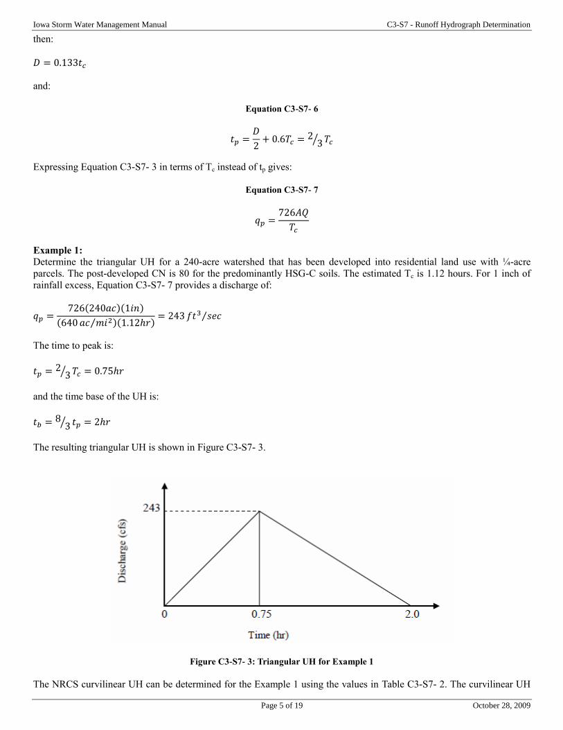
Iowa Storm Water Management Manual C3-S7 - Runoff Hydrograph Determination
Page 5 of 19 October 28, 2009
then:
𝐷 = 0.133𝑡𝑐
and:
Equation C3-S7- 6
𝑡𝑝 =𝐷
2+ 0.6𝑇𝑐 = 2
3⁄ 𝑇𝑐
Expressing Equation C3-S7- 3 in terms of Tc instead of tp gives:
Equation C3-S7- 7
𝑞𝑝 =726𝐴𝑄
𝑇𝑐
Example 1:
Determine the triangular UH for a 240-acre watershed that has been developed into residential land use with ¼-acre
parcels. The post-developed CN is 80 for the predominantly HSG-C soils. The estimated Tc is 1.12 hours. For 1 inch of
rainfall excess, Equation C3-S7- 7 provides a discharge of:
𝑞𝑝 =726(240𝑎𝑐)(1𝑖𝑛)
(640 𝑎𝑐 𝑚𝑖2⁄ )(1.12ℎ𝑟)= 243 𝑓𝑡3 𝑠𝑒𝑐⁄
The time to peak is:
𝑡𝑝 = 23⁄ 𝑇𝑐 = 0.75ℎ𝑟
and the time base of the UH is:
𝑡𝑏 = 83⁄ 𝑡𝑝 = 2ℎ𝑟
The resulting triangular UH is shown in Figure C3-S7- 3.
Figure C3-S7- 3: Triangular UH for Example 1
The NRCS curvilinear UH can be determined for the Example 1 using the values in Table C3-S7- 2. The curvilinear UH
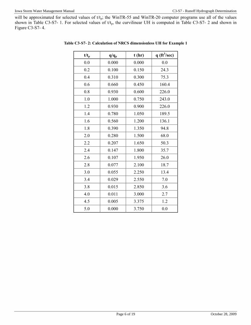
Iowa Storm Water Management Manual C3-S7 - Runoff Hydrograph Determination
Page 6 of 19 October 28, 2009
will be approximated for selected values of t/tp; the WinTR-55 and WinTR-20 computer programs use all of the values
shown in Table C3-S7- 1. For selected values of t/tp, the curvilinear UH is computed in Table C3-S7- 2 and shown in
Figure C3-S7- 4.
Table C3-S7- 2: Calculation of NRCS dimensionless UH for Example 1
t/tp q/qp t (hr) q (ft3/sec)
0.0 0.000 0.000 0.0
0.2 0.100 0.150 24.3
0.4 0.310 0.300 75.3
0.6 0.660 0.450 160.4
0.8 0.930 0.600 226.0
1.0 1.000 0.750 243.0
1.2 0.930 0.900 226.0
1.4 0.780 1.050 189.5
1.6 0.560 1.200 136.1
1.8 0.390 1.350 94.8
2.0 0.280 1.500 68.0
2.2 0.207 1.650 50.3
2.4 0.147 1.800 35.7
2.6 0.107 1.950 26.0
2.8 0.077 2.100 18.7
3.0 0.055 2.250 13.4
3.4 0.029 2.550 7.0
3.8 0.015 2.850 3.6
4.0 0.011 3.000 2.7
4.5 0.005 3.375 1.2
5.0 0.000 3.750 0.0
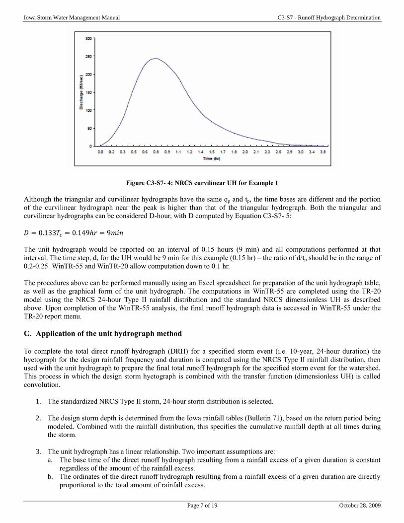
Iowa Storm Water Management Manual C3-S7 - Runoff Hydrograph Determination
Page 7 of 19 October 28, 2009
Figure C3-S7- 4: NRCS curvilinear UH for Example 1
Although the triangular and curvilinear hydrographs have the same qp and tp, the time bases are different and the portion
of the curvilinear hydrograph near the peak is higher than that of the triangular hydrograph. Both the triangular and
curvilinear hydrographs can be considered D-hour, with D computed by Equation C3-S7- 5:
𝐷 = 0.133𝑇𝑐 = 0.149ℎ𝑟 = 9𝑚𝑖𝑛
The unit hydrograph would be reported on an interval of 0.15 hours (9 min) and all computations performed at that
interval. The time step, d, for the UH would be 9 min for this example (0.15 hr) – the ratio of d/tp should be in the range of
0.2-0.25. WinTR-55 and WinTR-20 allow computation down to 0.1 hr.
The procedures above can be performed manually using an Excel spreadsheet for preparation of the unit hydrograph table,
as well as the graphical form of the unit hydrograph. The computations in WinTR-55 are completed using the TR-20
model using the NRCS 24-hour Type II rainfall distribution and the standard NRCS dimensionless UH as described
above. Upon completion of the WinTR-55 analysis, the final runoff hydrograph data is accessed in WinTR-55 under the
TR-20 report menu.
C. Application of the unit hydrograph method
To complete the total direct runoff hydrograph (DRH) for a specified storm event (i.e. 10-year, 24-hour duration) the
hyetograph for the design rainfall frequency and duration is computed using the NRCS Type II rainfall distribution, then
used with the unit hydrograph to prepare the final total runoff hydrograph for the specified storm event for the watershed.
This process in which the design storm hyetograph is combined with the transfer function (dimensionless UH) is called
convolution.
1. The standardized NRCS Type II storm, 24-hour storm distribution is selected.
2. The design storm depth is determined from the Iowa rainfall tables (Bulletin 71), based on the return period being
modeled. Combined with the rainfall distribution, this specifies the cumulative rainfall depth at all times during
the storm.
3. The unit hydrograph has a linear relationship. Two important assumptions are:
a. The base time of the direct runoff hydrograph resulting from a rainfall excess of a given duration is constant
regardless of the amount of the rainfall excess.
b. The ordinates of the direct runoff hydrograph resulting from a rainfall excess of a given duration are directly
proportional to the total amount of rainfall excess.
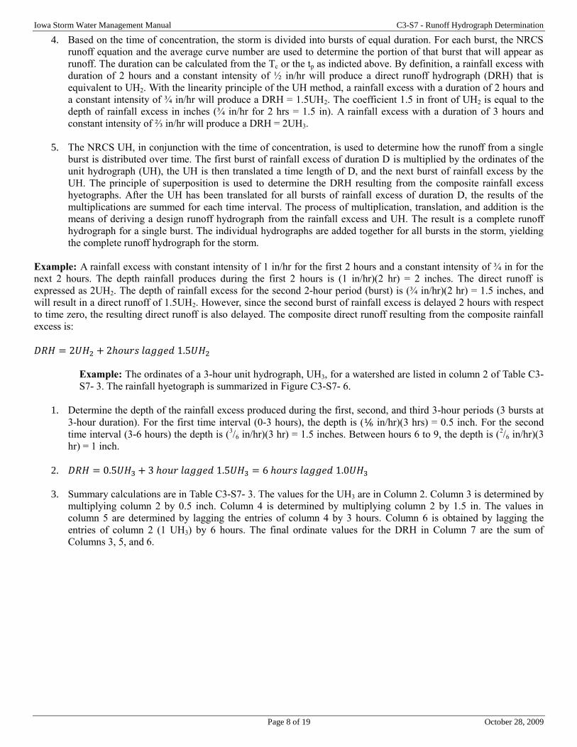
Iowa Storm Water Management Manual C3-S7 - Runoff Hydrograph Determination
Page 8 of 19 October 28, 2009
4. Based on the time of concentration, the storm is divided into bursts of equal duration. For each burst, the NRCS
runoff equation and the average curve number are used to determine the portion of that burst that will appear as
runoff. The duration can be calculated from the Tc or the tp as indicted above. By definition, a rainfall excess with
duration of 2 hours and a constant intensity of ½ in/hr will produce a direct runoff hydrograph (DRH) that is
equivalent to UH2. With the linearity principle of the UH method, a rainfall excess with a duration of 2 hours and
a constant intensity of ¾ in/hr will produce a DRH = 1.5UH2. The coefficient 1.5 in front of UH2 is equal to the
depth of rainfall excess in inches (¾ in/hr for 2 hrs = 1.5 in). A rainfall excess with a duration of 3 hours and
constant intensity of ⅔ in/hr will produce a DRH = 2UH3.
5. The NRCS UH, in conjunction with the time of concentration, is used to determine how the runoff from a single
burst is distributed over time. The first burst of rainfall excess of duration D is multiplied by the ordinates of the
unit hydrograph (UH), the UH is then translated a time length of D, and the next burst of rainfall excess by the
UH. The principle of superposition is used to determine the DRH resulting from the composite rainfall excess
hyetographs. After the UH has been translated for all bursts of rainfall excess of duration D, the results of the
multiplications are summed for each time interval. The process of multiplication, translation, and addition is the
means of deriving a design runoff hydrograph from the rainfall excess and UH. The result is a complete runoff
hydrograph for a single burst. The individual hydrographs are added together for all bursts in the storm, yielding
the complete runoff hydrograph for the storm.
Example: A rainfall excess with constant intensity of 1 in/hr for the first 2 hours and a constant intensity of ¾ in for the
next 2 hours. The depth rainfall produces during the first 2 hours is (1 in/hr)(2 hr) = 2 inches. The direct runoff is
expressed as 2UH2. The depth of rainfall excess for the second 2-hour period (burst) is (¾ in/hr)(2 hr) = 1.5 inches, and
will result in a direct runoff of 1.5UH2. However, since the second burst of rainfall excess is delayed 2 hours with respect
to time zero, the resulting direct runoff is also delayed. The composite direct runoff resulting from the composite rainfall
excess is:
𝐷𝑅𝐻 = 2𝑈𝐻2 + 2ℎ𝑜𝑢𝑟𝑠 𝑙𝑎𝑔𝑔𝑒𝑑 1.5𝑈𝐻2
Example: The ordinates of a 3-hour unit hydrograph, UH3, for a watershed are listed in column 2 of Table C3-
S7- 3. The rainfall hyetograph is summarized in Figure C3-S7- 6.
1. Determine the depth of the rainfall excess produced during the first, second, and third 3-hour periods (3 bursts at
3-hour duration). For the first time interval (0-3 hours), the depth is (⅙ in/hr)(3 hrs) = 0.5 inch. For the second
time interval (3-6 hours) the depth is (3/6 in/hr)(3 hr) = 1.5 inches. Between hours 6 to 9, the depth is (
2/6 in/hr)(3
hr) = 1 inch.
2. 𝐷𝑅𝐻 = 0.5𝑈𝐻3 + 3 ℎ𝑜𝑢𝑟 𝑙𝑎𝑔𝑔𝑒𝑑 1.5𝑈𝐻3 = 6 ℎ𝑜𝑢𝑟𝑠 𝑙𝑎𝑔𝑔𝑒𝑑 1.0𝑈𝐻3
3. Summary calculations are in Table C3-S7- 3. The values for the UH3 are in Column 2. Column 3 is determined by
multiplying column 2 by 0.5 inch. Column 4 is determined by multiplying column 2 by 1.5 in. The values in
column 5 are determined by lagging the entries of column 4 by 3 hours. Column 6 is obtained by lagging the
entries of column 2 (1 UH3) by 6 hours. The final ordinate values for the DRH in Column 7 are the sum of
Columns 3, 5, and 6.
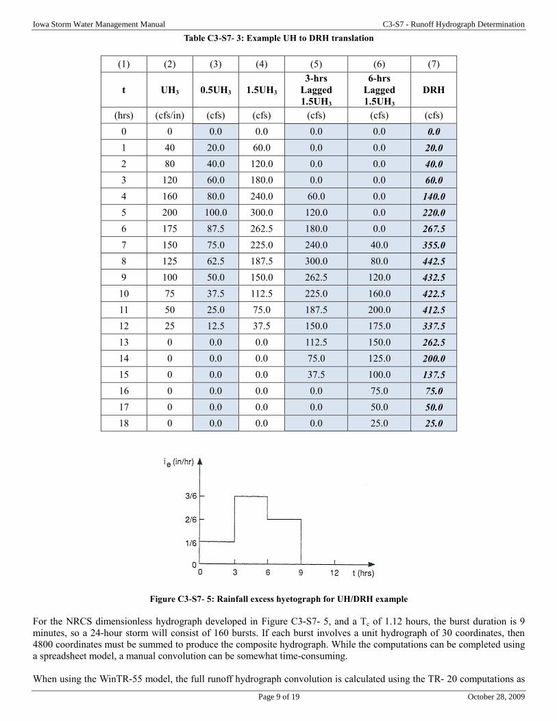
Iowa Storm Water Management Manual C3-S7 - Runoff Hydrograph Determination
Page 9 of 19 October 28, 2009
Table C3-S7- 3: Example UH to DRH translation
(1) (2) (3) (4) (5) (6) (7)
t UH3 0.5UH3 1.5UH3
3-hrs
Lagged
1.5UH3
6-hrs
Lagged
1.5UH3
DRH
(hrs) (cfs/in) (cfs) (cfs) (cfs) (cfs) (cfs)
0 0 0.0 0.0 0.0 0.0 0.0
1 40 20.0 60.0 0.0 0.0 20.0
2 80 40.0 120.0 0.0 0.0 40.0
3 120 60.0 180.0 0.0 0.0 60.0
4 160 80.0 240.0 60.0 0.0 140.0
5 200 100.0 300.0 120.0 0.0 220.0
6 175 87.5 262.5 180.0 0.0 267.5
7 150 75.0 225.0 240.0 40.0 355.0
8 125 62.5 187.5 300.0 80.0 442.5
9 100 50.0 150.0 262.5 120.0 432.5
10 75 37.5 112.5 225.0 160.0 422.5
11 50 25.0 75.0 187.5 200.0 412.5
12 25 12.5 37.5 150.0 175.0 337.5
13 0 0.0 0.0 112.5 150.0 262.5
14 0 0.0 0.0 75.0 125.0 200.0
15 0 0.0 0.0 37.5 100.0 137.5
16 0 0.0 0.0 0.0 75.0 75.0
17 0 0.0 0.0 0.0 50.0 50.0
18 0 0.0 0.0 0.0 25.0 25.0
Figure C3-S7- 5: Rainfall excess hyetograph for UH/DRH example
For the NRCS dimensionless hydrograph developed in Figure C3-S7- 5, and a Tc of 1.12 hours, the burst duration is 9
minutes, so a 24-hour storm will consist of 160 bursts. If each burst involves a unit hydrograph of 30 coordinates, then
4800 coordinates must be summed to produce the composite hydrograph. While the computations can be completed using
a spreadsheet model, a manual convolution can be somewhat time-consuming.
When using the WinTR-55 model, the full runoff hydrograph convolution is calculated using the TR- 20 computations as
Iowa Storm Water Management Manual C3-S7 - Runoff Hydrograph Determination
Page 10 of 19 October 28, 2009
described above, and the hyetograph for each storm frequency is automatically generated using the standard NRCS 24-
hour rainfall distribution. A manual shortcut method of hydrograph generation was derived by the NRCS. This simplified
tabular method is summarized as follows, and is described in full detail in Technical Release 55 (TR-55). A summary of
the NRCS Tabular method follows.
D. Watershed routing (hydrograph determination)
Watershed routing is used when the watershed basin has multiple sub-basins and it is desired to add hydrographs together
from each of the sub-basins to determine the combined hydrograph at critical points. Common critical points are at control
conveyance structures where an inflow hydrograph is required to route the discharges through structures. The most
common structure where an inflow hydrograph is required is a stormwater detention basin (See Chapter 3, section 10 for
detention basin storage routing procedures). The WinTR-55 model will calculate the full runoff hydrograph for a single
watershed or a watershed with up to 10 sub-areas, and complete the watershed routing to provide a complete runoff
hydrograph at the watershed outlet or point of design. The NRCS tabular hydrograph method described below is
recommended for the manual determination of peak discharge and routing of hydrographs for watersheds with multiple
sub-areas.
E. Tabular hydrograph method
The TR-55 tabular hydrograph method is used for computing discharges from rural and urban areas, using the time of
concentration (Tc) and travel time (Tt) from a sub-area as inputs. The NRCS TR-55 methodology can determine peak
flows from areas of up to 5.5 square miles (2000 acres), provide a hydrograph for times of concentration of up to 2 hours,
and estimate the required storage for a specified outflow. The tabular method can develop partial composite flood
hydrographs at any point in a watershed by dividing the watershed into homogeneous sub-areas. In this manner, the
method can estimate runoff from non-homogeneous watersheds. The method is especially applicable for estimating the
effects of land use change in a portion of a watershed. It can also be used to estimate the effects of proposed structures.
1. Use of the tabular hydrograph method. The tabular hydrograph method is based upon a series of unit discharge
hydrographs that were developed by the NRCS in the late 1970’s. The tabular data was developed by computing
hydrographs for 1 square mile of drainage area for selected Tc’s and routing them through stream reaches with the
range of Tt’s indicated. The Modified Att-Kin method for reach routing, formulated by NRCS in the late 1970’s,
was used to compute the tabular hydrographs. A CN of 75 and rainfall amounts generating appropriate Ia/P ratios
were used. The resulting runoff estimate was used to convert the hydrographs into cubic feet per second per
square mile per inch of runoff (csm/in). The full set of tabular data for the Type II rainfall distribution consists of
10 individual tables for the entire range of Tc, Tt, and Ia/P values. Figure C3-S7- 6 is the tabular data for Type II
rainfall distribution, Tc = 0.75 hour, travel times of 11.0 to 26.0 hrs, and Ia/P ratios of 0.1, 0.3, and 0.5. The full set
of tables can be obtained at:
http://www.nrcs.usda.gov/wps/portal/nrcs/detailfull/national/water/?cid=stelprdb1042901; the tabular data is
contained in Chapter 5, of the 1986 TR-55 (version 2.31) user manual.
a. The input data needed to develop a flood hydrograph include:
1) 24-hour rainfall (in)
2) Appropriate rainfall distribution (I, IA, II, or III)
3) Curve Number (CN)
4) Time of Concentration, Tc (hr)
5) Travel Time, Tt (hr)
6) Drainage area, Am (mi2)
b. The process for developing a hydrograph using the tabular method is described below. The results of each step
are recorded in Worksheet 1 in order to develop a summary of basic watershed data by subarea. The steps are
as follows:
1) Subdivide the watershed into areas that are relatively homogeneous and have convenient routing reaches.
Enter the name of each subarea in the first column.
2) Determine the drainage areas of each subarea in square miles and enter the values in the Drainage Area,
Am column.
3) Calculate the time of concentration (Tc) for each reach in hours. (See Chapter 3, section 3). Enter the
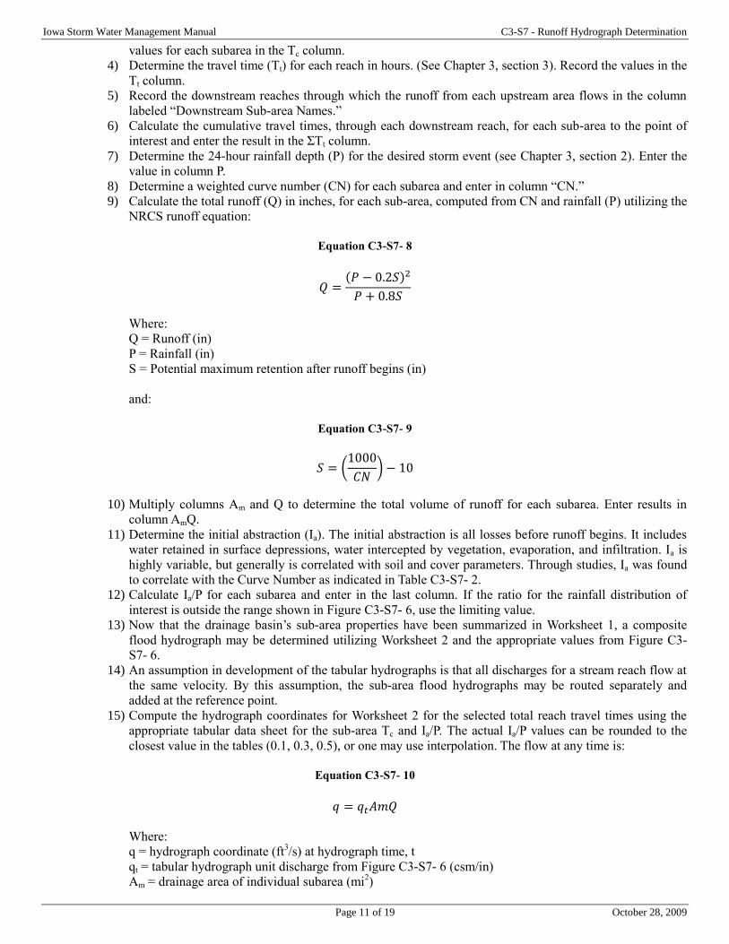
Iowa Storm Water Management Manual C3-S7 - Runoff Hydrograph Determination
Page 11 of 19 October 28, 2009
values for each subarea in the Tc column.
4) Determine the travel time (Tt) for each reach in hours. (See Chapter 3, section 3). Record the values in the
Tt column.
5) Record the downstream reaches through which the runoff from each upstream area flows in the column
labeled “Downstream Sub-area Names.”
6) Calculate the cumulative travel times, through each downstream reach, for each sub-area to the point of
interest and enter the result in the ΣTt column.
7) Determine the 24-hour rainfall depth (P) for the desired storm event (see Chapter 3, section 2). Enter the
value in column P.
8) Determine a weighted curve number (CN) for each subarea and enter in column “CN.”
9) Calculate the total runoff (Q) in inches, for each sub-area, computed from CN and rainfall (P) utilizing the
NRCS runoff equation:
Equation C3-S7- 8
𝑄 =(𝑃 − 0.2𝑆)2
𝑃 + 0.8𝑆
Where:
Q = Runoff (in)
P = Rainfall (in)
S = Potential maximum retention after runoff begins (in)
and:
Equation C3-S7- 9
𝑆 = (1000
𝐶𝑁) − 10
10) Multiply columns Am and Q to determine the total volume of runoff for each subarea. Enter results in
column AmQ.
11) Determine the initial abstraction (Ia). The initial abstraction is all losses before runoff begins. It includes
water retained in surface depressions, water intercepted by vegetation, evaporation, and infiltration. Ia is
highly variable, but generally is correlated with soil and cover parameters. Through studies, Ia was found
to correlate with the Curve Number as indicated in Table C3-S7- 2.
12) Calculate Ia/P for each subarea and enter in the last column. If the ratio for the rainfall distribution of
interest is outside the range shown in Figure C3-S7- 6, use the limiting value.
13) Now that the drainage basin’s sub-area properties have been summarized in Worksheet 1, a composite
flood hydrograph may be determined utilizing Worksheet 2 and the appropriate values from Figure C3-
S7- 6.
14) An assumption in development of the tabular hydrographs is that all discharges for a stream reach flow at
the same velocity. By this assumption, the sub-area flood hydrographs may be routed separately and
added at the reference point.
15) Compute the hydrograph coordinates for Worksheet 2 for the selected total reach travel times using the
appropriate tabular data sheet for the sub-area Tc and Ia/P. The actual Ia/P values can be rounded to the
closest value in the tables (0.1, 0.3, 0.5), or one may use interpolation. The flow at any time is:
Equation C3-S7- 10
𝑞 = 𝑞𝑡𝐴𝑚𝑄
Where:
q = hydrograph coordinate (ft3/s) at hydrograph time, t
qt = tabular hydrograph unit discharge from Figure C3-S7- 6 (csm/in)
Am = drainage area of individual subarea (mi2)

Iowa Storm Water Management Manual C3-S7 - Runoff Hydrograph Determination
Page 12 of 19 October 28, 2009
Q = runoff (in)
Since the timing of peak discharge changes with Tc and Tt, interpolation of peak discharge for Tc and Tt
values is not recommended. Interpolation may result in an estimate of peak discharge that would be
invalid because it would be lower than either of the hydrographs. Therefore, round the actual values of Tc
and Tt to values presented in the tabular data (Figure C3-S7- 6). Perform this rounding so that the sum of
the selected table values is close to the sum of actual Tc and Tt. An acceptable procedure is to select the
results of one of three rounding operations:
Round Tc and Tt separately to the nearest table value and sum
Round Tc down and Tt up to nearest table value and sum
Round Tc up and Tt down to nearest table value and sum.
Transfer the necessary information for each subarea from Worksheet 1 over to Worksheet 2 (Tc, ΣTt, Ia/P,
& AmQ). Enter a consecutive series of hydrograph times from Figure C3-S7- 6. Review the unit
discharges in the tables for the various combinations of Tc and Tt, and make a rough estimate of when the
peak flow for the composite section will occur. This value should be in the middle of the time range
entered in the worksheet.
16) For each subarea and hydrograph time, identify the table of hydrograph data (i.e. Figure C3-S7- 6) for the
appropriate values of Tc, Tt, and Ia/P, and find the corresponding unit discharge in csm/in. Multiply this
value by the value shown in the AmQ column, and record the result in the worksheet as the discharge for
that sub-area at the selected hydrograph time. Repeat this process for each hydrograph time and sub-area.
Upon completion, sum each of the time columns to obtain the composite hydrograph at the outlet.
17) Review the values for the composite hydrograph. Ensure that the values rise, reach a maximum, and then
begin to fall to ensure that the time range selected includes the peak discharge.
2. Tabular method limitations. The tabular method is used to determine peak flows and hydrographs within a
watershed. However, its accuracy decreases as the complexity of the watershed increases. If you want to compare
present and developed conditions of a watershed, use the same procedure for estimating Tc for both conditions.
Use the NRCS WinTR-55 (Chapter 3, section 5) or the WinTR-20 program models instead of the tabular method,
if any of the following conditions applies:
Tt is greater than 3 hours (largest Tt in tabular hydrograph data)
Tc is greater than 2 hours (largest Tt in tabular hydrograph data)
Drainage areas of individual subareas differ by a factor of 5 or more
The entire composite flood hydrograph or entire runoff volume is required for detailed flood routings. The
hydrograph based on extrapolation (tabular method) is only an approximation of the entire hydrograph.
Use the full WinTR-55 or WinTR-20 hydrograph routing for determining inflow hydrograph for detention
storage routing design.
The time of peak discharge must be more accurate than that obtained through the tabular method.
The composite flood hydrograph should be compared with actual stream gage data where possible. The instantaneous
peak flow value from the composite flood hydrograph can be compared with data from USGS curves of peak flow versus
drainage area.
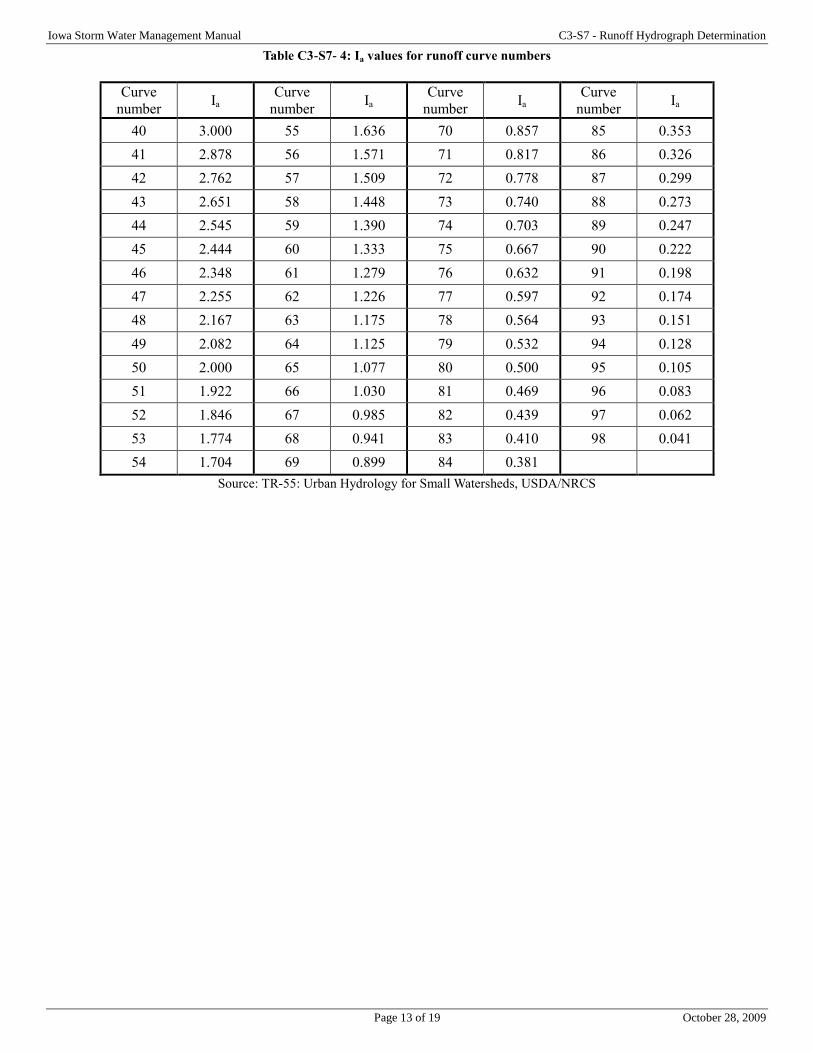
Iowa Storm Water Management Manual C3-S7 - Runoff Hydrograph Determination
Page 13 of 19 October 28, 2009
Table C3-S7- 4: Ia values for runoff curve numbers
Curve
number Ia
Curve
number Ia
Curve
number Ia
Curve
number Ia
40 3.000 55 1.636 70 0.857 85 0.353
41 2.878 56 1.571 71 0.817 86 0.326
42 2.762 57 1.509 72 0.778 87 0.299
43 2.651 58 1.448 73 0.740 88 0.273
44 2.545 59 1.390 74 0.703 89 0.247
45 2.444 60 1.333 75 0.667 90 0.222
46 2.348 61 1.279 76 0.632 91 0.198
47 2.255 62 1.226 77 0.597 92 0.174
48 2.167 63 1.175 78 0.564 93 0.151
49 2.082 64 1.125 79 0.532 94 0.128
50 2.000 65 1.077 80 0.500 95 0.105
51 1.922 66 1.030 81 0.469 96 0.083
52 1.846 67 0.985 82 0.439 97 0.062
53 1.774 68 0.941 83 0.410 98 0.041
54 1.704 69 0.899 84 0.381
Source: TR-55: Urban Hydrology for Small Watersheds, USDA/NRCS

Iowa Storm Water Management Manual C3-S7 - Runoff Hydrograph Determination
Page 14 of 19 October 28, 2009
Worksheet 1: Subarea Properties
Source: TR-55: Urban Hydrology for Small Watersheds, USDA/NRCS

Iowa Storm Water Management Manual C3-S7 - Runoff Hydrograph Determination
Page 15 of 19 October 28, 2009
Worksheet 2: Composite Hydrograph Development
Source: TR-55: Urban Hydrology for Small Watersheds, USDA/NRCS
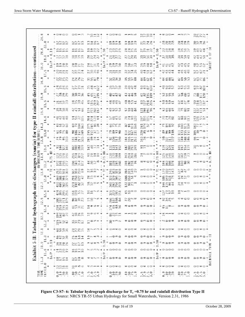
Iowa Storm Water Management Manual C3-S7 - Runoff Hydrograph Determination
Page 16 of 19 October 28, 2009
Figure C3-S7- 6: Tabular hydrograph discharge for Tc =0.75 hr and rainfall distribution Type II
Source: NRCS TR-55 Urban Hydrology for Small Watersheds, Version 2.31, 1986

Iowa Storm Water Management Manual C3-S7 - Runoff Hydrograph Determination
Page 17 of 19 October 28, 2009
F. Design example
Watershed Hydrograph Routing
A new residential development, Hickory Hills, is proposed being proposed for a rural site in Dallas County, IA. A map of
the local watershed in shown in Figure C3-S7- 7 with the development site located in subareas 5, 6, and 7.
Figure C3-S7- 7: Watershed sub-areas for tabular hydrograph Example
Source: Adapted from NRCS TR-55, 1986, version 2.31 user manual, Chapter 5
Compute the peak discharge for the watershed outlet for the developed condition. The basic subarea data for the watershed
is entered into Worksheet 2, and is shown in Worksheet 3. The subarea data for Tc, the summation of travel time to the
outlet for each subarea, and Ia/P values, and the AmQ values have been transferred over to Worksheet 2 shown in
Worksheet 4.
Entry of the hydrograph discharge values in Worksheet 2 is determined as follows:
1. For subarea 6 and using the tabular data in Figure C3-S7- 6 for Tc = 0.75 hr, Tt of 0, and Ia/P value of 0.1 (rounded
up).
2. The unit peak discharge is 424 csm/in and occurs at the hydrograph time (t) of 12.6 hour. The unit peak discharge
is multiplied times the AmQ value for subarea 6 to complete the calculation of the runoff discharge in ft3/sec for
this time. The final computed value is 411 ft3/sec. The remaining hydrograph values for subarea 6 for the other
hydrograph times are completed. In this example, the same data sheet can be used for subarea 4 which has a Tc of
0.75 hour. However, for this subarea, the travel time is 1.5 hour; the hydrograph peak for subarea 4 is 207 ft3/sec,
and occurs at time 14 hours. (For the hydrograph data for the remaining subareas is obtained from the additional
tabular data sheets for rainfall distribution Type 11 and additional Tc’s). The values in this example are extracted
from those sheets to provide a complete routing for this example.
3. The individual discharges are summed for each hydrograph time to give the final composite runoff hydrograph for
the watershed. The total peak discharge at the outlet is 965 ft3/sec, and occurs at 13 hours.
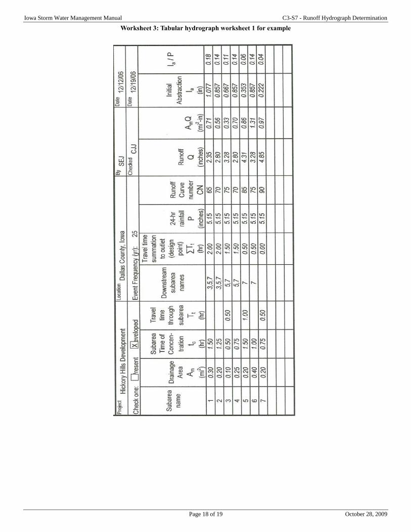
Iowa Storm Water Management Manual C3-S7 - Runoff Hydrograph Determination
Page 18 of 19 October 28, 2009
Worksheet 3: Tabular hydrograph worksheet 1 for example
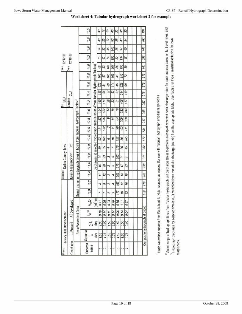
Iowa Storm Water Management Manual C3-S7 - Runoff Hydrograph Determination
Page 19 of 19 October 28, 2009
Worksheet 4: Tabular hydrograph worksheet 2 for example

Page 1 of 21 October 28, 2009
Chapter 3- Section 8 Low-Impact Development (LID) Hydrology
A. Introduction
This section presents a brief summary of low-impact development (LID) hydrologic analysis and computational
procedures used to determine low-impact development stormwater management requirements. The hydrologic analysis
used for the initial development of these procedures is based on the Natural Resources Conservation Service (NRCS) TR-
55 hydrologic model (NRCS, 1986). As described in Chapter 3, section 5, TR-55 was updated to WinTR-55 in 2004.
WinTR-55 now uses the TR-20 computation for rainfall analysis and hydrograph routing. However, the basic underlying
hydrology concepts of CN, time of concentration, peak flow estimation, and determination of runoff volume and storage
remain part of the program (albeit under a different user interface). The material presented here is a summary of the LID
hydrologic analysis principles. The US EPA has published a two-volume manual for low-impact development which is
available at http://www.epa.gov/nps/lid_hydr.pdf. Additional information is also available from the Low-Impact
Development Center at http://www.lowimpactdevelopment.org/. Additional discussion of the LID design approach is
included in Chapter 1 and Chapter 4 of this manual.
Additional discussion of the LID design approach is included in Chapter 1 and Chapter 4 of this manual.
The LID approach attempts to match the pre-development condition by compensating for losses of rainfall abstraction
through maintenance of infiltration potential, evapotranspiration, and surface storage; as well as increased travel time to
reduce rapid concentration of excess runoff. These hydrologic principles were discussed in detail in Chapter 3, section 2
through section 6. Several planning considerations, combined with supplemental controls using LID integrated
management practices, can be used to compensate for rainfall abstraction losses and changes in runoff concentration due
to site development.
B. Hydrologic comparison: conventional vs. low-impact development
Conventional stormwater conveyance systems have traditionally been designed to collect, convey, and discharge runoff as
efficiently as possible. Conventional stormwater management controls are typically sited at the most downstream point of
the entire site (end-of-pipe control). The stormwater management requirement is usually to maintain the peak runoff rates
at pre-development levels for a particular design storm event (typically the Q5 pre-development runoff in most Iowa
jurisdictions). This level of control is called overbank flooding in the unified sizing criteria (see Chapter 2). Therefore,
especially where a stormwater management pond is constructed, the peak flow will not be fully controlled for those storm
events that are less severe than the design storm event. The smaller storms associated with the WQv and Cpv are not
retained in the traditional management approach.
Low-impact development approaches on the other hand, will fully control these storm events, and there is significant
difference between the two approaches. Application of the unified sizing criteria in Chapter 2 can be considered a LID
approach with respect to the size and frequency of storm events captured. Figure C3-S8- 1 illustrates the hydrologic
response of the runoff hydrograph to conventional integrated management practices.
Hydrograph 1 represents the response to a given storm of a site in a pre-development condition (i.e., woods,
meadow). The hydrograph is defined by a gradual rise and fall of the peak discharge and volume.
Hydrograph 2 represents a post-development condition with conventional stormwater BMPs, such as a standard
dry detention pond. Although the peak runoff rate is maintained at the pre- development level, the hydrograph
exhibits significant increases in the runoff volume and duration of runoff from the re-development condition.
Hydrograph 3 represents the response of post-development condition that incorporates low-impact development
stormwater management. Low-impact development uses undisturbed areas and onsite and distributed retention
storage to reduce to reduce runoff volume. The peak runoff rate and volume remain the same as the pre-
development condition through the use of onsite retention and/or detention. The frequency and duration of the
runoff rate are also much closer to the existing condition than those typical of conventional BMPs.
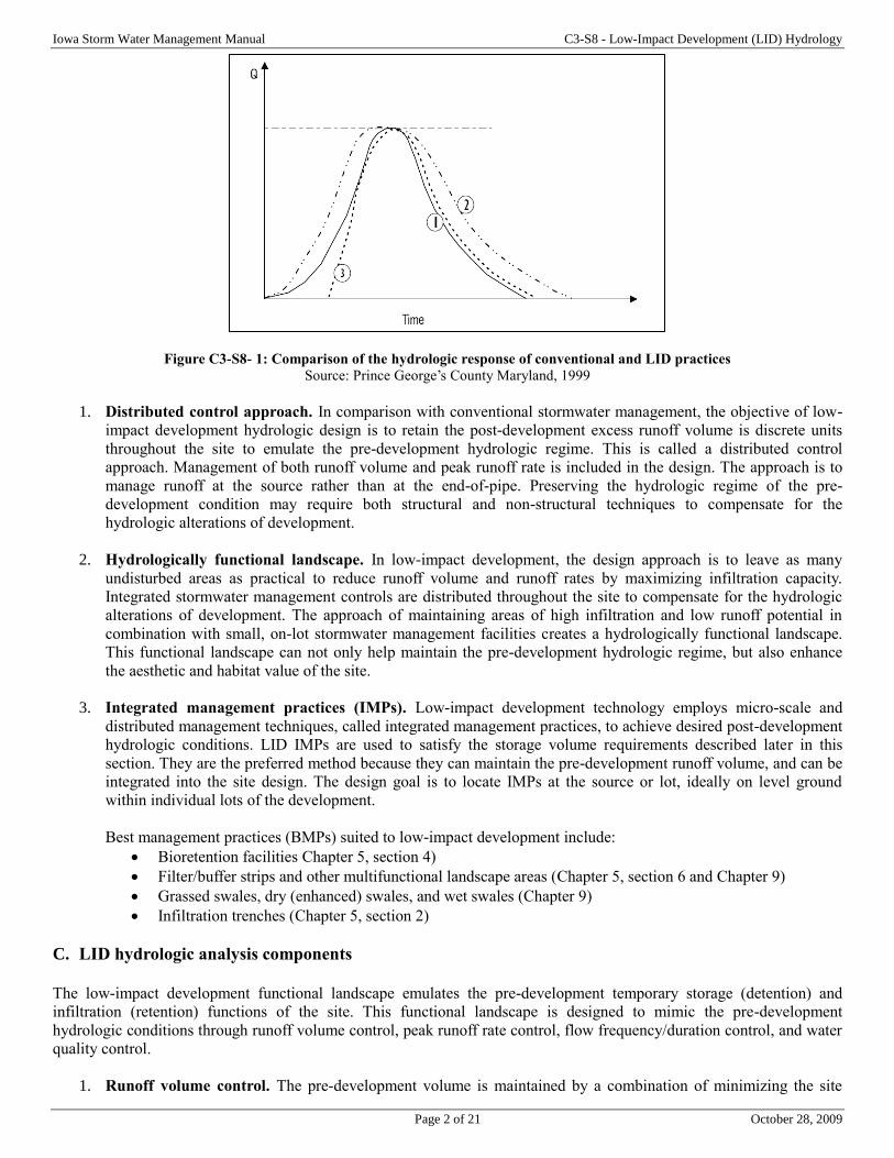
Iowa Storm Water Management Manual C3-S8 - Low-Impact Development (LID) Hydrology
Page 2 of 21 October 28, 2009
Figure C3-S8- 1: Comparison of the hydrologic response of conventional and LID practices
Source: Prince George’s County Maryland, 1999
1. Distributed control approach. In comparison with conventional stormwater management, the objective of low-
impact development hydrologic design is to retain the post-development excess runoff volume is discrete units
throughout the site to emulate the pre-development hydrologic regime. This is called a distributed control
approach. Management of both runoff volume and peak runoff rate is included in the design. The approach is to
manage runoff at the source rather than at the end-of-pipe. Preserving the hydrologic regime of the pre-
development condition may require both structural and non-structural techniques to compensate for the
hydrologic alterations of development.
2. Hydrologically functional landscape. In low-impact development, the design approach is to leave as many
undisturbed areas as practical to reduce runoff volume and runoff rates by maximizing infiltration capacity.
Integrated stormwater management controls are distributed throughout the site to compensate for the hydrologic
alterations of development. The approach of maintaining areas of high infiltration and low runoff potential in
combination with small, on-lot stormwater management facilities creates a hydrologically functional landscape.
This functional landscape can not only help maintain the pre-development hydrologic regime, but also enhance
the aesthetic and habitat value of the site.
3. Integrated management practices (IMPs). Low-impact development technology employs micro-scale and
distributed management techniques, called integrated management practices, to achieve desired post-development
hydrologic conditions. LID IMPs are used to satisfy the storage volume requirements described later in this
section. They are the preferred method because they can maintain the pre-development runoff volume, and can be
integrated into the site design. The design goal is to locate IMPs at the source or lot, ideally on level ground
within individual lots of the development.
Best management practices (BMPs) suited to low-impact development include:
Bioretention facilities Chapter 5, section 4)
Filter/buffer strips and other multifunctional landscape areas (Chapter 5, section 6 and Chapter 9)
Grassed swales, dry (enhanced) swales, and wet swales (Chapter 9)
Infiltration trenches (Chapter 5, section 2)
C. LID hydrologic analysis components
The low-impact development functional landscape emulates the pre-development temporary storage (detention) and
infiltration (retention) functions of the site. This functional landscape is designed to mimic the pre-development
hydrologic conditions through runoff volume control, peak runoff rate control, flow frequency/duration control, and water
quality control.
1. Runoff volume control. The pre-development volume is maintained by a combination of minimizing the site

Iowa Storm Water Management Manual C3-S8 - Low-Impact Development (LID) Hydrology
Page 3 of 21 October 28, 2009
disturbance from the pre-development condition and providing distributed BMPs to capture and retain rainfall on
the landscape. These BMPs are structures that capture and retain the WQv, and perhaps the Cpv runoff for the
design storm event.
2. Peak runoff rate control. Low-impact development is designed to maintain the pre- development peak runoff
discharge rate for the selected design storm events. This is done by maintaining the pre-development Tc and then
using retention and/or detention BMPs (e.g., rain gardens, bioretention, open drainage systems, etc.) that are
distributed throughout the site. The goal is to use retention practices to control runoff volume and, if these
retention practices are not sufficient to control the peak runoff rate, to use additional detention practices to control
the peak runoff rate. Detention is temporary storage that releases excess runoff at a controlled rate. The use of
retention and detention to control the peak runoff rate is defined as the hybrid approach.
3. Flow frequency/duration control. Since low-impact development is designed to emulate the pre-development
hydrologic regime through both volume and peak runoff rate controls, the flow frequency and duration for the
post-development conditions will be almost identical to those for the pre-development conditions. The impacts on
the sediment and erosion and stream habitat potential at downstream reaches can then be minimized.
4. Water quality control. Low-impact development is designed to provide water quality treatment control for the
first ½ inch of runoff from impervious areas using retention practices. This is equivalent to the WQv criteria in
Chapter 2 where the WQv design storm is 1.25 inches. For a development site with 40% impervious area, the Rv
would be 0.41 and the runoff volume captured as the WQv would be 0.51 inches.
The low-impact analysis and design approach focuses on the following hydrologic analysis and design
components:
Runoff curve number (CN). Minimizing change in post-development hydrology by reducing impervious
areas and preserving more trees and meadows to reduce the storage requirements to maintain the pre-
development runoff volume.
Time of concentration (Tc). Maintaining the pre-development Tc in order to minimize the increase of the
peak runoff rate after development by lengthening flow paths and reducing the length of the runoff
conveyance systems.
Retention. Providing retention storage for volume and peak control, as well as water quality control, to
maintain the same storage volume as the pre-development condition.
Detention. Providing additional detention storage, if required, to maintain the same peak runoff rate
and/or prevent flooding for storm recurrence intervals ≥5-10 years.
The LID design objectives listed above are carried out through application of basic hydrologic principles related
to rainfall and runoff analysis. The current capabilities in WinTR-55 allow for the user development and user
input of Custom CN’s based on a careful analysis of the site conditions. Development and design practices for
implementing the hydrologic controls above are summarized in Table C3-S8- 1.

Iowa Storm Water Management Manual C3-S8 - Low-Impact Development (LID) Hydrology
Page 4 of 21 October 28, 2009
Table C3-S8- 1: Low-impact development techniques and hydrologic design and analysis techniques
Source: Prince George’s County Maryland, 1999
D. Process and computational procedure
The hydrologic analysis of low-impact development is a sequential decision-making process, and is illustrated in Figure
C3-S8- 2. Several iterations may occur within each step until the appropriate approach to reduce stormwater impacts is
determined. The procedures for each step are summarized below. A set of design charts have been developed to determine
the amount of storage required to maintain the existing volume and peak runoff rates to satisfy jurisdictional requirements
for stormwater management requirements. The full set of charts is not included in this manual, but examples of each of the
three types of charts (Figure C3-S8- 3, Figure C3-S8- 4, and Figure C3-S8- 5) are provided so the design process can be
illustrated. The full set of manuals, including “Low-Impact Development Design Strategies: An Integrated Design
Approach” (EPA 841-B-00-003) and “Low-Impact Development Hydrologic Analysis” (EPA 841-B-00-002) are available
at http://www.lowimpactdevelopment.org/publications.htm. The full set of design charts is available from the Prince
George’s County Maryland DER.
The procedure is summarized below and the sequence is portrayed graphically in Figure C3-S8- 2.
1. Data collection. The basic information used to develop the low-impact development site plan and used to
determine the runoff curve number (CN) and time of concentration (Tc) for the pre- and post-development
condition is the same as conventional site plan and stormwater management approaches discussed earlier in the
section.
2. Determining the LID runoff curve number. The determination of the low-impact development CN requires a
detailed evaluation of each land cover within the development site. The goal is to take full advantage of the
storage and infiltration characteristics of low-impact development site planning to maintain the CN. The LID
approach encourages the conservation and creation of more open grassland and wooded areas, and the reduction
of impervious area to minimize the need for extensive piped drainage. The steps for determining the low-impact
development CN are as follows:
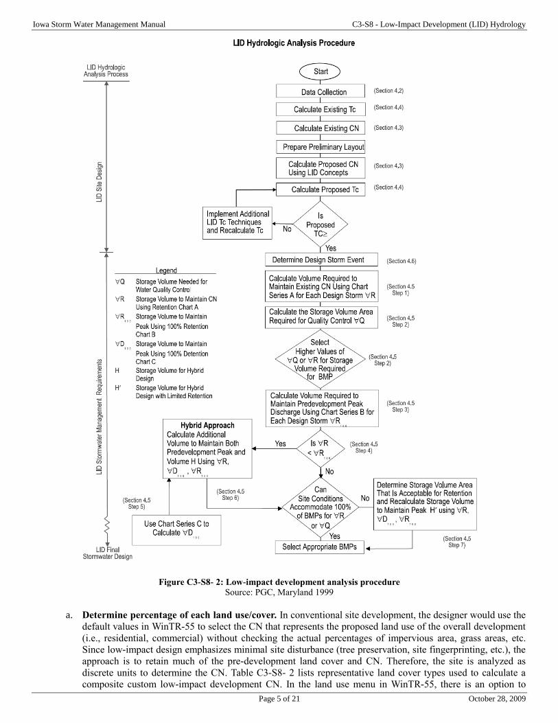
Iowa Storm Water Management Manual C3-S8 - Low-Impact Development (LID) Hydrology
Page 5 of 21 October 28, 2009
Figure C3-S8- 2: Low-impact development analysis procedure
Source: PGC, Maryland 1999
a. Determine percentage of each land use/cover. In conventional site development, the designer would use the
default values in WinTR-55 to select the CN that represents the proposed land use of the overall development
(i.e., residential, commercial) without checking the actual percentages of impervious area, grass areas, etc.
Since low-impact design emphasizes minimal site disturbance (tree preservation, site fingerprinting, etc.), the
approach is to retain much of the pre-development land cover and CN. Therefore, the site is analyzed as
discrete units to determine the CN. Table C3-S8- 2 lists representative land cover types used to calculate a
composite custom low-impact development CN. In the land use menu in WinTR-55, there is an option to
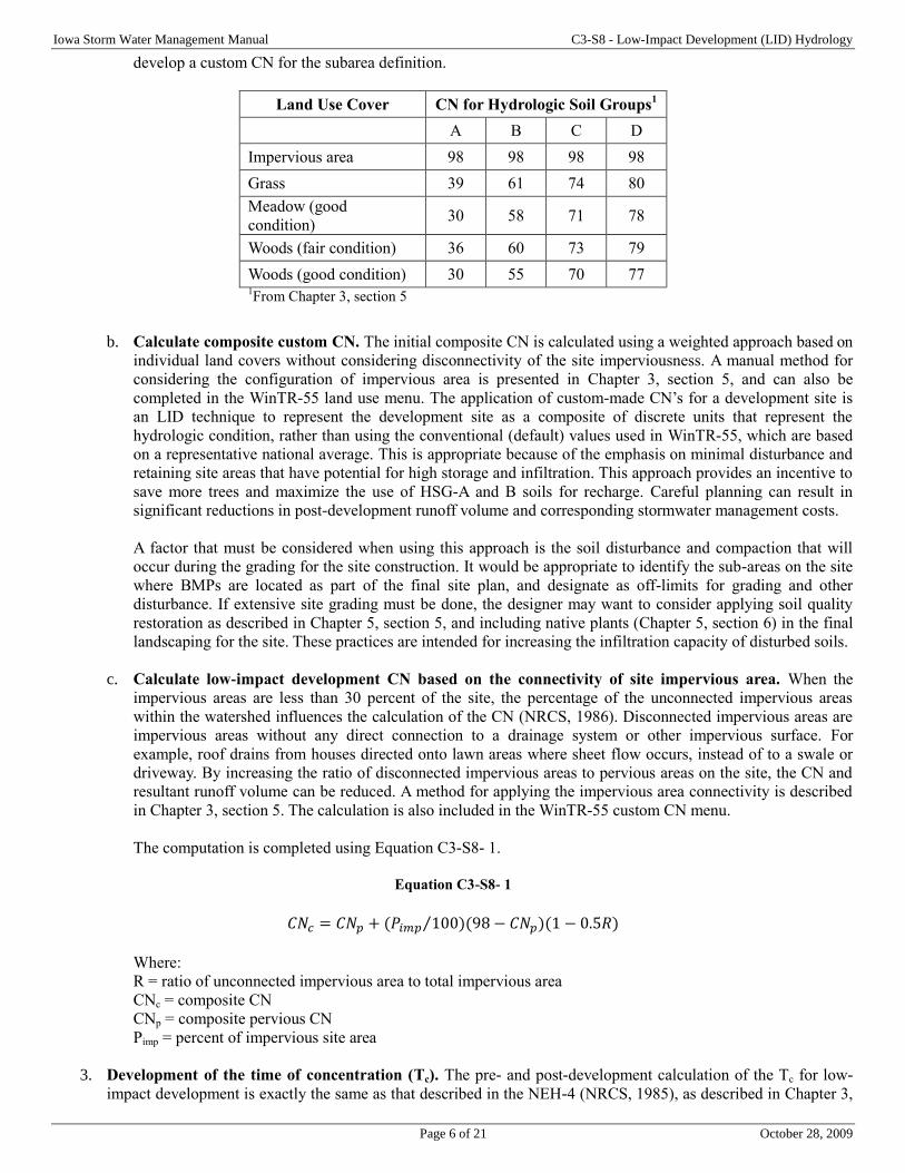
Iowa Storm Water Management Manual C3-S8 - Low-Impact Development (LID) Hydrology
Page 6 of 21 October 28, 2009
develop a custom CN for the subarea definition.
Land Use Cover CN for Hydrologic Soil Groups1
A B C D
Impervious area 98 98 98 98
Grass 39 61 74 80
Meadow (good
condition) 30 58 71 78
Woods (fair condition) 36 60 73 79
Woods (good condition) 30 55 70 77 1From Chapter 3, section 5
b. Calculate composite custom CN. The initial composite CN is calculated using a weighted approach based on
individual land covers without considering disconnectivity of the site imperviousness. A manual method for
considering the configuration of impervious area is presented in Chapter 3, section 5, and can also be
completed in the WinTR-55 land use menu. The application of custom-made CN’s for a development site is
an LID technique to represent the development site as a composite of discrete units that represent the
hydrologic condition, rather than using the conventional (default) values used in WinTR-55, which are based
on a representative national average. This is appropriate because of the emphasis on minimal disturbance and
retaining site areas that have potential for high storage and infiltration. This approach provides an incentive to
save more trees and maximize the use of HSG-A and B soils for recharge. Careful planning can result in
significant reductions in post-development runoff volume and corresponding stormwater management costs.
A factor that must be considered when using this approach is the soil disturbance and compaction that will
occur during the grading for the site construction. It would be appropriate to identify the sub-areas on the site
where BMPs are located as part of the final site plan, and designate as off-limits for grading and other
disturbance. If extensive site grading must be done, the designer may want to consider applying soil quality
restoration as described in Chapter 5, section 5, and including native plants (Chapter 5, section 6) in the final
landscaping for the site. These practices are intended for increasing the infiltration capacity of disturbed soils.
c. Calculate low-impact development CN based on the connectivity of site impervious area. When the
impervious areas are less than 30 percent of the site, the percentage of the unconnected impervious areas
within the watershed influences the calculation of the CN (NRCS, 1986). Disconnected impervious areas are
impervious areas without any direct connection to a drainage system or other impervious surface. For
example, roof drains from houses directed onto lawn areas where sheet flow occurs, instead of to a swale or
driveway. By increasing the ratio of disconnected impervious areas to pervious areas on the site, the CN and
resultant runoff volume can be reduced. A method for applying the impervious area connectivity is described
in Chapter 3, section 5. The calculation is also included in the WinTR-55 custom CN menu.
The computation is completed using Equation C3-S8- 1.
Equation C3-S8- 1
𝐶𝑁𝑐 = 𝐶𝑁𝑝 + (𝑃𝑖𝑚𝑝 100)(98 − 𝐶𝑁𝑝)(1 − 0.5𝑅)⁄
Where:
R = ratio of unconnected impervious area to total impervious area
CNc = composite CN
CNp = composite pervious CN
Pimp = percent of impervious site area
3. Development of the time of concentration (Tc). The pre- and post-development calculation of the Tc for low-
impact development is exactly the same as that described in the NEH-4 (NRCS, 1985), as described in Chapter 3,
Iowa Storm Water Management Manual C3-S8 - Low-Impact Development (LID) Hydrology
Page 7 of 21 October 28, 2009
section 3, and computed with WinTR-55.
4. Low-impact development stormwater management requirements. Once the CN and Tc are determined for the
pre- and post-development conditions, the stormwater management storage volume requirements can be
calculated. The low-impact development objective is to create enough runoff retention capacity onsite to maintain
all the pre-development volume, pre- development peak runoff rate, and frequency. In the LID procedure, the
required runoff retention capacity is termed “storage,” even though this includes all of processes that abstract
rainfall after a rainfall event. In traditional terms, the storage is equal to the term “S” in the NRCS rainfall-runoff
equation (Chapter 3, section 5) and includes infiltration. This may be accomplished through application of a series
of non-structural and structural BMPs, including detention practices. By adding onsite practices to increase
infiltration, the site storage value for “S” in the rainfall-runoff relationship is increased. The required storage
volume is calculated using the design charts in Figure C3-S8- 3, Figure C3-S8- 4, and Figure C3-S8- 5. The
required storage volume is heavily dependent on the rainfall intensity (rainfall distribution). Rainfall intensity
varies considerably over geographic regions in the US, and the standard NRCS Type II distribution is used in
Iowa (Chapter 3, section 1). The remaining low- impact development hydrologic analysis techniques are based on
the premise that the post- development Tc is the same as the pre-development condition. If the post-development
Tc does not equal the pre-development Tc, additional low-impact development site design techniques must be
implemented to maintain the Tc. However, the final site hydrologic design after the application of all
recommended BMPs should be based on the actual Tc achieved.
Three series of design charts are needed to determine the storage volume required to control the increase in runoff
volume and peak runoff rate using retention and detention practices. The required storages shown in these design
charts are presented as a depth in hundredths of an inch (over the development site). Equation C3-S8- 2 is used to
determine the volume required for IMPs.
Equation C3-S8- 2
𝑉𝑜𝑙𝑢𝑚𝑒(𝑖𝑛) = (𝑑𝑒𝑝𝑡ℎ 𝑓𝑟𝑜𝑚 𝑑𝑒𝑠𝑖𝑔𝑛 𝑐ℎ𝑎𝑟𝑡 − 𝑖𝑛) ×𝑑𝑒𝑣𝑒𝑙𝑜𝑝𝑚𝑒𝑛𝑡 𝑠𝑖𝑧𝑒 − 𝑎𝑐
100
A 6-inch depth is the recommended maximum depth for bioretention basins used in low-impact development. The
amount, or depth, of exfiltration of the runoff by infiltration or by the process of evapotranspiration is not
included in the design charts. Reducing surface area requirements through the consideration of these factors can
be determined by using Equation C3-S8- 3.
Equation C3-S8- 3
𝑉𝑜𝑙𝑢𝑚𝑒 𝑜𝑓 𝑠𝑖𝑡𝑒 𝑎𝑟𝑒𝑎 𝑓𝑜𝑟 𝐼𝑀𝑃𝑠 = (𝑖𝑛𝑖𝑡𝑖𝑎𝑙 𝑣𝑜𝑙𝑢𝑚𝑒) ×100 − 𝑥
100
Where:
x = % of the storage volume infiltrated and/or reduced by evaporation or transpiration
x% should be minimal (less than 10%)
Stormwater management is accomplished by selecting the appropriate BMP, or combination of BMPs, to satisfy
the surface area and volume requirements calculated from using the design charts. The design charts to be used to
evaluate these requirements are:
Chart Series A: Storage volume required for maintaining the pre-development runoff volume using
retention storage (Figure C3-S8- 4 and Figure C3-S8- 5).
Chart Series B: Storage volume required for maintaining the pre-development peak runoff rate using
100% retention (Figure C3-S8- 4).
Chart Series C: Storage volume required for maintaining the pre-development peak runoff rate using
100% detention (Figure C3-S8- 5).
The charts are based on the following general conditions:
The land uses for the development are relatively homogeneous throughout the site.
Iowa Storm Water Management Manual C3-S8 - Low-Impact Development (LID) Hydrology
Page 8 of 21 October 28, 2009
The stormwater management measures are to be distributed evenly across the development, to the greatest
extent possible.
The design storm is based on 1-inch increments. Use linear interpolation for determining intermediate
values.
E. Determination of design storm event As discussed previously in Chapter 1, Chapter 2, and Chapter 3, section 6, conventional stormwater management runoff
quantity control is generally based on not exceeding the pre-development peak runoff rate for the 2-year/5-year and 10-
year, 24-hour Type II storm events. The amount of rainfall used to determine the runoff for the site is derived from the
Midwest Rainfall Atlas (Bulletin 71) rainfalls provided in Table C3-S2- 2 and Table C3-S2- 3. As an example, the 2-year
and 10-year, 24-hour storm events for Climate District 5 (Central Iowa) are 2.91 and 4.27 inches, respectively. In the
unified sizing criteria (Chapter 2), the design storm for the WQv is established at 1.25 inches, and the design storm for
Cpv is the 1-year, 24-hour duration rainfall. The WQv design rainfall is considered to be a statewide value. The 1-year,
24-hour rainfall for central Iowa is 2.38 inches. The 5-year and 10-year events are typically used for sizing of stormwater
conveyance inlets and piping.
For low-impact development, the design storm is based on the goal of maintaining the pre- development hydrologic
conditions for the site. The determination of the design storm begins with an evaluation of the pre-development condition.
The hydrologic approach of low-impact development is to retain the same amount of rainfall within the development site
as that which is retained by meadow in good condition, and then to gradually release the excess runoff as a grassland
meadow would release it. The predominant landscape condition in Iowa before development was native prairie, and a
meadow in good condition would be the best land condition comparison. By using this approach, the final design will
emulate, to the greatest extent practical, the pre-development hydrologic regime to protect watershed and natural habitats.
Therefore, the pre-development condition of the low-impact development site is required to be meadow in good condition.
Note that a pre-development condition of row-crop agriculture is not undeveloped in a hydrologic sense. In some cases,
residential development on a pre-existing site with row-crop land use can actually show a decrease in CN from the pre-
development condition. This is consistent with the pre-development condition described in Chapter 2. The design storm
will be the greater of the rainfall at which direct runoff begins from a meadow in good condition with a modifying factor,
or the 1-year, 24-hour storm event. The rainfall at which direct runoff begins is determined using Equation C3-S8- 4.
Equation C3-S8- 4
𝑃 = 0.2 (1000
𝐶𝑁𝑐− 10)
P is the rainfall at which direct runoff begins. This is the same relationship used in the NRCS runoff equation to compute
the runoff in inches from a given rainfall depth and watershed CN.
Step 1: Determine the pre-development CN. Use an existing land cover of meadow in good condition overlaid
over the hydrologic soils group (HSG) to determine the composite site CN.
Step 2: Determine the amount of rainfall needed to initiate direct runoff. Use Equation C3-S8- 4 to determine
the amount of rainfall (P) needed to initiate direct runoff.
Step 3: Account for variation in land cover. Multiply the amount of rainfall (P) determined in Step 2 by a factor
of 1.5.
Example:
A site is 70% HSG-B and 30% HSG-C soils. The CN’s for meadow in good condition for HSG-B and HSG-C
soils are 58 and 71, respectively (From Chapter 3, section 5).
CNc = (0,70)(58) + (0.30)(71) = 61.9 Use 62
Determine the rainfall amount to initiate runoff: P = 0.2 (1000/62-10) = 1.22 inches
Multiply by rainfall amount by a factor of 1.5: Design rainfall = 1,22 in x 1.5 = 1.83 inches
The procedure to determine the BMP requirements is outlined in Figure C3-S8- 3. A summary description is
described below.
1. Step 1: Determine storage volume required to maintain pre-development volume or CN using retention
storage. The post-development runoff volume generated as a result of the post-development custom-made CN is

Iowa Storm Water Management Manual C3-S8 - Low-Impact Development (LID) Hydrology
Page 9 of 21 October 28, 2009
compared to the pre-development runoff volume to determine the surface area required for volume control. Use
Chart Series A: Storage volume required to maintain the pre-development runoff volume using retention storage.
The procedure for calculating the site area required for maintaining runoff volume is provided in Example 1. It
should be noted that the practical and reasonable use of the site must be considered. The BMPs must not restrict
the use of the site. The storage area expressed is for runoff volume control only; additional storage may be
required for water quality control. The procedure to account for the water quality volume in the current water
quality requirement is found in Step 2.
Example 1
Given:
Site area = 28 acres
Existing CN = 62
Proposed CN = 68
Design storm is 1.83 inches (round up to 2 inches to use charts)
Design depth of BMP will be 6 inches
Solution: Use Chart Series A: Storage volume required to maintain runoff volume or CN.
From Chart A:
0.11 inch (from Chart A for 2-inch rainfall and CN’s of 62/68) of storage over the site is required to maintain the runoff
volume. Therefore, if 6-inch design depth is used: 0.51 acres (28 acres x 0.11 in/6 in) of BMPs distributed evenly
throughout the site are required to maintain the runoff volume, or CN.
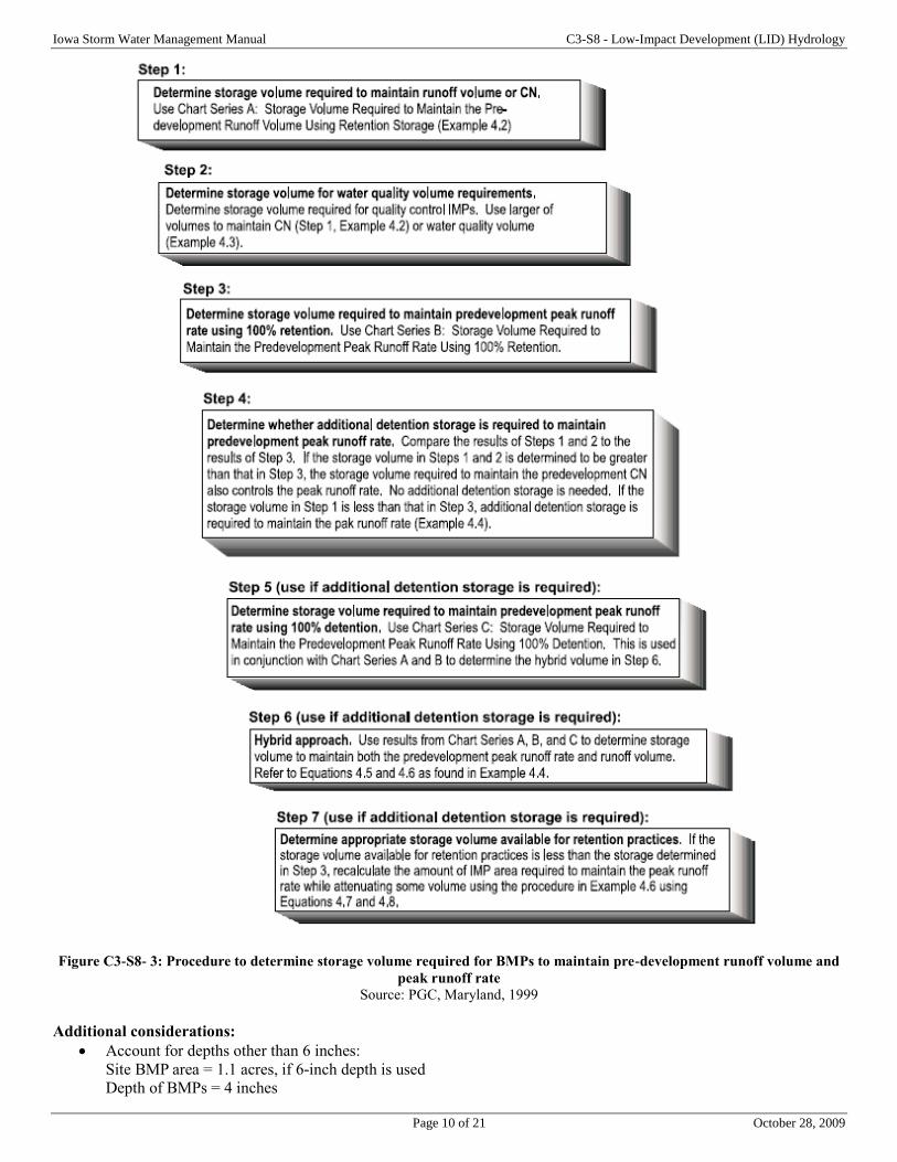
Iowa Storm Water Management Manual C3-S8 - Low-Impact Development (LID) Hydrology
Page 10 of 21 October 28, 2009
Figure C3-S8- 3: Procedure to determine storage volume required for BMPs to maintain pre-development runoff volume and
peak runoff rate
Source: PGC, Maryland, 1999
Additional considerations:
Account for depths other than 6 inches:
Site BMP area = 1.1 acres, if 6-inch depth is used
Depth of BMPs = 4 inches
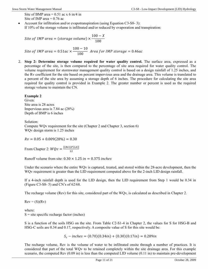
Iowa Storm Water Management Manual C3-S8 - Low-Impact Development (LID) Hydrology
Page 11 of 21 October 28, 2009
Site of BMP area = 0.51 ac x 6 in/4 in
Site of IMP area = 0.76 ac
Account for infiltration and/or evapotranspiration (using Equation C3-S8- 3):
If 10% of the storage volume is infiltrated and/or reduced by evaporation and transpiration:
𝑆𝑖𝑡𝑒 𝑜𝑓 𝐼𝑀𝑃 𝑎𝑟𝑒𝑎 = (𝑠𝑡𝑜𝑟𝑎𝑔𝑒 𝑣𝑜𝑙𝑢𝑚𝑒) ×100 − 𝑋
100
𝑆𝑖𝑡𝑒 𝑜𝑓 𝐼𝑀𝑃 𝑎𝑟𝑒𝑎 = 0.51𝑎𝑐 ×100 − 10
100 𝐴𝑟𝑒𝑎 𝑓𝑜𝑟 𝐼𝑀𝑃 𝑠𝑡𝑜𝑟𝑎𝑔𝑒 = 0.46𝑎𝑐
2. Step 2: Determine storage volume required for water quality control. The surface area, expressed as a
percentage of the site, is then compared to the percentage of site area required for water quality control. The
volume requirement for stormwater management quality control is based on a design rainfall of 1.25 inches, and
the Rv coefficient for the site based on percent impervious area and the drainage area. This volume is translated to
a percent of the site area by assuming a storage depth of 6 inches. The procedure for calculating the site area
required for quality control is provided in Example 2. The greater number or percent is used as the required
storage volume to maintain the CN.
Example 2
Given:
Site area is 28 acres
Impervious area is 7.84 ac (28%)
Depth of BMP is 6 inches
Solution:
Compute WQv requirement for the site (Chapter 2 and Chapter 3, section 6)
WQv design storm is 1.25 inches
𝑅𝑣 = 0.05 + 0.009(28%) = 0.30
From Chapter 2: 𝑊𝑄𝑣 =[(𝑅𝑣)(𝑃)(𝐴)]
12
Runoff volume from site: 0.30 × 1.25 𝑖𝑛 = 0.375 𝑖𝑛𝑐ℎ𝑒𝑠
Under the scenario where the entire WQv is captured, treated, and stored within the 28-acre development, then the
WQv requirement is greater than the LID requirement computed above for the 2-inch LID design rainfall.
If a 4-inch rainfall depth is used for the LID design, then the LID requirement from Step 1 would be 0.34 in
(Figure C3-S8- 5) and CN’s of 62/68.
The recharge volume (Rev) for this site, considered part of the WQv, is calculated as described in Chapter 2.
Rev = (S)(Rv)
where:
S = site specific recharge factor (inches)
S is a function of the soils HSG on the site. From Table C2-S1-4 in Chapter 2, the values for S for HSG-B and
HSG-C soils are 0.34 and 0.17, respectively. A composite value of S for this site would be:
𝑆𝑐 − 𝑖𝑛𝑐ℎ𝑒𝑠 = (0.70)(0.34𝑖𝑛) + (0.30)(0.17𝑖𝑛) = 0.289𝑖𝑛
The recharge volume, Rev is the volume of water to be infiltrated onsite through a number of practices. It is
considered that part of the total WQv to be retained completely within the site drainage area. For this example
scenario, the computed Rev (0.09 in) is less than the computed LID volume (0.11 in) to maintain pre-development
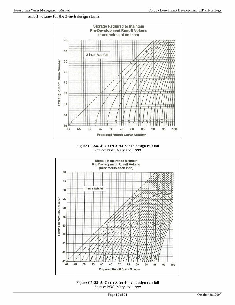
Iowa Storm Water Management Manual C3-S8 - Low-Impact Development (LID) Hydrology
Page 12 of 21 October 28, 2009
runoff volume for the 2-inch design storm.
Figure C3-S8- 4: Chart A for 2-inch design rainfall
Source: PGC, Maryland, 1999
Figure C3-S8- 5: Chart A for 4-inch design rainfall Source: PGC, Maryland, 1999

Iowa Storm Water Management Manual C3-S8 - Low-Impact Development (LID) Hydrology
Page 13 of 21 October 28, 2009
Summary for Step 2: From the results of Example 2, the WQv requirement is 0.37 inches. Of the total WQv
requirement for the site, the recharge volume, Rev, of 0.09 inches would be retained onsite. The remainder of the
WQv could substantially be released after treatment in a BMP. Using the LID volume of 0.11 inches (for a 2-inch
design storm) would meet the requirement to maintain the pre-development runoff volume.
3. Step 3: Determine storage volume required to maintain peak stormwater runoff rate using 100 percent
retention. The percentage of site area or amount of storage required to maintain the pre-development peak runoff
rate is based on Chart Series B: Percentage of site area required to maintain pre-development peak runoff rate
using 100% retention. This chart is based on the relationship between storage volume ratio (Vs/Vr) and discharge
(q0/qi) to maintain the pre-development peak runoff rate.
Where:
Vs = volume of storage required to maintain the pre-development peak runoff rate using 100% retention
Vr = post-development runoff volume
q0 = peak outflow discharge rate (i.e., the peak discharge for the pre-development condition)
qi = peak inflow rate (the peak discharge rate for the post-development condition)
The relationship for retention storage to control the peak runoff rate is similar to the relationship for detention
storage. Figure C3-S8- 6 is an illustration of the comparison of the storage volume/discharge relationship for
retention and detention. Curve A is the relationship of storage volume to discharge to maintain the pre-
development peak runoff rate using the detention relationship. This is the same relationship provided in Chapter 3,
section 6, and is the same principle used in Chapter 3, section 9 for making preliminary estimates of detention
volume for peak rate control. The relationship is based on data prepared for the NRCS TR-55, and is included in
Chapter 6 of the 1986 user’s manual for TR-55. Curve B is the ratio of storage volume to discharge to maintain
the pre-development peak runoff rate using 100 percent retention. Note that the volume required to maintain the
peak runoff rate using detention is less than the requirement for retention. This is graphically demonstrated in
Figure C3-S8- 6. The retention value is larger since the runoff volume is permanently retained onsite while the
detention value is captured and then ultimately released over a set period of time.
The values for Vr, q0, and qi are determined from the WinTR-55 analysis of the pre-development and post-
development scenarios for the site. In this case, the design storm for LID analysis would be manually entered in
the rainfall menu in the program. Using the pre-development and post-development CN and Tc values determined
in Step 2 and Step 3 of the LID procedure, the WinTR-55 analysis is then run for both the pre-development and
post-development scenarios. In WinTR-55, the peak discharge rate and runoff values are accessed in the TR-20
reports menu.
In Figure C3-S8- 6:
Hydrograph 2 represents the runoff response for a post-development condition with no BMPs used on the
site. As discussed in earlier this manual, the post-development hydrograph will generally reflect a shorter
time of concentration, Tc, and the increase in total site imperviousness compared to the pre-development
condition. The hydrograph shows a decrease in the time to peak, Tp, and an increase in peak runoff rate
and total runoff volume, as well as an increased discharge duration.
Hydrograph 8 illustrates the effect of providing additional detention storage to reduce the post-
development peak discharge rate to pre-development conditions.
V1 is the storage volume required to maintain the pre-development peak discharge ratio using 100%
detention storage (See Chapter 3, section 9). The combination of V1 and V2 is the storage volume required
to maintain the pre-development peak rate using 100% retention storage.
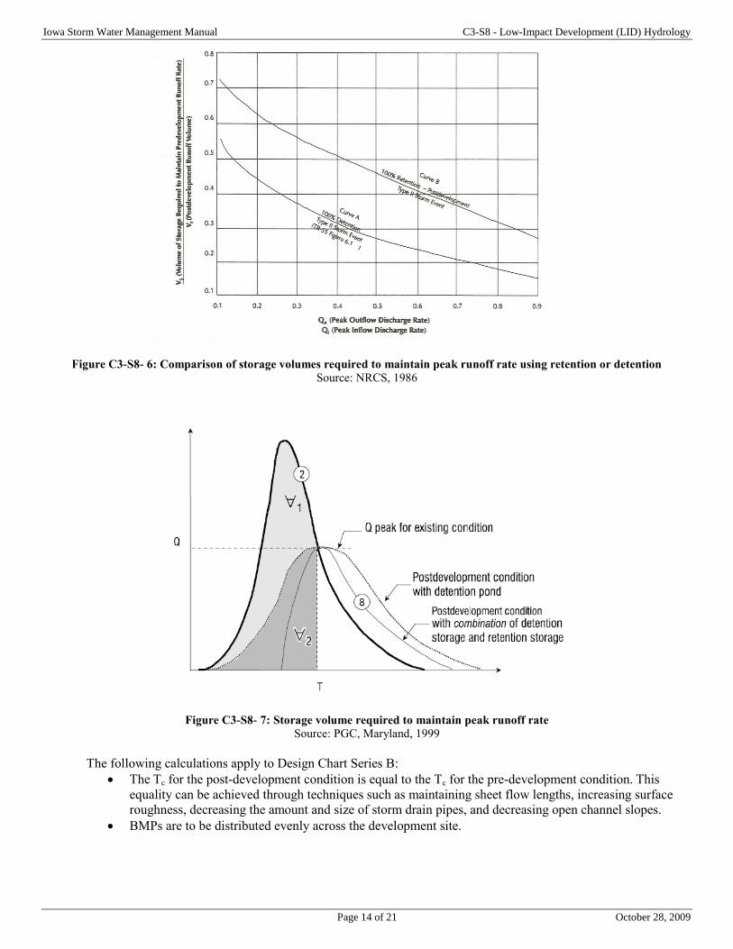
Iowa Storm Water Management Manual C3-S8 - Low-Impact Development (LID) Hydrology
Page 14 of 21 October 28, 2009
Figure C3-S8- 6: Comparison of storage volumes required to maintain peak runoff rate using retention or detention
Source: NRCS, 1986
Figure C3-S8- 7: Storage volume required to maintain peak runoff rate
Source: PGC, Maryland, 1999
The following calculations apply to Design Chart Series B:
The Tc for the post-development condition is equal to the Tc for the pre-development condition. This
equality can be achieved through techniques such as maintaining sheet flow lengths, increasing surface
roughness, decreasing the amount and size of storm drain pipes, and decreasing open channel slopes.
BMPs are to be distributed evenly across the development site.
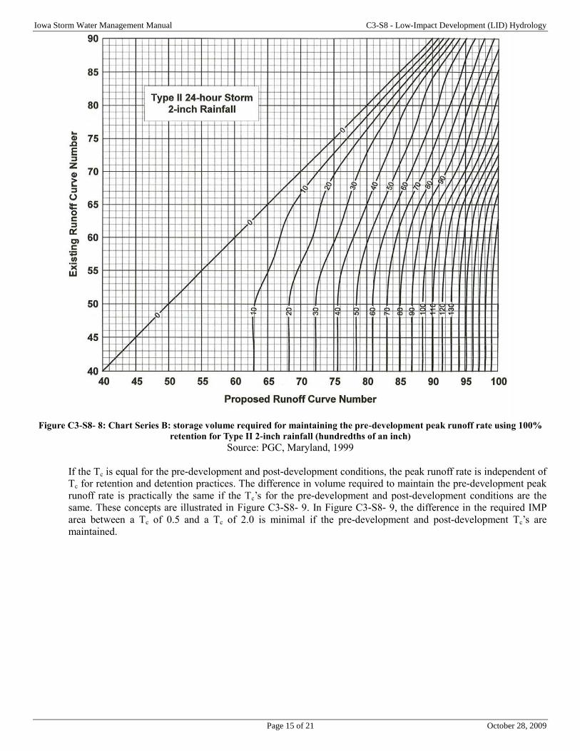
Iowa Storm Water Management Manual C3-S8 - Low-Impact Development (LID) Hydrology
Page 15 of 21 October 28, 2009
Figure C3-S8- 8: Chart Series B: storage volume required for maintaining the pre-development peak runoff rate using 100%
retention for Type II 2-inch rainfall (hundredths of an inch)
Source: PGC, Maryland, 1999
If the Tc is equal for the pre-development and post-development conditions, the peak runoff rate is independent of
Tc for retention and detention practices. The difference in volume required to maintain the pre-development peak
runoff rate is practically the same if the Tc’s for the pre-development and post-development conditions are the
same. These concepts are illustrated in Figure C3-S8- 9. In Figure C3-S8- 9, the difference in the required IMP
area between a Tc of 0.5 and a Tc of 2.0 is minimal if the pre-development and post-development Tc’s are
maintained.
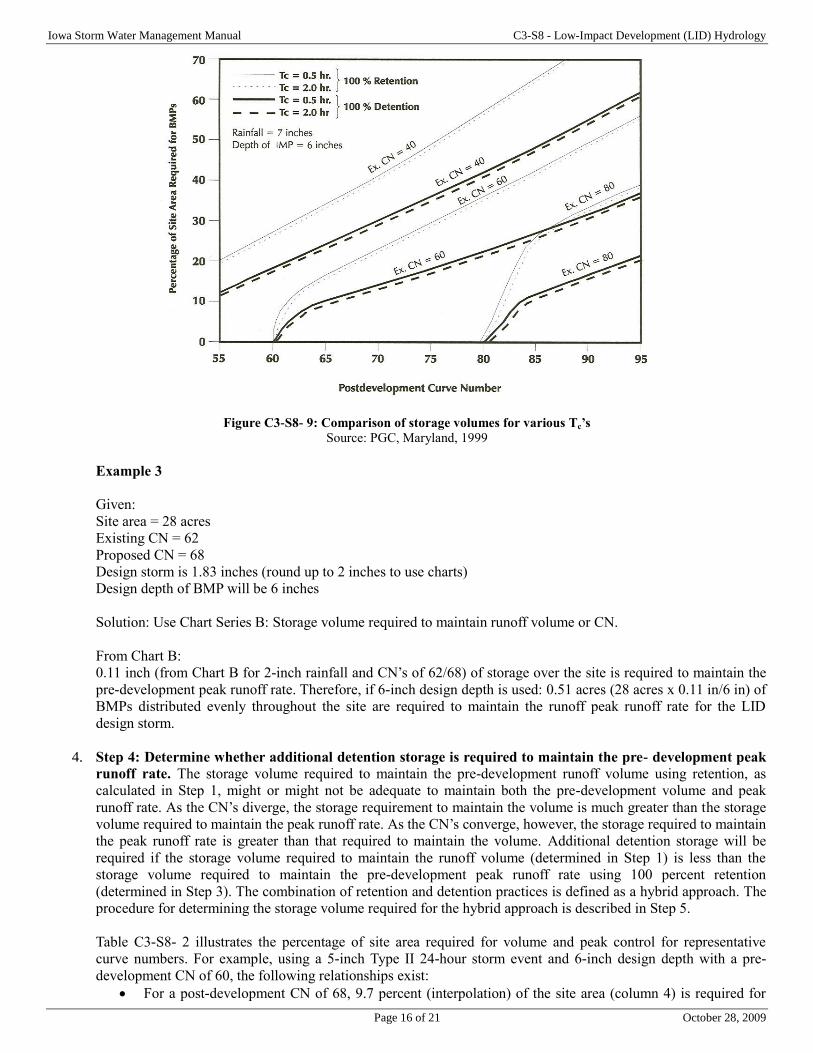
Iowa Storm Water Management Manual C3-S8 - Low-Impact Development (LID) Hydrology
Page 16 of 21 October 28, 2009
Figure C3-S8- 9: Comparison of storage volumes for various Tc’s
Source: PGC, Maryland, 1999
Example 3
Given:
Site area = 28 acres
Existing CN = 62
Proposed CN = 68
Design storm is 1.83 inches (round up to 2 inches to use charts)
Design depth of BMP will be 6 inches
Solution: Use Chart Series B: Storage volume required to maintain runoff volume or CN.
From Chart B:
0.11 inch (from Chart B for 2-inch rainfall and CN’s of 62/68) of storage over the site is required to maintain the
pre-development peak runoff rate. Therefore, if 6-inch design depth is used: 0.51 acres (28 acres x 0.11 in/6 in) of
BMPs distributed evenly throughout the site are required to maintain the runoff peak runoff rate for the LID
design storm.
4. Step 4: Determine whether additional detention storage is required to maintain the pre- development peak
runoff rate. The storage volume required to maintain the pre-development runoff volume using retention, as
calculated in Step 1, might or might not be adequate to maintain both the pre-development volume and peak
runoff rate. As the CN’s diverge, the storage requirement to maintain the volume is much greater than the storage
volume required to maintain the peak runoff rate. As the CN’s converge, however, the storage required to maintain
the peak runoff rate is greater than that required to maintain the volume. Additional detention storage will be
required if the storage volume required to maintain the runoff volume (determined in Step 1) is less than the
storage volume required to maintain the pre-development peak runoff rate using 100 percent retention
(determined in Step 3). The combination of retention and detention practices is defined as a hybrid approach. The
procedure for determining the storage volume required for the hybrid approach is described in Step 5.
Table C3-S8- 2 illustrates the percentage of site area required for volume and peak control for representative
curve numbers. For example, using a 5-inch Type II 24-hour storm event and 6-inch design depth with a pre-
development CN of 60, the following relationships exist:
For a post-development CN of 68, 9.7 percent (interpolation) of the site area (column 4) is required for
Iowa Storm Water Management Manual C3-S8 - Low-Impact Development (LID) Hydrology
Page 17 of 21 October 28, 2009
retention practices to maintain the pre-development volume. To maintain the pre-development peak runoff
rate (column 5), 12.1 percent (interpolation) of the site is required. Therefore, additional detention storage
or a hybrid approach (calculated in column 7) is required.
For a post-development CN of 84, 33% of the site area (column 4) is required for retention practices to
maintain the pre-development volume. To maintain the pre-development peak runoff rate (column 5) 30%
of the site is required. Therefore, the storage required to maintain the runoff volume is also adequate to
maintain the peak runoff rate. However, 30% of the site for BMPs is not a practical and reasonable use of
the site. Refer to Step 7, hybrid approach, for a more reasonable combination of retention and detention
storage.
5. Step 5: Determine storage required to maintain pre-development peak runoff rate using 100 percent
detention. (This step is required if additional detention storage is needed). Chart Series C: Storage volume
required to maintain the pre-development peak runoff rate using 100% detention is used to determine the amount
of site area to maintain the peak runoff rate only. This information is needed to determine the amount of detention
storage required for hybrid design, or where site limitations prevent the use of retention storage to maintain runoff
volume. This includes sites that have severely limited soils for infiltration or retention practices. The procedure to
determine the site area is the same as that of Step 3. Using Chart Series C, the following assumptions apply:
The Tc for the post-development condition is equal to the Tc for the pre-development condition.
The storage volume, expressed as a depth in hundredths of an inch (over the development site), is for peak
flow control.
These charts are based on the relationship and calculations from the chart: Approximate Detention Basin Routing
for Rainfall Types I, Ia, II and III in the TR-55 version 2.31 user manual, Chapter 6 (NRCS, 1986).
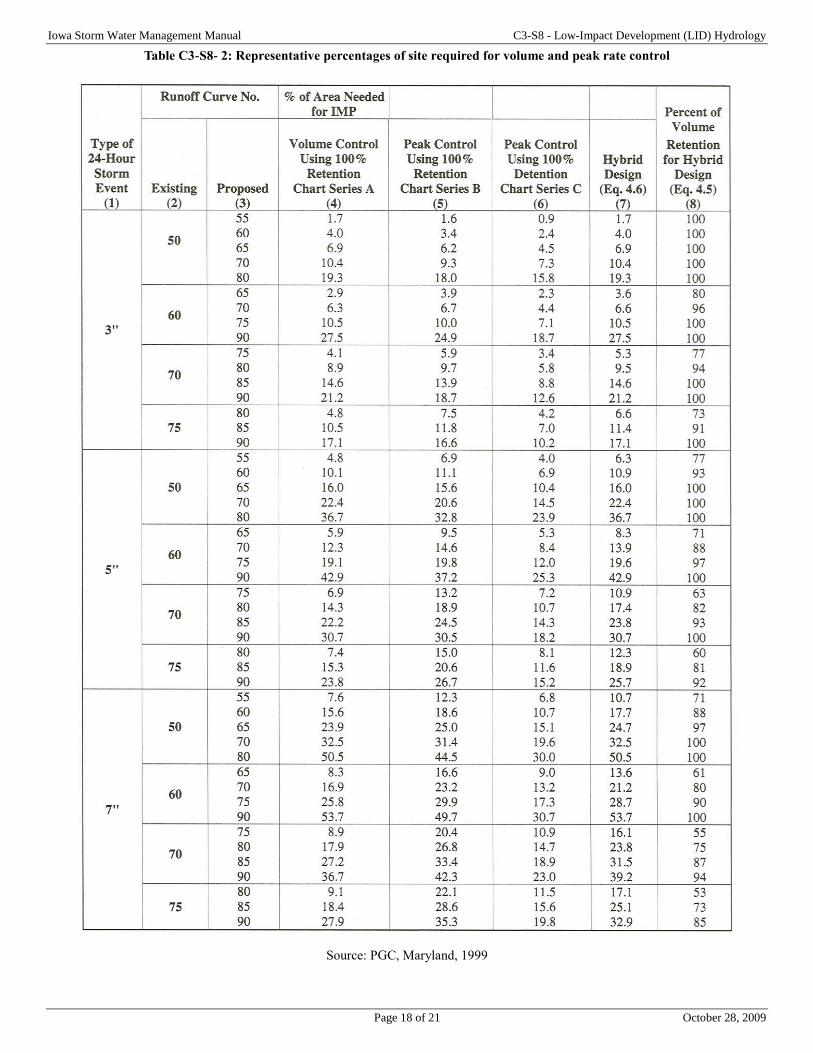
Iowa Storm Water Management Manual C3-S8 - Low-Impact Development (LID) Hydrology
Page 18 of 21 October 28, 2009
Table C3-S8- 2: Representative percentages of site required for volume and peak rate control
Source: PGC, Maryland, 1999
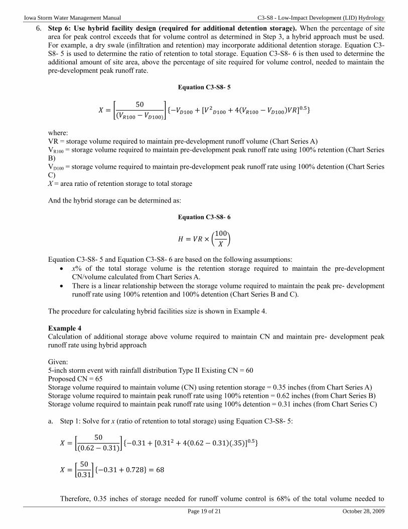
Iowa Storm Water Management Manual C3-S8 - Low-Impact Development (LID) Hydrology
Page 19 of 21 October 28, 2009
6. Step 6: Use hybrid facility design (required for additional detention storage). When the percentage of site
area for peak control exceeds that for volume control as determined in Step 3, a hybrid approach must be used.
For example, a dry swale (infiltration and retention) may incorporate additional detention storage. Equation C3-
S8- 5 is used to determine the ratio of retention to total storage. Equation C3-S8- 6 is then used to determine the
additional amount of site area, above the percentage of site required for volume control, needed to maintain the
pre-development peak runoff rate.
Equation C3-S8- 5
𝑋 = [50
(𝑉𝑅100 − 𝑉𝐷100)] {−𝑉𝐷100 + [𝑉2
𝐷100 + 4(𝑉𝑅100 − 𝑉𝐷100)𝑉𝑅]0.5}
where:
VR = storage volume required to maintain pre-development runoff volume (Chart Series A)
VR100 = storage volume required to maintain pre-development peak runoff rate using 100% retention (Chart Series
B)
VD100 = storage volume required to maintain pre-development peak runoff rate using 100% detention (Chart Series
C)
X = area ratio of retention storage to total storage
And the hybrid storage can be determined as:
Equation C3-S8- 6
𝐻 = 𝑉𝑅 × (100
𝑋)
Equation C3-S8- 5 and Equation C3-S8- 6 are based on the following assumptions:
x% of the total storage volume is the retention storage required to maintain the pre-development
CN/volume calculated from Chart Series A.
There is a linear relationship between the storage volume required to maintain the peak pre- development
runoff rate using 100% retention and 100% detention (Chart Series B and C).
The procedure for calculating hybrid facilities size is shown in Example 4.
Example 4
Calculation of additional storage above volume required to maintain CN and maintain pre- development peak
runoff rate using hybrid approach
Given:
5-inch storm event with rainfall distribution Type II Existing CN = 60
Proposed CN = 65
Storage volume required to maintain volume (CN) using retention storage = 0.35 inches (from Chart Series A)
Storage volume required to maintain peak runoff rate using 100% retention = 0.62 inches (from Chart Series B)
Storage volume required to maintain peak runoff rate using 100% detention = 0.31 inches (from Chart Series C)
a. Step 1: Solve for x (ratio of retention to total storage) using Equation C3-S8- 5:
𝑋 = [50
(0.62 − 0.31)] {−0.31 + [0.312 + 4(0.62 − 0.31)(.35)]0.5}
𝑋 = [50
0.31] {−0.31 + 0.728} = 68
Therefore, 0.35 inches of storage needed for runoff volume control is 68% of the total volume needed to
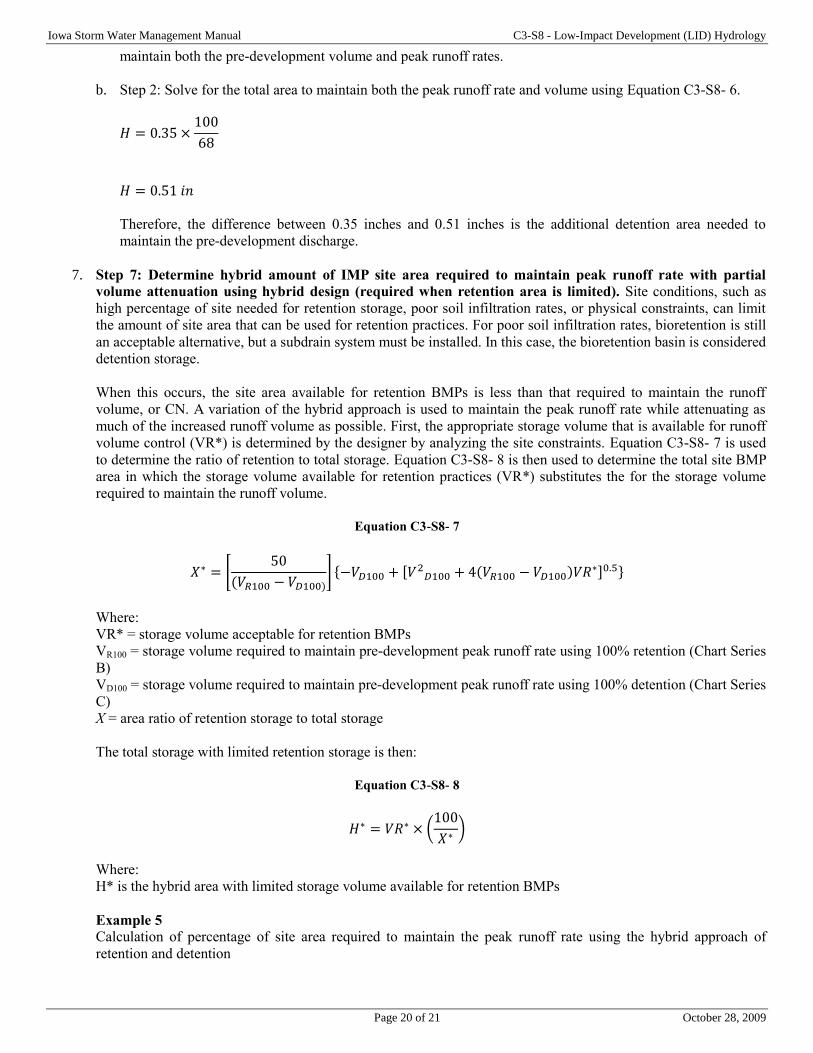
Iowa Storm Water Management Manual C3-S8 - Low-Impact Development (LID) Hydrology
Page 20 of 21 October 28, 2009
maintain both the pre-development volume and peak runoff rates.
b. Step 2: Solve for the total area to maintain both the peak runoff rate and volume using Equation C3-S8- 6.
𝐻 = 0.35 ×100
68
𝐻 = 0.51 𝑖𝑛
Therefore, the difference between 0.35 inches and 0.51 inches is the additional detention area needed to
maintain the pre-development discharge.
7. Step 7: Determine hybrid amount of IMP site area required to maintain peak runoff rate with partial
volume attenuation using hybrid design (required when retention area is limited). Site conditions, such as
high percentage of site needed for retention storage, poor soil infiltration rates, or physical constraints, can limit
the amount of site area that can be used for retention practices. For poor soil infiltration rates, bioretention is still
an acceptable alternative, but a subdrain system must be installed. In this case, the bioretention basin is considered
detention storage.
When this occurs, the site area available for retention BMPs is less than that required to maintain the runoff
volume, or CN. A variation of the hybrid approach is used to maintain the peak runoff rate while attenuating as
much of the increased runoff volume as possible. First, the appropriate storage volume that is available for runoff
volume control (VR*) is determined by the designer by analyzing the site constraints. Equation C3-S8- 7 is used
to determine the ratio of retention to total storage. Equation C3-S8- 8 is then used to determine the total site BMP
area in which the storage volume available for retention practices (VR*) substitutes the for the storage volume
required to maintain the runoff volume.
Equation C3-S8- 7
𝑋∗ = [50
(𝑉𝑅100 − 𝑉𝐷100)] {−𝑉𝐷100 + [𝑉2
𝐷100 + 4(𝑉𝑅100 − 𝑉𝐷100)𝑉𝑅∗]0.5}
Where:
VR* = storage volume acceptable for retention BMPs
VR100 = storage volume required to maintain pre-development peak runoff rate using 100% retention (Chart Series
B)
VD100 = storage volume required to maintain pre-development peak runoff rate using 100% detention (Chart Series
C)
X = area ratio of retention storage to total storage
The total storage with limited retention storage is then:
Equation C3-S8- 8
𝐻∗ = 𝑉𝑅∗ × (100
𝑋∗)
Where:
H* is the hybrid area with limited storage volume available for retention BMPs
Example 5
Calculation of percentage of site area required to maintain the peak runoff rate using the hybrid approach of
retention and detention

Iowa Storm Water Management Manual C3-S8 - Low-Impact Development (LID) Hydrology
Page 21 of 21 October 28, 2009
Given:
5-inch storm event with rainfall distribution Type II
Existing CN = 60
Proposed CN = 65
Storage volume required to maintain volume (CN) = 0.35 in (From Chart Series A)
Storage volume required to maintain peak runoff rate using 100% retention = 0.62 in (from Chart Series B)
Storage volume required to maintain peak runoff rate using 100% detention = 0.31 in (from Chart Series C)
Only half of the required site area is suitable for retention practices, remainder must incorporate detention.
(𝑉𝑅∗ = 0.35 𝑖𝑛 × 0.50 = 0.18 𝑖𝑛).
a. Step 1: Determine appropriate amount of overall BMP area suitable for retention practices. Half of area is
appropriate (given above). Use Equation C3-S8- 7:
𝑋∗ = (50
0.62 − 0.31) × {−0.31 + [0.312 + (4)(. 62 − .31)(0.18)]0.5}
𝑋∗ = (50
. 31) × [−.31 + .565] = 41.1%
Therefore, 0.18 in of storage available for runoff volume control is 41% of the total volume needed for
maintaining the pre-development peak runoff rate.
b. Step 2: Solve for the total area required to maintain the peak runoff rate using Equation C3-S8- 8.
𝐻∗ = 0.18 𝑖𝑛 × (100
41)
𝐻∗ = 0.44 𝑖𝑛
Therefore, a total storage of 0.44 inches is required to maintain the pre-development peak runoff rate but not
the runoff volume. Of the total 0.44-inch storage, 0.18 inches of the storage is used for retention volume.
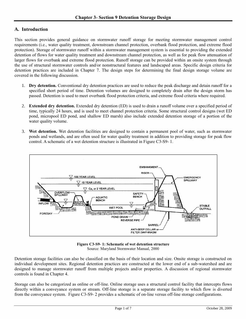
Page 1 of 7 October 28, 2009
Chapter 3- Section 9 Detention Storage Design
A. Introduction
This section provides general guidance on stormwater runoff storage for meeting stormwater management control
requirements (i.e., water quality treatment, downstream channel protection, overbank flood protection, and extreme flood
protection). Storage of stormwater runoff within a stormwater management system is essential to providing the extended
detention of flows for water quality treatment and downstream channel protection, as well as for peak flow attenuation of
larger flows for overbank and extreme flood protection. Runoff storage can be provided within an onsite system through
the use of structural stormwater controls and/or nonstructural features and landscaped areas. Specific design criteria for
detention practices are included in Chapter 7. The design steps for determining the final design storage volume are
covered in the following discussion.
1. Dry detention. Conventional dry detention practices are used to reduce the peak discharge and detain runoff for a
specified short period of time. Detention volumes are designed to completely drain after the design storm has
passed. Detention is used to meet overbank flood protection criteria, and extreme flood criteria where required.
2. Extended dry detention. Extended dry detention (ED) is used to drain a runoff volume over a specified period of
time, typically 24 hours, and is used to meet channel protection criteria. Some structural control designs (wet ED
pond, micropool ED pond, and shallow ED marsh) also include extended detention storage of a portion of the
water quality volume.
3. Wet detention. Wet detention facilities are designed to contain a permanent pool of water, such as stormwater
ponds and wetlands, and are often used for water quality treatment in addition to providing storage for peak flow
control. A schematic of a wet detention structure is illustrated in Figure C3-S9- 1.
Figure C3-S9- 1: Schematic of wet detention structure
Source: Maryland Stormwater Manual, 2000
Detention storage facilities can also be classified on the basis of their location and size. Onsite storage is constructed on
individual development sites. Regional detention practices are constructed at the lower end of a sub-watershed and are
designed to manage stormwater runoff from multiple projects and/or properties. A discussion of regional stormwater
controls is found in Chapter 4.
Storage can also be categorized as online or off-line. Online storage uses a structural control facility that intercepts flows
directly within a conveyance system or stream. Off-line storage is a separate storage facility to which flow is diverted
from the conveyance system. Figure C3-S9- 2 provides a schematic of on-line versus off-line storage configurations.
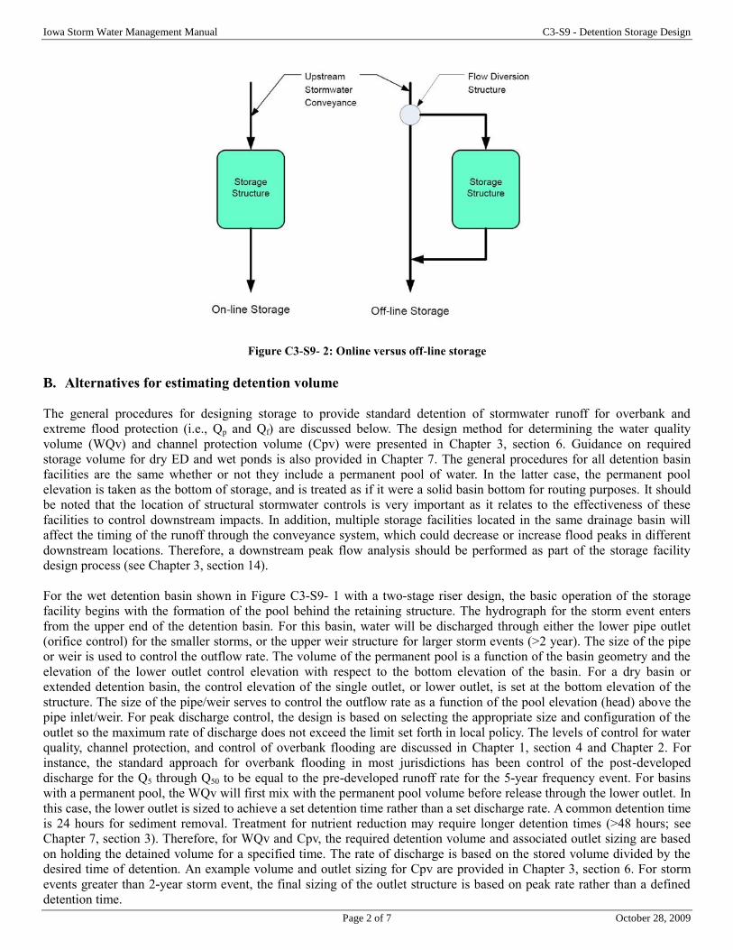
Iowa Storm Water Management Manual C3-S9 - Detention Storage Design
Page 2 of 7 October 28, 2009
Figure C3-S9- 2: Online versus off-line storage
B. Alternatives for estimating detention volume
The general procedures for designing storage to provide standard detention of stormwater runoff for overbank and
extreme flood protection (i.e., Qp and Qf) are discussed below. The design method for determining the water quality
volume (WQv) and channel protection volume (Cpv) were presented in Chapter 3, section 6. Guidance on required
storage volume for dry ED and wet ponds is also provided in Chapter 7. The general procedures for all detention basin
facilities are the same whether or not they include a permanent pool of water. In the latter case, the permanent pool
elevation is taken as the bottom of storage, and is treated as if it were a solid basin bottom for routing purposes. It should
be noted that the location of structural stormwater controls is very important as it relates to the effectiveness of these
facilities to control downstream impacts. In addition, multiple storage facilities located in the same drainage basin will
affect the timing of the runoff through the conveyance system, which could decrease or increase flood peaks in different
downstream locations. Therefore, a downstream peak flow analysis should be performed as part of the storage facility
design process (see Chapter 3, section 14).
For the wet detention basin shown in Figure C3-S9- 1 with a two-stage riser design, the basic operation of the storage
facility begins with the formation of the pool behind the retaining structure. The hydrograph for the storm event enters
from the upper end of the detention basin. For this basin, water will be discharged through either the lower pipe outlet
(orifice control) for the smaller storms, or the upper weir structure for larger storm events (>2 year). The size of the pipe
or weir is used to control the outflow rate. The volume of the permanent pool is a function of the basin geometry and the
elevation of the lower outlet control elevation with respect to the bottom elevation of the basin. For a dry basin or
extended detention basin, the control elevation of the single outlet, or lower outlet, is set at the bottom elevation of the
structure. The size of the pipe/weir serves to control the outflow rate as a function of the pool elevation (head) above the
pipe inlet/weir. For peak discharge control, the design is based on selecting the appropriate size and configuration of the
outlet so the maximum rate of discharge does not exceed the limit set forth in local policy. The levels of control for water
quality, channel protection, and control of overbank flooding are discussed in Chapter 1, section 4 and Chapter 2. For
instance, the standard approach for overbank flooding in most jurisdictions has been control of the post-developed
discharge for the Q5 through Q50 to be equal to the pre-developed runoff rate for the 5-year frequency event. For basins
with a permanent pool, the WQv will first mix with the permanent pool volume before release through the lower outlet. In
this case, the lower outlet is sized to achieve a set detention time rather than a set discharge rate. A common detention time
is 24 hours for sediment removal. Treatment for nutrient reduction may require longer detention times (>48 hours; see
Chapter 7, section 3). Therefore, for WQv and Cpv, the required detention volume and associated outlet sizing are based
on holding the detained volume for a specified time. The rate of discharge is based on the stored volume divided by the
desired time of detention. An example volume and outlet sizing for Cpv are provided in Chapter 3, section 6. For storm
events greater than 2-year storm event, the final sizing of the outlet structure is based on peak rate rather than a defined
detention time.

Iowa Storm Water Management Manual C3-S9 - Detention Storage Design
Page 3 of 7 October 28, 2009
The use of a permanent pool has the advantage of providing improved performance for water quality, aesthetics, and the
provision of wildlife habitat. The disadvantage of systems with permanent pool storage is the increase in total required
storage volume with an increase amount of land (footprint) and perhaps a larger retaining structure. Additional details for
the design of outlet structures are provided in Chapter 3, section 13.
All detention basins are configured with a secondary (emergency) spillway to pass runoff from the 100-year event (Qf),
and to prevent overtopping and subsequent failure of the retaining structure. The elevation of the secondary spillway is
above the elevation of the upper opening on the primary outlet structure, but below the top of the retaining structure. The
sizing of the secondary spillway weir length is established to maintain a minimum freeboard of 1 foot between the basin
water surface elevation at the 100-year event and the top of the retaining structure.
C. Planning and design alternatives
Based on the above discussion, the design of detention structures requires the simultaneous sizing of both the detention
volume characteristics and the outlet riser configuration and size. Planning level (preliminary design) methods will
generally provide an estimate of the required volume of storage to meet a specific stormwater management objective
(Cpv, Qp). Other methods are used to determine the characteristics (dry vs. wet, onsite vs. offsite, etc). The final design is
determined using a method that simultaneously determines the volume of storage and the sizing of the outlet structure.
The simultaneous solution of the volume of storage and outlet sizing is completed using a storage routing procedure.
D. Preliminary detention storage design
A number of methods are available for estimating detention volumes. The ratio of the storage volume to the runoff volume
and the ratio of the pre-development and post-development are the basis for most of these methods. For peak discharge
control objectives, the before-to-after development ratio is called the ratio of outflow/inflow (the peak outflow is the pre-
development peak discharge, and the inflow to the basin equals the post-development peak discharge). Procedures for
preliminary detention calculations are included here to provide a simple method that can be used to estimate storage needs
and also provide a quick check on the results of using different computer programs. Standard storage routing is then used
for actual (final) storage facility calculations and design. Three methods are presented below for determination of
preliminary storage volumes for peak flow reduction:
1. Rational hydrograph method. Based on the difference between the pre- and post-development peak discharges
(ft3/sec) and the pre-development time of concentration, Tc (hr).
2. Wycoff and Singh method. Method for making preliminary hydrologic designs of small flood detention
reservoirs. Developed from a regression of data generated from a more detailed hydrologic model. The time base,
Tb, is measured from the start of runoff to the time when the discharge on the recession limb equals 5% of the
peak discharge rate.
3. The NRCS Urban Hydrology for Small Watersheds (WinTR-55) method. This method has been discussed
earlier (Chapter 3, sections 3, 5, and 6), and is well-documented. The use of WinTR-55 procedures for
determining the runoff volume (Qa), peak discharge (qp), and time of concentration have been discussed
previously. The use of TR-55 for the determination of channel protection volume (Cpv) for extended detention
practices is described in Chapter 3, section 6. The preliminary sizing equation in the worksheet below can be used
for preliminary sizing. The WinTR-55 computer model uses the full TR-20 method of hydrograph generation, and
includes an option for the sizing of detention structures.
4. The low-impact hydrology (LID) method. This method is based on determining the volume of storage required
to reduce the post-development runoff volume to pre-development levels. The LID methodology is summarized in
Chapter 3, section 8. Note that the LID hydrologic method in practice uses complementary practices to increase
the volume of water infiltrated, and reduces the time of concentration by reducing impervious area, lengthening
flow paths across pervious areas, and by using other practices to reduce the volume of direct runoff.
For planning purposes, the assumptions for the Rational method are used to determine an initial estimate for
storage volume. Specifically, a triangular hydrograph with a time to peak equal to Tc and a time base of 2Tc is
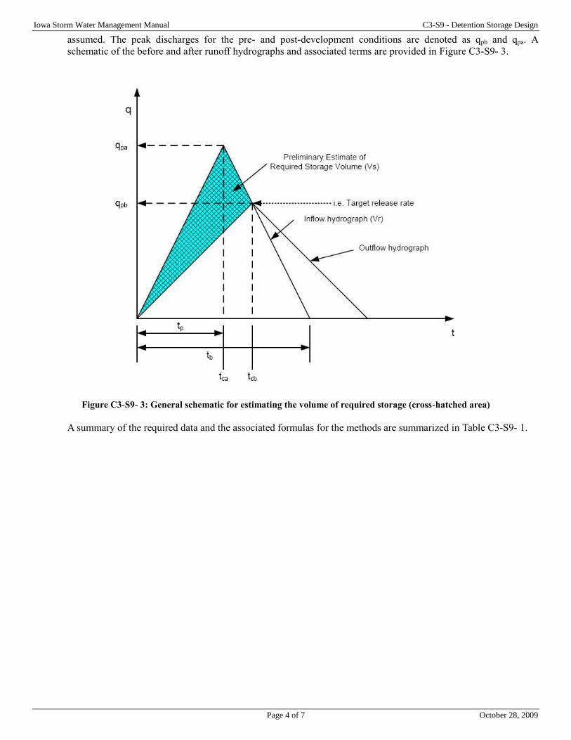
Iowa Storm Water Management Manual C3-S9 - Detention Storage Design
Page 4 of 7 October 28, 2009
assumed. The peak discharges for the pre- and post-development conditions are denoted as qpb and qpa. A
schematic of the before and after runoff hydrographs and associated terms are provided in Figure C3-S9- 3.
Figure C3-S9- 3: General schematic for estimating the volume of required storage (cross-hatched area)
A summary of the required data and the associated formulas for the methods are summarized in Table C3-S9- 1.
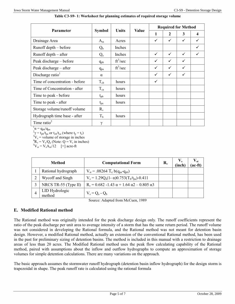
Iowa Storm Water Management Manual C3-S9 - Detention Storage Design
Page 5 of 7 October 28, 2009
Table C3-S9- 1: Worksheet for planning estimates of required storage volume
Parameter Symbol Units Value Required for Method
1 2 3 4
Drainage Area Am Acres
Runoff depth – before Qb Inches
Runoff depth – after Qa Inches
Peak discharge – before qpb ft3/sec
Peak discharge – after qpa ft3/sec
Discharge ratio1 α
Time of concentration - before Tcb hours
Time of Concentration - after Tca hours
Time to peak - before tpb hours
Time to peak - after tpa hours
Storage volume/runoff volume Rv
Hydrograph time base - after Tb hours
Time ratio2 γ
1α = qpb/qpa
2γ = tpb/tpa or tcb/tca (where tp = tc)
3Vs = volume of storage in inches
4Rv = Vs/Qa (Note: Q = Vr in inches)
5Vst = VsAm/12 [=] acre-ft
Method Computational Form Rv Vs
(inch)
Vst
(ac-ft)
1 Rational hydrograph Vst = .08264 Tc b(qpa-qpb)
2 Wycoff and Singh Vs = 1.29Qa(1- α)0.753(Tb/tpa)-0.411
3 NRCS TR-55 (Type II) Rv = 0.682 -1.43 α + 1.64 α2 – 0.805 α3
4 LID Hydrologic
method Vs = Qa - Qb
Source: Adapted from McCuen, 1989
E. Modified Rational method
The Rational method was originally intended for the peak discharge design only. The runoff coefficients represent the
ratio of the peak discharge per unit area to average intensity of a storm that has the same return period. The runoff volume
was not considered in developing the Rational formula, and the Rational method was not meant for detention basin
design. However, a modified Rational method, actually an extension of the conventional Rational method, has been used
in the past for preliminary sizing of detention basins. The method is included in this manual with a restriction to drainage
areas of less than 20 acres. The Modified Rational method uses the peak flow calculating capability of the Rational
method, paired with assumptions about the inflow and outflow hydrographs to compute an approximation of storage
volumes for simple detention calculations. There are many variations on the approach.
The basic approach assumes the stormwater runoff hydrograph (detention basin inflow hydrograph) for the design storm is
trapezoidal in shape. The peak runoff rate is calculated using the rational formula
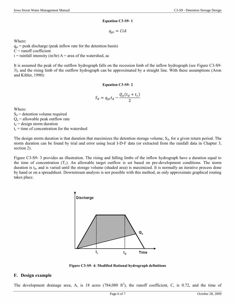
Iowa Storm Water Management Manual C3-S9 - Detention Storage Design
Page 6 of 7 October 28, 2009
Equation C3-S9- 1
𝑞𝑝𝑖 = 𝐶𝑖𝐴
Where:
qpi = peak discharge (peak inflow rate for the detention basin)
C = runoff coefficient
i = rainfall intensity (in/hr) A = area of the watershed, ac
It is assumed the peak of the outflow hydrograph falls on the recession limb of the inflow hydrograph (see Figure C3-S9-
3), and the rising limb of the outflow hydrograph can be approximated by a straight line. With these assumptions (Aron
and Kibler, 1990):
Equation C3-S9- 2
𝑆𝑑 = 𝑞𝑝𝑖𝑡𝑑 −𝑄𝑎(𝑡𝑑 + 𝑡𝑐)
2
Where:
Sd = detention volume required
Qa = allowable peak outflow rate
td = design storm duration
tc = time of concentration for the watershed
The design storm duration is that duration that maximizes the detention storage volume, Sd, for a given return period. The
storm duration can be found by trial and error using local I-D-F data (or extracted from the rainfall data in Chapter 3,
section 2).
Figure C3-S9- 3 provides an illustration. The rising and falling limbs of the inflow hydrograph have a duration equal to
the time of concentration (Tc). An allowable target outflow is set based on pre-development conditions. The storm
duration is td, and is varied until the storage volume (shaded area) is maximized. It is normally an iterative process done
by hand or on a spreadsheet. Downstream analysis is not possible with this method, as only approximate graphical routing
takes place.
Figure C3-S9- 4: Modified Rational hydrograph definitions
F. Design example
The development drainage area, A, is 18 acres (784,080 ft2), the runoff coefficient, C, is 0.72, and the time of
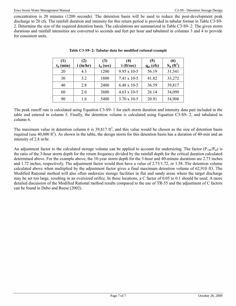
Iowa Storm Water Management Manual C3-S9 - Detention Storage Design
Page 7 of 7 October 28, 2009
concentration is 20 minutes (1200 seconds). The detention basin will be used to reduce the post-development peak
discharge to 20 cfs. The rainfall duration and intensity for this return period is provided in tabular format in Table C3-S9-
2. Determine the size of the required detention basin. The calculations are summarized in Table C3-S9- 2. The given storm
durations and rainfall intensities are converted to seconds and feet per hour and tabulated in columns 3 and 4 to provide
for consistent units.
Table C3-S9- 2: Tabular data for modified rational example
(1)
td (min)
(2)
i (in/hr)
(3)
td (sec)
(4)
i (ft/sec)
(5)
qpi (cfs)
(6)
Sd (ft3)
20 4.3 1200 9.95 x 10⁻⁵ 56.19 31,341
30 3.2 1800 7.41 x 10⁻⁵ 41.82 33,272
40 2.8 2400 6.48 x 10⁻⁵ 36.59 39,817
60 2.0 3600 4.63 x 10⁻⁵ 26.14 34,090
90 1.6 5400 3.70 x 10⁻⁵ 20.91 34,908
The peak runoff rate is calculated using Equation C3-S9- 1 for each storm duration and intensity data pair included in the
table and entered in column 5. Finally, the detention volume is calculated using Equation C3-S9- 2, and tabulated in
column 6.
The maximum value in detention column 6 is 39,817 ft3, and this value would be chosen as the size of detention basin
required (use 40,000 ft3). As shown in the table, the design storm for this detention basin has a duration of 40-min and an
intensity of 2.8 in/hr.
An adjustment factor to the calculated storage volume can be applied to account for undersizing. The factor (P180/Ptd) is
the ratio of the 3-hour storm depth for the return frequency divided by the rainfall depth for the critical duration calculated
determined above. For the example above, the 10-year storm depth for the 3-hour and 40-minute durations are 2.73 inches
and 1.72 inches, respectively. The adjustment factor would then have a value of 2.73/1.72, or 1.58. The detention volume
calculated above when multiplied by the adjustment factor gives a final maximum detention volume of 62,910 ft3. The
Modified Rational method will also often undersize storage facilities in flat and sandy areas where the target discharge
may be set too large, resulting in an oversized orifice. In these locations, a C factor of 0.05 to 0.1 should be used. A more
detailed discussion of the Modified Rational method results compared to the use of TR-55 and the adjustment of C factors
can be found in Debo and Reese (2002).
Page 1 of 14 October 28, 2009
Chapter 3- Section 10 Channel and Storage (Reservoir) Routing
A. Introduction
Flood routing is the process of calculating the passage of the runoff hydrograph through a conveyance system. If the
system is a channel, the flood routing is called a channel (stream flow) routing. If the system is a reservoir, the terms
storage routing or reservoir routing are applied.
B. Channel routing
Channel flow elements in urban watersheds include gutters, ditches, swales, and sewers. During a rainfall event, unsteady
flow will occur in these conveyance elements. Channel routing is the term applied to methods of accounting for the effects
of channel storage on the runoff hydrograph as the hydrograph moves through the channel reach. The input and output
functions for the channel routing procedure consists of the runoff hydrographs for upstream and downstream sections of a
channel. These two functions are related by a channel routing procedure used to translate and attenuate the upstream
runoff hydrograph into a downstream hydrograph. The routing procedure has two components – the routing method and
the physical channel characteristics of the stream reach. The channel characteristics (slope, roughness, cross section,
vegetation, etc.) can generally be quantified from visual and engineering surveys so the routing method becomes the
primary design tool. Where existing measured hydrograph data exists for a channel reach, the coefficients for the routing
function can be determined. However, for most design situations, the measured hydrograph data is not available. In this
case, the upstream hydrograph is synthesized using methods discussed in Chapter 3, section 7, and the resulting
downstream runoff hydrograph is computed. Two general approaches are used for solving the unsteady flow problem in
channels – hydrologic and hydraulic. The hydrologic approach is based on the storage concept while the hydraulic
approach uses principles of mass and momentum conservation. The Muskingum method is used for the hydrologic
approach, while the kinematic wave method is used for the hydraulic transformation. The Muskingum method and the
related Muskingum-Cunge modification are presented in this manual as the preferred methods for channel routing.
1. Muskingum method. For the Muskingum routing, the hydrologic storage equation for a channel reach is:
Equation C3-S10- 1
𝐼 − 𝑂 =𝑑𝑆
𝑑𝑡~
∆𝑆
∆𝑡
Where:
I and O are the inflow and outflow rates respectively during the incremental time, ∆t,
S is volume of water in storage in the channel reach
For the hydrographs shown in Figure C3-S10- 1, the continuity equation can be expressed in terms of the inflow
(upstream) and outflow (downstream) at two times, t1 and t2, separated by the time increment ∆t = t2-t1.
The numerical form of the routing equation is expressed in Equation C3-S10- 2:
Equation C3-S10- 2
𝑆2 − 𝑆1
∆𝑡= 1
2⁄ (𝐼1 + 𝐼2) − 12⁄ (𝑂1 + 𝑂2)
Assuming the inflow hydrograph is known for all t, and the initial outflow and storage, O1 and S1 are known at
time t, then Equation C3-S10- 2 has two unknowns. To use the routing equation, a second relationship is needed.
The inflow storage is related to the inflow rate and the outflow storage to the outflow rate, as follows:
Equation C3-S10- 2a
𝑆𝑖 = 𝐾𝐼𝑛
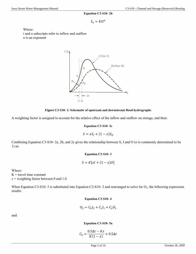
Iowa Storm Water Management Manual C3-S10 - Channel and Storage (Reservoir) Routing
Page 2 of 14 October 28, 2009
Equation C3-S10- 2b
𝑆𝑜 = 𝐾𝑂𝑛
Where:
i and o subscripts refer to inflow and outflow
n is an exponent
Figure C3-S10- 1: Schematic of upstream and downstream flood hydrographs
A weighting factor is assigned to account for the relative effect of the inflow and outflow on storage, and then:
Equation C3-S10- 2c
𝑆 = 𝑥𝑆𝐼 + (1 − 𝑥)𝑆𝑂
Combining Equation C3-S10- 2a, 2b, and 2c gives the relationship between S, I and O (n is commonly determined to be
1) as:
Equation C3-S10- 3
𝑆 = 𝐾[𝑥𝐼 + (1 − 𝑥)𝑂]
Where:
K = travel time constant
x = weighting factor between 0 and 1.0
When Equation C3-S10- 3 is substituted into Equation C3-S10- 2 and rearranged to solve for O2, the following expression
results:
Equation C3-S10- 4
𝑂2 = 𝐶0𝐼2 + 𝐶1𝐼1 + 𝐶2𝑂1
and:
Equation C3-S10- 5a
𝐶0 =0.5∆𝑡 − 𝐾𝑥
𝐾(1 − 𝑥)+ 0.5∆𝑡
Iowa Storm Water Management Manual C3-S10 - Channel and Storage (Reservoir) Routing
Page 3 of 14 October 28, 2009
Equation C3-S10- 5b
𝐶1 =0.5∆𝑡 − 𝐾𝑥
𝐾(1 − 𝑥)+ 0.5∆𝑡
Equation C3-S10- 5c
𝐶2 =[𝐾(1 − 𝑥) − 0.5∆𝑡]
𝐾(1 − 𝑥)+ 0.5∆𝑡
Equation C3-S10- 4 is the Muskingum routing equation and C0, C1 and C2 are the routing weighting factors.
𝐶0 + 𝐶1 + 𝐶2 = 1.0
Given an inflow hydrograph, an initial flow condition, a chosen time interval (tp/∆t ≥5), and routing parameters K and x,
the routing coefficients can be calculated in Equation C3-S10- 5a through 5c and the outflow hydrograph from Equation
C3-S10- 4. The routing parameters K and x are related to flow and channel characteristics, K being interpreted as the
travel time of the flood wave from upstream to downstream end of the channel reach; K is therefore a function of channel
length and flood wave speed. The parameter x accounts for the storage portion of the routing – for a given flood event,
there is a value of x for which the storage in the calculated outflow hydrograph matches the measured outflow
hydrograph. In the Muskingum method, x is used as a weighting factor and restricted to a range of values of 0.0 to 0.5. At
x > 0.5, the outflow hydrograph becomes greater than the inflow hydrograph (hydrograph amplification). At K = ∆t and x
= 0.5, the outflow hydrograph retains the same shape as the inflow and is just translated downstream a time equal to K.
For x= 0, the Muskingum routing reduced to a linear reservoir routing.
The K and x parameters in the Muskingum method are determined by calibration using streamflow records. The detailed
procedure for the calibration is discussed in McCuen (1989).
2. Muskingum-Cunge method. An alternative, but related method to the Muskingum procedure, is the
Muskingum-Cunge method, which uses a kinematic wave (conservation of mass/momentum) approach. The main
advantage of the Muskingum-Cunge method is that the routing coefficients are evaluated from physical channel
characteristics and can be determined without existing flood hydrograph data. In the method, for a channel
section, it is assumed that:
Equation C3-S10- 6
𝑄 = 𝑒𝐴𝑚
Where:
Q = discharge, cfs
A = flow area, ft2
e, m = constant parameters
The relationship in Equation C3-S10- 6 can be obtained from a stream channel rating curve. A rating curve can be
prepared using the Manning formula. For certain shapes of channels (i.e. triangular, trapezoidal, parabolic), the
Manning formula will yield constant values for e and m. For other x-sectional shapes, e and m will change with
discharge, and average values will need to be used. To apply the Muskingum-Cunge model, first choose a
reference flow condition represented by:
Q0 = reference discharge, cfs
T0 = top width of the flow at Q0, ft
V0 = cross-sectional average velocity at Q0, fps
A0 = flow area at Q0, ft2
The reference discharge can be chosen as the base flow rate, the peak flow of the inflow hydrograph, or the
average inflow rate. Form these reference conditions and the channel characteristics, the Muskingum constants K
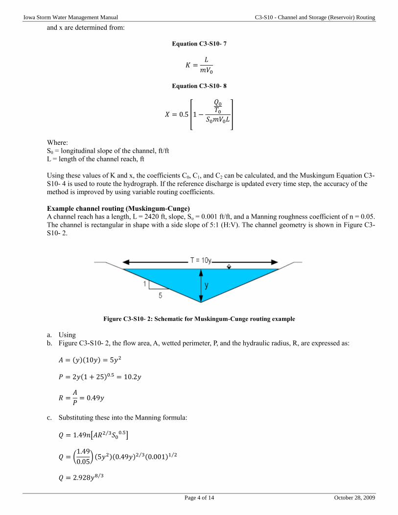
Iowa Storm Water Management Manual C3-S10 - Channel and Storage (Reservoir) Routing
Page 4 of 14 October 28, 2009
and x are determined from:
Equation C3-S10- 7
𝐾 =𝐿
𝑚𝑉0
Equation C3-S10- 8
𝑋 = 0.5 [1 −
𝑄0𝑇0
𝑆0𝑚𝑉0𝐿]
Where:
S0 = longitudinal slope of the channel, ft/ft
L = length of the channel reach, ft
Using these values of K and x, the coefficients C0, C1, and C2 can be calculated, and the Muskingum Equation C3-
S10- 4 is used to route the hydrograph. If the reference discharge is updated every time step, the accuracy of the
method is improved by using variable routing coefficients.
Example channel routing (Muskingum-Cunge)
A channel reach has a length, L = 2420 ft, slope, So = 0.001 ft/ft, and a Manning roughness coefficient of n = 0.05.
The channel is rectangular in shape with a side slope of 5:1 (H:V). The channel geometry is shown in Figure C3-
S10- 2.
Figure C3-S10- 2: Schematic for Muskingum-Cunge routing example
a. Using
b. Figure C3-S10- 2, the flow area, A, wetted perimeter, P, and the hydraulic radius, R, are expressed as:
𝐴 = (𝑦)(10𝑦) = 5𝑦2
𝑃 = 2𝑦(1 + 25)0.5 = 10.2𝑦
𝑅 =𝐴
𝑃= 0.49𝑦
c. Substituting these into the Manning formula:
𝑄 = 1.49𝑛[𝐴𝑅2 3⁄ 𝑆00.5]
𝑄 = (1.49
0.05) (5𝑦2)(0.49𝑦)2 3⁄ (0.001)1 2⁄
𝑄 = 2.928𝑦8 3⁄
Iowa Storm Water Management Manual C3-S10 - Channel and Storage (Reservoir) Routing
Page 5 of 14 October 28, 2009
and since 𝐴 = 5𝑦2:
𝑄 = 0.343𝐴4 3⁄
Therefore, using Equation C3-S10- 6, 𝑒 = 0.343𝑓𝑡1 3⁄ /𝑠𝑒𝑐, and m = 4/3.
d. An inflow hydrograph for a small watershed is tabulated in Table C3-S10- 1. Complete the routing through
the channel described above. A time increment of ∆t = 0.5 hours and a reference discharge of 10 cfs (base
flow) will be used.
e. To begin the solution, first determine T0 and V0. Using the reference discharge of Q = 10 cfs:
𝐴0 = (10
0.343)
3 4⁄
= 12.55𝑓𝑡2
𝑦0 = (12.55𝑓𝑡2
5)
0.5
= 1.58𝑓𝑡
𝑇0 = (10)(1.58) = 15.8𝑓𝑡
𝑉0 =10𝑐𝑓𝑠
12.55𝑓𝑡2= 0.797𝑓𝑝𝑠
From Equation C3-S10- 7 and Equation C3-S10- 8:
𝐾 =2420𝑓𝑡
[(4 3⁄ )(0.797𝑓𝑝𝑠)]= 2277𝑠𝑒𝑐 = 0.632ℎ𝑟
𝑋 = 0.5 {1 − [
10𝑐𝑓𝑠15.8𝑓𝑡
(0.001)(4 3⁄ )(0.797𝑓𝑝𝑠)(242𝑓𝑡)]} = 0.377
f. Next compute C0, C1, and C3 from Equation C3-S10- 5a through 5c:
𝐶0 = 0.0182
𝐶1 = 0.7585
𝐶2 = 0.2233
The routing is completed using the routing Equation C3-S10- 4, and the results are listed in Table C3-S10- 1.
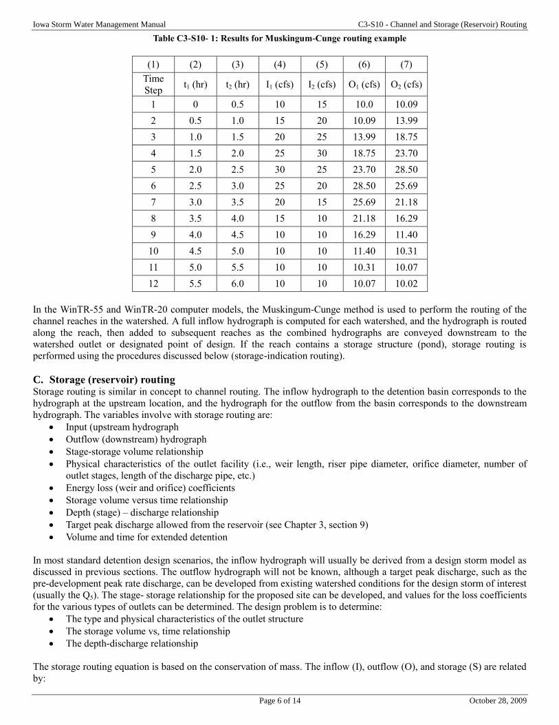
Iowa Storm Water Management Manual C3-S10 - Channel and Storage (Reservoir) Routing
Page 6 of 14 October 28, 2009
Table C3-S10- 1: Results for Muskingum-Cunge routing example
(1) (2) (3) (4) (5) (6) (7)
Time
Step t1 (hr) t2 (hr) I1 (cfs) I2 (cfs) O1 (cfs) O2 (cfs)
1 0 0.5 10 15 10.0 10.09
2 0.5 1.0 15 20 10.09 13.99
3 1.0 1.5 20 25 13.99 18.75
4 1.5 2.0 25 30 18.75 23.70
5 2.0 2.5 30 25 23.70 28.50
6 2.5 3.0 25 20 28.50 25.69
7 3.0 3.5 20 15 25.69 21.18
8 3.5 4.0 15 10 21.18 16.29
9 4.0 4.5 10 10 16.29 11.40
10 4.5 5.0 10 10 11.40 10.31
11 5.0 5.5 10 10 10.31 10.07
12 5.5 6.0 10 10 10.07 10.02
In the WinTR-55 and WinTR-20 computer models, the Muskingum-Cunge method is used to perform the routing of the
channel reaches in the watershed. A full inflow hydrograph is computed for each watershed, and the hydrograph is routed
along the reach, then added to subsequent reaches as the combined hydrographs are conveyed downstream to the
watershed outlet or designated point of design. If the reach contains a storage structure (pond), storage routing is
performed using the procedures discussed below (storage-indication routing).
C. Storage (reservoir) routing Storage routing is similar in concept to channel routing. The inflow hydrograph to the detention basin corresponds to the
hydrograph at the upstream location, and the hydrograph for the outflow from the basin corresponds to the downstream
hydrograph. The variables involve with storage routing are:
Input (upstream hydrograph
Outflow (downstream) hydrograph
Stage-storage volume relationship
Physical characteristics of the outlet facility (i.e., weir length, riser pipe diameter, orifice diameter, number of
outlet stages, length of the discharge pipe, etc.)
Energy loss (weir and orifice) coefficients
Storage volume versus time relationship
Depth (stage) – discharge relationship
Target peak discharge allowed from the reservoir (see Chapter 3, section 9)
Volume and time for extended detention
In most standard detention design scenarios, the inflow hydrograph will usually be derived from a design storm model as
discussed in previous sections. The outflow hydrograph will not be known, although a target peak discharge, such as the
pre-development peak rate discharge, can be developed from existing watershed conditions for the design storm of interest
(usually the Q5). The stage- storage relationship for the proposed site can be developed, and values for the loss coefficients
for the various types of outlets can be determined. The design problem is to determine:
The type and physical characteristics of the outlet structure
The storage volume vs, time relationship
The depth-discharge relationship
The storage routing equation is based on the conservation of mass. The inflow (I), outflow (O), and storage (S) are related
by:
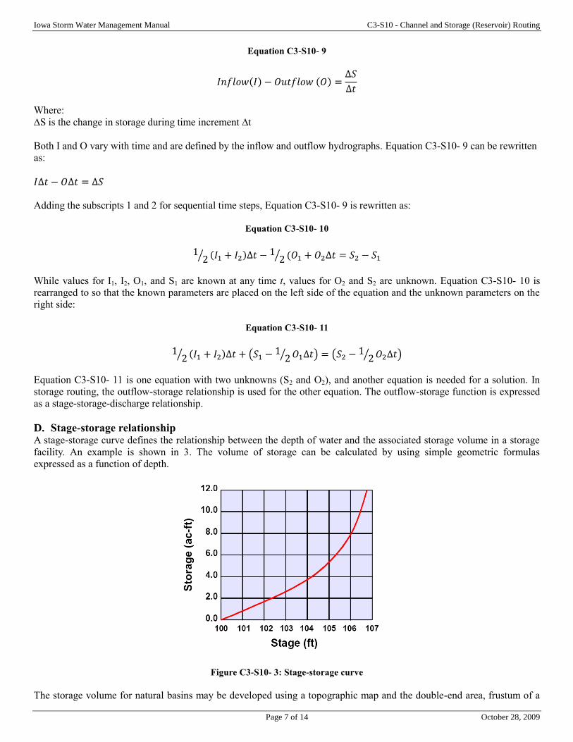
Iowa Storm Water Management Manual C3-S10 - Channel and Storage (Reservoir) Routing
Page 7 of 14 October 28, 2009
Equation C3-S10- 9
𝐼𝑛𝑓𝑙𝑜𝑤(𝐼) − 𝑂𝑢𝑡𝑓𝑙𝑜𝑤 (𝑂) =∆𝑆
∆𝑡
Where:
∆S is the change in storage during time increment ∆t
Both I and O vary with time and are defined by the inflow and outflow hydrographs. Equation C3-S10- 9 can be rewritten
as:
𝐼∆𝑡 − 𝑂∆𝑡 = ∆𝑆
Adding the subscripts 1 and 2 for sequential time steps, Equation C3-S10- 9 is rewritten as:
Equation C3-S10- 10
12⁄ (𝐼1 + 𝐼2)∆𝑡 − 1
2⁄ (𝑂1 + 𝑂2∆𝑡 = 𝑆2 − 𝑆1
While values for I1, I2, O1, and S1 are known at any time t, values for O2 and S2 are unknown. Equation C3-S10- 10 is
rearranged to so that the known parameters are placed on the left side of the equation and the unknown parameters on the
right side:
Equation C3-S10- 11
12⁄ (𝐼1 + 𝐼2)∆𝑡 + (𝑆1 − 1
2⁄ 𝑂1∆𝑡) = (𝑆2 − 12⁄ 𝑂2∆𝑡)
Equation C3-S10- 11 is one equation with two unknowns (S2 and O2), and another equation is needed for a solution. In
storage routing, the outflow-storage relationship is used for the other equation. The outflow-storage function is expressed
as a stage-storage-discharge relationship.
D. Stage-storage relationship A stage-storage curve defines the relationship between the depth of water and the associated storage volume in a storage
facility. An example is shown in 3. The volume of storage can be calculated by using simple geometric formulas
expressed as a function of depth.
Figure C3-S10- 3: Stage-storage curve
The storage volume for natural basins may be developed using a topographic map and the double-end area, frustum of a
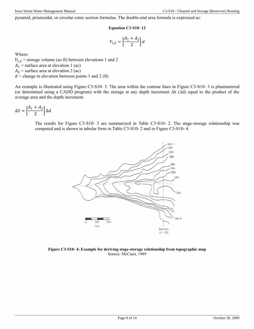
Iowa Storm Water Management Manual C3-S10 - Channel and Storage (Reservoir) Routing
Page 8 of 14 October 28, 2009
pyramid, prismoidal, or circular conic section formulas. The double-end area formula is expressed as:
Equation C3-S10- 12
𝑉1,2 = [𝐴1 + 𝐴2
2] 𝑑
Where:
𝑉1,2 = storage volume (ac-ft) between elevations 1 and 2
𝐴1 = surface area at elevation 1 (ac)
𝐴2 = surface area at elevation 2 (ac)
𝑑 = change in elevation between points 1 and 2 (ft)
An example is illustrated using Figure C3-S10- 3. The area within the contour lines in Figure C3-S10- 3 is planimetered
(or determined using a CADD program) with the storage at any depth increment ∆h (∆d) equal to the product of the
average area and the depth increment.
∆𝑆 = [𝐴1 + 𝐴2
2] ∆𝑑
The results for Figure C3-S10- 3 are summarized in Table C3-S10- 2. The stage-storage relationship was
computed and is shown in tabular form in Table C3-S10- 2 and in Figure C3-S10- 4.
Figure C3-S10- 4: Example for deriving stage-storage relationship from topographic map
Source: McCuen, 1989
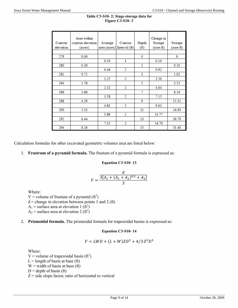
Iowa Storm Water Management Manual C3-S10 - Channel and Storage (Reservoir) Routing
Page 9 of 14 October 28, 2009
Table C3-S10- 2: Stage-storage data for
Figure C3-S10- 3
Calculation formulas for other excavated geometric volumes area are listed below:
1. Frustrum of a pyramid formula. The frustum of a pyramid formula is expressed as:
Equation C3-S10- 13
𝑉 =
𝑑3[𝐴1 + (𝐴1 + 𝐴2)0.5 + 𝐴2]
3
Where:
V = volume of frustum of a pyramid (ft3)
d = change in elevation between points 1 and 2 (ft)
A1 = surface area at elevation 1 (ft2)
A2 = surface area at elevation 2 (ft2)
2. Prismoidal formula. The prismoidal formula for trapezoidal basins is expressed as:
Equation C3-S10- 14
𝑉 = 𝐿𝑊𝐷 + (𝐿 + 𝑊)𝑍𝐷2 + 4 3⁄ 𝑍2𝐷3
Where:
V = volume of trapezoidal basin (ft3)
L = length of basin at base (ft)
W = width of basin at base (ft)
D = depth of basin (ft)
Z = side slope factor, ratio of horizontal to vertical
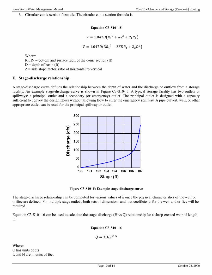
Iowa Storm Water Management Manual C3-S10 - Channel and Storage (Reservoir) Routing
Page 10 of 14 October 28, 2009
3. Circular conic section formula. The circular conic section formula is:
Equation C3-S10- 15
𝑉 = 1.047𝐷(𝑅12 + 𝑅2
2 + 𝑅1𝑅2)
𝑉 = 1.047𝐷(3𝑅12 + 3𝑍𝐷𝑅1 + 𝑍2𝐷2)
Where:
R1, R2 = bottom and surface radii of the conic section (ft)
D = depth of basin (ft)
Z = side slope factor, ratio of horizontal to vertical
E. Stage-discharge relationship
A stage-discharge curve defines the relationship between the depth of water and the discharge or outflow from a storage
facility. An example stage-discharge curve is shown in Figure C3-S10- 5. A typical storage facility has two outlets or
spillways: a principal outlet and a secondary (or emergency) outlet. The principal outlet is designed with a capacity
sufficient to convey the design flows without allowing flow to enter the emergency spillway. A pipe culvert, weir, or other
appropriate outlet can be used for the principal spillway or outlet.
Figure C3-S10- 5: Example stage-discharge curve
The stage-discharge relationship can be computed for various values of h once the physical characteristics of the weir or
orifice are defined. For multiple stage outlets, both sets of dimensions and loss coefficients for the weir and orifice will be
required.
Equation C3-S10- 16 can be used to calculate the stage-discharge (H vs Q) relationship for a sharp-crested weir of length
L.
Equation C3-S10- 16
𝑄 = 3.3𝐿𝐻1.5
Where:
Q has units of cfs
L and H are in units of feet
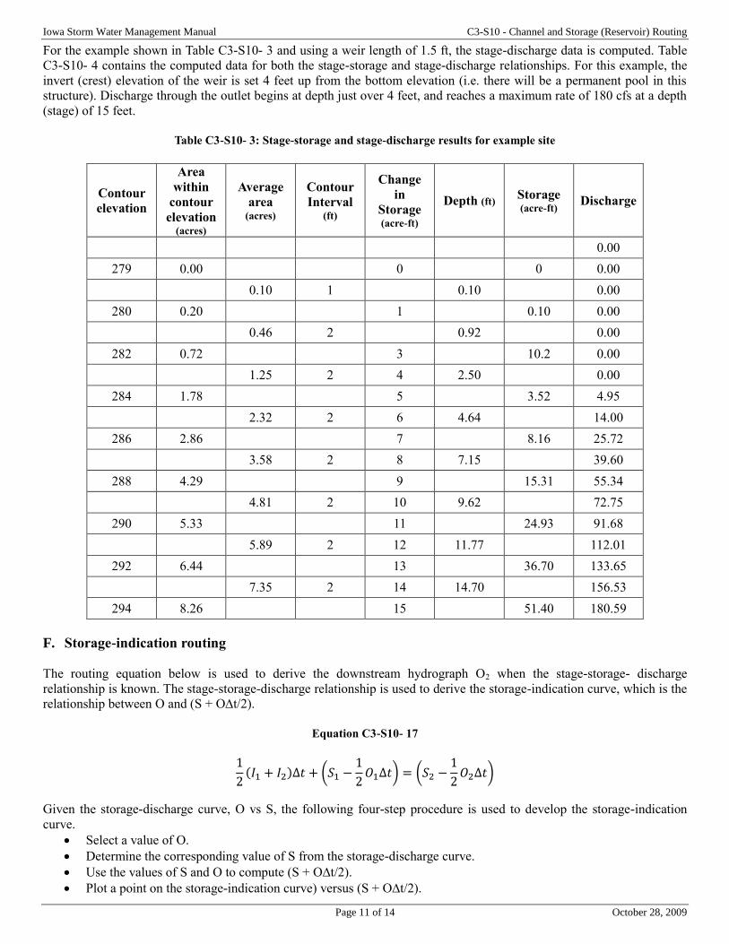
Iowa Storm Water Management Manual C3-S10 - Channel and Storage (Reservoir) Routing
Page 11 of 14 October 28, 2009
For the example shown in Table C3-S10- 3 and using a weir length of 1.5 ft, the stage-discharge data is computed. Table
C3-S10- 4 contains the computed data for both the stage-storage and stage-discharge relationships. For this example, the
invert (crest) elevation of the weir is set 4 feet up from the bottom elevation (i.e. there will be a permanent pool in this
structure). Discharge through the outlet begins at depth just over 4 feet, and reaches a maximum rate of 180 cfs at a depth
(stage) of 15 feet.
Table C3-S10- 3: Stage-storage and stage-discharge results for example site
Contour
elevation
Area
within
contour
elevation (acres)
Average
area (acres)
Contour
Interval (ft)
Change
in
Storage (acre-ft)
Depth (ft) Storage (acre-ft)
Discharge
0.00
279 0.00 0 0 0.00
0.10 1 0.10 0.00
280 0.20 1 0.10 0.00
0.46 2 0.92 0.00
282 0.72 3 10.2 0.00
1.25 2 4 2.50 0.00
284 1.78 5 3.52 4.95
2.32 2 6 4.64 14.00
286 2.86 7 8.16 25.72
3.58 2 8 7.15 39.60
288 4.29 9 15.31 55.34
4.81 2 10 9.62 72.75
290 5.33 11 24.93 91.68
5.89 2 12 11.77 112.01
292 6.44 13 36.70 133.65
7.35 2 14 14.70 156.53
294 8.26 15 51.40 180.59
F. Storage-indication routing
The routing equation below is used to derive the downstream hydrograph O2 when the stage-storage- discharge
relationship is known. The stage-storage-discharge relationship is used to derive the storage-indication curve, which is the
relationship between O and (S + O∆t/2).
Equation C3-S10- 17
1
2(𝐼1 + 𝐼2)∆𝑡 + (𝑆1 −
1
2𝑂1∆𝑡) = (𝑆2 −
1
2𝑂2∆𝑡)
Given the storage-discharge curve, O vs S, the following four-step procedure is used to develop the storage-indication
curve.
Select a value of O.
Determine the corresponding value of S from the storage-discharge curve.
Use the values of S and O to compute (S + O∆t/2).
Plot a point on the storage-indication curve) versus (S + O∆t/2).

Iowa Storm Water Management Manual C3-S10 - Channel and Storage (Reservoir) Routing
Page 12 of 14 October 28, 2009
The steps are repeated for a sufficient number of values for O to define the storage-indication curve.
The objective of the storage-indication method is to derive the outflow hydrograph. Five data sources are required as
follows:
Storage-discharge relationship (based on site geometry)
Storage-indication curve
Inflow hydrograph (from hydrograph synthesis or computer output)
Initial values of the storage and outflow rate.
Routing increment (∆t ≥ tp/5); tp = 2/3 Tc
The outflow hydrograph is the main output of interest for most design cases. However, the storage function, S vs. t, can
also be determined from the storage-indication method. As a check on the final design, one may want to know the storage
(and hence water surface elevation) as a function of time. The following five steps can be sued to derive the outflow
hydrograph with the storage-time function as a by-product.
Determine the average inflow: 0.5∆t(I1 + I2)
Compute S1 – 1/2O1∆t
Using Equation C3-S10- 17 and the values from Steps 1 and 2, compute S2 + 1/2O2∆t
Using the value computed in Step 3, determine O2 from the storage-indication curve
Use O2 with the storage-discharge relationship to obtain S2
The five steps are repeated for the next time-increment using I2, O2, and S2 as the new values of I1, O1, and S1,
respectively. The process is solved iteratively until the entire outflow hydrograph is compiled. Once the stage-storage-
discharge relationships and the storage-indication curve data are determined and plotted, a mathematical expression can be
developed for each and used in a spreadsheet computation to speed the process.
The procedure is an iterative solution and does involve a number of calculation steps. The procedure may also need to be
repeated over several trial calculations should the outlet configuration need to be modified to meet a peak discharge
limitation. WinTR-55 and WinTR-20 contain the storage- indication routing procedure to assist with the design of
detention structures. The advantage of the computer models is the speed at which the designed can check several trial
sizes of outlet structures to achieve the correct level of control.
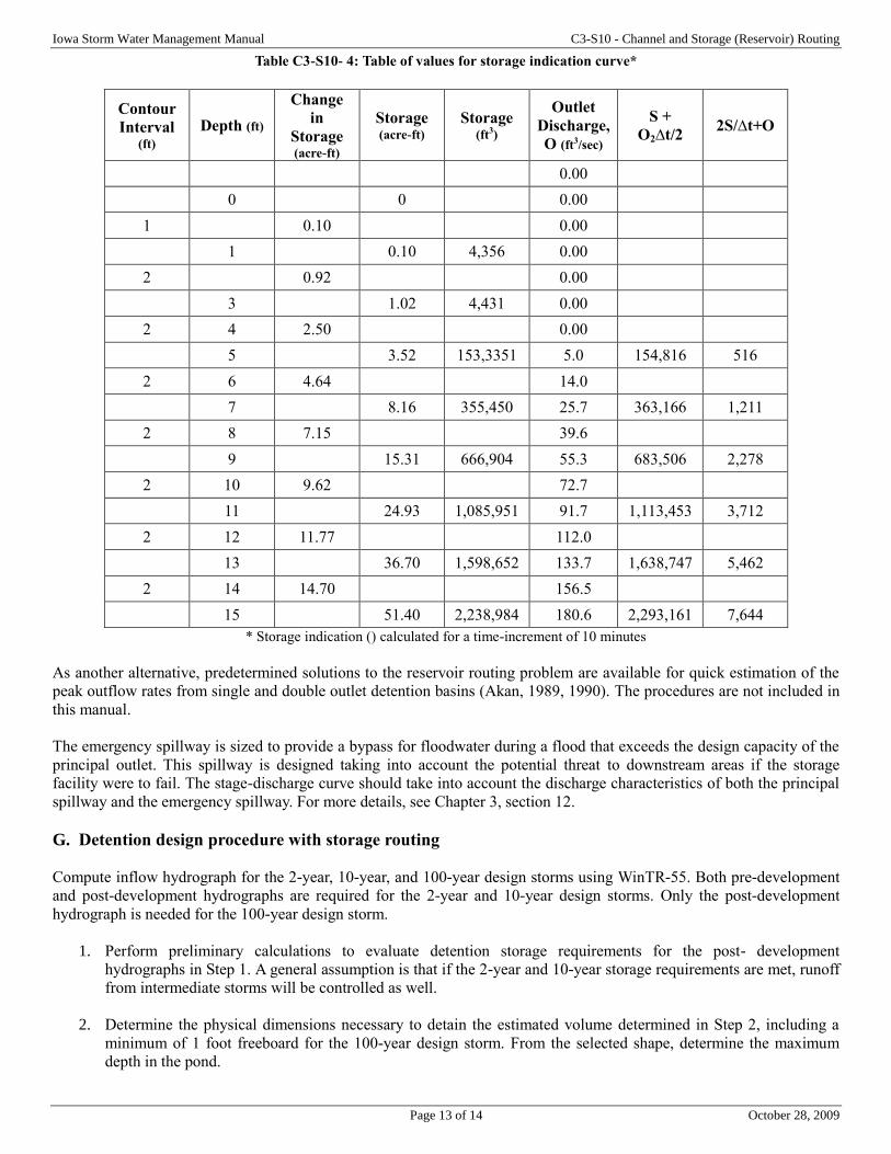
Iowa Storm Water Management Manual C3-S10 - Channel and Storage (Reservoir) Routing
Page 13 of 14 October 28, 2009
Table C3-S10- 4: Table of values for storage indication curve*
Contour
Interval (ft)
Depth (ft)
Change
in
Storage (acre-ft)
Storage (acre-ft)
Storage (ft3)
Outlet
Discharge,
O (ft3/sec)
S +
O2∆t/2 2S/∆t+O
0.00
0 0 0.00
1 0.10 0.00
1 0.10 4,356 0.00
2 0.92 0.00
3 1.02 4,431 0.00
2 4 2.50 0.00
5 3.52 153,3351 5.0 154,816 516
2 6 4.64 14.0
7 8.16 355,450 25.7 363,166 1,211
2 8 7.15 39.6
9 15.31 666,904 55.3 683,506 2,278
2 10 9.62 72.7
11 24.93 1,085,951 91.7 1,113,453 3,712
2 12 11.77 112.0
13 36.70 1,598,652 133.7 1,638,747 5,462
2 14 14.70 156.5
15 51.40 2,238,984 180.6 2,293,161 7,644
* Storage indication () calculated for a time-increment of 10 minutes
As another alternative, predetermined solutions to the reservoir routing problem are available for quick estimation of the
peak outflow rates from single and double outlet detention basins (Akan, 1989, 1990). The procedures are not included in
this manual.
The emergency spillway is sized to provide a bypass for floodwater during a flood that exceeds the design capacity of the
principal outlet. This spillway is designed taking into account the potential threat to downstream areas if the storage
facility were to fail. The stage-discharge curve should take into account the discharge characteristics of both the principal
spillway and the emergency spillway. For more details, see Chapter 3, section 12.
G. Detention design procedure with storage routing
Compute inflow hydrograph for the 2-year, 10-year, and 100-year design storms using WinTR-55. Both pre-development
and post-development hydrographs are required for the 2-year and 10-year design storms. Only the post-development
hydrograph is needed for the 100-year design storm.
1. Perform preliminary calculations to evaluate detention storage requirements for the post- development
hydrographs in Step 1. A general assumption is that if the 2-year and 10-year storage requirements are met, runoff
from intermediate storms will be controlled as well.
2. Determine the physical dimensions necessary to detain the estimated volume determined in Step 2, including a
minimum of 1 foot freeboard for the 100-year design storm. From the selected shape, determine the maximum
depth in the pond.

Iowa Storm Water Management Manual C3-S10 - Channel and Storage (Reservoir) Routing
Page 14 of 14 October 28, 2009
3. Select the type of outlet and size the outlet structure. The estimated peak stage will occur for the estimated peak
stage calculated in Step 2. The outlet structure is sized to convey the allowable discharge at this stage.
4. Perform the storage-indication routing calculation using the runoff hydrographs from Step 1 to check the
preliminary design using the storage routing procedure. If the routed post-development peak discharges from the
2-year and 10-year design events exceed the pre-development discharges, or if the peak stage varies significantly
from the estimated peak stage in Step 4, revise the estimated volume and repeat Step 3.
5. Complete a routing for the 100-year design storm through the basin and determine requirements for a secondary
spillway and check for minimum freeboard.
6. Evaluate downstream effects of the detention basin outflow to ensure the routed hydrograph does not increase
downstream flooding. The outflow hydrograph from the storage basin is routed through the downstream channel
until a confluence point is reached. The recommended criteria for locating the confluence point is where the
drainage area being analyzed represents 10% of the total drainage area.
7. Evaluate the outlet structure exit flow velocity, and provide channel and bank stabilization if the velocity will
cause channel degradation and erosion.
As noted in the discussion of the storage routing procedures, a significant number of modifications in storage
estimates, outlet structure configurations, and routing iterations may be necessary to achieve a suitable design. For
outlet structures controlling multiple design storm runoff events, the following general sizing criteria is provided
(Debo and Reese, 2002):
Generally, for the 2-year and 10-year design storms, the 10-year runoff volume will determine the size of
the detention basin, while the 2-year storm peak control requirement will determine the size of the
minimum outlet configuration.
Size the detention volume for the basin for the 10-year storm. The 2-year storm is then routed through the
basin, and the 2-year outlet structure is sized. If 2-year control is not required, then check the outlet sizing
for the 5-year storm.
In the case where multiple outlets are provided for WQv and Cpv, the lower orifice outlet for the Cpv will
also convey a portion of the outflow.
The depth of the storage when the 2-year (or 5-year) is routed through the basin, then establishes the invert
or weir elevation for the 10-year storm outlet. The 10-year through 50-year events are then routed through
both outlets.
H. Design example
Example detention basin design with routing
Page 1 of 4 October 28, 2009
Chapter 3- Section 11 Inlet Sediment Forebays
A. Introduction
A sediment forebay is a settling basin or plunge pool constructed at the incoming discharge points of a stormwater BMP.
The purpose of a sediment forebay is to allow sediment to settle from the incoming stormwater runoff before it is
delivered to the balance of the BMP. A sediment forebay helps to isolate the sediment deposition in an accessible area,
which facilitates BMP maintenance efforts. A sediment forebay is an essential component of most detention basins
infiltration BMPs, including dry and dry ED detention basins, wet detention basins, constructed wetlands, and infiltration
basins.
The sediment forebay is located at each inflow point in the stormwater BMP. Storm drain piping or other conveyances
may be aligned to discharge into one forebay, or several, as appropriate for the particular site. Forebays are installed in a
location which is accessible by maintenance equipment.
B. Water quality
A sediment forebay not only serves as a feature to reduce maintenance in the downstream stormwater BMP, it also
enhances the pollutant removal capabilities of the BMP. The volume and depth of the forebay work in concert with the
outlet protection at the inflow points to dissipate the energy of incoming stormwater flows. This allows heavier, coarse-
grained sediments and particulate pollutants to settle out of the runoff. For the BMPs listed in this handbook, the target
pollutant removal efficiencies have been established assuming sediment forebays are included in the design. Therefore, no
additional pollutant removal efficiency is warranted for using a sediment forebay.
C. Channel erosion control and flood control
An online BMP designed for flood control and channel protection volume (Cpv) is subject to the natural bed material
(sediment) load, plus any bed load increases due to higher velocities in the upstream channels. This is especially true for
regional facilities where the upstream channel is used to convey the increased developed condition flows. In such cases,
the sediment forebay becomes an essential facility maintenance component, since it serves to simplify clean-out
operations. A well-designed detention basin will function for 20-25 years before it needs dredging. This implies a gradual
sediment accumulation process.
The sediment forebay, however, is designed to trap the sediments within a confined area. This causes a more rapid
sediment accumulation. Studies indicate that for a typical mixed-use watershed, sediment removal from the forebay
should occur every 3-5 years. Despite this frequency, removal of sediment from the forebay should be less costly over the
same time period than a one-time cleaning of the entire basin. Removing sediment from the forebay is a much simpler
operation than cleaning the entire stormwater basin or pond. The sediment is confined to strategic forebay locations with
easy access. Furthermore, the more frequent and less expensive schedule can become a regular part of the operation and
maintenance efforts of the owners.
D. Design criteria
The most attractive aspect of a sediment forebay is its isolation from the rest of the facility. To create this separation, an
earthen berm, gabion, or concrete or riprap wall is constructed along the outlet side of the forebay. A designed overflow
section is constructed on the top of the separation to allow flow to exit the forebay at non-erosive velocities (<5 fps)
during the 2-year and 10-year frequency design storms. The overflow section is typically set at the permanent pool
elevation or the extended- detention volume elevation. It may also be designed to serve as a spillover for the forebay if the
forebay is set at a higher elevation than the second or remaining cell. The use of an aquatic bench with emergent
vegetation around the perimeter will help with water quality as well as provide a safety feature for large forebays (used on
large pond BMPs or retrofits).
1. Volume. The sediment forebay is sized for 0.25 inches of runoff per impervious acre of contributing drainage
area, with an absolute minimum of 0.1 inches per impervious acre. The volume of the sediment forebay is
considered part of the required volume of the detention basin permanent pool or extended detention volume. For
dry facilities, the forebay does not represent available storage volume if it remains full of water. A dry forebay
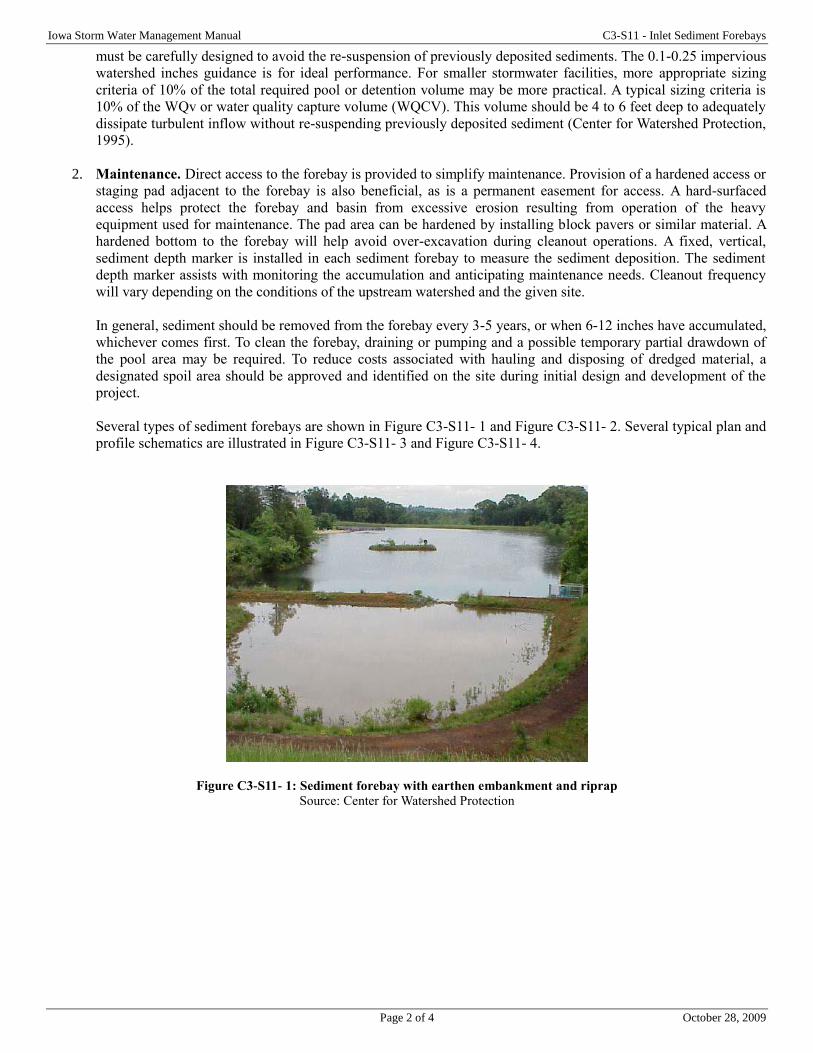
Iowa Storm Water Management Manual C3-S11 - Inlet Sediment Forebays
Page 2 of 4 October 28, 2009
must be carefully designed to avoid the re-suspension of previously deposited sediments. The 0.1-0.25 impervious
watershed inches guidance is for ideal performance. For smaller stormwater facilities, more appropriate sizing
criteria of 10% of the total required pool or detention volume may be more practical. A typical sizing criteria is
10% of the WQv or water quality capture volume (WQCV). This volume should be 4 to 6 feet deep to adequately
dissipate turbulent inflow without re-suspending previously deposited sediment (Center for Watershed Protection,
1995).
2. Maintenance. Direct access to the forebay is provided to simplify maintenance. Provision of a hardened access or
staging pad adjacent to the forebay is also beneficial, as is a permanent easement for access. A hard-surfaced
access helps protect the forebay and basin from excessive erosion resulting from operation of the heavy
equipment used for maintenance. The pad area can be hardened by installing block pavers or similar material. A
hardened bottom to the forebay will help avoid over-excavation during cleanout operations. A fixed, vertical,
sediment depth marker is installed in each sediment forebay to measure the sediment deposition. The sediment
depth marker assists with monitoring the accumulation and anticipating maintenance needs. Cleanout frequency
will vary depending on the conditions of the upstream watershed and the given site.
In general, sediment should be removed from the forebay every 3-5 years, or when 6-12 inches have accumulated,
whichever comes first. To clean the forebay, draining or pumping and a possible temporary partial drawdown of
the pool area may be required. To reduce costs associated with hauling and disposing of dredged material, a
designated spoil area should be approved and identified on the site during initial design and development of the
project.
Several types of sediment forebays are shown in Figure C3-S11- 1 and Figure C3-S11- 2. Several typical plan and
profile schematics are illustrated in Figure C3-S11- 3 and Figure C3-S11- 4.
Figure C3-S11- 1: Sediment forebay with earthen embankment and riprap
Source: Center for Watershed Protection
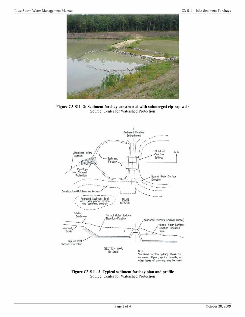
Iowa Storm Water Management Manual C3-S11 - Inlet Sediment Forebays
Page 3 of 4 October 28, 2009
Figure C3-S11- 2: Sediment forebay constructed with submerged rip-rap weir
Source: Center for Watershed Protection
Figure C3-S11- 3: Typical sediment forebay plan and profile
Source: Center for Watershed Protection
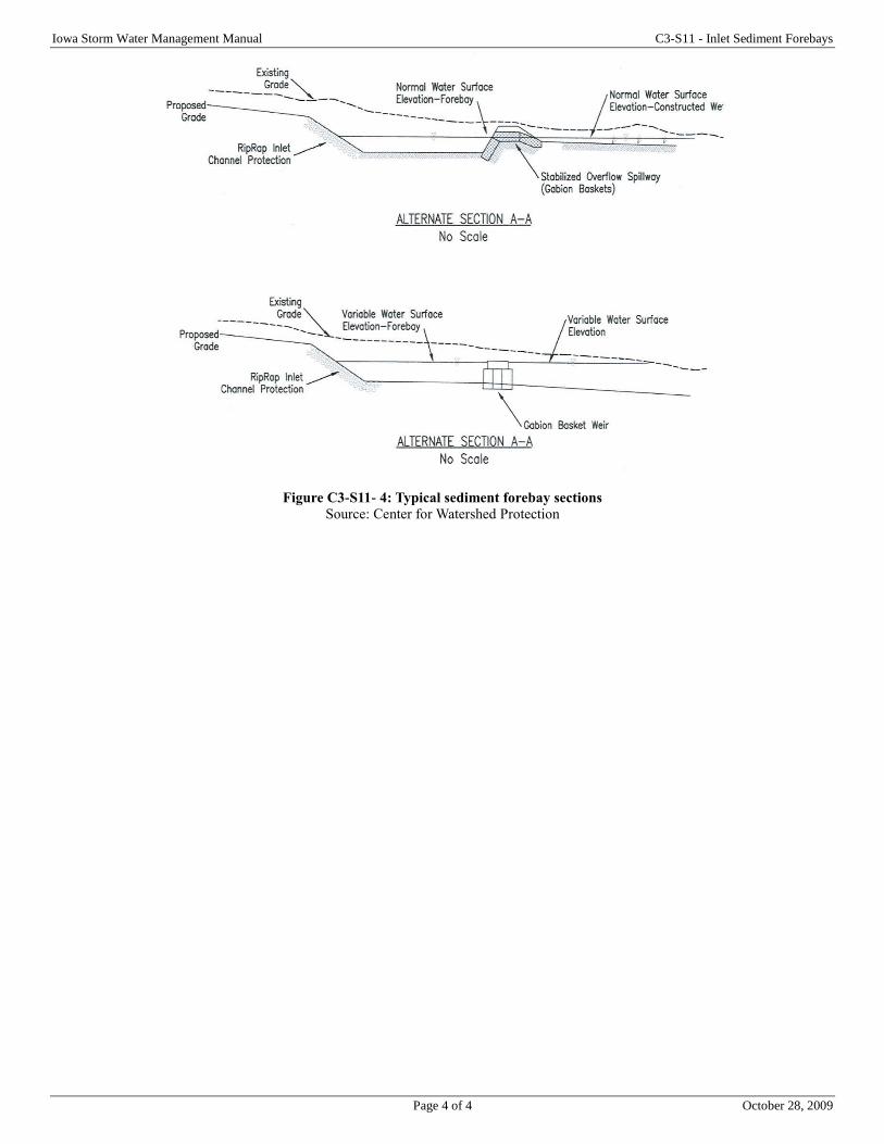
Iowa Storm Water Management Manual C3-S11 - Inlet Sediment Forebays
Page 4 of 4 October 28, 2009
Figure C3-S11- 4: Typical sediment forebay sections
Source: Center for Watershed Protection
Page 1 of 28 October 28, 2009
Chapter 3- Section 12 Detention Basin Outlet Structures
A. Introduction
The methods described in Chapter 3, section 9 are used to estimate the volume of the detention storage. The second step in
the design of the detention basin is determining the physical characteristics of the outlet structure. The outflow from a
detention basin depends on the type and the size of the outlet structure. A relationship between the stage and the discharge
can be determined from the hydraulics of these structures. Primary outlets provide the critical function of the regulation of
flow for structural stormwater controls. The outlet may be configured as a single outlet, or can be configured with
multiple outlet devices to provide multi-stage outlet control. For a single-stage system, the outlet can be designed as a
simple pipe or culvert. For multi-stage control structures, the inlet is designed considering a range of design flows. All
detention basins are designed with a secondary outlet, sometimes called an emergency or auxiliary spillway. The
secondary spillway is provided to convey the release of the maximum runoff discharge for the 100-year storm event. The
secondary spillway is most often a weir-type control, separate from the primary outlet structure and configured as part of
the detention basin embankment.
A stage-discharge curve is developed for the full range of flows that the structure would experience. The outlets are
housed in a riser structure connected to a single outlet conduit. An alternative approach would be to provide several pipe
or culvert outlets at different levels in the basin that are either discharged separately, or are combined to discharge at a
single location. This section provides an overview of outlet structure hydraulics and design for stormwater detention
facilities. The designer is referred to an appropriate hydraulics text for additional information on outlet structures not
contained in this section.
B. Outlet structure types
The most common types of outlets can be categorized into three groups: orifice-type, weir-type, and riser-pipe structures.
There are a wide variety of outlet structure types, the most common of which are covered in this section. Descriptions and
equations are provided for the following outlet types for use in stormwater facility design:
Orifices
Perforated risers
Pipes/culverts
Sharp-crested weirs
Broad-crested weirs
V-notch weirs
Proportional weirs
Combination outlets
Each of these outlet types has a different design purpose and application:
Water quality and channel protection flows are normally handled with smaller, more protected outlet structures,
such as reverse slope pipes, hooded orifices, orifices located within screened pipes or risers, perforated plates or
risers, and V-notch weirs.
Larger flows, such as overbank protection and extreme flood flows, are typically handled through a riser with
different-sized openings, through an overflow at the top of a riser (drop inlet structure), or a flow over a broad
crested weir or spillway through the embankment. Overflow weirs can also be of different heights and
configurations to handle control of multiple design flows.
1. Orifices. An orifice is a circular or rectangular opening of a prescribed shape and size. The flow rate depends on
the height of the water above the opening and the size and edge treatment of the orifice. For a single orifice, as
illustrated in Figure C3-S12- 1, the orifice discharge can be determined using the standard orifice equation below.
Equation C3-S12- 1
𝑄 − 𝐶𝐴0(2𝑔ℎ)0.5
Iowa Storm Water Management Manual C3-S12 - Detention Basin Outlet Structures
Page 2 of 28 October 28, 2009
Where:
Q = the orifice flow discharge (cfs)
Cd = dimensionless coefficient of discharge
A0 = cross-sectional area of orifice or pipe (ft2)
g = acceleration due to gravity (32.2 ft/sec2)
Do = diameter of orifice or pipe (ft)
h = effective head on the orifice, from the center of orifice to the water surface
Equation C3-S12- 1a
For circular orifices:
𝐴0 =𝜋𝐷𝑜
2
4
Equation C3-S12- 1b
For rectangular orifices:
𝐴0 = 𝑏𝐷
Where:
b and D represent the side lengths of the rectangular opening
Typical values for Cd are 0.6 for square edge uniform entrance conditions, and 0.4 for ragged edge orifices
(FHWA, 1996).
If the orifice discharges as a free outfall, then the effective head is measured from the center of the orifice to the
upstream (headwater) surface elevation. If the orifice discharge is submerged, then the effective head is the
difference in elevation of the headwater and tailwater surfaces as shown in Figure C3-S12- 1.
Figure C3-S12- 1: Orifice outlets
2. Weir-type outlets. Rectangular broad-crested weirs, overflow spillways and sharp-crested weirs are included in
this group. The discharge over these structures (Figure C3-S12- 2) is determined using the general form of the
equation (Brater and King, 1976).
Equation C3-S12- 2
𝑄 = 𝐶𝑊𝐿(2𝑔ℎ)3 2⁄
Where:
Cw = dimensionless weir discharge coefficient
L = effective weir length, ft
H = water depth above the crest
Iowa Storm Water Management Manual C3-S12 - Detention Basin Outlet Structures
Page 3 of 28 October 28, 2009
Figure C3-S12- 2: Weir outlet
3. Broad-crested weirs. A weir in the form of a relatively long raised channel control crest section is a broad-
crested weir. The flow control section can have different shapes, such as triangular or circular. True broad-crested
weir flow will occur when upstream head above the crest is between the limits of about 1/20 and ½ the crest length
in the direction of flow (USBR, 1997). If the upstream edge of a broad-crested weir is so rounded as to prevent
contraction, and if the slope of the crest is as great as the loss of head due to friction, flow will pass through
critical depth at the weir crest; this gives the maximum C value of 3.087. For sharp corners on the broad-crested
weir, a minimum C value of 2.6 should be used. Information on C values as a function of weir crest breadth and
head is given in Table C3-S12- 1.
Table C3-S12- 1: Broad-crested weir coefficient (Cw) values
Head (h)1
(feet) Weir Crest Breadth (b) (feet)
0.50 0.75 1.00 1.50 2.00 2.50 3.00 4.00 5.00 10.00 15.00
0.2 2.80 2.75 2.69 2.62 2.54 2.48 2.44 2.38 2.34 2.49 2.68
0.4 2.92 2.80 2.72 2.64 2.61 2.60 2.58 2.54 2.50 2.56 2.70
0.6 3.08 2.89 2.75 2.64 2.61 2.60 2.68 2.69 2.70 2.70 2.70
0.8 3.30 3.04 2.85 2.68 2.60 2.60 2.67 2.68 2.68 2.69 2.64
1.0 3.32 3.14 2.98 2.75 2.66 2.64 2.65 2.67 2.68 2.68 2.63
1.2 3.32 3.20 3.08 2.86 2.70 2.65 2.64 2.67 2.66 2.69 2.64
1.4 3.32 3.26 3.20 2.92 2.77 2.68 2.64 2.64 2.65 2.67 2.64
1.6 3.32 3.29 3.28 3.07 2.89 2.75 2.68 2.66 2.65 2.64 2.63
1.8 3.32 3.32 3.31 3.07 2.88 2.74 2.68 2.66 2.65 2.64 2.63
2.0 3.32 3.31 3.30 3.03 2.85 2.76 2.27 2.68 2.65 2.64 2.63
2.5 3.32 3.32 3.31 3.28 3.07 2.89 2.81 2.72 2.67 2.64 2.63
3.0 3.32 3.32 3.32 3.32 3.20 3.05 2.92 2.73 2.66 2.64 2.63
3.5 3.32 3.32 3.32 3.32 3.32 3.19 2.97 2.76 2.68 2.64 2.63
4.0 3.32 3.32 3.32 3.32 3.32 3.32 3.07 2.79 2.70 2.64 2.63
4.5 3.32 3.32 3.32 3.32 3.32 3.32 3.32 2.88 2.74 2.64 2.63
5.0 3.32 3.32 3.32 3.32 3.32 3.32 3.32 3.07 2.79 2.64 2.63
5.5 3.32 3.32 3.32 3.32 3.32 3.32 3.32 3.32 2.88 2.64 2.63 1Measured at least 2.5h upstream of the weir
Iowa Storm Water Management Manual C3-S12 - Detention Basin Outlet Structures
Page 4 of 28 October 28, 2009
4. V-notch weirs. The discharge through a V-notch weir (Figure C3-S12- 3) can be calculated from the following
equation (Brater and King, 1976).
Equation C3-S12- 3
𝑄 = 2.5 tan (𝜃
2) ℎ2.5
Where:
Q = discharge (cfs)
θ = angle of V-notch (degrees)
H = head on apex of notch (ft)
Figure C3-S12- 3: V-notch weir
For a 60° V-notch weir: 𝑄 − 4.33ℎ2.5
For a 90° V-notch weir: 𝑄 = 2.5ℎ2.5
5. Cipoletti (trapezoidal) weir. The Cipoletti (or trapezoidal) weir has side slopes in the vertical to horizontal ratio
of 4:1. Cipoletti weirs are considered fully contracted, and are installed as described below. The discharge
coefficient for Cipoletti weirs is 3.367 (in English units), and it does not depend on L or P as for the rectangular
weir. The discharge coefficient formulation is simpler than for rectangular weirs, but the accuracy is somewhat
decreased – about ±5% (USBR, 1997). The Cipoletti weir equation is shown below for Q in cfs (ft3/s), and head
and length in feet units (USBR, 1997).
Equation C3-S12- 4
𝑄 = 3.367𝐿ℎ3
2⁄
Where:
Q = discharge (cfs)
L = weir length (ft)
h = depth of water above crest (ft)
Note that L is measured along the bottom of the weir crest (not along the water surface). Weir side slopes should
have a vertical to horizontal ratio of 4:1. Head (h) should be measured at a distance of at least 4h upstream of the
weir.
Iowa Storm Water Management Manual C3-S12 - Detention Basin Outlet Structures
Page 5 of 28 October 28, 2009
Figure C3-S12- 4: Cipoletti (trapezoidal) weir
It doesn't matter how thick the weir is, except where water flows through the weir. The weir should be between
0.03 and 0.08 inches thick in the opening. If the bulk of the weir is thicker than 0.08 inch, the downstream edge of
the opening can be chambered at an angle greater than 45° (60° is recommended) to achieve the desired thickness
of the edges. Water surface downstream of the weir should be at least 0.2 feet below the weir crest (i.e. below the
bottom of the opening).
Measured head (h) should be greater than 0.2 feet, but less than L/3. P is measured from the bottom of the
upstream channel, and should be greater than 2hmax, where hmax is the maximum expected head. b is measured
from the sides of the channel and also should be greater than 2hmax.
6. Pipes and culverts. Discharge pipes are often used as outlet structures for stormwater control facilities. The
design of these pipes can be for either single or multi-stage discharges. A reverse- slope underwater pipe is often
used for water quality or channel protection outlets. Pipes smaller than 12 inches in diameter may be analyzed as
a submerged orifice as long as H/D is greater than 1.5. Note: For low-flow conditions, when the flow reaches and
begins to overflow the pipe, weir flow controls the hydraulics. The flow will transition to orifice flow as the stage
increases above the top of the opening.
Pipes greater than 12 inches in diameter should be analyzed as a discharge pipe with headwater and tailwater
effects taken into account. The outlet hydraulics for pipe flow can be determined from the outlet control culvert
nomographs and procedures given in Chapter 14, or by using Equation C3-S12- 5 (NRCS, 1984). The following
equation is a general pipe flow equation that is derived through the use of the Bernoulli and continuity principles.
Equation C3-S12- 5
𝑄 = 𝐴𝑝 [2𝑔ℎ
1 + 𝑘𝑚 + 𝑘𝑝𝐿]
0.5
Where:
Q = discharge (cfs)
Ap = pipe cross sectional area (ft2) g = acceleration of gravity (ft/s2)
H = elevation head differential (ft)
km = coefficient of minor losses (use 1.0)
kp = pipe friction coefficient = 5087𝑛2 𝐷4 3⁄⁄ (Manning’s n and pipe diameter, D)
L = pipe length (ft)
7. Proportional weirs. Although more complex to design and construct, a proportional weir may significantly
reduce the required storage volume for a given site. The proportional weir is distinguished from other control
devices by having a linear head-discharge relationship achieved by allowing the discharge area to vary non-
linearly with head. A typical proportional weir is shown in Figure C3-S12- 5. Design equations for proportional
weirs are (Sandvik, 1985):
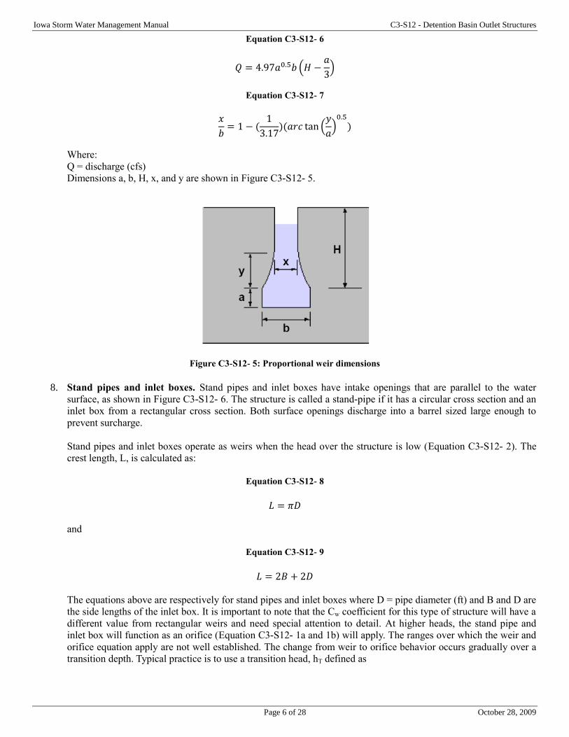
Iowa Storm Water Management Manual C3-S12 - Detention Basin Outlet Structures
Page 6 of 28 October 28, 2009
Equation C3-S12- 6
𝑄 = 4.97𝑎0.5𝑏 (𝐻 −𝑎
3)
Equation C3-S12- 7
𝑥
𝑏= 1 − (
1
3.17)(𝑎𝑟𝑐 tan (
𝑦
𝑎)
0.5
)
Where:
Q = discharge (cfs)
Dimensions a, b, H, x, and y are shown in Figure C3-S12- 5.
Figure C3-S12- 5: Proportional weir dimensions
8. Stand pipes and inlet boxes. Stand pipes and inlet boxes have intake openings that are parallel to the water
surface, as shown in Figure C3-S12- 6. The structure is called a stand-pipe if it has a circular cross section and an
inlet box from a rectangular cross section. Both surface openings discharge into a barrel sized large enough to
prevent surcharge.
Stand pipes and inlet boxes operate as weirs when the head over the structure is low (Equation C3-S12- 2). The
crest length, L, is calculated as:
Equation C3-S12- 8
𝐿 = 𝜋𝐷
and
Equation C3-S12- 9
𝐿 = 2𝐵 + 2𝐷
The equations above are respectively for stand pipes and inlet boxes where D = pipe diameter (ft) and B and D are
the side lengths of the inlet box. It is important to note that the Cw coefficient for this type of structure will have a
different value from rectangular weirs and need special attention to detail. At higher heads, the stand pipe and
inlet box will function as an orifice (Equation C3-S12- 1a and 1b) will apply. The ranges over which the weir and
orifice equation apply are not well established. The change from weir to orifice behavior occurs gradually over a
transition depth. Typical practice is to use a transition head, hT defined as
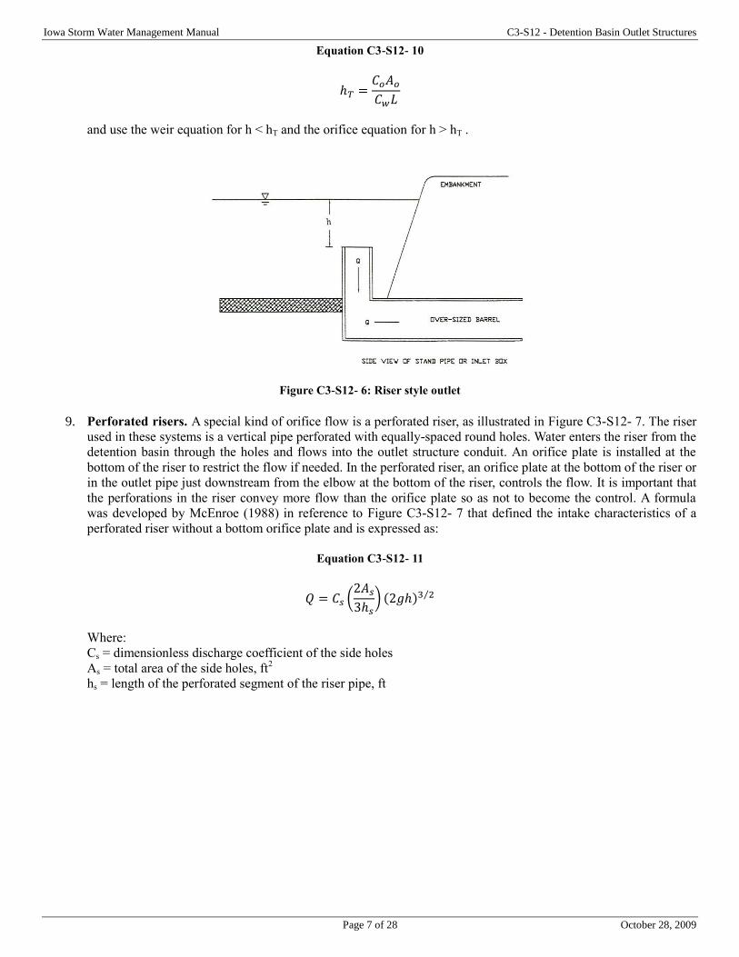
Iowa Storm Water Management Manual C3-S12 - Detention Basin Outlet Structures
Page 7 of 28 October 28, 2009
Equation C3-S12- 10
ℎ𝑇 =𝐶𝑜𝐴𝑜
𝐶𝑤𝐿
and use the weir equation for h < hT and the orifice equation for h > hT .
Figure C3-S12- 6: Riser style outlet
9. Perforated risers. A special kind of orifice flow is a perforated riser, as illustrated in Figure C3-S12- 7. The riser
used in these systems is a vertical pipe perforated with equally-spaced round holes. Water enters the riser from the
detention basin through the holes and flows into the outlet structure conduit. An orifice plate is installed at the
bottom of the riser to restrict the flow if needed. In the perforated riser, an orifice plate at the bottom of the riser or
in the outlet pipe just downstream from the elbow at the bottom of the riser, controls the flow. It is important that
the perforations in the riser convey more flow than the orifice plate so as not to become the control. A formula
was developed by McEnroe (1988) in reference to Figure C3-S12- 7 that defined the intake characteristics of a
perforated riser without a bottom orifice plate and is expressed as:
Equation C3-S12- 11
𝑄 = 𝐶𝑠 (2𝐴𝑠
3ℎ𝑠) (2𝑔ℎ)3 2⁄
Where:
Cs = dimensionless discharge coefficient of the side holes
As = total area of the side holes, ft2
hs = length of the perforated segment of the riser pipe, ft
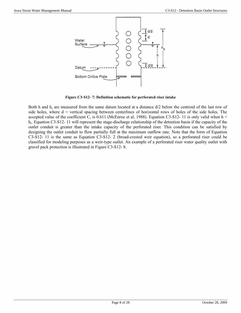
Iowa Storm Water Management Manual C3-S12 - Detention Basin Outlet Structures
Page 8 of 28 October 28, 2009
Figure C3-S12- 7: Definition schematic for perforated riser intake
Both h and hs are measured from the same datum located at a distance d/2 below the centroid of the last row of
side holes, where d = vertical spacing between centerlines of horizontal rows of holes of the side holes. The
accepted value of the coefficient Cs is 0.611 (McEnroe et al, 1988). Equation C3-S12- 11 is only valid when h <
hs. Equation C3-S12- 11 will represent the stage-discharge relationship of the detention basin if the capacity of the
outlet conduit is greater than the intake capacity of the perforated riser. This condition can be satisfied by
designing the outlet conduit to flow partially full at the maximum outflow rate. Note that the form of Equation
C3-S12- 11 is the same as Equation C3-S12- 2 (broad-crested weir equation), so a perforated riser could be
classified for modeling purposes as a weir-type outlet. An example of a perforated riser water quality outlet with
gravel pack protection is illustrated in Figure C3-S12- 8.
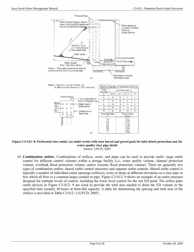
Iowa Storm Water Management Manual C3-S12 - Detention Basin Outlet Structures
Page 9 of 28 October 28, 2009
Figure C3-S12- 8: Perforated riser outlet: (a) outlet works with riser barrel and gravel pack for inlet debris protection and (b)
water quality riser pipe detail
Source: UFCD, 2005
10. Combination outlets. Combinations of orifices, weirs, and pipes can be used to provide multi- stage outlet
control for different control volumes within a storage facility (i.e., water quality volume, channel protection
volume, overbank flood protection volume, and/or extreme flood protection volume). There are generally two
types of combination outlets: shared outlet control structures and separate outlet controls. Shared outlet control is
typically a number of individual outlet openings (orifices), weirs or drops at different elevations on a riser pipe or
box which all flow to a common larger conduit or pipe. Figure C3-S12- 9 shows an example of an outlet structure
designed for multiple levels of control, including the lower level control for the wet ED pond. The orifice plate
outlet devices in Figure C3-S12- 9 are sized to provide the total area needed to drain the ED volume in the
specified time (usually 40 hours at brim-full capacity. A table for determining the spacing and total area of the
orifices is provided in Table C3-S12- 2 (UFCD, 2005).
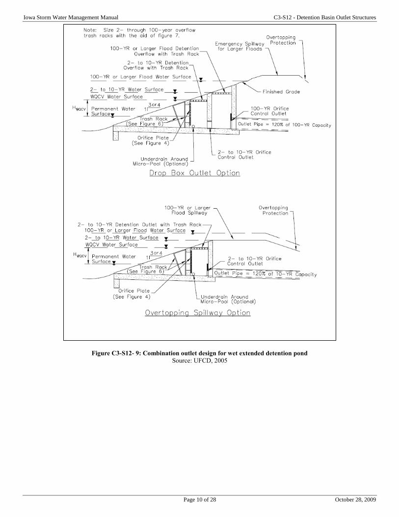
Iowa Storm Water Management Manual C3-S12 - Detention Basin Outlet Structures
Page 10 of 28 October 28, 2009
Figure C3-S12- 9: Combination outlet design for wet extended detention pond
Source: UFCD, 2005
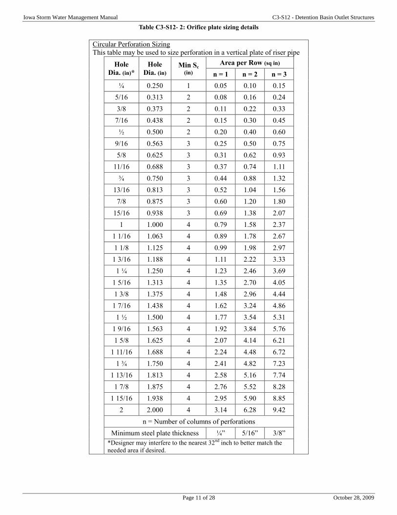
Iowa Storm Water Management Manual C3-S12 - Detention Basin Outlet Structures
Page 11 of 28 October 28, 2009
Table C3-S12- 2: Orifice plate sizing details
Circular Perforation Sizing
This table may be used to size perforation in a vertical plate of riser pipe
Hole
Dia. (in)*
Hole
Dia. (in) Min Sc
(in)
Area per Row (sq in)
n = 1 n = 2 n = 3
¼ 0.250 1 0.05 0.10 0.15
5/16 0.313 2 0.08 0.16 0.24
3/8 0.373 2 0.11 0.22 0.33
7/16 0.438 2 0.15 0.30 0.45
½ 0.500 2 0.20 0.40 0.60
9/16 0.563 3 0.25 0.50 0.75
5/8 0.625 3 0.31 0.62 0.93
11/16 0.688 3 0.37 0.74 1.11
¾ 0.750 3 0.44 0.88 1.32
13/16 0.813 3 0.52 1.04 1.56
7/8 0.875 3 0.60 1.20 1.80
15/16 0.938 3 0.69 1.38 2.07
1 1.000 4 0.79 1.58 2.37
1 1/16 1.063 4 0.89 1.78 2.67
1 1/8 1.125 4 0.99 1.98 2.97
1 3/16 1.188 4 1.11 2.22 3.33
1 ¼ 1.250 4 1.23 2.46 3.69
1 5/16 1.313 4 1.35 2.70 4.05
1 3/8 1.375 4 1.48 2.96 4.44
1 7/16 1.438 4 1.62 3.24 4.86
1 ½ 1.500 4 1.77 3.54 5.31
1 9/16 1.563 4 1.92 3.84 5.76
1 5/8 1.625 4 2.07 4.14 6.21
1 11/16 1.688 4 2.24 4.48 6.72
1 ¾ 1.750 4 2.41 4.82 7.23
1 13/16 1.813 4 2.58 5.16 7.74
1 7/8 1.875 4 2.76 5.52 8.28
1 15/16 1.938 4 2.95 5.90 8.85
2 2.000 4 3.14 6.28 9.42
n = Number of columns of perforations
Minimum steel plate thickness ¼” 5/16” 3/8”
*Designer may interfere to the nearest 32
nd inch to better match the
needed area if desired.

Iowa Storm Water Management Manual C3-S12 - Detention Basin Outlet Structures
Page 12 of 28 October 28, 2009
Rectangular Perforation Sizing
Use only one rectangular column
whenever two 2-in diameter
circular perforations cannot
provide needed outlet area.
Rectangular
Hole Width (in)
Min Steel
Thickness (in)
5 ¼
6 ¼
7 5/32
Rectangular Height = 2” 8 5/16
Rectangular Width = Required
Area per Row / 2” 9 11/32
10 3/8
>10 ½
Source: UFCD, 2005
C. Extended detention (water quality and channel protection) outlet design
Extended detention orifice sizing is required in design applications that provide extended detention for downstream
channel protection or the ED portion of the water quality volume. In both cases, an extended detention orifice or reverse
slope pipe can be used for the outlet. For a structural control facility providing both WQv extended detention and Cpv
control (wet ED pond, micropool ED pond, and shallow ED wetland), there will be a need to design two outlet orifices –
one for the water quality control outlet and one for the channel protection drawdown.
The outlet hydraulics for peak control design (overbank flood protection and extreme flood protection) is usually
straightforward in that an outlet is selected that will limit the peak flow to some pre-determined maximum. Since volume
and the time required for water to exit the storage facility are not usually considered, the outlet design can easily be
calculated and routing procedures used to determine if quantity design criteria are met.
In an extended detention facility for water quality treatment or downstream channel protection, however, the storage
volume is detained and released over a specified amount of time (e.g., 24 hours). The release period is a brim drawdown
time, beginning at the time of peak storage of the water quality volume until the entire calculated volume drains out of the
basin. This assumes that the brim volume is present in the basin prior to any discharge. In reality, however, water is
flowing out of the basin prior to the full or brim volume being reached. Therefore, the extended detention outlet can be
sized using either of the following methods. The WQv is determined by the procedures included in Chapter 3, section 6
with the water quality capture volume (WQCV) being the preferred method for extended detention basins (ASCE/WEF
method). A minimum drawdown time (detention time) of 24 hours should be used. Water quality performance will
improve as the brim-full detention time approaches 40 hours.
The following procedures are based on the water quality outlet design procedures included in the Virginia Stormwater
Management Handbook, 1999.
Use the maximum hydraulic head associated with the storage volume and maximum flow, and calculate the
orifice size needed to achieve the required drawdown time; and route the volume through the basin to verify the
actual storage volume used and the drawdown time.
Approximate the orifice size using the average hydraulic head associated with the storage volume and the required
drawdown time. These two procedures are outlined in the examples below, and can be used to size an extended
detention orifice for water quality and/or channel protection.
1. Method 1: maximum hydraulic head with routing. A wet ED pond sized for the required water quality volume
will be used here to illustrate the sizing procedure for an extended-detention orifice. Given the following
information, calculate the required orifice size for water quality design.
Given: water quality volume (WQv) = 0.76 ac-ft = 33,106 ft3 Maximum hydraulic head (Hmax) = 5.0 ft (from stage
vs. storage data)
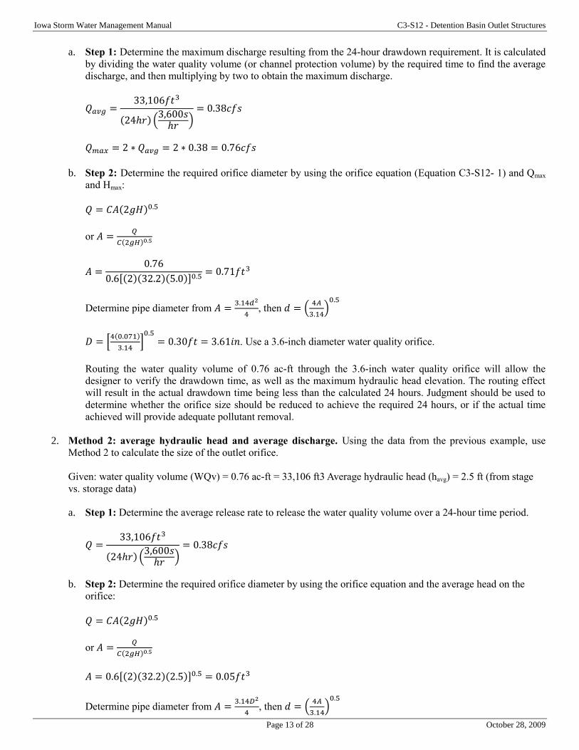
Iowa Storm Water Management Manual C3-S12 - Detention Basin Outlet Structures
Page 13 of 28 October 28, 2009
a. Step 1: Determine the maximum discharge resulting from the 24-hour drawdown requirement. It is calculated
by dividing the water quality volume (or channel protection volume) by the required time to find the average
discharge, and then multiplying by two to obtain the maximum discharge.
𝑄𝑎𝑣𝑔 =33,106𝑓𝑡3
(24ℎ𝑟) (3,600𝑠
ℎ𝑟)
= 0.38𝑐𝑓𝑠
𝑄𝑚𝑎𝑥 = 2 ∗ 𝑄𝑎𝑣𝑔 = 2 ∗ 0.38 = 0.76𝑐𝑓𝑠
b. Step 2: Determine the required orifice diameter by using the orifice equation (Equation C3-S12- 1) and Qmax
and Hmax:
𝑄 = 𝐶𝐴(2𝑔𝐻)0.5
or 𝐴 =𝑄
𝐶(2𝑔𝐻)0.5
𝐴 =0.76
0.6[(2)(32.2)(5.0)]0.5= 0.71𝑓𝑡3
Determine pipe diameter from 𝐴 =3.14𝑑2
4, then 𝑑 = (
4𝐴
3.14)
0.5
𝐷 = [4(0.071)
3.14]
0.5= 0.30𝑓𝑡 = 3.61𝑖𝑛. Use a 3.6-inch diameter water quality orifice.
Routing the water quality volume of 0.76 ac-ft through the 3.6-inch water quality orifice will allow the
designer to verify the drawdown time, as well as the maximum hydraulic head elevation. The routing effect
will result in the actual drawdown time being less than the calculated 24 hours. Judgment should be used to
determine whether the orifice size should be reduced to achieve the required 24 hours, or if the actual time
achieved will provide adequate pollutant removal.
2. Method 2: average hydraulic head and average discharge. Using the data from the previous example, use
Method 2 to calculate the size of the outlet orifice.
Given: water quality volume (WQv) = 0.76 ac-ft = 33,106 ft3 Average hydraulic head (havg) = 2.5 ft (from stage
vs. storage data)
a. Step 1: Determine the average release rate to release the water quality volume over a 24-hour time period.
𝑄 =33,106𝑓𝑡3
(24ℎ𝑟) (3,600𝑠
ℎ𝑟)
= 0.38𝑐𝑓𝑠
b. Step 2: Determine the required orifice diameter by using the orifice equation and the average head on the
orifice:
𝑄 = 𝐶𝐴(2𝑔𝐻)0.5
or 𝐴 =𝑄
𝐶(2𝑔𝐻)0.5
𝐴 = 0.6[(2)(32.2)(2.5)]0.5 = 0.05𝑓𝑡3
Determine pipe diameter from 𝐴 =3.14𝐷2
4, then 𝑑 = (
4𝐴
3.14)
0.5
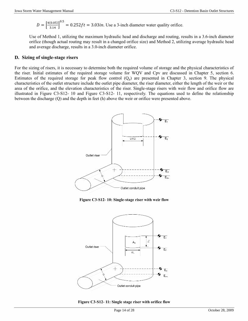
Iowa Storm Water Management Manual C3-S12 - Detention Basin Outlet Structures
Page 14 of 28 October 28, 2009
𝐷 = [4(0.05)
3.14]
0.5= 0.252𝑓𝑡 = 3.03𝑖𝑛. Use a 3-inch diameter water quality orifice.
Use of Method 1, utilizing the maximum hydraulic head and discharge and routing, results in a 3.6-inch diameter
orifice (though actual routing may result in a changed orifice size) and Method 2, utilizing average hydraulic head
and average discharge, results in a 3.0-inch diameter orifice.
D. Sizing of single-stage risers
For the sizing of risers, it is necessary to determine both the required volume of storage and the physical characteristics of
the riser. Initial estimates of the required storage volume for WQV and Cpv are discussed in Chapter 5, section 6.
Estimates of the required storage for peak flow control (Qp) are presented in Chapter 3, section 9. The physical
characteristics of the outlet structure include the outlet pipe diameter, the riser diameter, either the length of the weir or the
area of the orifice, and the elevation characteristics of the riser. Single-stage risers with weir flow and orifice flow are
illustrated in Figure C3-S12- 10 and Figure C3-S12- 11, respectively. The equations used to define the relationship
between the discharge (Q) and the depth in feet (h) above the weir or orifice were presented above.
Figure C3-S12- 10: Single-stage riser with weir flow
Figure C3-S12- 11: Single stage riser with orifice flow
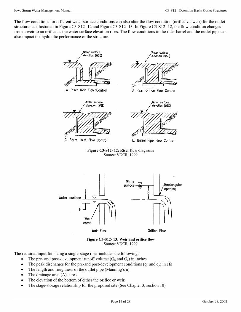
Iowa Storm Water Management Manual C3-S12 - Detention Basin Outlet Structures
Page 15 of 28 October 28, 2009
The flow conditions for different water surface conditions can also alter the flow condition (orifice vs. weir) for the outlet
structure, as illustrated in Figure C3-S12- 12 and Figure C3-S12- 13. In Figure C3-S12- 12, the flow condition changes
from a weir to an orifice as the water surface elevation rises. The flow conditions in the rider barrel and the outlet pipe can
also impact the hydraulic performance of the structure.
Figure C3-S12- 12: Riser flow diagrams
Source: VDCR, 1999
Figure C3-S12- 13: Weir and orifice flow
Source: VDCR, 1999
The required input for sizing a single-stage riser includes the following:
The pre- and post-development runoff volume (Qb and Qa) in inches
The peak discharges for the pre-and post-development conditions (qb and qa) in cfs
The length and roughness of the outlet pipe (Manning’s n)
The drainage area (A) acres
The elevation of the bottom of either the orifice or weir.
The stage-storage relationship for the proposed site (See Chapter 3, section 10)
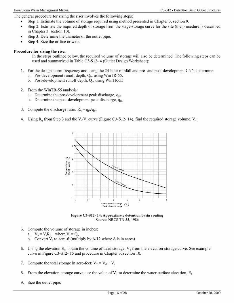
Iowa Storm Water Management Manual C3-S12 - Detention Basin Outlet Structures
Page 16 of 28 October 28, 2009
The general procedure for sizing the riser involves the following steps:
Step 1: Estimate the volume of storage required using method presented in Chapter 3, section 9.
Step 2: Estimate the required depth of storage from the stage-storage curve for the site (the procedure is described
in Chapter 3, section 10).
Step 3: Determine the diameter of the outlet pipe.
Step 4: Size the orifice or weir.
Procedure for sizing the riser
In the steps outlined below, the required volume of storage will also be determined. The following steps can be
used and summarized in Table C3-S12- 4 (Outlet Design Worksheet):
1. For the design storm frequency and using the 24-hour rainfall and pre- and post-development CN’s, determine:
a. Pre-development runoff depth, Qb, using WinTR-55.
b. Post-development runoff depth, Qa, using WinTR-55.
2. From the WinTR-55 analysis:
a. Determine the pre-development peak discharge, qpb.
b. Determine the post-development peak discharge, qpa.
3. Compute the discharge ratio: Rq = qpb/qpa
4. Using Rq from Step 3 and the Vs/Vr curve (Figure C3-S12- 14), find the required storage volume, Vs:
Figure C3-S12- 14: Approximate detention basin routing
Source: NRCS TR-55, 1986
5. Compute the volume of storage in inches:
a. Vs = VrRq where Vr = Qa
b. Convert Vs to acre-ft (multiply by A/12 where A is in acres)
6. Using the elevation E0, obtain the volume of dead storage, Vd from the elevation-storage curve. See example
curve in Figure C3-S12- 15 and procedure in Chapter 3, section 10.
7. Compute the total storage in acre-feet: VT = Vd + Vs
8. From the elevation-storage curve, use the value of VT to determine the water surface elevation, E1.
9. Size the outlet pipe:
Iowa Storm Water Management Manual C3-S12 - Detention Basin Outlet Structures
Page 17 of 28 October 28, 2009
a. Obtain the friction head loss coefficient Kp from Table C3-S12- 3.
b. Using the product LKp, obtain C* from
c. Figure C3-S12- 15 where L is length of the conduit pipe.
Table C3-S12- 3: Kp values for RCP (n=0.013) and CMP (n= 0.024)*
Pipe
Diameter (in) RCP CMP
12 0.03129 0.10665
18 0.01822 0.06211
24 0.01242 0.04233
30 0.01061 0.03617
27 0.00922 0.03143
36 0.00723 0.02465
42 0.00589 0.02007
48 0.00493 0.01680
54 0.00421 0.01436
60 0.00366 0.01247
72 0.00287 0.00978 *For other values of n and D, Kp can be calculated by
𝐾𝑝 = 5087𝑛2𝐷−4.3
Figure C3-S12- 15: Conduit diameter coefficient C*
Source: Chow
10. If the outlet is an orifice determine the characteristics of the orifice:
a. Set the orifice width, Wo; as a starting value use 0.75D
b. Compute the required area, Ao: Ao = 0.2283qpb/(E1-E0)0.5
c. Compute the height: Ho = Ao / Wo
11. If the outlet is a weir, determine the characteristics of the weir length: Lw = qpb/3.1(E1-E0)1.5
12. Determine the conduit invert elevation (ft) at the face of the riser: Einv = Ec – D/2
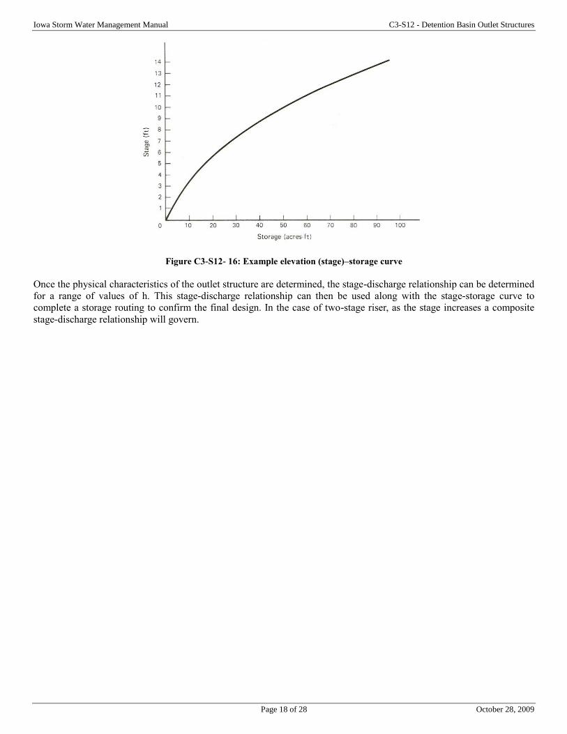
Iowa Storm Water Management Manual C3-S12 - Detention Basin Outlet Structures
Page 18 of 28 October 28, 2009
Figure C3-S12- 16: Example elevation (stage)–storage curve
Once the physical characteristics of the outlet structure are determined, the stage-discharge relationship can be determined
for a range of values of h. This stage-discharge relationship can then be used along with the stage-storage curve to
complete a storage routing to confirm the final design. In the case of two-stage riser, as the stage increases a composite
stage-discharge relationship will govern.
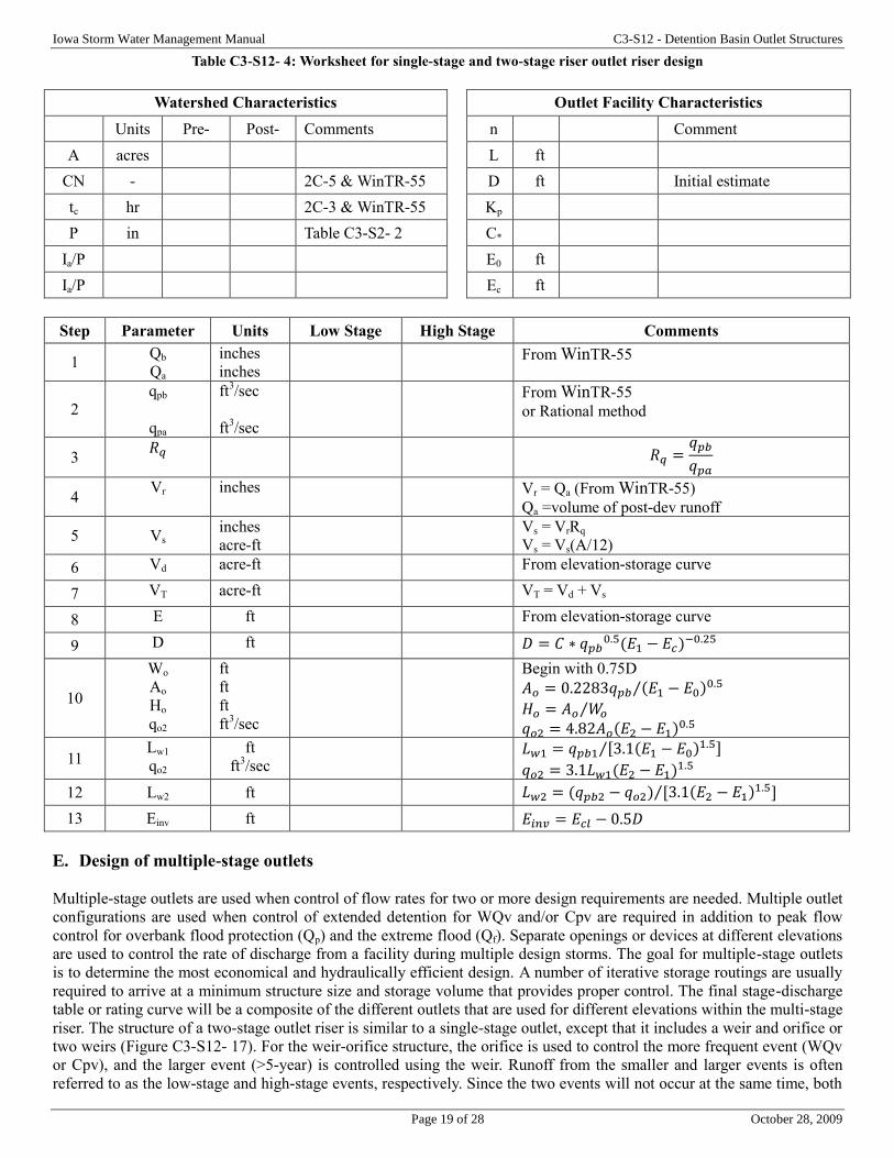
Iowa Storm Water Management Manual C3-S12 - Detention Basin Outlet Structures
Page 19 of 28 October 28, 2009
Table C3-S12- 4: Worksheet for single-stage and two-stage riser outlet riser design
Watershed Characteristics Outlet Facility Characteristics
Units Pre- Post- Comments n Comment
A acres L ft
CN - 2C-5 & WinTR-55 D ft Initial estimate
tc hr 2C-3 & WinTR-55 Kp
P in Table C3-S2- 2 C*
Ia/P E0 ft
Ia/P Ec ft
Step Parameter Units Low Stage High Stage Comments
1 Qb
Qa
inches
inches
From WinTR-55
2
qpb
qpa
ft3/sec
ft3/sec
From WinTR-55
or Rational method
3 𝑅𝑞
𝑅𝑞 =𝑞𝑝𝑏
𝑞𝑝𝑎
4 Vr inches Vr = Qa (From WinTR-55)
Qa =volume of post-dev runoff
5 Vs inches
acre-ft
Vs = VrRq
Vs = Vs(A/12)
6 Vd acre-ft From elevation-storage curve
7 VT acre-ft VT = Vd + Vs
8 E ft From elevation-storage curve
9 D ft 𝐷 = 𝐶 ∗ 𝑞𝑝𝑏0.5(𝐸1 − 𝐸𝑐)−0.25
10
Wo
Ao
Ho
qo2
ft
ft
ft
ft3/sec
Begin with 0.75D
𝐴𝑜 = 0.2283𝑞𝑝𝑏 (𝐸1 − 𝐸0)0.5⁄
𝐻𝑜 = 𝐴𝑜 𝑊𝑜⁄
𝑞𝑜2 = 4.82𝐴𝑜(𝐸2 − 𝐸1)0.5
11 Lw1
qo2
ft
ft3/sec
𝐿𝑤1 = 𝑞𝑝𝑏1 [3.1(𝐸1 − 𝐸0)1.5]⁄
𝑞𝑜2 = 3.1𝐿𝑤1(𝐸2 − 𝐸1)1.5
12 Lw2 ft 𝐿𝑤2 = (𝑞𝑝𝑏2 − 𝑞𝑜2) [3.1(𝐸2 − 𝐸1)1.5]⁄
13 Einv ft 𝐸𝑖𝑛𝑣 = 𝐸𝑐𝑙 − 0.5𝐷
E. Design of multiple-stage outlets
Multiple-stage outlets are used when control of flow rates for two or more design requirements are needed. Multiple outlet
configurations are used when control of extended detention for WQv and/or Cpv are required in addition to peak flow
control for overbank flood protection (Qp) and the extreme flood (Qf). Separate openings or devices at different elevations
are used to control the rate of discharge from a facility during multiple design storms. The goal for multiple-stage outlets
is to determine the most economical and hydraulically efficient design. A number of iterative storage routings are usually
required to arrive at a minimum structure size and storage volume that provides proper control. The final stage-discharge
table or rating curve will be a composite of the different outlets that are used for different elevations within the multi-stage
riser. The structure of a two-stage outlet riser is similar to a single-stage outlet, except that it includes a weir and orifice or
two weirs (Figure C3-S12- 17). For the weir-orifice structure, the orifice is used to control the more frequent event (WQv
or Cpv), and the larger event (>5-year) is controlled using the weir. Runoff from the smaller and larger events is often
referred to as the low-stage and high-stage events, respectively. Since the two events will not occur at the same time, both
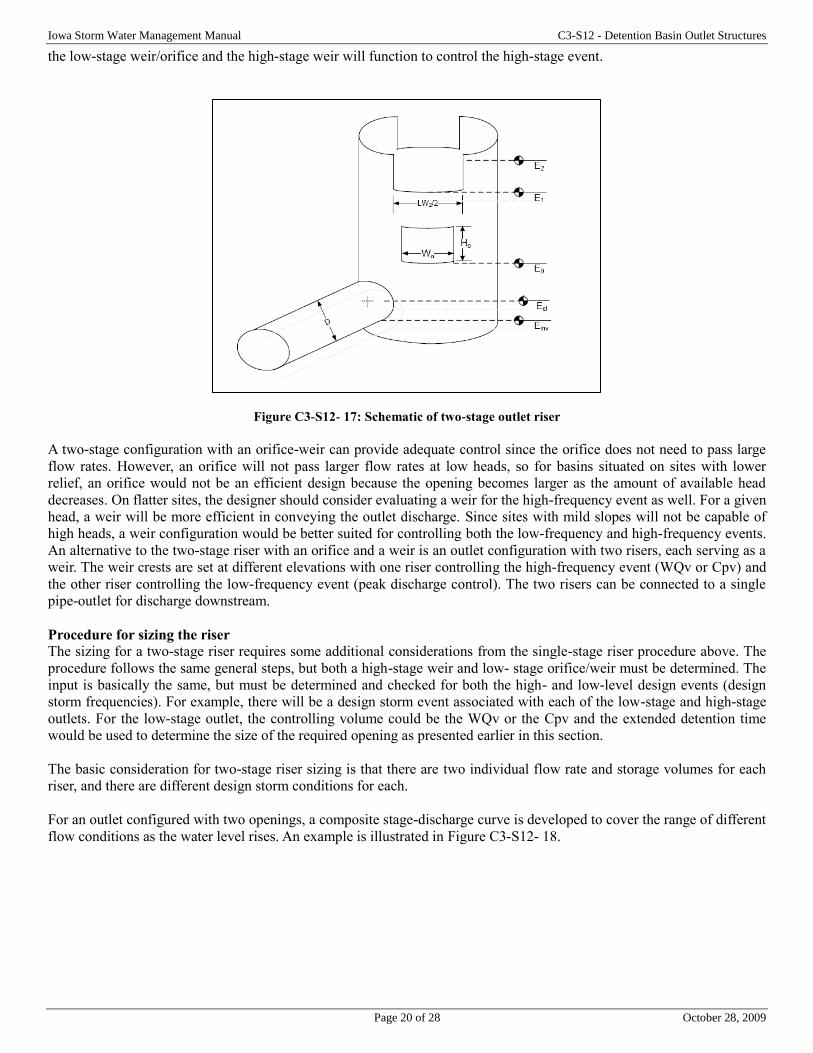
Iowa Storm Water Management Manual C3-S12 - Detention Basin Outlet Structures
Page 20 of 28 October 28, 2009
the low-stage weir/orifice and the high-stage weir will function to control the high-stage event.
Figure C3-S12- 17: Schematic of two-stage outlet riser
A two-stage configuration with an orifice-weir can provide adequate control since the orifice does not need to pass large
flow rates. However, an orifice will not pass larger flow rates at low heads, so for basins situated on sites with lower
relief, an orifice would not be an efficient design because the opening becomes larger as the amount of available head
decreases. On flatter sites, the designer should consider evaluating a weir for the high-frequency event as well. For a given
head, a weir will be more efficient in conveying the outlet discharge. Since sites with mild slopes will not be capable of
high heads, a weir configuration would be better suited for controlling both the low-frequency and high-frequency events.
An alternative to the two-stage riser with an orifice and a weir is an outlet configuration with two risers, each serving as a
weir. The weir crests are set at different elevations with one riser controlling the high-frequency event (WQv or Cpv) and
the other riser controlling the low-frequency event (peak discharge control). The two risers can be connected to a single
pipe-outlet for discharge downstream.
Procedure for sizing the riser
The sizing for a two-stage riser requires some additional considerations from the single-stage riser procedure above. The
procedure follows the same general steps, but both a high-stage weir and low- stage orifice/weir must be determined. The
input is basically the same, but must be determined and checked for both the high- and low-level design events (design
storm frequencies). For example, there will be a design storm event associated with each of the low-stage and high-stage
outlets. For the low-stage outlet, the controlling volume could be the WQv or the Cpv and the extended detention time
would be used to determine the size of the required opening as presented earlier in this section.
The basic consideration for two-stage riser sizing is that there are two individual flow rate and storage volumes for each
riser, and there are different design storm conditions for each.
For an outlet configured with two openings, a composite stage-discharge curve is developed to cover the range of different
flow conditions as the water level rises. An example is illustrated in Figure C3-S12- 18.
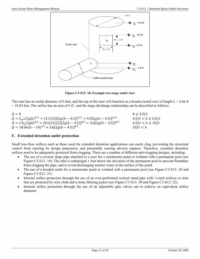
Iowa Storm Water Management Manual C3-S12 - Detention Basin Outlet Structures
Page 21 of 28 October 28, 2009
Figure C3-S12- 18: Example two-stage outlet riser
The riser has an inside diameter of 6 feet, and the top of the riser will function as a broad-crested weir of length L = 6.0π ft
= 18.84 feet. The orifice has an area of 6 ft2, and the stage-discharge relationship can be described as follows:
𝑄 = 0 ℎ ≤ 4.5𝑓𝑡
𝑄 = 𝐶𝑤𝐿(2𝑔ℎ)3 2⁄ = (3.1)(3)[2𝑔(ℎ − 4.5)]3 2⁄ = 9.3[2𝑔(ℎ − 4.5)]3 2⁄ 4.5𝑓𝑡 < ℎ ≤ 6.5𝑓𝑡
𝑄 = 𝐶𝐴𝑜(2𝑔ℎ)0.5 = (0.6)(3)(2)[2𝑔(ℎ − 4.5)]0.5 = 3.6[2𝑔(ℎ − 4.5)]0.5 6.5𝑓𝑡 < ℎ ≤ 10𝑓𝑡
𝑄 = 18.0𝜋(ℎ − 10)1.5 + 3.6[2𝑔(ℎ − 4.5)]0.5 10𝑓𝑡 < ℎ
F. Extended detention outlet protection
Small low-flow orifices such as those used for extended detention applications can easily clog, preventing the structural
control from meeting its design purpose(s), and potentially causing adverse impacts. Therefore, extended detention
orifices need to be adequately protected from clogging. There are a number of different anti-clogging designs, including:
The use of a reverse slope pipe attached to a riser for a stormwater pond or wetland with a permanent pool (see
Figure C3-S12- 19). The inlet is submerged 1 foot below the elevation of the permanent pool to prevent floatables
from clogging the pipe, and to avoid discharging warmer water at the surface of the pond.
The use of a hooded outlet for a stormwater pond or wetland with a permanent pool (see Figure C3-S12- 20 and
Figure C3-S12- 21).
Internal orifice protection through the use of an over-perforated vertical stand pipe with ½-inch orifices or slots
that are protected by wire cloth and a stone filtering jacket (see Figure C3-S12- 20 and Figure C3-S12- 22).
Internal orifice protection through the use of an adjustable gate valves can to achieve an equivalent orifice
diameter.
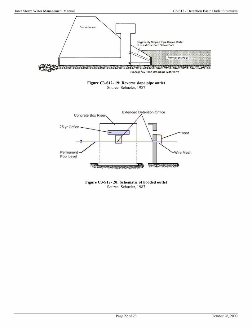
Iowa Storm Water Management Manual C3-S12 - Detention Basin Outlet Structures
Page 22 of 28 October 28, 2009
Figure C3-S12- 19: Reverse slope pipe outlet
Source: Schueler, 1987
Figure C3-S12- 20: Schematic of hooded outlet
Source: Schueler, 1987
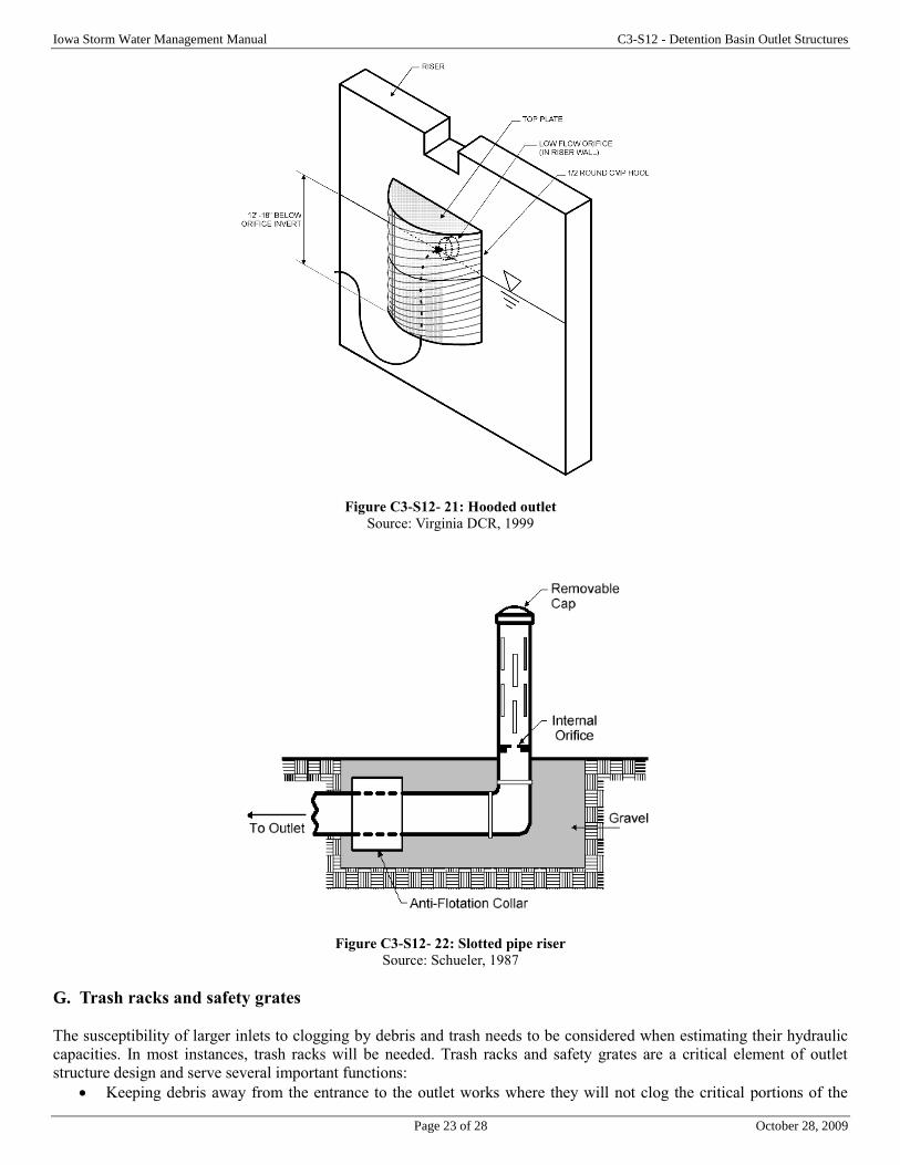
Iowa Storm Water Management Manual C3-S12 - Detention Basin Outlet Structures
Page 23 of 28 October 28, 2009
Figure C3-S12- 21: Hooded outlet
Source: Virginia DCR, 1999
Figure C3-S12- 22: Slotted pipe riser
Source: Schueler, 1987
G. Trash racks and safety grates
The susceptibility of larger inlets to clogging by debris and trash needs to be considered when estimating their hydraulic
capacities. In most instances, trash racks will be needed. Trash racks and safety grates are a critical element of outlet
structure design and serve several important functions:
Keeping debris away from the entrance to the outlet works where they will not clog the critical portions of the
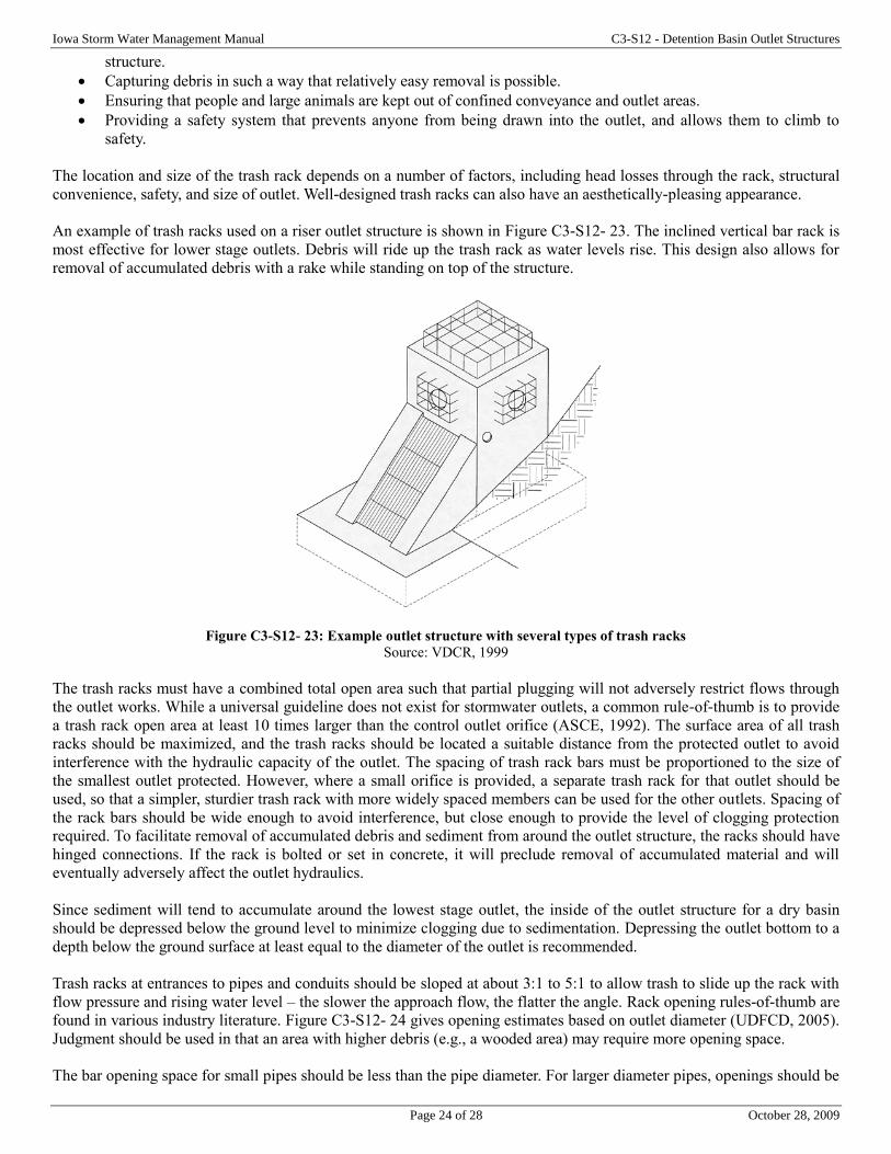
Iowa Storm Water Management Manual C3-S12 - Detention Basin Outlet Structures
Page 24 of 28 October 28, 2009
structure.
Capturing debris in such a way that relatively easy removal is possible.
Ensuring that people and large animals are kept out of confined conveyance and outlet areas.
Providing a safety system that prevents anyone from being drawn into the outlet, and allows them to climb to
safety.
The location and size of the trash rack depends on a number of factors, including head losses through the rack, structural
convenience, safety, and size of outlet. Well-designed trash racks can also have an aesthetically-pleasing appearance.
An example of trash racks used on a riser outlet structure is shown in Figure C3-S12- 23. The inclined vertical bar rack is
most effective for lower stage outlets. Debris will ride up the trash rack as water levels rise. This design also allows for
removal of accumulated debris with a rake while standing on top of the structure.
Figure C3-S12- 23: Example outlet structure with several types of trash racks
Source: VDCR, 1999
The trash racks must have a combined total open area such that partial plugging will not adversely restrict flows through
the outlet works. While a universal guideline does not exist for stormwater outlets, a common rule-of-thumb is to provide
a trash rack open area at least 10 times larger than the control outlet orifice (ASCE, 1992). The surface area of all trash
racks should be maximized, and the trash racks should be located a suitable distance from the protected outlet to avoid
interference with the hydraulic capacity of the outlet. The spacing of trash rack bars must be proportioned to the size of
the smallest outlet protected. However, where a small orifice is provided, a separate trash rack for that outlet should be
used, so that a simpler, sturdier trash rack with more widely spaced members can be used for the other outlets. Spacing of
the rack bars should be wide enough to avoid interference, but close enough to provide the level of clogging protection
required. To facilitate removal of accumulated debris and sediment from around the outlet structure, the racks should have
hinged connections. If the rack is bolted or set in concrete, it will preclude removal of accumulated material and will
eventually adversely affect the outlet hydraulics.
Since sediment will tend to accumulate around the lowest stage outlet, the inside of the outlet structure for a dry basin
should be depressed below the ground level to minimize clogging due to sedimentation. Depressing the outlet bottom to a
depth below the ground surface at least equal to the diameter of the outlet is recommended.
Trash racks at entrances to pipes and conduits should be sloped at about 3:1 to 5:1 to allow trash to slide up the rack with
flow pressure and rising water level – the slower the approach flow, the flatter the angle. Rack opening rules-of-thumb are
found in various industry literature. Figure C3-S12- 24 gives opening estimates based on outlet diameter (UDFCD, 2005).
Judgment should be used in that an area with higher debris (e.g., a wooded area) may require more opening space.
The bar opening space for small pipes should be less than the pipe diameter. For larger diameter pipes, openings should be
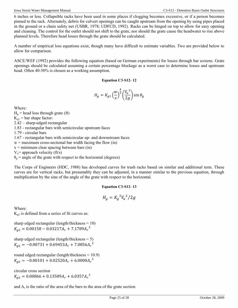
Iowa Storm Water Management Manual C3-S12 - Detention Basin Outlet Structures
Page 25 of 28 October 28, 2009
6 inches or less. Collapsible racks have been used in some places if clogging becomes excessive, or if a person becomes
pinned to the rack. Alternately, debris for culvert openings can be caught upstream from the opening by using pipes placed
in the ground or a chain safety net (USBR, 1978; UDFCD, 1992). Racks can be hinged on top to allow for easy opening
and cleaning. The control for the outlet should not shift to the grate, nor should the grate cause the headwater to rise above
planned levels. Therefore head losses through the grate should be calculated.
A number of empirical loss equations exist, though many have difficult to estimate variables. Two are provided below to
allow for comparison.
ASCE/WEF (1992) provides the following equation (based on German experiments) for losses through bar screens. Grate
openings should be calculated assuming a certain percentage blockage as a worst case to determine losses and upstream
head. Often 40-50% is chosen as a working assumption.
Equation C3-S12- 12
𝐻𝑔 = 𝐾𝑔1 (𝑤
𝑥)
43
(𝑉𝑢
2
2𝑔) sin 𝜃𝑔
Where:
Hg = head loss through grate (ft)
Kg1 = bar shape factor:
2.42 – sharp-edged rectangular
1.83 - rectangular bars with semicircular upstream faces
1.79 - circular bars
1.67 - rectangular bars with semicircular up- and downstream faces
w = maximum cross-sectional bar width facing the flow (in)
x = minimum clear spacing between bars (in)
Vu= approach velocity (ft/s)
θg = angle of the grate with respect to the horizontal (degrees)
The Corps of Engineers (HDC, 1988) has developed curves for trash racks based on similar and additional tests. These
curves are for vertical racks, but presumably they can be adjusted, in a manner similar to the previous equation, through
multiplication by the sine of the angle of the grate with respect to the horizontal.
Equation C3-S12- 13
𝐻𝑔 = 𝐾𝑔2𝑉𝑢
2 2𝑔⁄
Where:
Kg2 is defined from a series of fit curves as:
sharp edged rectangular (length/thickness = 10)
𝐾𝑔2 = 0.00158 − 0.03217𝐴𝑟 + 7.1789𝐴𝑟2
sharp edged rectangular (length/thickness = 5)
𝐾𝑔2 = −0.00731 + 0.69453𝐴𝑟 + 7.0856𝐴𝑟2
round edged rectangular (length/thickness = 10.9)
𝐾𝑔2 = −0.00101 + 0.02520𝐴𝑟 + 6.0000𝐴𝑟2
circular cross section
𝐾𝑔2 = 0.00866 + 0.13589𝐴𝑟 + 6.0357𝐴𝑟2
and Ar is the ratio of the area of the bars to the area of the grate section.
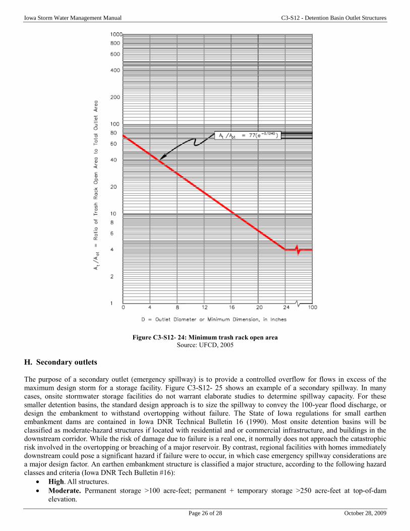
Iowa Storm Water Management Manual C3-S12 - Detention Basin Outlet Structures
Page 26 of 28 October 28, 2009
Figure C3-S12- 24: Minimum trash rack open area
Source: UFCD, 2005
H. Secondary outlets
The purpose of a secondary outlet (emergency spillway) is to provide a controlled overflow for flows in excess of the
maximum design storm for a storage facility. Figure C3-S12- 25 shows an example of a secondary spillway. In many
cases, onsite stormwater storage facilities do not warrant elaborate studies to determine spillway capacity. For these
smaller detention basins, the standard design approach is to size the spillway to convey the 100-year flood discharge, or
design the embankment to withstand overtopping without failure. The State of Iowa regulations for small earthen
embankment dams are contained in Iowa DNR Technical Bulletin 16 (1990). Most onsite detention basins will be
classified as moderate-hazard structures if located with residential and or commercial infrastructure, and buildings in the
downstream corridor. While the risk of damage due to failure is a real one, it normally does not approach the catastrophic
risk involved in the overtopping or breaching of a major reservoir. By contrast, regional facilities with homes immediately
downstream could pose a significant hazard if failure were to occur, in which case emergency spillway considerations are
a major design factor. An earthen embankment structure is classified a major structure, according to the following hazard
classes and criteria (Iowa DNR Tech Bulletin #16):
High. All structures.
Moderate. Permanent storage >100 acre-feet; permanent + temporary storage >250 acre-feet at top-of-dam
elevation.

Iowa Storm Water Management Manual C3-S12 - Detention Basin Outlet Structures
Page 27 of 28 October 28, 2009
Low. Height-storage product >30,000 (based on emergency spillway crest elevation).
For moderate-hazard and low-hazard dams classified as major structures, the freeboard design flood is determined as:
0.5 x PMF (probable maximum flood)
Flood hydrograph produced by multiplying the ordinate of the PMF hydrograph by 0.5
6-hour duration storms
For low-hazard dams not classified as major structures the freeboard design flood is determined as:
Product of emergency spillway crest height in feet (measured from channel elevation at centerline of dam) and the
total storage volume (acre-ft) at the emergency spillway crest elevation is between 3,000 and 30,000
𝑅𝑎𝑖𝑛𝑓𝑎𝑙𝑙 = 𝑃100 + 0.12(𝑃𝑀𝑃 − 𝑃100)
6-hour storm duration
For dams without emergency spillways, storage volume and effective height determined by measuring from
channel bottom to top of dam at the centerline.
Rainfall = P50 and 24-hour duration event
Emergency spillway design
Emergency spillway designs are open channels, usually trapezoidal in cross section, and consist of an inlet channel, a
control section, and an exit channel (see Figure C3-S12- 25). The emergency spillway is proportioned to pass flows in
excess of the design flood (typically the 100-year flood or greater) without allowing excessive velocities, and without
overtopping of the embankment. Flow in the emergency spillway is open channel flow (see Chapter 15 for more
information). Normally, it is assumed that critical depth occurs at the control section. NRCS manuals provide guidance for
the selection of emergency spillway characteristics for different soil conditions and different types of vegetation. The
selection of degree of retardance for a given spillway depends on the vegetation. Knowing the retardance factor and the
estimated discharge rate, the emergency spillway bottom width can be determined. For erosion protection during the first
year, assume minimum retardance. Both the inlet and exit channels should have a straight alignment and grade. Spillway
side slopes should be no steeper than 3:1 horizontal to vertical.
General design criteria for secondary spillways are:
Should only operate at floods greater than the principal spillway design flood
Flow velocities should be non-erosive: ≈5 fps
Construct on undisturbed soil
Use ramp spillway on constructed fill
Use smooth horizontal and vertical transitions and alignments
Place outlet a safe distance from the downstream toe of the structure
Energy dissipation at the outlet
Design criteria for earthen secondary spillways are:
Minimum bottom width: 10 feet
For major structures, minimum depth is 3 feet
For non-major structures, minimum depth is 2 feet
Profile through the emergency spillway should be horizontal for at least 30 feet through the crest control section
Exit channel slopes: >1% and <10%; maintain critical depth control at the crest
The most common type of emergency spillway used is a broad-crested overflow weir cut through original ground next to
the embankment. The transverse cross section of the weir cut is typically trapezoidal in shape for ease of construction.
Such an excavated emergency spillway is illustrated below.
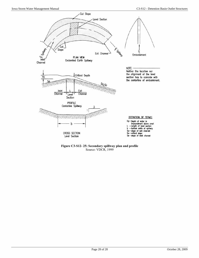
Iowa Storm Water Management Manual C3-S12 - Detention Basin Outlet Structures
Page 28 of 28 October 28, 2009
Figure C3-S12- 25: Secondary spillway plan and profile
Source: VDCR, 1999
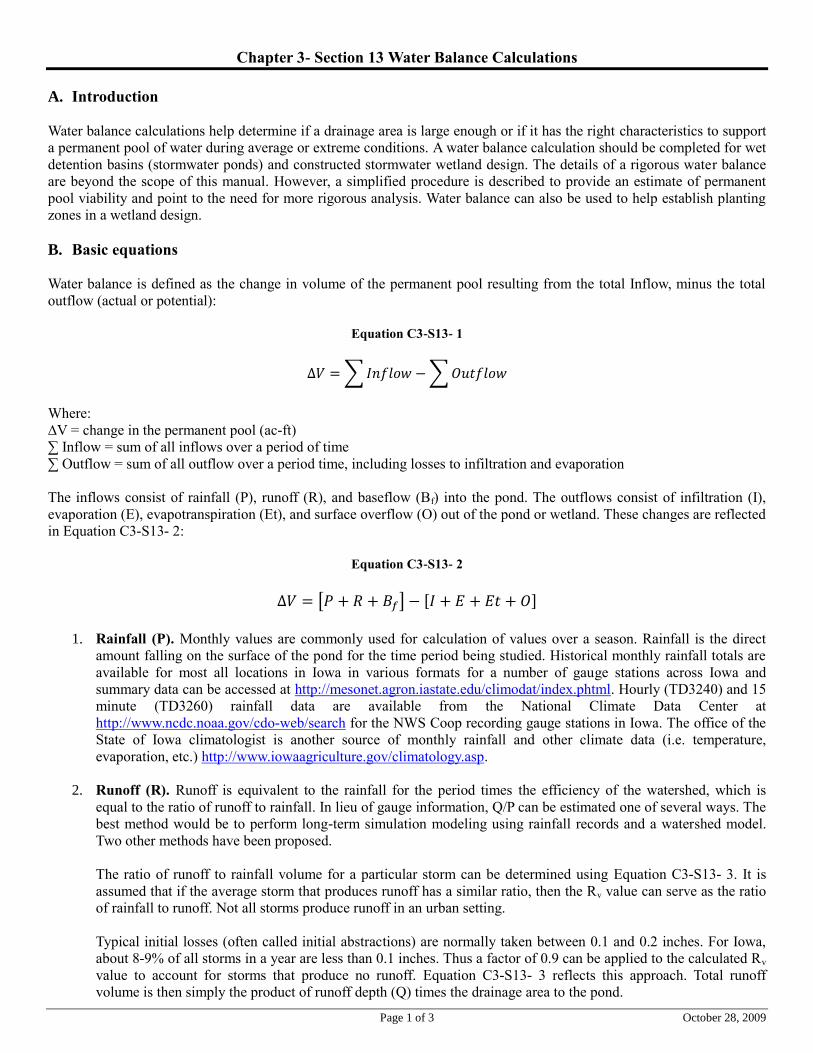
Page 1 of 3 October 28, 2009
Chapter 3- Section 13 Water Balance Calculations
A. Introduction
Water balance calculations help determine if a drainage area is large enough or if it has the right characteristics to support
a permanent pool of water during average or extreme conditions. A water balance calculation should be completed for wet
detention basins (stormwater ponds) and constructed stormwater wetland design. The details of a rigorous water balance
are beyond the scope of this manual. However, a simplified procedure is described to provide an estimate of permanent
pool viability and point to the need for more rigorous analysis. Water balance can also be used to help establish planting
zones in a wetland design.
B. Basic equations
Water balance is defined as the change in volume of the permanent pool resulting from the total Inflow, minus the total
outflow (actual or potential):
Equation C3-S13- 1
∆𝑉 = ∑ 𝐼𝑛𝑓𝑙𝑜𝑤 − ∑ 𝑂𝑢𝑡𝑓𝑙𝑜𝑤
Where:
∆V = change in the permanent pool (ac-ft)
∑ Inflow = sum of all inflows over a period of time
∑ Outflow = sum of all outflow over a period time, including losses to infiltration and evaporation
The inflows consist of rainfall (P), runoff (R), and baseflow (Bf) into the pond. The outflows consist of infiltration (I),
evaporation (E), evapotranspiration (Et), and surface overflow (O) out of the pond or wetland. These changes are reflected
in Equation C3-S13- 2:
Equation C3-S13- 2
∆𝑉 = [𝑃 + 𝑅 + 𝐵𝑓] − [𝐼 + 𝐸 + 𝐸𝑡 + 𝑂]
1. Rainfall (P). Monthly values are commonly used for calculation of values over a season. Rainfall is the direct
amount falling on the surface of the pond for the time period being studied. Historical monthly rainfall totals are
available for most all locations in Iowa in various formats for a number of gauge stations across Iowa and
summary data can be accessed at http://mesonet.agron.iastate.edu/climodat/index.phtml. Hourly (TD3240) and 15
minute (TD3260) rainfall data are available from the National Climate Data Center at
http://www.ncdc.noaa.gov/cdo-web/search for the NWS Coop recording gauge stations in Iowa. The office of the
State of Iowa climatologist is another source of monthly rainfall and other climate data (i.e. temperature,
evaporation, etc.) http://www.iowaagriculture.gov/climatology.asp.
2. Runoff (R). Runoff is equivalent to the rainfall for the period times the efficiency of the watershed, which is
equal to the ratio of runoff to rainfall. In lieu of gauge information, Q/P can be estimated one of several ways. The
best method would be to perform long-term simulation modeling using rainfall records and a watershed model.
Two other methods have been proposed.
The ratio of runoff to rainfall volume for a particular storm can be determined using Equation C3-S13- 3. It is
assumed that if the average storm that produces runoff has a similar ratio, then the Rv value can serve as the ratio
of rainfall to runoff. Not all storms produce runoff in an urban setting.
Typical initial losses (often called initial abstractions) are normally taken between 0.1 and 0.2 inches. For Iowa,
about 8-9% of all storms in a year are less than 0.1 inches. Thus a factor of 0.9 can be applied to the calculated Rv
value to account for storms that produce no runoff. Equation C3-S13- 3 reflects this approach. Total runoff
volume is then simply the product of runoff depth (Q) times the drainage area to the pond.
Iowa Storm Water Management Manual C3-S13 - Water Balance Calculations
Page 2 of 3 October 28, 2009
Equation C3-S13- 3
𝑄 = 0.9𝑃𝑅𝑣
Where:
P = precipitation (in)
Q = runoff volume (in)
Rv = volumetric runoff coefficient for the watershed
The WinTR-55 program can be used to model a range of storms using the CN method to predict the individual
storm runoff. These values can be plotted by rainfall depth and applied to monthly rainfall to create a monthly
runoff model.
Most stormwater ponds and wetlands have little, if any, baseflow, as they are rarely placed across perennial
streams. If so placed, baseflow must be estimated from observation or through theoretical estimates. Methods of
estimation and baseflow separation can be found in most hydrology textbooks.
3. Infiltration (I). Infiltration is a very complex subject and cannot be covered in detail here. More detailed
information is included in Chapter 5, including data on nominal infiltration rates and soil water capacity. The
amount of infiltration depends on soils, water table depth, rock layers, surface disturbance, the presence or
absence of a liner in the pond, and other factors. The infiltration rate is governed by the Darcy equation as:
Equation C3-S13- 4
𝐼 = 𝐴𝐾ℎ𝐺ℎ
Where:
I = infiltration (ac-ft/day)
A = cross-sectional area through which the water infiltrates (ac)
Kh = saturated hydraulic conductivity or infiltration rate (ft/day)
Gh = hydraulic gradient = pressure head/distance
Gh can be set equal to 1.0 for pond bottoms and 0.5 for pond sides steeper than about 4:1. Infiltration rate can be
established through testing, though not always accurately.
4. Evaporation (E). Evaporation is from an open lake water surface. Evaporation rates are dependent on differences
in vapor pressure, which in turn depend on temperature, wind, atmospheric pressure, water purity, and shape and
depth of the pond. It is estimated or measured in a number of ways, which can be found in most hydrology
textbooks. Monthly evaporation data for Iowa is available from the National Climate Data Center (NCDC) at
http://www.ncdc.noaa.gov/cdo-web/search. In Iowa, evaporation data is reported as monthly averages for May
through September, and as 10-day averages for the last days of April and first days of October. Evaporation data is
not recorded between October 11 and April 20, due to sub- freezing weather conditions.
5. Evapotranspiration (Et). Evapotranspiration consists of the combination of evaporation and transpiration by
plants. The estimation of Et for crops in Iowa is well-documented and has become standard practice. However, for
wetlands, the estimating methods are not documented, nor are there consistent studies to assist the designer in
estimating the demand wetland plants would put on water volumes. Estimating Et only becomes important when
wetlands are being designed, and emergent vegetation covers a significant portion of the pond surface. In these
cases, conservative estimates of lake evaporation should be compared to crop-based Et estimates, and a decision
made. Crop-based Et estimates can be obtained from typical hydrology textbooks or from the websites mentioned
above. The climate website at Iowa State University in the Department of Agronomy can provide additional
information: http://mesonet.agron.iastate.edu/climodat/index.phtml.
6. Overflow (O). Overflow is considered as excess runoff. In water balance design, overflow is either not
considered, since the concern is for average values of precipitation; or is considered lost for all volumes above the

Iowa Storm Water Management Manual C3-S13 - Water Balance Calculations
Page 3 of 3 October 28, 2009
maximum pond storage. Obviously, for long-term simulations of rainfall runoff, large storms would play an
important part in pond design.
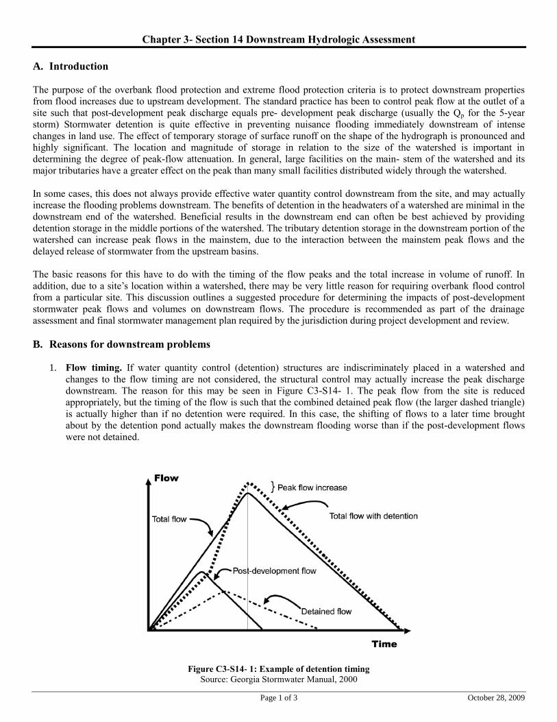
Page 1 of 3 October 28, 2009
Chapter 3- Section 14 Downstream Hydrologic Assessment
A. Introduction
The purpose of the overbank flood protection and extreme flood protection criteria is to protect downstream properties
from flood increases due to upstream development. The standard practice has been to control peak flow at the outlet of a
site such that post-development peak discharge equals pre- development peak discharge (usually the Qp for the 5-year
storm) Stormwater detention is quite effective in preventing nuisance flooding immediately downstream of intense
changes in land use. The effect of temporary storage of surface runoff on the shape of the hydrograph is pronounced and
highly significant. The location and magnitude of storage in relation to the size of the watershed is important in
determining the degree of peak-flow attenuation. In general, large facilities on the main- stem of the watershed and its
major tributaries have a greater effect on the peak than many small facilities distributed widely through the watershed.
In some cases, this does not always provide effective water quantity control downstream from the site, and may actually
increase the flooding problems downstream. The benefits of detention in the headwaters of a watershed are minimal in the
downstream end of the watershed. Beneficial results in the downstream end can often be best achieved by providing
detention storage in the middle portions of the watershed. The tributary detention storage in the downstream portion of the
watershed can increase peak flows in the mainstem, due to the interaction between the mainstem peak flows and the
delayed release of stormwater from the upstream basins.
The basic reasons for this have to do with the timing of the flow peaks and the total increase in volume of runoff. In
addition, due to a site’s location within a watershed, there may be very little reason for requiring overbank flood control
from a particular site. This discussion outlines a suggested procedure for determining the impacts of post-development
stormwater peak flows and volumes on downstream flows. The procedure is recommended as part of the drainage
assessment and final stormwater management plan required by the jurisdiction during project development and review.
B. Reasons for downstream problems
1. Flow timing. If water quantity control (detention) structures are indiscriminately placed in a watershed and
changes to the flow timing are not considered, the structural control may actually increase the peak discharge
downstream. The reason for this may be seen in Figure C3-S14- 1. The peak flow from the site is reduced
appropriately, but the timing of the flow is such that the combined detained peak flow (the larger dashed triangle)
is actually higher than if no detention were required. In this case, the shifting of flows to a later time brought
about by the detention pond actually makes the downstream flooding worse than if the post-development flows
were not detained.
Figure C3-S14- 1: Example of detention timing
Source: Georgia Stormwater Manual, 2000
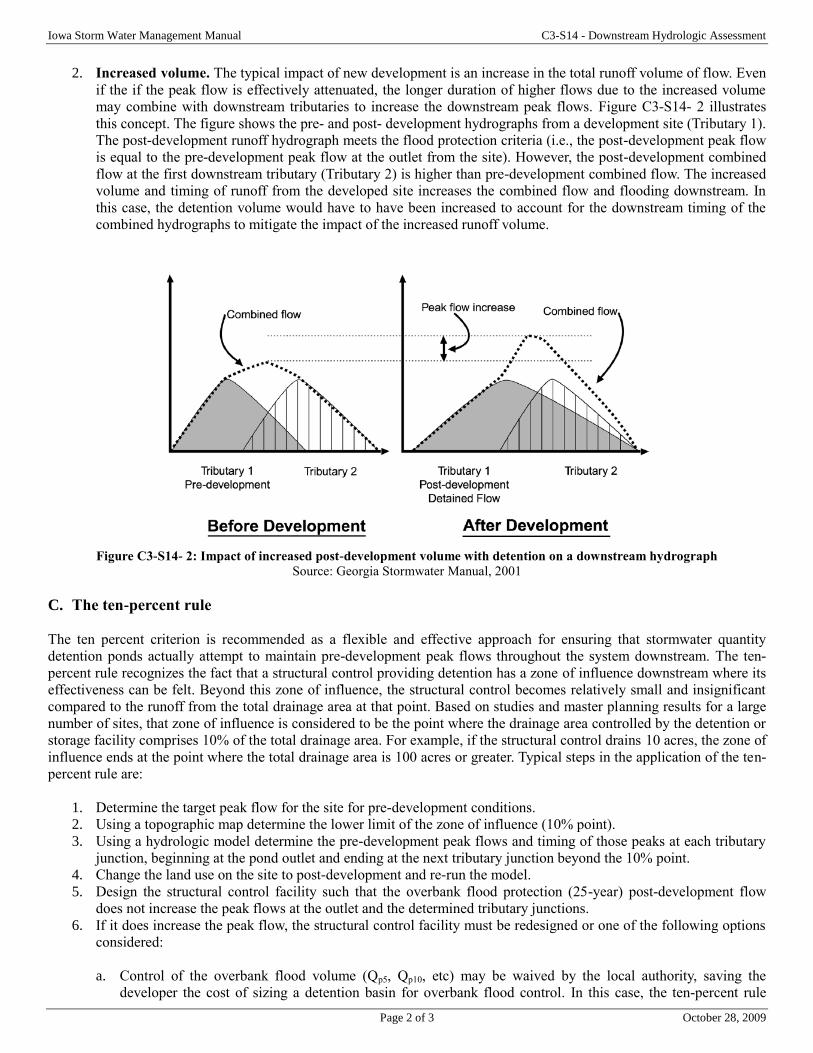
Iowa Storm Water Management Manual C3-S14 - Downstream Hydrologic Assessment
Page 2 of 3 October 28, 2009
2. Increased volume. The typical impact of new development is an increase in the total runoff volume of flow. Even
if the if the peak flow is effectively attenuated, the longer duration of higher flows due to the increased volume
may combine with downstream tributaries to increase the downstream peak flows. Figure C3-S14- 2 illustrates
this concept. The figure shows the pre- and post- development hydrographs from a development site (Tributary 1).
The post-development runoff hydrograph meets the flood protection criteria (i.e., the post-development peak flow
is equal to the pre-development peak flow at the outlet from the site). However, the post-development combined
flow at the first downstream tributary (Tributary 2) is higher than pre-development combined flow. The increased
volume and timing of runoff from the developed site increases the combined flow and flooding downstream. In
this case, the detention volume would have to have been increased to account for the downstream timing of the
combined hydrographs to mitigate the impact of the increased runoff volume.
Figure C3-S14- 2: Impact of increased post-development volume with detention on a downstream hydrograph
Source: Georgia Stormwater Manual, 2001
C. The ten-percent rule
The ten percent criterion is recommended as a flexible and effective approach for ensuring that stormwater quantity
detention ponds actually attempt to maintain pre-development peak flows throughout the system downstream. The ten-
percent rule recognizes the fact that a structural control providing detention has a zone of influence downstream where its
effectiveness can be felt. Beyond this zone of influence, the structural control becomes relatively small and insignificant
compared to the runoff from the total drainage area at that point. Based on studies and master planning results for a large
number of sites, that zone of influence is considered to be the point where the drainage area controlled by the detention or
storage facility comprises 10% of the total drainage area. For example, if the structural control drains 10 acres, the zone of
influence ends at the point where the total drainage area is 100 acres or greater. Typical steps in the application of the ten-
percent rule are:
1. Determine the target peak flow for the site for pre-development conditions.
2. Using a topographic map determine the lower limit of the zone of influence (10% point).
3. Using a hydrologic model determine the pre-development peak flows and timing of those peaks at each tributary
junction, beginning at the pond outlet and ending at the next tributary junction beyond the 10% point.
4. Change the land use on the site to post-development and re-run the model.
5. Design the structural control facility such that the overbank flood protection (25-year) post-development flow
does not increase the peak flows at the outlet and the determined tributary junctions.
6. If it does increase the peak flow, the structural control facility must be redesigned or one of the following options
considered:
a. Control of the overbank flood volume (Qp5, Qp10, etc) may be waived by the local authority, saving the
developer the cost of sizing a detention basin for overbank flood control. In this case, the ten-percent rule
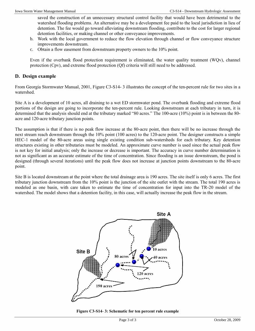
Iowa Storm Water Management Manual C3-S14 - Downstream Hydrologic Assessment
Page 3 of 3 October 28, 2009
saved the construction of an unnecessary structural control facility that would have been detrimental to the
watershed flooding problems. An alternative may be a development fee paid to the local jurisdiction in lieu of
detention. The fee would go toward alleviating downstream flooding, contribute to the cost for larger regional
detention facilities, or making channel or other conveyance improvements.
b. Work with the local government to reduce the flow elevation through channel or flow conveyance structure
improvements downstream.
c. Obtain a flow easement from downstream property owners to the 10% point.
Even if the overbank flood protection requirement is eliminated, the water quality treatment (WQv), channel
protection (Cpv), and extreme flood protection (Qf) criteria will still need to be addressed.
D. Design example
From Georgia Stormwater Manual, 2001, Figure C3-S14- 3 illustrates the concept of the ten-percent rule for two sites in a
watershed.
Site A is a development of 10 acres, all draining to a wet ED stormwater pond. The overbank flooding and extreme flood
portions of the design are going to incorporate the ten-percent rule. Looking downstream at each tributary in turn, it is
determined that the analysis should end at the tributary marked “80 acres.” The 100-acre (10%) point is in between the 80-
acre and 120-acre tributary junction points.
The assumption is that if there is no peak flow increase at the 80-acre point, then there will be no increase through the
next stream reach downstream through the 10% point (100 acres) to the 120-acre point. The designer constructs a simple
HEC-1 model of the 80-acre areas using single existing condition sub-watersheds for each tributary. Key detention
structures existing in other tributaries must be modeled. An approximate curve number is used since the actual peak flow
is not key for initial analysis; only the increase or decrease is important. The accuracy in curve number determination is
not as significant as an accurate estimate of the time of concentration. Since flooding is an issue downstream, the pond is
designed (through several iterations) until the peak flow does not increase at junction points downstream to the 80-acre
point.
Site B is located downstream at the point where the total drainage area is 190 acres. The site itself is only 6 acres. The first
tributary junction downstream from the 10% point is the junction of the site outlet with the stream. The total 190 acres is
modeled as one basin, with care taken to estimate the time of concentration for input into the TR-20 model of the
watershed. The model shows that a detention facility, in this case, will actually increase the peak flow in the stream.
Figure C3-S14- 3: Schematic for ten percent rule example
Related Documents