Chapter 3. Magnetostatics ( ) - UWO Physics

58

Chapter 3. Magnetostatics Notes: • Most of the material presented in this chapter is taken from Jackson, Chap. 5.

3.1 Introduction Just as the electric field vector E is the basic quantity in electrostatics, the magnetic-flux density or magnetic induction B plays a fundamental role in magnetostatics. Another fundamental quantity is the magnetic dipole µ , which plays a role not unlike the electric charge in electrostatics. It is, however important to realize that, as far as we know, there does not exist any magnetic monopoles (or charges). The two quantities, B and µ , were early on linked through simple relations. For example, the torque N exerted by a magnetic-flux density on a test dipole (i.e., small enough not to alter the magnetic-flux) is given by N = µ ! B. (3.1) It was also established that there is a connection between electrical currents and magnetic fields. As will soon be shown, a current density J (or simply a current I ) is a source of magnetic-flux density. Since the current density is defined as the amount of charge that flows through a cross-section per unit of time (units of Coulombs per square meter-second), the conservation of charge requires that the so-called continuity equation be satisfied

!"

!t+# $ J = 0 (3.2)

Equation (3.2) implies that any decrease (increase) in charge density within a small volume must be accompanied by a corresponding flow of charges out of (in) the surface delimiting the volume. Because magnetostatics is concerned with steady-state currents, we will limit ourselves (at least in this chapter) to the following equation ! " J = 0. (3.3)

3.2 The Biot and Savart Law

The aforementioned link between the magnetic induction and the current, where the latter is a source for the former, was first investigated experimentally by Biot and Savart, and Ampère, and shown to be

dB =µ0

4!I dl " x( )

x3

= #µ0

4!I dl " $

1

x

%

&'(

)*, (3.4)

59

where µ0 is the permeability of vacuum (units of Henry per meter; µ

04! = 10

"7 H/m), dl is a small length element from a wire pointing in the direction of the current I , and x is the vector linking dl to the location where dB is evaluated (see Figure 3.1). It is apparent from equation (3.4) that dB is oriented perpendicular to the plane formed by dl and x . The lines of the magnetic induction are, therefore, concentric circles around the wire. Let’s consider, as an example, the case of an infinitely long wire carrying a current I . Integrating over the length of the wire, we find that

B =µ0

4!I

R dl

R2 + l2( )

3 2"#

#

$

=µ0

4!I

R

d%

cos2 %( ) 1+ tan2 %( )&' ()

3 2"! 2

! 2

$

=µ0

4!I

Rcos %( ) d%

"! 2

! 2

$

=µ0

2!I

R,

(3.5)

where we made the change of variable l = R tan !( ) . This result is known as the Biot and Savart Law. It was also determined experimentally that each of two current carrying wires experience a force due to the presence of the other. Since we know that a current produces a magnetic induction, this implies that there must exists a relation with the following form dF = I

1dl1! B( ). (3.6)

If B is due to another current I

2, we find the total force F

21 felt by the wire carrying I

1

using equation (3.4), with integrations around the two loops (or circuits) made by the wires (and x

12= x

1! x

2, see Figure 3.2)

Figure 3.1 – Magnetic induction dB from a current element I dl .

60

F21=µ0

4!I1I2

dl1" dl

2" x

12( )x12

3!#!#

=µ0

4!I1I2

dl2dl1$x

12( ) % dl1$dl

2( )x12&' ()

x12

3!#!# ,

(3.7)

since a ! b ! c( ) = a " c( )b # a "b( )c . The first term on the right-hand side of equation (3.7) can be shown to vanish, since

µ0

4!I1I2

dl2dl1"x

12( )x12

3!#!# =µ0

4!I1I2dl2

$2

1

x12

%

&'(

)*!#!# "dl1

= +µ0

4!I1I2dl2

$1

1

x12

%

&'(

)*!#!# "dl1

= +µ0

4!I1I2dl2

$1, $

1

1

x12

%

&'(

)*-

.//

0

122"n da#!#

= 0,

(3.8)

where we used Stokes’ theorem, and the fact that ! "! = 0. Equation (3.7) reduces to

F21= !

µ0

4"I1I2

dl1#dl

2( )x12$% &'x12

3!(!(

= !µ0

4"I1I2

dl1#dl

2( ))2

1

x12

*

+,-

./!(!( .

(3.9)

Figure 3.2 – The interaction between two current loops.

61

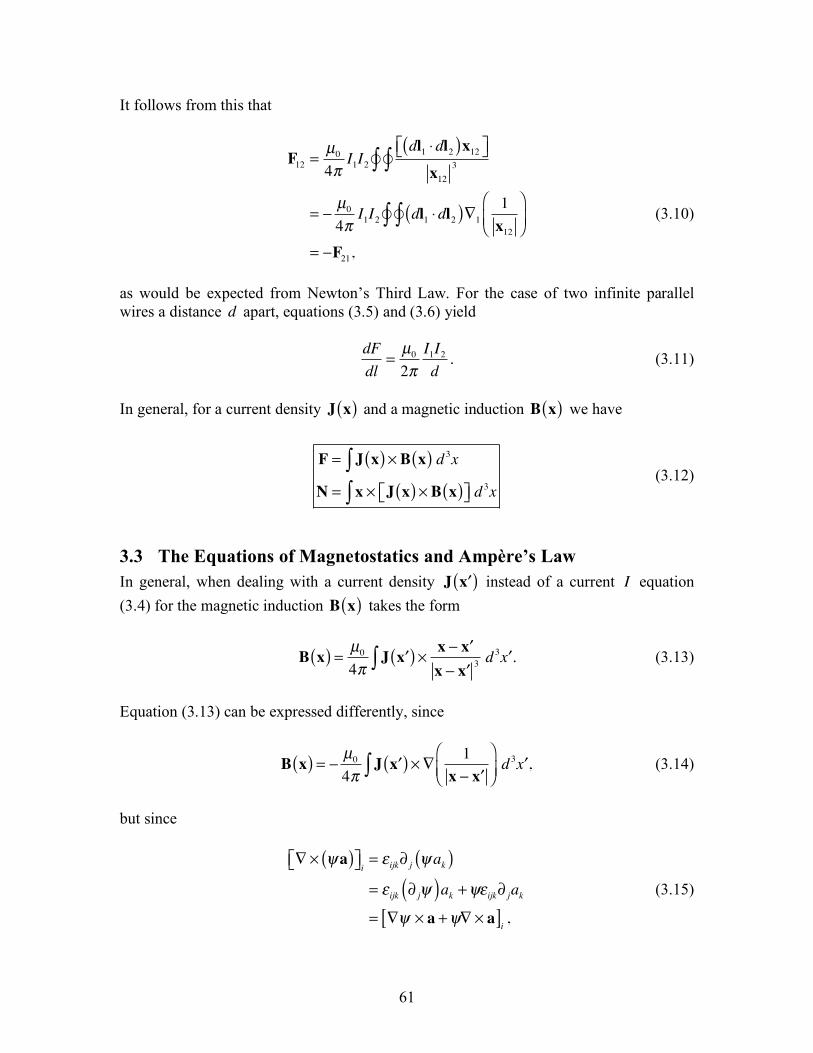
It follows from this that

F12=µ0

4!I1I2

dl1"dl

2( )x12#$ %&x12

3!'!'

= (µ0

4!I1I2

dl1"dl

2( ))1

1

x12

*

+,-

./!'!'= (F

21,

(3.10)

as would be expected from Newton’s Third Law. For the case of two infinite parallel wires a distance d apart, equations (3.5) and (3.6) yield

dF

dl=µ0

2!

I1I2

d. (3.11)

In general, for a current density J x( ) and a magnetic induction B x( ) we have

F = J x( ) ! B x( ) d 3x"N = x ! J x( ) ! B x( )#$ %& d

3x"

(3.12)

3.3 The Equations of Magnetostatics and Ampère’s Law In general, when dealing with a current density J !x( ) instead of a current I equation (3.4) for the magnetic induction B x( ) takes the form

B x( ) =µ0

4!J "x( ) #

x $ "x

x $ "x3% d

3 "x . (3.13)

Equation (3.13) can be expressed differently, since

B x( ) = !µ0

4"J #x( ) $ %

1

x ! #x

&

'()

*+, d3 #x , (3.14)

but since

! " #a( )$% &'i = (ijk) j #ak( )

= (ijk ) j#( )ak +#(ijk) jak

= !# " a +#! " a[ ]i,

(3.15)

62

we get

B x( ) =µ0

4!" #

J $x( )x % $x& d

3 $x , (3.16)

if we set ! = 1 x " #x and a = J #x( ) , with ! " J #x( ) = 0 , since the current density is independent of x . It follows from equation (3.16) that the magnetic induction is divergence-less ! "B = 0 (3.17) Equation (3.17) is a mathematical statement on the inexistence of magnetic monopoles. Taking the curl of the B field, remembering that ! " ! " a( ) = ! ! #a( ) $ !

2a , we get

! " B =µ0

4#! " ! "

J $x( )x % $x& d

3 $x'

()*

+,

=µ0

4#! J $x( ) -!

1

x % $x

'

()*

+,& d3 $x % J $x( )!2

1

x % $x

'

()*

+,& d3 $x

.

/00

1

233

(3.18)

and using equation (1.74)

! " B = #µ0

4$! J %x( ) & %!

1

x # %x

'

()*

+,- d3 %x + µ

0J x( ). (3.19)

This equation can be further simplified by using the divergence theorem

J !x( ) " !#1

x $ !x

%

&'(

)*+ d3 !x = !# "

J !x( )

x $ !x

%

&'(

)*+ d3 !x $

!# " J !x( )

x $ !x+ d3 !x

=J !x( )

x $ !x"n+ d !a

= 0,

(3.20)

since !" # J !x( ) = 0 (see equation (3.3)) and the surface of integration extends over all space where the integrand vanishes. We therefore find that ! " B = µ

0J (3.21)

63

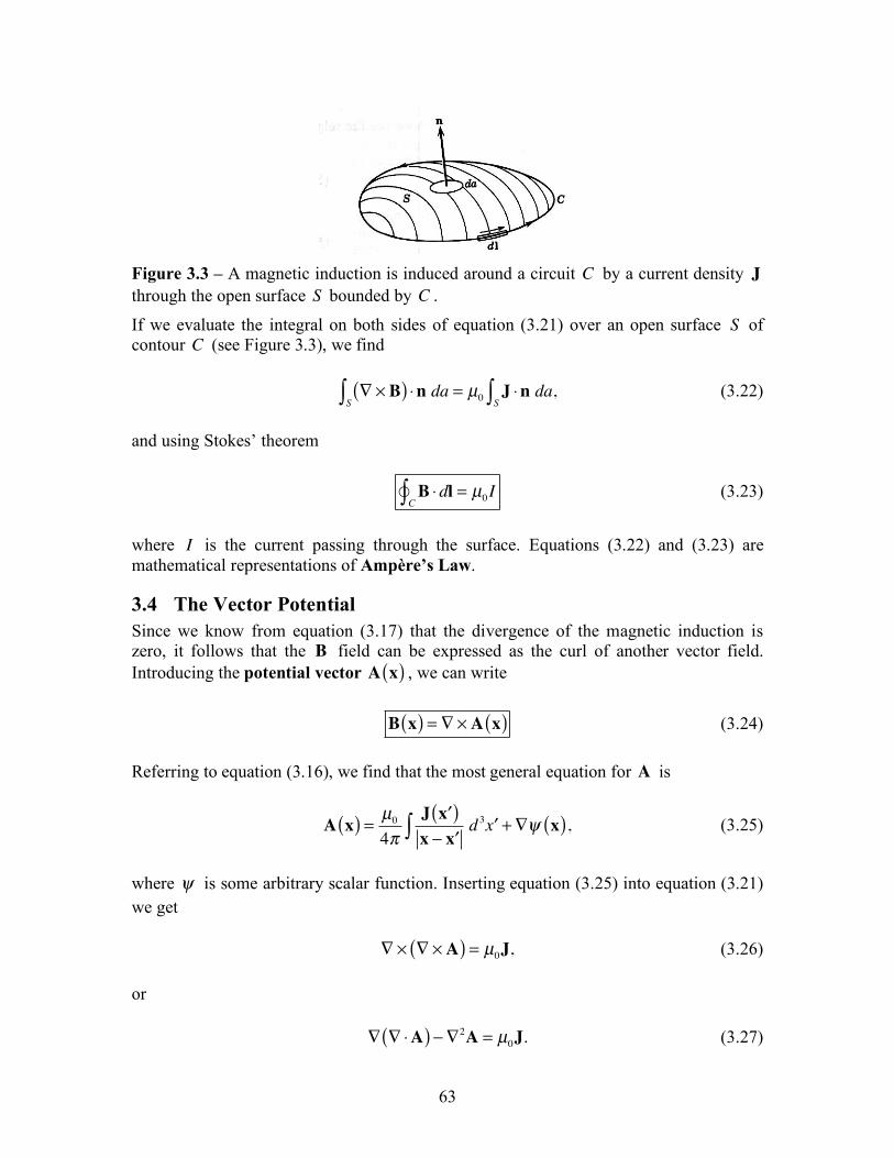
Figure 3.3 – A magnetic induction is induced around a circuit C by a current density J through the open surface S bounded by C .

If we evaluate the integral on both sides of equation (3.21) over an open surface S of contour C (see Figure 3.3), we find ! " B( ) #n da

S$ = µ

0J #n da

S$ , (3.22)

and using Stokes’ theorem

B !dlC!" = µ

0I (3.23)

where I is the current passing through the surface. Equations (3.22) and (3.23) are mathematical representations of Ampère’s Law.

3.4 The Vector Potential Since we know from equation (3.17) that the divergence of the magnetic induction is zero, it follows that the B field can be expressed as the curl of another vector field. Introducing the potential vector A x( ) , we can write B x( ) = ! " A x( ) (3.24) Referring to equation (3.16), we find that the most general equation for A is

A x( ) =µ0

4!J "x( )x # "x$ d

3 "x +%& x( ), (3.25)

where ! is some arbitrary scalar function. Inserting equation (3.25) into equation (3.21) we get ! " ! " A( ) = µ

0J, (3.26)

or ! ! "A( ) # !2

A = µ0J. (3.27)

64

But because of the freedom brought by the presence of !" in the equation defining the potential vector (i.e., equation (3.25)), we can choose ! "A to suit our needs. Using the so-called Coulomb gauge, which sets ! "A = 0 , we write !

2A = "µ

0J. (3.28)

Just as

! x( ) =1

4"#0

$ %x( )

x & %xd3 %x' , (3.29)

is the solution to the Poisson equation (i.e., !2" = #$ %

0), the following is the solution

to equation (3.28)

A x( ) =µ0

4!

J "x( )x # "x

d3 "x$ (3.30)

Equation (3.30) is valid in general, as we can set ! = cste due to the fact that ! "A = 0 reduces to !2" = 0 from equation (3.25). This is because

! "J #x( )

x $ #x% d3 #x = ! "

J #x( )

x $ #x

&

'()

*+% d3 #x

= $ #! "J #x( )

x $ #x

&

'()

*+% d3 #x ,

(3.31)

since !" # J !x( ) = 0 . Equation (3.31) vanishes from equation (3.20).

3.5 The Magnetic Dipole Moment Staying with the Coulomb gauge, and the resulting expression for the vector potential (i.e., equation (3.30)), we want to determine the multipole term (just as we did for the electrostatic potential) that will dictate the intensity of the vector potential at distances large compared to that of the current source. Therefore, assuming that x! !x in equation (3.30), we can use a Taylor series for the 1 x ! "x term around x . Using equation (1.85) we write

1

x ! "x=1

x+x # "x

x3+! (3.32)

65

Upon inserting this result in equation (3.30), the components of the vector potential can be approximated to

Aix( ) =

µ0

4!

1

xJi

"x( ) d 3 "x# +x

x3$ "x J

i"x( ) d 3 "x# +!

%

&''

(

)**. (3.33)

In order to transform this equation, consider the following expression

gJ ! "# f d3 "x$ = gJi "%i f d

3 "x$= "%i Ji fg( ) & fJi "%ig & fg "%i Ji'( )* d

3 "x$= "# ! Jfg( ) & fJ ! "# g & fg "# ! J'( )* d

3 "x$= fgJ !n d "a$ & fJ ! "# g + fg "# ! J[ ]$ d

3 "x ,

(3.34)

and if f and g are good functions, then the surface integral vanishes and we get gJ ! "# f + fJ ! "# g + fg "# ! J[ ]$ d

3 "x = 0. (3.35) We first set f = 1 and g = !xi into equation (3.35) to find that J !x( ) d 3 !x" = 0, (3.36) since !" # J !x( ) = 0 . Second, if f = !xi and g = !x j , then equation (3.35) yields !xiJ j + !x jJi( ) d 3 !x" = 0. (3.37) Inserting this last equation in the second integral on the right-hand side of equation (3.33) we have

x j !x jJi d3 !x" = #

1

2x j !xiJ j # !x jJi( ) d 3 !x"

= #1

2x j $ im$ jn # $ in$ jm( ) !xmJn d

3 !x"

= #1

2x j%kij%kmn !xmJn d

3 !x"

= #1

2x & !x & J( ) d 3 !x"'(

)*i.

(3.38)

The magnetization or magnetic moment density is defined as

66

M x( ) =1

2x ! J x( )"# $% (3.39)

and its volume integral, the magnetic moment with

m =1

2!x " J !x( ) d 3 !x# (3.40)

We note that if the current loop is located on a plane, then equation (3.40) transforms to

m =I

2!x " d !l!# , (3.41)

where I d !l is the current multiplied by the length element at !x . Since the quantity !x " d !l 2 represent the elemental area (a small triangle) subtended by the element d !l

at !x , then the magnitude of the magnetic dipole moment is m = I ! Area( ). (3.42) With the definitions given in equations (3.39) and (3.40), and equations (3.36) and (3.38), the vector potential expansion of equation (3.33) becomes

A x( ) =µ0

4!

m " x

x3

(3.43)

This is the lowest non-vanishing term in the expansion, and will therefore be dominant at large distances (i.e., x! !x ). Note that since there are no magnetic monopoles (see equations (3.33) and (3.36)), the value of the magnetic dipole moment is independent of the origin of the coordinate system since, from equation (3.36),

a + !x( ) " J !x( ) d 3 !x# = a " J !x( ) d 3 !x# + !x " J !x( ) d 3 !x#

= !x " J !x( ) d 3 !x# .

(3.44)

We are now in a position to evaluate the magnetic induction due to the dipole moment term using equation (3.24)

67

B = ! " A

=µ0

4#! "

m " xx3

$

%&

'

()

=µ0

4#!

1

x3

$

%&

'

() " m " x( ) +

1

x3! " m " x( )

*

+,,

-

.//

=µ0

4#03x " m " x( )

x5

+1

x3! " m " x( )

*

+,,

-

.//.

(3.45)

But since

x ! m ! x( )

x5

=x2m " x m #x( )

x5

, (3.46)

and

! " m " x( ) = m ! #x( ) $ x ! #m( ) + x #!( )m $ m #!( )x

= 3m $m = 2m, (3.47)

since m does not depend on the coordinates, then equation (3.45) becomes

B x( ) =µ0

4!

3n n "m( ) #m

x3

$

%&&

'

()), (3.48)

where n = x x . Just as we did for the derivation of the electric field due to an electric dipole in section 2.3, we consider the volume integral of the magnetic induction. If the volume (defined as a sphere of surface S and radius R ) encloses the dipole moment, it can be seen, for the same reasons enumerated in the discussion leading to equation (2.97), that B x( ) d 3x

r<R! = 0 (3.49)

when equation (3.48) is used. We can, however, also calculate

B x( ) d 3x

r<R! = " # A x( ) d 3xr<R!

= R2n # A x( ) d$

S! ,

(3.50)

where equation (1.31) was used, and n , this time, is the unit vector normal to the surface S . Inserting equation (3.30) into equation (3.50) we get

68

B x( ) d 3xr<R! = "

µ0

4#R2d3 $x J $x( ) %

n

x " $xd&

S!! . (3.51)

Using the results obtained from equations (2.101) to (2.106), we can write

B x( ) d 3xr<R! =

µ0

3R2

r<

r>2

"n # J "x( ) d 3 "x!

=µ0

3

R2r<

"r r>2

$

%&'

()"x # J "x( ) d 3 "x! .

(3.52)

Since we assumed that the current distribution is entirely contained in the sphere, then r<= !r and r

>= R and equation (3.52) reduces to

B x( ) d 3xr<R! =

2µ0

3m. (3.53)

We combine this result with that from equation (3.48) to write our final equation for the magnetic induction due to a magnetic dipole moment

B x( ) =µ0

4!

3n n "m( ) #m

x3

+8!

3m$ x( )

%

&''

(

)**

(3.54)

Going back to equation (3.52), when the current distribution is entirely located outside the sphere (i.e., r

>= !r and r

<= R ), we find from equation (3.13) that

B x( ) d 3xr>R! =

4"R3

3B 0( ). (3.55)

3.6 The Force and Torque on, and the Potential Energy of, a Magnetic Dipole Moment in an External Magnetic Induction

We now consider a current distribution that is subjected to an external magnetic induction B . From equations (3.12) we see that the force and the torque experienced by a current distribution are proportional to the intensity of the magnetic induction. If the size of the volume occupied by the current distribution is significantly smaller than the scale over which B varies, it is to our advantage to use a Taylor expansion to approximate the components of the magnetic induction around a suitable origin

Bkx( ) = B

k0( ) + x !"B

k x=0+! (3.56)

Then, from the first of equations (3.12), we can express the components of the force felt by the current distribution as

69

Fi = !ijk Bk 0( ) J j "x( ) d 3 "x# + J j "x( ) "x $ "% Bk "x =0d3 "x +!#&

'()

= !ijk %Bk 0( ) $ "x J j "x( ) d 3 "x +!#&'

(),

(3.57)

from equation (3.36), and where !B

k0( ) " #! B

k #x =0. Using equations (3.38) (replacing x

with !Bk0( ) ) and (3.40), we find that the dominant term for the force is

F = m ! "( ) ! B x( ), (3.58) where it is understood that after differentiation of the magnetic induction, x must be set to zero. Equation (3.58) can be further simplified with F = m ! "( ) ! B x( ) = " m #B( ) $m " #B( ), (3.59) but since ! "B = 0 , we find that F = ! m "B( ) (3.60) Defining the force as the negative of the gradient of the potential energy U , we can express the latter as U = !m "B (3.61) It is important to realize that equation (3.61) does not represent the total energy of a magnetic dipole moment in an external B field, since work must be done to keep m constant (through the current that produces the dipole) when bringing the dipole to its final position in the field. When using equations (3.12) and (3.56) to evaluate the torque N on the dipole due to the external magnetic induction, we find that the lowest order term does not vanish and, therefore, dominates. More precisely, we find that

N = !x " J !x( ) " B 0( )#$ %& d

3 !x'= !x (B 0( )#$ %&J !x( ) ) !x ( J !x( )#$ %&B 0( ){ } d 3 !x' .

(3.62)

The first integral on the right-hand side of the second of equations (3.62) is readily transformed using equation (3.38) (replacing x with B 0( ) ). To solve the second integral we revert once again to equation (3.35) while setting f = g = !r . Then,

70

fJ ! "# g d3 "x$ = "r J ! "# "r d

3 "r$

= "r J !"x

"rd3 "r$

= J ! "x d3 "r$ ,

(3.63)

and we find upon inserting this result in equation (3.35) that 2 J ! "x d

3 "r# = $ "r 2 "% ! J d 3 "x# = 0, (3.64) since !" # J = 0 . The expression for the torque reduces to N = m ! B 0( ) (3.65) It is interesting to note that if the magnetic dipole moment makes an angle ! with the magnetic induction, then from equation (3.61) we have that U = !mBcos "( ). (3.66) If we now calculate the negative of the derivative of the potential energy with respect to ! we get

!dU

d"= !mBsin "( )

= m # B 0( )

= N .

(3.67)

We find that the dipole tends to settle (i.e., when dU d! = 0 and N = 0 ) itself parallel to the field (i.e., when sin !( ) = 0 ). From equation (3.66) we see that this is the lowest energy configuration.

3.7 The Macroscopic Equations, the Magnetic Field H , and the Boundary Conditions

Just as we introduced macroscopic equations and the electric displacement D when studying electrostatics, we do the same here with the introduction of the magnetic field H and the corresponding macroscopic equations of magnetostatics. So, we again define a new set of fields and average quantities. For example, if we have a microscopic magnetic induction Bµ that we average over a volume element !V , then the resulting macroscopic field is

71

B =1

!VBµ x + "x( ) d 3 "x

!V# . (3.68)

Taking the divergence on both sides of this equation reveals that the macroscopic magnetic induction is, like the its microscopic counterpart, divergence-less (see equations (2.128) and (2.129)). That is, ! "B = 0, (3.69) and we can define a macroscopic vector potential A such that B = ! " A. (3.70) If we now consider a medium made up of a large number of molecules or atoms of type i , and each with its own magnetic moment m

i, we can then define the average

macroscopic magnetization or magnetic moment density as M x( ) = N

im

i

i

! , (3.71)

where N

i is the average number per unit volume of particles of type i , and m

i is the

average magnetic moment at location x . The vector potential resulting from the bulk magnetization expressed through equation (3.71) (multiplied by the element of volume !V containing the medium) can be calculated with equation (3.43). In general, however, there will not only exist a magnetization, but also a current density J x( ) that can give rise to a vector potential, as shown in equation (3.30). Therefore, the total vector potential from a small volume !V is given by

!A x( ) =µ0

4"

J #x( )!Vx $ #x

+M #x( )!V % x $ #x( )

x $ #x3

&

'((

)

*++. (3.72)

Taking the limit when !V " 0 and integrating, then equation (3.72) is transformed to

A x( ) =µ0

4!J "x( )x # "x

+M "x( ) $ x # "x( )

x # "x 3

%

&''

(

)**d3 "x+

=µ0

4!J "x( )x # "x

+M "x( ) $ ",1

x # "x

-

./0

12%

&''

(

)**d3 "x+ ,

(3.73)

and upon using the general relation ! " #a( ) = !# " a +#! " a and equation (1.31) to modify the second integral on the right-hand side we have

72

A x( ) =µ0

4!J "x( )x # "x

# "$ %M "x( )x # "x

&

'()

*++

"$ %M "x( )x # "x

,

-..

/

011d3 "x2

=µ0

4!J "x( ) + "$ %M "x( )

x # "x,

-.

/

01 d

3 "x2 #µ0

4!"n %

M "x( )x # "x

&

'()

*+d "a

S2 ,

(3.74)

and since, as usual, the surface integral vanishes we finally get

A x( ) =µ0

4!

J "x( ) + "# $M "x( )x % "x

&

'(

)

*+ d

3 "x, (3.75)

This equation is similar in form to the microscopic counterpart previously evaluated that links the current density and the vector potential (see equation (3.30)), and we can therefore write down the differential equation equivalent to this integral as ! " B = µ

0J +! "M[ ]. (3.76)

It is seen from equation (3.76) that the magnetization contributes an effective current density J

M defined as

J

M= ! "M, (3.77)

and that a total macroscopic current density J + J

M could also be introduced.

Alternatively, the curl of the magnetization can be combined with the magnetic induction to form a new quantity H called the magnetic field

H =1

µ0

B !M (3.78)

Using this definition for the magnetic field, the macroscopic equations for magnetostatics can be written as

! "H = J

! #B = 0 (3.79)

For isotropic paramagnetic and diamagnetic media (more on these in the second assignment) there is a simple linear relation between the magnetic induction and the magnetic field B = µH (3.80)

73

where µ is the permeability of the medium under consideration. The ratio µ µ0

(> 1 for paramagnetic substances and < 1 for diamagnetic substances) typically differs from unity by only a few parts in 105 . This simple picture is, however, not valid for every substances. For example, ferromagnetic media have a permeability such that

µ µ

0! 1,

with a non-linear relationship between B and H . The phenomenon known as hysteresis (i.e., the lack of a one-to-one correspondence between B and H ) is commonly observed in their response.

The boundary conditions for the components of the magnetic induction and the magnetic field can be derived using Figure 1.3, and the divergence and Stokes’ theorems. The continuity of the normal components of the magnetic induction at the boundary between two media (labeled 1 and 2) can be verified using the small pillbox of Figure 1.3, which straddles the interface between regions 1 and 2. The volume integral of the last of equations (3.79) reduces to (using the divergence theorem) ! "B d 3x

V# = B "da

S# = 0, (3.81)

where n is a unit vector normal to the boundary that extends from region 1 to region 2. In the limit where the height of the box goes to zero, the surface integral of the magnetic induction reduces to B

2! B

1( ) "n = 0, (3.82) which verifies the aforementioned continuity of the normal components of the magnetic induction at the boundary between two media. If we now consider the integral of the first of equations (3.79) over an open surface of contour C that also straddles the boundary between the two media, as shown in Figure 1.3, we find (using Stokes’ theorem) that

! "H( ) # t da

S$ = H #dl

C!$ = J # t da

S$ , (3.83)

where t is a unit vector normal to the open surface and parallel to the boundary. In the limit where the two segments of C that are parallel to n become infinitesimally short, we get

H !dl

C!" = t # n( ) ! H2

$H1( ) %l, (3.84)

and J ! t da

S" = K ! t #l, (3.85)

where !l is the length of the segments of C that are parallel to the boundary, and K is the idealized surface current density, which exist at the interface between the two regions. Since a ! b " c( ) = b ! c " a( ) , equations (3.83), (3.84), and (3.85) can be shown to yield

74

n ! H

2"H

1( ) = K. (3.86) That is, the tangential components of the magnetic field are discontinuous at the boundary, and are related to each other through the surface current density in the manner shown in equation (3.86).

3.8 Faraday’s Law of Induction We now leave the domain of strictly static phenomena to consider systems where there can be a time-dependency for some quantities. In particular we study the results obtained by Faraday and contained in the law famously named after him. If we consider a circuit C bounded by an open surface S threaded by a magnetic induction B , as shown in Figure 3.4, we know from Faraday’s experiment that if the flux of B changes with time, then an electric field is induced along the circuit according to Faraday’s law of induction

E = !E "dlC!# = $k

d

dtB "n da

S# , (3.87)

where E is the electromotive force that causes a current to flow around the circuit, !E is the induced electric field at the element dl , and k is a constant. The surface integral on the right-hand side of equation (3.87) is the magnetic flux. This law of induction can apply to many experimental situations. For example, it could be that:

1) The circuit C is unchanging but the magnetic induction is time varying (i.e., !B !t " 0 ).

2) The circuit C is unchanging but dragged across an inhomogeneous magnetic induction (i.e., !B !t = 0 ).

3) The circuit is deformed in time and the magnetic induction can be homogeneous and time-independent.

In considering the different choices enumerated above, it should become clear that one must be careful when calculating the (total) time derivative present in Faraday’s law.

Figure 3.4 – Magnetic flux linking a circuit C .

75

More precisely, let us concentrate on a quantity Q x,t( ) , which can vary with time and position. An observer moving at a velocity v would measure the changes in Q as function of time along its path to be

dQ

dt= lim

!t"0

1

!tQ x,t + !t( ) #Q x,t( ) +Q x + v!t,t( ) #Q x,t( )$% &'. (3.88)

Using Taylor expansions to approximate the terms contained in the brackets we get

dQ

dt= lim

!t"0

1

!t

#Q x,t( )

#t!t +

#Q x,t( )

#xivi!t

$

%&

'

(), (3.89)

or more compactly

dQ x,t( )

dt=!Q x,t( )

!t+ v "#( )Q x,t( ). (3.90)

In general, the total time derivative is defined by

d

dt!

"

"t+ v #$, (3.91)

and it is often called the Lagrangian derivative. This is the form of the time derivative that must be used in equation (3.87) since it takes into account variations due to both implicit time dependencies (i.e., ! !t ) and motions (i.e., v !" ). Applying the Lagrangian derivative to the magnetic induction we get

dBi

dt=!Bi!t

+!x j!t

!Bi!x j

=!Bi!t

+!!x j

Bi!x j!t

"#$

%&'( Bi

!2x j!x j!t

=!Bi!t

+!!x j

Bivj( ),

(3.92)

since

!2x j!xk!t

=!!t

!x j!xk

"

#$%

&'=

!!t

( jk( ) = 0. (3.93)

76

Furthermore, if we combine to this last equation the fact that !Bj!x

j= 0 , we can also

write that ! Bjvi( ) !x

j= 0 and subtract this term to the right-hand side of equation (3.92)

without changing its content. Therefore,

dBi

dt=!Bi

!t+

!

!x jBivj( ) "

!

!x jBjvi( )

=!Bi

!t+ # im# jn " # in# jm( )

!

!x jBmvn( )

=!Bi

!t+ $kij$kmn

!

!x jBmvn( ),

(3.94)

or alternatively

dB

dt=!B

!t+" # B # v( ). (3.95)

Using this result to evaluate the surface integral of equation (3.87), we find

d

dtB !n da

S" =

#B

#t+$ % B % v( )

&

'()

*+!n da

S"

=#B

#t!n da

S" + B % v( )

C!" !dl,

(3.96)

where Stokes’ theorem was used for the last step, and the velocity v is defined as that of the circuit. Inserting equation (3.96) into equation (3.87), we can transform Faraday’s law to

!E " k v # B( )$% &'C!( )dl = "k

*B

*t)n da

S( . (3.97)

It is seen that the left-hand side of equation (3.97) contains the contribution due to the motion of the circuit. However, for a stationary observer not moving with the circuit, the only term that can be responsible for the induction of an electric field E will be that due to the possible time dependency of the magnetic induction. This is exactly the term present on the right-hand side of equation (3.97). Therefore, we can also write

EC!! "dl = #k

$B

$t"n da

S! . (3.98)

Equating the left-hand sides of the last two equations we get !E = E + k v " B( ). (3.99)

77

To evaluate the constant k we go back to more restrictive conditions where the magnetic induction is homogeneous and time independent (i.e., !B !t = 0 ), but we still consider a circuit moving with a velocity v relative to a stationary observer. From equation (3.97), we see that force !F experienced by a charge q at rest in the moving circuit is given by !F = q !E = kq v " B( ). (3.100) On the other hand, since the charge is moving at velocity v relative to the frame of reference of the stationary observer, it is seen by this observer to be equivalent to a current density J = qv! x " x

0( ) (x0 is the instantaneous position of the charge). Then,

using the first of equations (3.12) for the force F measured by this observer, we find that

F = qv! x " x

0( ) # B x( ) d 3x0$

= qv # B x0( ).

(3.101)

However, because the position of the charge in two frames of reference is related through a coordinate transformation that is a linear function of time (i.e., x

0= !x

0+ vt ) and that

the force is proportional to the second derivative of the position, therefore it must be that F = !F . (3.102) Equating equations (3.100) and (3.101), we find that k = 1 (in SI units). Faraday’s law of induction then becomes

!E "dlC!# = $

d

dtB "n da

S# (3.103)

and we also obtain, as a result of this analysis, an expression for the force F acting on a charge q moving at a velocity v , and subjected to an electric field E and a magnetic induction B . That is, we have the so-called Lorentz force F = q E + v ! B( )"# $% (3.104)

We can put Faraday’s law in a differential form using equation (3.98) (with k = 1 ), since E and B must be evaluated in the same frame of reference, and Stokes’ theorem. Then,

! " E +#B#t

$%&

'()*n da

S+ = 0, (3.105)

but since the circuit C and the unit normal vector n are arbitrary, we can write

78

! " E +#B

#t= 0 (3.106)

3.9 Energy in the Magnetic Field Now that we have analyzed the effect of a changing magnetic flux on a circuit through Faraday’s law of induction, we are in a position to investigate the question of the energy contained in the magnetic field. We want to calculate the work needed to bring the currents and fields from an initial value of zero to their steady state values. In doing so, electromotive forces will be induced that will require the sources of current to do work to establish the steady state. So, it is best to start by simply considering a single circuit and its reaction to a change in magnetic flux. We already know that if the magnetic flux linking a circuit changes, then an electromotive force will be induced around the circuit. The flux F linking the circuit is given by F = B !n da

S" , (3.107)

and using equation (3.87) we can write (with k = 1 )

E = !E "dlC!# = $

dF

dt, (3.108)

where the negative sign is used to specify that the induced field (and current) opposes the flux change through the circuit (the so-called Lenz’ law). Since the time rate of change in the energy (or the power) of a charged particle moving at velocity v and subjected to a force F is

dE

dt= F !v, (3.109)

and that the electric field !E induced by the magnetic flux change is related to the force through F = q !E , then the time rate of change in the energy of the particle can be expressed as

dE

dt= qv ! "E . (3.110)

To keep the charge moving at the same velocity, the sources of the circuit will have to do an amount of work equal to the energy change of equation (3.110), but of opposite sign (so that the total time rate in energy change is zero). If we now sum on all the charges around the circuit, we can evaluate the rate at which work must be done by the sources using the following equation (with qv = qdl dt! I dl )

79

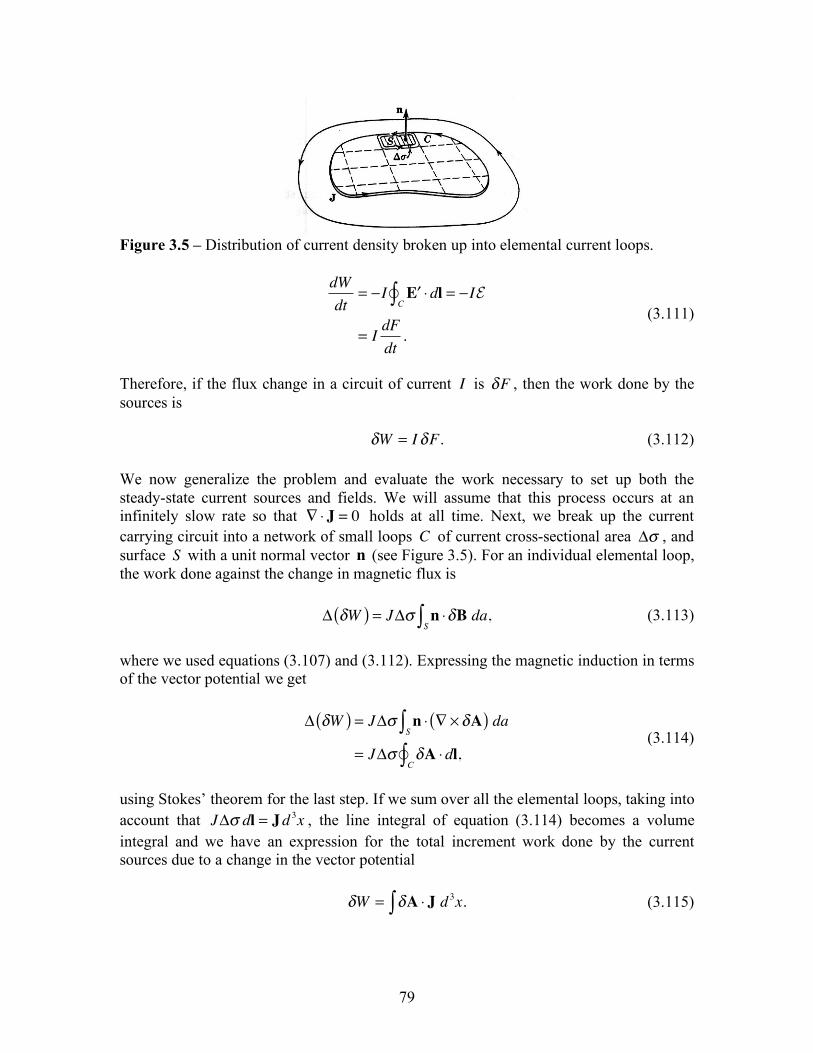
Figure 3.5 – Distribution of current density broken up into elemental current loops.

dW

dt= !I "E #dl

C!$ = !IE

= IdF

dt.

(3.111)

Therefore, if the flux change in a circuit of current I is !F , then the work done by the sources is !W = I!F. (3.112) We now generalize the problem and evaluate the work necessary to set up both the steady-state current sources and fields. We will assume that this process occurs at an infinitely slow rate so that ! " J = 0 holds at all time. Next, we break up the current carrying circuit into a network of small loops C of current cross-sectional area !" , and surface S with a unit normal vector n (see Figure 3.5). For an individual elemental loop, the work done against the change in magnetic flux is ! "W( ) = J!# n $"B da

S% , (3.113)

where we used equations (3.107) and (3.112). Expressing the magnetic induction in terms of the vector potential we get

! "W( ) = J!# n $ % & "A( ) daS'

= J!# "A $dlC!' ,

(3.114)

using Stokes’ theorem for the last step. If we sum over all the elemental loops, taking into account that J!" dl = Jd 3x , the line integral of equation (3.114) becomes a volume integral and we have an expression for the total increment work done by the current sources due to a change in the vector potential !W = !A " J d 3x.# (3.115)

80

We can substitute the magnetic field for the current density using the first of equations (3.79), and we get

!W = !A " # $H( ) d 3x%

= # " H $ !A( ) +H " # $ !A( )&' () d3x% ,

(3.116)

since ! " a # b( ) = b " ! # a( ) $ a " ! # b( ) . The first integral on the right-hand side of equation (3.116) can be transformed into a surface integral through the divergence theorem and will, therefore, vanish if the field distribution is localized; we are then left with

!W = H " # $ !A( ) d 3x%= H "!B d 3x%

=1

2! H "B( ) d 3x% .

(3.117)

The last of equations (3.117) was made possible with the assumption that the relation B = µH holds (i.e., the medium is para- or diamagnetic). Integrating equation (3.117) from the initial (zero) to the final values of the fields, we find that the total magnetic energy is

W =1

2H !B d 3x" (3.118)

Alternatively, we can express the energy with J and A starting with equation (3.115), and proceeding in the same manner as was done in equations (3.117) and (3.118) as long as J and A are linearly related. Then,

W =1

2J !A d

3x" . (3.119)

Finally, we consider the change in energy when an object of permeability µ

1 is inserted

in a region of permeability µ0 where a fixed magnetic induction B

0 already exists. We

assume that there are no current density distributions J . That is, ! "H = ! "H

0= 0. (3.120)

If the object were absent, the energy contained within the equivalent volume of space V

1

it occupies would be

81

W0=1

2H0!B

0d3x

V1" , (3.121)

whereas it would become

W1=1

2H !B d 3x

V1" (3.122)

with it in place. The difference between the two energies (which represents the energy stored in the object) is

W !W

1"W

0=1

2H #B "H

0#B

0( ) d 3xV1$

=1

2B #H

0" B

0#H( ) d 3x

V1$ +

1

2B + B

0( ) # H "H0( ) d 3x

V1$ .

(3.123)

However, since we can write B + B

0= ! " A , and ! " H #H

0( ) = 0 , the second integral on the right-hand side of equation (3.123) is shown to vanish with

B + B0( ) ! H "H

0( ) d 3xV1# = $ % A( ) ! H "H

0( ) d 3xV1#

= $ ! A % H "H0( )&' () + A !$ % H "H

0( ){ } d 3xV1#

= A % H "H0( )&' () !n da

S1#

= 0,

(3.124)

where the integral of the divergence term was transformed into a surface integral over S

1,

the surface delimiting the volume V1, which vanishes because H = H

0 at the surface (or

just beyond it). Hence,

W =1

2B !H

0"H !B

0( ) d 3xV1# . (3.125)

If the region occupied by the object belongs to free space (i.e., the permeability µ

0 is that

of vacuum), then

W =1

2

1

µ0

B !H"

#$%

&'(B

0d3x

V1) , (3.126)

and from equation (3.78)

82

W =1

2M !B

0d3x

V1" (3.127)

The difference between equation (3.127) and equation (3.61) for a permanent magnetic dipole moment in an external magnetic induction comes from the fact equation (3.127) takes into account the work needed to create the magnetic moment and keeping it constant, while equation (3.61) is only concerned with establishing the permanent dipole in the external field.