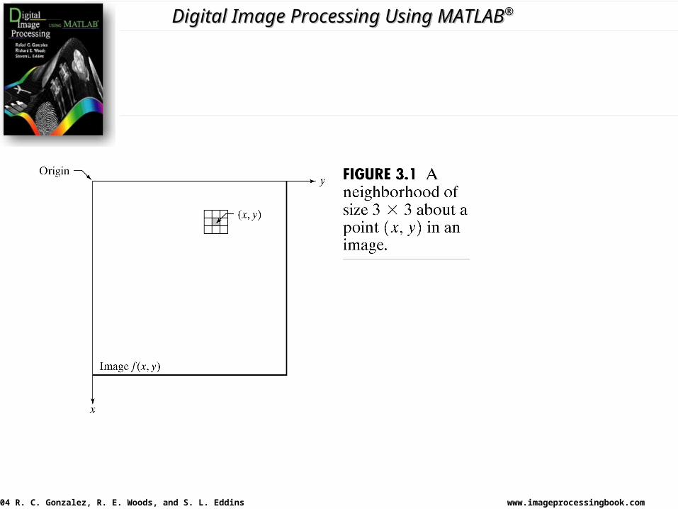
www.imageprocessingbook.com 04 R. C. Gonzalez, R. E. Woods, and S. L. Eddins Digital Image Processing Using MATLAB ® Chapter 3 Intensity Transformations and Spatial Filtering • O capítulo trata-se de transformações no domínio espacial: transformações de intensidade e filtragem espacial.

Chapter 3 Intensity Transformations and Spatial Filtering
Mar 18, 2016
O capítulo trata-se de transformações no domínio espacial: transformações de intensidade e filtragem espacial. Chapter 3 Intensity Transformations and Spatial Filtering. Função imadjust - PowerPoint PPT Presentation
Welcome message from author
This document is posted to help you gain knowledge. Please leave a comment to let me know what you think about it! Share it to your friends and learn new things together.
Transcript

www.imageprocessingbook.com© 2004 R. C. Gonzalez, R. E. Woods, and S. L. Eddins
Digital Image Processing Using MATLAB®
Chapter 3Intensity Transformations
and Spatial Filtering
• O capítulo trata-se de transformações no domínio espacial:
transformações de intensidade e filtragem espacial.
www.imageprocessingbook.com© 2004 R. C. Gonzalez, R. E. Woods, and S. L. Eddins
Digital Image Processing Using MATLAB®

www.imageprocessingbook.com© 2004 R. C. Gonzalez, R. E. Woods, and S. L. Eddins
Digital Image Processing Using MATLAB®
• Função imadjust
A função imadjust é uma ferramenta básica em IPT para transformações de imagens em escala de cinza.
Sintaxe: g = imadjust (f, [low_in high_in], [low_out high_out], gamma)
• Como mostrado na Fig. 3.2 essa função mapeia os valores de intensidade da imagem f para novos valores em g, tal que os valores entre low_in e high_in mapeiem entre low_out e high_out.
• Valores abaixo de low_in e acima de high_in são cortados; isto é, valores abaixo de low_in mapeiam em low_out, e valores acima de high_in mapeiam em high_out.
• A imagem de entrada pode ser da classe uint8, uint16, ou double, e a imagem de saída tem a mesma classe da imagem de entrada.
www.imageprocessingbook.com© 2004 R. C. Gonzalez, R. E. Woods, and S. L. Eddins
Digital Image Processing Using MATLAB®
Chapter 3Intensity Transformations
and Spatial Filtering
www.imageprocessingbook.com© 2004 R. C. Gonzalez, R. E. Woods, and S. L. Eddins
Digital Image Processing Using MATLAB®
• Todos os valores dos parâmetros, exceto f, são especificados como valores entre 0 e 1, independente da classe de f.
• Se f é da classe uint8, imadjust multiplica os valores por 255 para determinar o valor a ser usado;
• Se f é da classe uint16 os valores são multiplicados por 65535.• Usando a matriz vazia [ ] para [ low_in high_in] ou para [ low_out high_out]
resulta nos valores default [0 1].• Se high_out é menor que low_out, a intensidade de saída é invertida.• O parâmetro gamma especifica a forma da curva que mapeia os valores de
intensidade. Se gamma é menor que 1, o mapeamento clareia os valores de saída; se gamma é maior que 1, o mapeamento escurece os valores de saída; e se o argumento gamma é omitido, o valor default é 1, mapemento linear.

www.imageprocessingbook.com© 2004 R. C. Gonzalez, R. E. Woods, and S. L. Eddins
Digital Image Processing Using MATLAB®
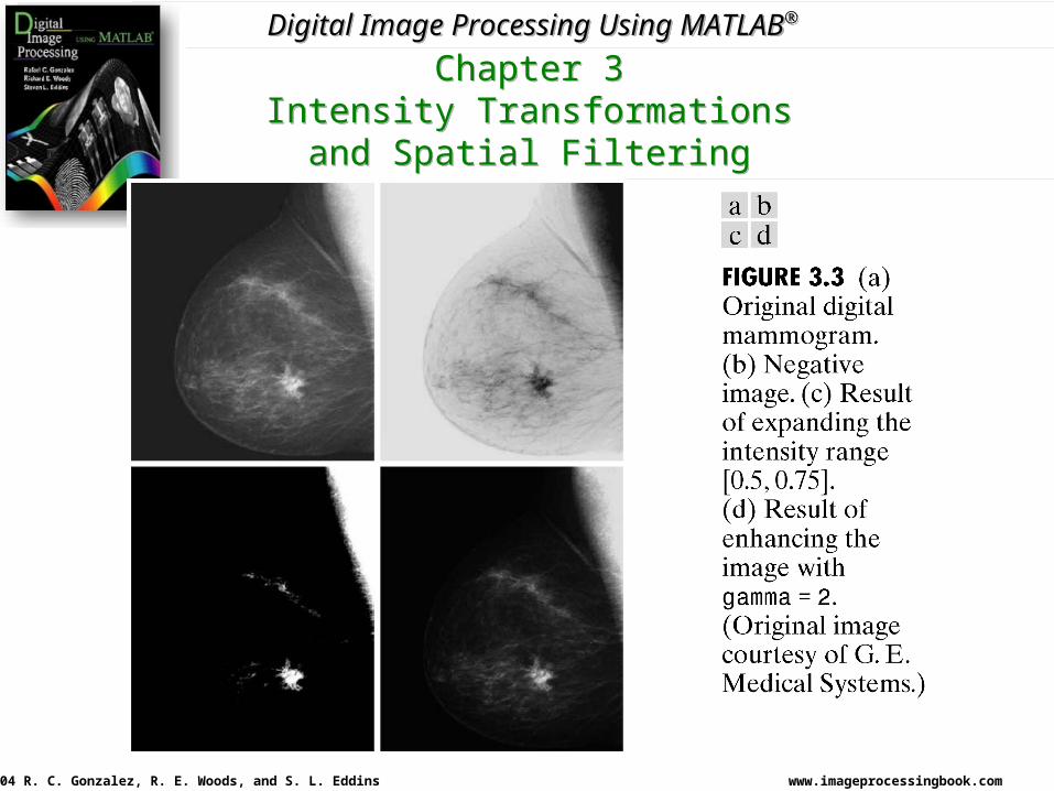
• Fig. 3.3a é uma imagem de mamograma, f.• A Fig. 3.3b mostra o negativo, obtido usando o comando: g1 = imadjust(f,[0 1],[1 0]); útil para detalhe branco ou cinza no meio de uma região predominantemente escura.• O negativo de uma imagem pode ser obtido também com a função: g = incomplement(f).• A Fig. 3.3c mostra o resultado usando o comando g2 = imadjust(f, [0.5 0.75],[0 1]), que aumenta o contraste para o intervalo de
interesse.• Finalmente o comando g3 = imadjust(f,[], [], 2); produz um resultado similar ao da Fig.3.3c, comprimindo o low end e expandindo
o high end da escala de cinza (Fig. 3.3d).
www.imageprocessingbook.com© 2004 R. C. Gonzalez, R. E. Woods, and S. L. Eddins
Digital Image Processing Using MATLAB®
Chapter 3Intensity Transformations
and Spatial Filtering
www.imageprocessingbook.com© 2004 R. C. Gonzalez, R. E. Woods, and S. L. Eddins
Digital Image Processing Using MATLAB®
• TRANSFORMAÇÕES LOGARITMICAS E DE EXTENSÃO DE CONTRASTE• A transformação logaritmica é implementada por
g = c* log(1 + double(f)), onde c = constante.
• Um dos principais usos dessa transformação é comprimir o intervalo dinâmico. • Por exemplo, o espectro de Fourier pode ter valores no intervalo [0, 106] ou maior.• Quando mostrado num monitor a imagem é mapeada linearmente para 8 bits, e os maiores
valores dominam a tela, resultando em detalhes perdidos para os valores baixos. Computando o logaritmo 106 é reduzido para aproximadamente 14, que é muito mais manipulável.
• Quando é feita uma transformação logaritmica, é desejável trazer o resultado de volta para o intervalo completo do display. Para 8 bits, a forma mais fácil é
gs = im2uint8(mat2gray(g));
www.imageprocessingbook.com© 2004 R. C. Gonzalez, R. E. Woods, and S. L. Eddins
Digital Image Processing Using MATLAB®
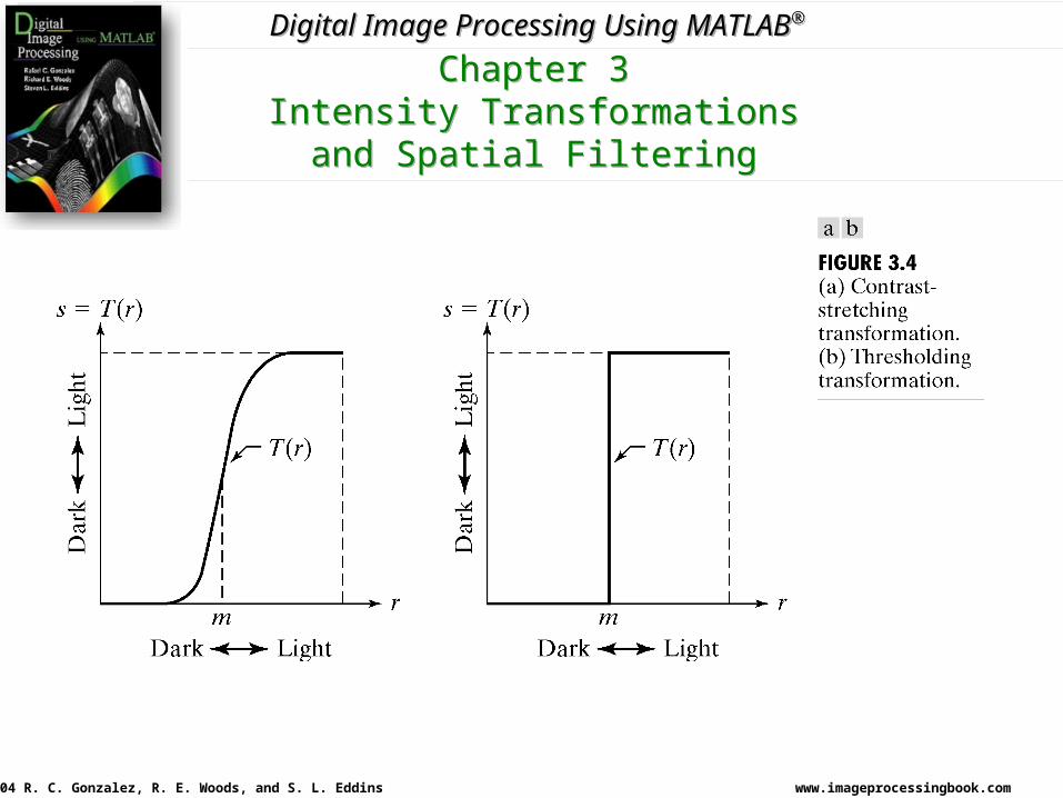
• A função da Fig. 3.4a é chamada de transformação de extensão de contraste (contrast stretching), porque o resultado é um alto contraste.
• No caso limite da Fig. 3.4b a saída é uma imagem binária.• A função da Fig. 3.4a tem a forma
onde r representa a intensidade da imagem de entrada e E controla a inclinação da função. Essa função é implementada usando o comando
g = 1./(1+(m./(double(f) + eps)).^E)
• Nota-se o uso do eps (ver Tabela 2.10) que corresponde à precisão relativa da representação ponto-flutuante, para prevenir o overflow se f for zero.
• Como valor limite de T(r) é 1, os valores de saída estão mapeados no intervalo [0,1]. A forma da Fig. 3.4a foi obtido com E = 20.
ErmrTs
)/(11)(
www.imageprocessingbook.com© 2004 R. C. Gonzalez, R. E. Woods, and S. L. Eddins
Digital Image Processing Using MATLAB®
Chapter 3Intensity Transformations
and Spatial Filtering
www.imageprocessingbook.com© 2004 R. C. Gonzalez, R. E. Woods, and S. L. Eddins
Digital Image Processing Using MATLAB®
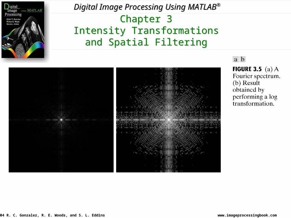
• EXEMPLO
• A Fig. 3.5a é um espectro de Fourier com valores no intervalo de 0 a 1.5x10⁶, mostrado num sistema de mapeamento linear de 8 bits.
• A Fig. 3.5b mostra o resultado obtido usando o comando
g= im2uint8(mat2gray(log(1+ double(f))));
www.imageprocessingbook.com© 2004 R. C. Gonzalez, R. E. Woods, and S. L. Eddins
Digital Image Processing Using MATLAB®
Chapter 3Intensity Transformations
and Spatial Filtering
www.imageprocessingbook.com© 2004 R. C. Gonzalez, R. E. Woods, and S. L. Eddins
Digital Image Processing Using MATLAB®
• ALGUMAS M-FUNCTIONS PARA TRANSFORMAÇÕES DE INTENSIDADE
• Manipulando um número variável de entradas e/ou saídas:• para verificar o número de argumentos que entram numa M-function usar
a função nargin n = nargin• Similarmente a função nargout é usada como número de saídas de uma M-
function. n = nargout• Por exemplo, supondo que a seguinte M-function foi executada: T = testhv(4,5);• O uso do nargin deve retornar 2, enquanto que o uso de nargout deve
retornar 1.
www.imageprocessingbook.com© 2004 R. C. Gonzalez, R. E. Woods, and S. L. Eddins
Digital Image Processing Using MATLAB®
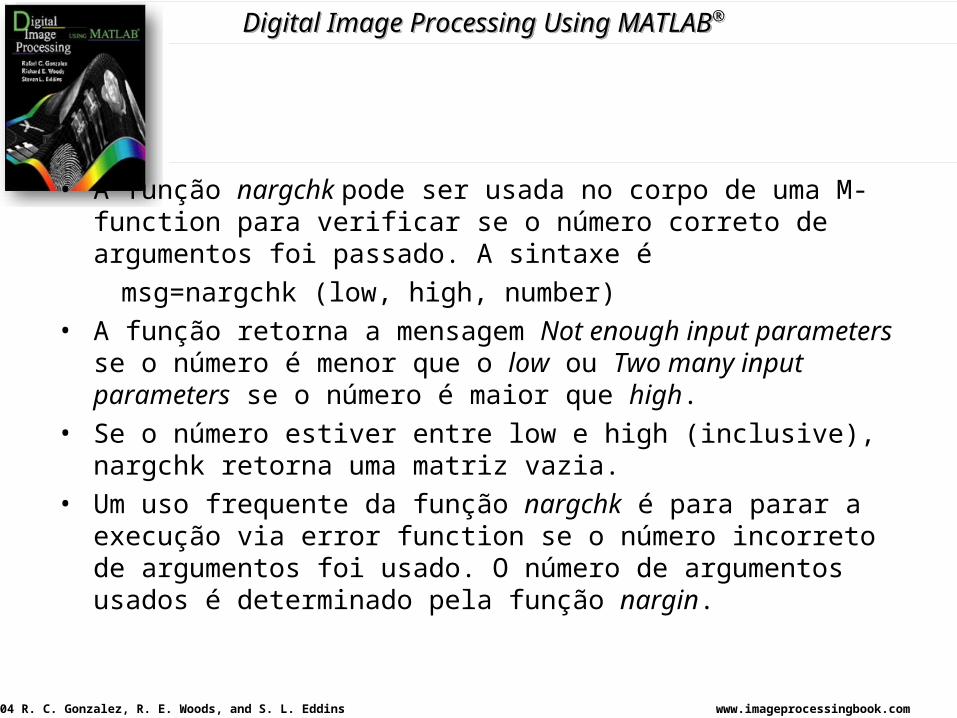
• A função nargchk pode ser usada no corpo de uma M-function para verificar se o número correto de argumentos foi passado. A sintaxe é
msg=nargchk (low, high, number)• A função retorna a mensagem Not enough input parameters se o número é
menor que o low ou Two many input parameters se o número é maior que high.
• Se o número estiver entre low e high (inclusive), nargchk retorna uma matriz vazia.
• Um uso frequente da função nargchk é para parar a execução via error function se o número incorreto de argumentos foi usado. O número de argumentos usados é determinado pela função nargin.
www.imageprocessingbook.com© 2004 R. C. Gonzalez, R. E. Woods, and S. L. Eddins
Digital Image Processing Using MATLAB®
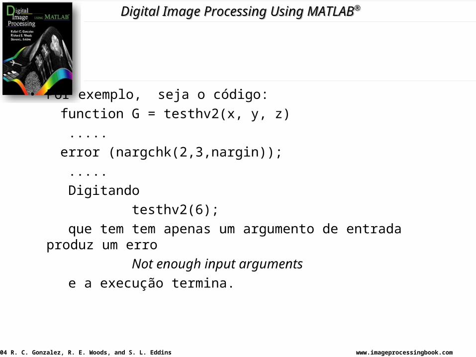
• Por exemplo, seja o código: function G = testhv2(x, y, z) ..... error (nargchk(2,3,nargin)); ..... Digitando testhv2(6); que tem tem apenas um argumento de entrada produz um erro Not enough input arguments e a execução termina.
www.imageprocessingbook.com© 2004 R. C. Gonzalez, R. E. Woods, and S. L. Eddins
Digital Image Processing Using MATLAB®
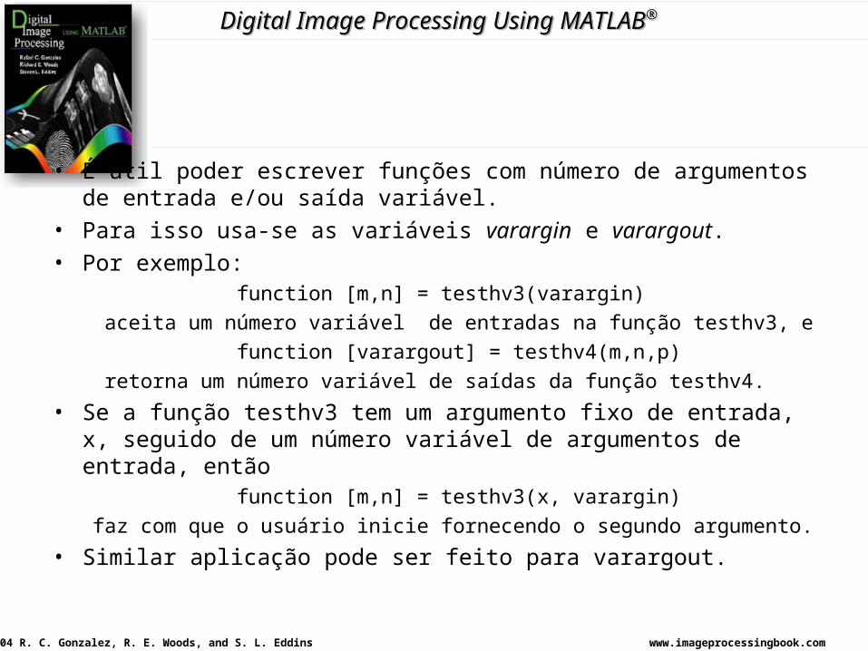
• É útil poder escrever funções com número de argumentos de entrada e/ou saída variável.
• Para isso usa-se as variáveis varargin e varargout.• Por exemplo:
function [m,n] = testhv3(varargin) aceita um número variável de entradas na função testhv3, e function [varargout] = testhv4(m,n,p) retorna um número variável de saídas da função testhv4.
• Se a função testhv3 tem um argumento fixo de entrada, x, seguido de um número variável de argumentos de entrada, então function [m,n] = testhv3(x, varargin)faz com que o usuário inicie fornecendo o segundo argumento.
• Similar aplicação pode ser feito para varargout.
www.imageprocessingbook.com© 2004 R. C. Gonzalez, R. E. Woods, and S. L. Eddins
Digital Image Processing Using MATLAB®
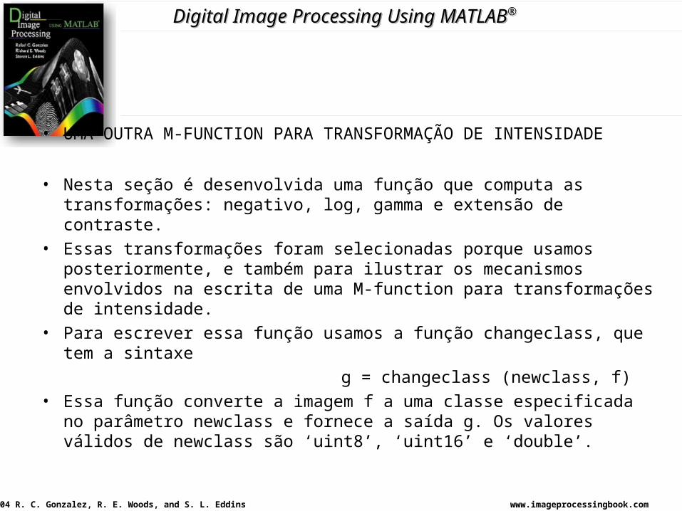
• UMA OUTRA M-FUNCTION PARA TRANSFORMAÇÃO DE INTENSIDADE
• Nesta seção é desenvolvida uma função que computa as transformações: negativo, log, gamma e extensão de contraste.
• Essas transformações foram selecionadas porque usamos posteriormente, e também para ilustrar os mecanismos envolvidos na escrita de uma M-function para transformações de intensidade.
• Para escrever essa função usamos a função changeclass, que tem a sintaxe g = changeclass (newclass, f)• Essa função converte a imagem f a uma classe especificada no parâmetro
newclass e fornece a saída g. Os valores válidos de newclass são ‘uint8’, ‘uint16’ e ‘double’.
www.imageprocessingbook.com© 2004 R. C. Gonzalez, R. E. Woods, and S. L. Eddins
Digital Image Processing Using MATLAB®
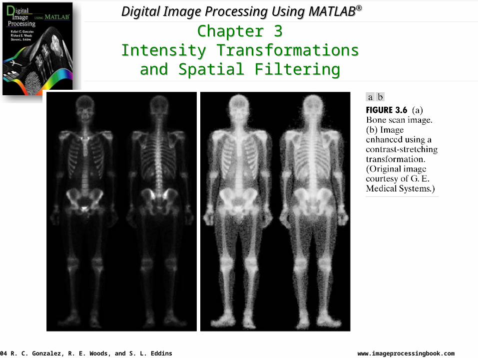
• Function g = intrans(f,varargin) (ver o código no livro)
• A Fig. 3.6b mostra o resultado do uso da função f = intrans (f,’stretch’, mean2(im2double(f)),0.9);
sobre a imagem da Fig. 3.6a.
www.imageprocessingbook.com© 2004 R. C. Gonzalez, R. E. Woods, and S. L. Eddins
Digital Image Processing Using MATLAB®
Chapter 3Intensity Transformations
and Spatial Filtering
www.imageprocessingbook.com© 2004 R. C. Gonzalez, R. E. Woods, and S. L. Eddins
Digital Image Processing Using MATLAB®
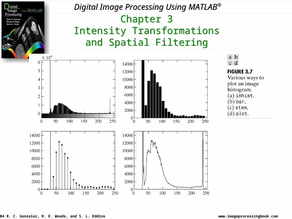
• PROCESSAMENTO DE HISTOGRAMA E PLOTAGEM DE FUNÇÃO• Geração de plotagem de histogramas de imagens:• A função para manipular histogramas é imhist, que tem a sintaxe h = imhist(f,b) onde b é o número de subdivisões na escala de intensidade. Se b é omitido, o valor default = 256.• O histograma normalizado pode ser obtido usando p = imhist(f,b)/numel(f)• Considerando a imagem da Fig. 3.3a, a forma mais simples de plotar o seu
histograma é: imhist(f);• A Fig. 3.7a mostra o resultado.
www.imageprocessingbook.com© 2004 R. C. Gonzalez, R. E. Woods, and S. L. Eddins
Digital Image Processing Using MATLAB®
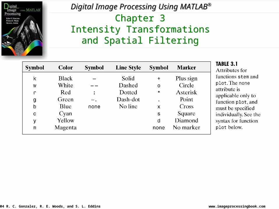
• Os histogramas são também plotadas em bar graphs. Para tanto devemos usar a função: bar (horz, v, width)
• Onde v é um vetor linha contendo os pontos a serem plotados, horz é um vetor de mesma dimensão que contem os incrementos na escala horizontal, e width é um número entre 0 e 1.
• Se horiz é omitido, o eixo horizontal é dividido em unidade de 0 a length(v).• Quando width é 1, as barras se tocam; quando é zero, as barras são apenas
linhas verticais, como na Fig. 3.7a. O valor default é 0.8.• Quando o bar graph é usado, reduz a resolução horizontal dividindo em
intervalos.
www.imageprocessingbook.com© 2004 R. C. Gonzalez, R. E. Woods, and S. L. Eddins
Digital Image Processing Using MATLAB®
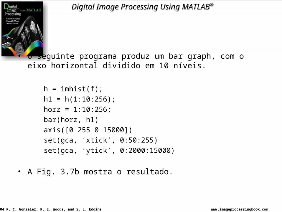
• O seguinte programa produz um bar graph, com o eixo horizontal dividido em 10 níveis.
h = imhist(f); h1 = h(1:10:256); horz = 1:10:256; bar(horz, h1) axis([0 255 0 15000]) set(gca, ‘xtick’, 0:50:255) set(gca, ‘ytick’, 0:2000:15000)
• A Fig. 3.7b mostra o resultado.
www.imageprocessingbook.com© 2004 R. C. Gonzalez, R. E. Woods, and S. L. Eddins
Digital Image Processing Using MATLAB®
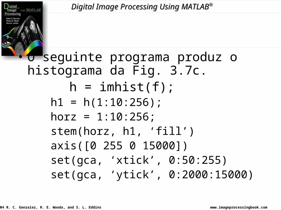
• O seguinte programa produz o histograma da Fig. 3.7c.
h = imhist(f); h1 = h(1:10:256); horz = 1:10:256; stem(horz, h1, ‘fill’) axis([0 255 0 15000]) set(gca, ‘xtick’, 0:50:255) set(gca, ‘ytick’, 0:2000:15000)
www.imageprocessingbook.com© 2004 R. C. Gonzalez, R. E. Woods, and S. L. Eddins
Digital Image Processing Using MATLAB®
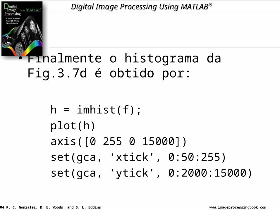
• Finalmente o histograma da Fig.3.7d é obtido por:
h = imhist(f); plot(h) axis([0 255 0 15000]) set(gca, ‘xtick’, 0:50:255) set(gca, ‘ytick’, 0:2000:15000)
www.imageprocessingbook.com© 2004 R. C. Gonzalez, R. E. Woods, and S. L. Eddins
Digital Image Processing Using MATLAB®
Chapter 3Intensity Transformations
and Spatial Filtering
www.imageprocessingbook.com© 2004 R. C. Gonzalez, R. E. Woods, and S. L. Eddins
Digital Image Processing Using MATLAB®
Chapter 3Intensity Transformations
and Spatial Filtering

www.imageprocessingbook.com© 2004 R. C. Gonzalez, R. E. Woods, and S. L. Eddins
Digital Image Processing Using MATLAB®
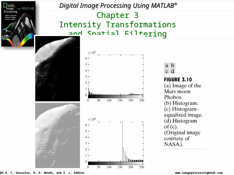
• EQUALIZAÇÃO DE HISTOGRAMA
• A equalização de histograma é implementada usando a função histeq, com a sintaxe
g = histeq(f, nlev) onde nlev é o número de níveis de intensidade especificado para a imagem
de saída.• Se nlev é igual a L (número total de possíveis níveis), o histeq implementa
a função de transformação, T (rk), diretamente.• Se nlev é menor que L, histeq tenta distribuir os níveis tal que eles se
aproximem de um histograma achatado (flat).• O valor default de nlev é 64.

www.imageprocessingbook.com© 2004 R. C. Gonzalez, R. E. Woods, and S. L. Eddins
Digital Image Processing Using MATLAB®
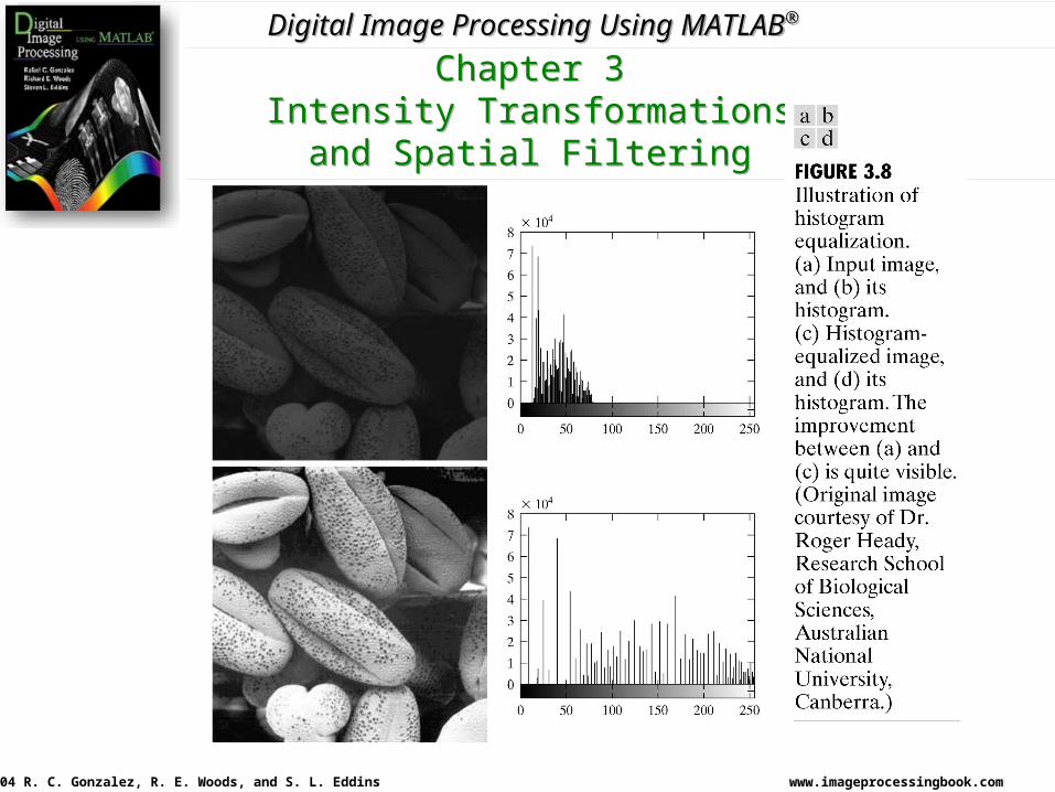
• A Fig. 3.8 mostra o resultado da aplicação da equalização de histograma, passo a passo, usando o seguinte programa:
imshow(f) figure, imhist(f) ylim (‘auto’) g = histeq (f, 256); figure, imshow (g) figure, imhist (g) ylim(‘auto’)
www.imageprocessingbook.com© 2004 R. C. Gonzalez, R. E. Woods, and S. L. Eddins
Digital Image Processing Using MATLAB®
Chapter 3Intensity Transformations
and Spatial Filtering

www.imageprocessingbook.com© 2004 R. C. Gonzalez, R. E. Woods, and S. L. Eddins
Digital Image Processing Using MATLAB®
Chapter 3Intensity Transformations
and Spatial Filtering

www.imageprocessingbook.com© 2004 R. C. Gonzalez, R. E. Woods, and S. L. Eddins
Digital Image Processing Using MATLAB®
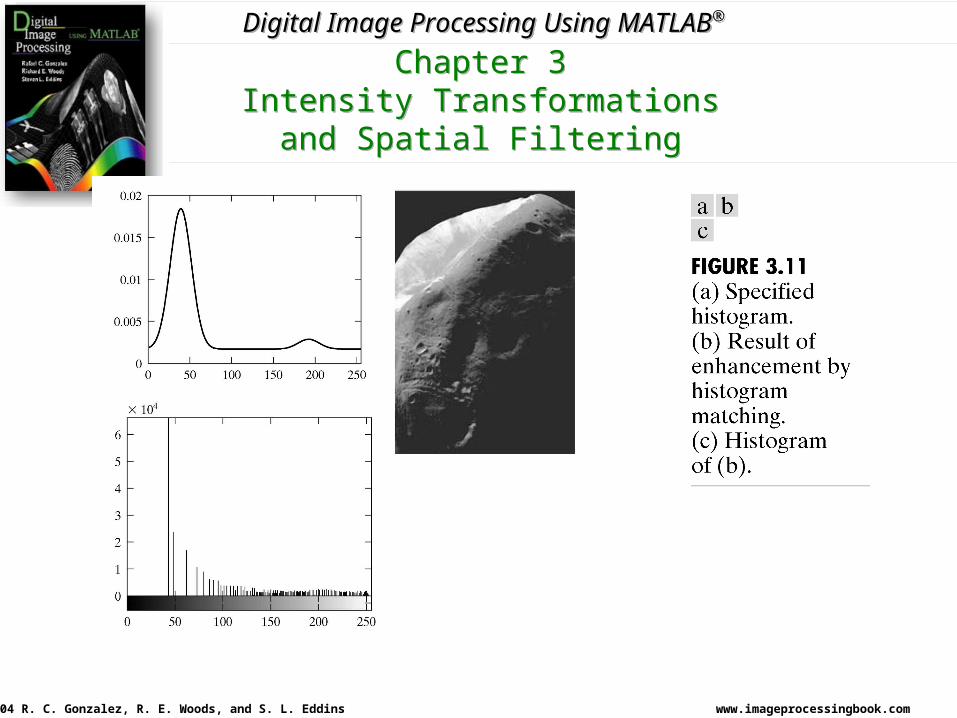
• ESPECIFICAÇÃO DE HISTOGRAMA
• O seguinte comando implementa a especificação de histograma
• g = histeq(f, hspec)
• onde hspec é o histograma especificado ( um vetor linha de valores especificados).
www.imageprocessingbook.com© 2004 R. C. Gonzalez, R. E. Woods, and S. L. Eddins
Digital Image Processing Using MATLAB®
Chapter 3Intensity Transformations
and Spatial Filtering
www.imageprocessingbook.com© 2004 R. C. Gonzalez, R. E. Woods, and S. L. Eddins
Digital Image Processing Using MATLAB®
Chapter 3Intensity Transformations
and Spatial Filtering
www.imageprocessingbook.com© 2004 R. C. Gonzalez, R. E. Woods, and S. L. Eddins
Digital Image Processing Using MATLAB®
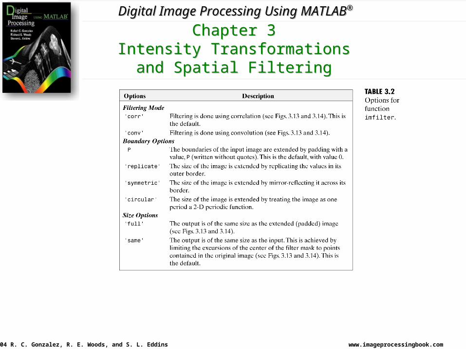
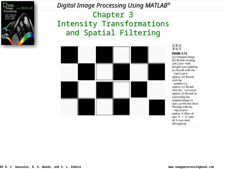
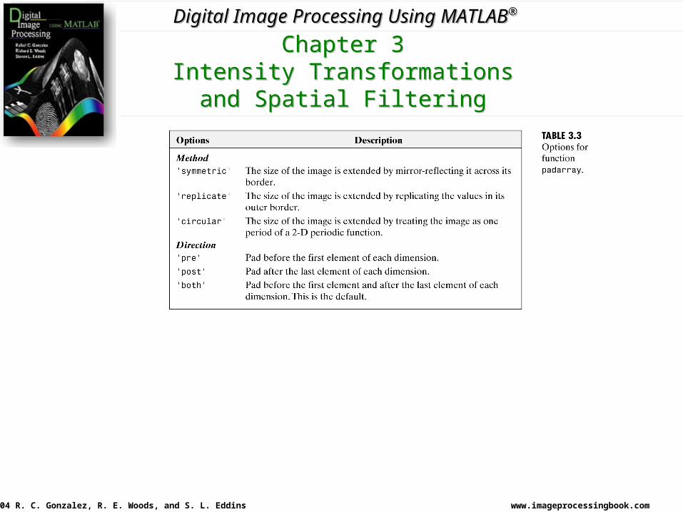
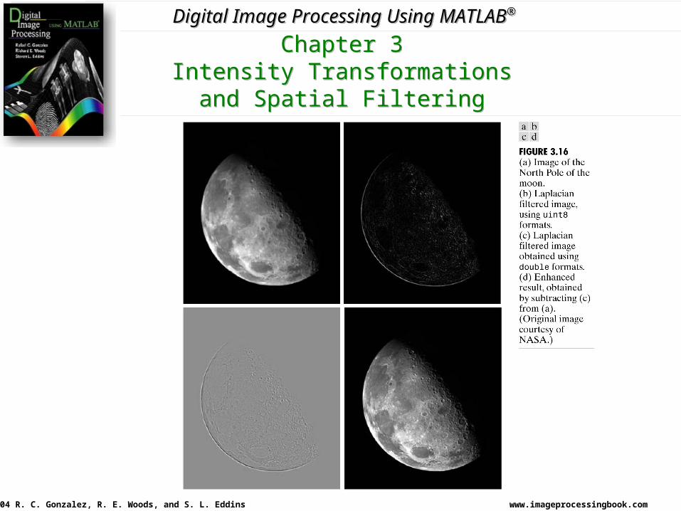
• FILTRAGEM ESPACIAL
www.imageprocessingbook.com© 2004 R. C. Gonzalez, R. E. Woods, and S. L. Eddins
Digital Image Processing Using MATLAB®
Chapter 3Intensity Transformations
and Spatial Filtering
www.imageprocessingbook.com© 2004 R. C. Gonzalez, R. E. Woods, and S. L. Eddins
Digital Image Processing Using MATLAB®
Chapter 3Intensity Transformations
and Spatial Filtering
www.imageprocessingbook.com© 2004 R. C. Gonzalez, R. E. Woods, and S. L. Eddins
Digital Image Processing Using MATLAB®
Chapter 3Intensity Transformations
and Spatial Filtering
www.imageprocessingbook.com© 2004 R. C. Gonzalez, R. E. Woods, and S. L. Eddins
Digital Image Processing Using MATLAB®
Chapter 3Intensity Transformations
and Spatial Filtering
www.imageprocessingbook.com© 2004 R. C. Gonzalez, R. E. Woods, and S. L. Eddins
Digital Image Processing Using MATLAB®
Chapter 3Intensity Transformations
and Spatial Filtering
www.imageprocessingbook.com© 2004 R. C. Gonzalez, R. E. Woods, and S. L. Eddins
Digital Image Processing Using MATLAB®
Chapter 3Intensity Transformations
and Spatial Filtering

www.imageprocessingbook.com© 2004 R. C. Gonzalez, R. E. Woods, and S. L. Eddins
Digital Image Processing Using MATLAB®
Chapter 3Intensity Transformations
and Spatial Filtering
www.imageprocessingbook.com© 2004 R. C. Gonzalez, R. E. Woods, and S. L. Eddins
Digital Image Processing Using MATLAB®
Chapter 3Intensity Transformations
and Spatial Filtering

www.imageprocessingbook.com© 2004 R. C. Gonzalez, R. E. Woods, and S. L. Eddins
Digital Image Processing Using MATLAB®
Chapter 3Intensity Transformations
and Spatial Filtering

www.imageprocessingbook.com© 2004 R. C. Gonzalez, R. E. Woods, and S. L. Eddins
Digital Image Processing Using MATLAB®
Chapter 3Intensity Transformations
and Spatial Filtering
Related Documents