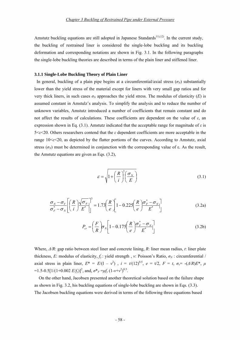
Chapter 3 Buckling of Restrained Pipe under External Pressure - 57 - Chapter 3 Buckling of Restrained Pipe under External Pressure The buckling of uniformly supported steel liner used in separated tunnel structure had been studied as a free pipe buckling and the corresponding theory solution were given. However, when the steel liner is installed with locally support in tunnel, the contact between tunnel lining and steel liner should be taken into account, as well as the restraining effects due to RC linings, because the critical pressure increases significantly for an elastic liner encased in rigid cavity when consider the restraining effect. In this chapter, the steel liner as restrained pipe, its buckling is investigated using experimental, numerical and analytical method, in terms of plain steel liner and stiffened liner. Meanwhile the corresponding theoretical solutions will be discussed, based on the existing single-lobe buckling theories. 3.1 Literature Review The buckling of encased cylindrical shells under external pressure has been studied since the mid-twentieth century. Two typical restrained hydrostatic buckling theories, the rotary symmetric buckling and the single-lobe buckling were presented by Borot, Vaughan, Cheney 1), 2) and Amstutz 3) , Jacobsen 4) , respectively. Because the single-lobe buckling theory had been verified by many practical buckling accidents, it is widely applied in the buckling analysis of encased cylindrical shells at present. The recent research works have been carried out by El-Sawy et al 5),6) , using numerical analysis, where Jacobsen theory was used to estimate the theoretical critical pressure. The other related studies were conducted by Croll 7) , Omara et al 8) , Yamamoto et al 9) , and etc. In addition, the Jacobsen buckling equations has been recommended by Berti, D. et al. 10) in the technical forum on buckling of tunnel liner under external pressure in 1998, because Jacobsen’s theory always gives conservative critical pressure. On the other hand, ρ R Δ β α R' Initial gap Tunnel lining (RC Segments) Steel liner Fig. 3.1 Schematic of single-lobe buckling

Welcome message from author
This document is posted to help you gain knowledge. Please leave a comment to let me know what you think about it! Share it to your friends and learn new things together.
Transcript

Chapter 3 Buckling of Restrained Pipe under External Pressure
- 57 -
Chapter 3 Buckling of Restrained Pipe under External Pressure
The buckling of uniformly supported steel liner used in separated tunnel structure had been studied as a free pipe buckling and the corresponding theory solution were given. However, when the steel liner is installed with locally support in tunnel, the contact between tunnel lining and steel liner should be taken into account, as well as the restraining effects due to RC linings, because the critical pressure increases significantly for an elastic liner encased in rigid cavity when consider the restraining effect. In this chapter, the steel liner as restrained pipe, its buckling is investigated using experimental, numerical and analytical method, in terms of plain steel liner and stiffened liner. Meanwhile the corresponding theoretical solutions will be discussed, based on the existing single-lobe buckling theories.
3.1 Literature Review The buckling of encased cylindrical shells under external pressure has been studied since
the mid-twentieth century. Two typical restrained hydrostatic buckling theories, the rotary symmetric buckling and the single-lobe buckling were presented by Borot, Vaughan, Cheney1),
2) and Amstutz3), Jacobsen 4), respectively. Because the single-lobe buckling theory had been verified by many practical buckling accidents, it is widely applied in the buckling analysis of encased cylindrical shells at present. The recent research works have been carried out by
El-Sawy et al 5),6), using numerical analysis, where Jacobsen theory was used to estimate the theoretical critical pressure. The other related studies were conducted by Croll7), Omara et al8), Yamamoto et al9), and etc. In addition, the Jacobsen buckling equations has been recommended by Berti, D. et al. 10) in the technical forum on buckling of tunnel liner under external pressure in 1998, because Jacobsen’s theory always gives conservative critical pressure. On the other hand,
ρ R
Δ
β
αR'
Initial gap
Tunnel lining(RC Segments)
Steel liner
Fig. 3.1 Schematic of single-lobe buckling
Chapter 3 Buckling of Restrained Pipe under External Pressure
- 58 -
Amstutz buckling equations are still adopted in Japanese Standards11),12). In the current study, the buckling of restrained liner is considered the single-lobe buckling and its buckling deformation and corresponding notations are shown in Fig. 3.1. In the following paragraphs the single-lobe buckling theories are described in terms of the plain liner and stiffened liner.
3.1.1 Single-Lobe Buckling Theory of Plain Liner
In general, buckling of a plain pipe begins at a circumferential/axial stress (σN) substantially lower than the yield stress of the material except for liners with very small gap ratios and for very thick liners, in such cases σN approaches the yield stress. The modulus of elasticity (E) is assumed constant in Amstulz’s analysis. To simplify the analysis and to reduce the number of unknown variables, Amstutz introduced a number of coefficients that remain constant and do not affect the results of calculations. These coefficients are dependent on the value of ε, an expression shown in Eq. (3.1). Amstutz indicated that the acceptable range for magnitude of ε is 5<ε<20. Others researchers contend that the ε dependent coefficients are more acceptable in the range 10<ε<20, as depicted by the flatter portions of the curves. According to Amstutz, axial stress (σN) must be determined in conjunction with the corresponding value of ε. As the result, the Amstutz equations are given as Eqs. (3.2),
⎟⎠⎞
⎜⎝⎛
⎟⎠⎞
⎜⎝⎛+=
EiR Nσε
2
1 (3.1)
⎥⎦
⎤⎢⎣
⎡ −⎟⎠⎞
⎜⎝⎛−⎟
⎠⎞
⎜⎝⎛=
⎥⎥⎦
⎤
⎢⎢⎣
⎡⎟⎠⎞
⎜⎝⎛
−−
*
*3
** 225.0173.1Ee
ReR
EiR NFN
NF
VN σσσσσσσ
(3.2a)
⎥⎦
⎤⎢⎣
⎡ −⎟⎠⎞
⎜⎝⎛−⎟
⎠⎞
⎜⎝⎛= *
*
175.01Ee
RRFP NF
Ncrσσσ (3.2b)
Where, Δ/R: gap ratio between steel liner and concrete lining, R: liner mean radius, t: liner plate thickness, E: modulus of elasticity, fy : yield strength , v: Poisson’s Ratio, σN : circumferential / axial stress in plain liner, E* = E/(l – v2) , i = t/(12)0.5, e = t/2, F = t, σv= -(Δ/R)E*, μ =1.5-0.5[1/(1+0.002 E/fy)]2, and, σ*F =μfy (1-v+v2)0.5.
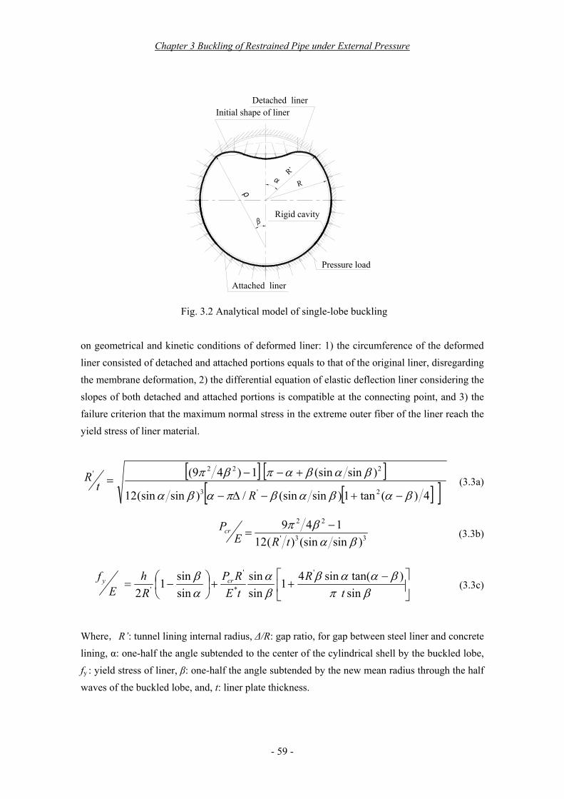
On the other hand, Jacobsen presented another theoretical solution based on the failure shape as shown in Fig. 3.2, his buckling equations of single-lobe buckling are shown in Eqs. (3.3). The Jacobsen buckling equations were derived in terms of the following three equations based
Chapter 3 Buckling of Restrained Pipe under External Pressure
- 59 -
α
β
Attached liner
Initial shape of liner Detached liner
Rigid cavity
Pressure load
R'
R
ρ
Fig. 3.2 Analytical model of single-lobe buckling
on geometrical and kinetic conditions of deformed liner: 1) the circumference of the deformed liner consisted of detached and attached portions equals to that of the original liner, disregarding the membrane deformation, 2) the differential equation of elastic deflection liner considering the slopes of both detached and attached portions is compatible at the connecting point, and 3) the failure criterion that the maximum normal stress in the extreme outer fiber of the liner reach the yield stress of liner material.
[ ] [ ][ ][ ]4)(tan1)sinsin(/)sinsin(12
)sinsin(1)49(2'3
222'
βαβαβπαβα
βαβαπβπ
−+−Δ−
+−−=
Rt
R (3.3a)
33'
22
)sinsin()(12149
βαβπ
tREPcr −
= (3.3b)
⎥⎦
⎤⎢⎣
⎡ −++⎟
⎠⎞
⎜⎝⎛ −=
βπβααβ
βα
αβ
sin)tan(sin41
sinsin
sinsin1
2
'
*
'
' tR
tERP
Rh
Ef cry (3.3c)
Where,R’: tunnel lining internal radius, Δ/R: gap ratio, for gap between steel liner and concrete lining, α: one-half the angle subtended to the center of the cylindrical shell by the buckled lobe, fy : yield stress of liner, β: one-half the angle subtended by the new mean radius through the half waves of the buckled lobe, and, t: liner plate thickness.
Chapter 3 Buckling of Restrained Pipe under External Pressure
- 60 -
3.1.2 Single-Lobe Buckling Theory of Stiffened Liners For ring-stiffened pipe, Amstutz presented an analytical solution in terms of buckling of
overall stiffened pipe and buckling of inter-stiffeners pipe. The theoretical analysis for general buckling was presented using the same equations of plain pipe mentioned above. However, the cross-sectional properties J, i, and e is defined as the cross-section of stiffener with a co-operating strip of the pipe shell with effective width of thirty times the thickness. For F, the overall cross-section including the pipe shell between stiffeners is taken. As the inter-stiffeners shell buckling, the buckling theory of free pipe was adopted using Flügge’s equations, because the inter-stiffeners shell was considered to be left off the rigid wall in the reach of the buckling wave.
In many literatures, that Amstutz analysis is not applicable to steel liners with stiffeners has been mentioned because it is limited to buckling with ε greater than 5, α less than 90°. Because of this reason, only Jacobsen’s analysis of single-lobe failure of a stiffened liner is adopted in many manual, and the Amstutz analysis is not recommended. Jacobsen’s analysis of steel liners with external stiffeners is similar to that without stiffeners, except that the stiffeners are computed for the total moment of inertia as the moment of inertia of the stiffener with contributing width of the shell equal to 1.57( Rt)0.5 + tr. As same with the case of un-stiffened liner, the analysis of stiffened liner is based on the assumption of a single-lobe failure. The three simultaneous equations with three unknown α, β, and Pcr are:
[ ] [ ][ ][ ]4)(tan1)sinsin(/)sinsin(12
)sinsin(1)49(12 2'3
222'
βαβαβπαβα
βαβαπβπ
−+−Δ−
+−−=
RFJR (3.4a)
33'
22
)sinsin()12(1214912
βαβπ
FJREFFJSPcr −
= (3.4b)
⎥⎦
⎤⎢⎣
⎡ −++⎟
⎠⎞
⎜⎝⎛ −=
βπβααβ
βα
αβ
sin3)tan(sin21
sinsin
sinsin1
''
' JFhR
EFSRP
Rh
Ef cry (3.4c)
Where, F: cross-sectional area of the stiffener and the pipe shell between the stiffeners, h: distance from neutral axis of stiffener to the outer edge of the stiffener, Pcr: critical external buckling pressure, and, J: moment of inertia of the stiffener and contributing width of the shell.
Chapter 3 Buckling of Restrained Pipe under External Pressure
- 61 -
3.1.3 Other Buckling Theories of Restrained Liner As well known, the critical pressure increases significantly for an elastic liner encased in rigid
cavity. Glock in 1977 analyzed the elastic stability problem of the constrained liner under external pressure, using a non-linear deformation theory and the principle of minimum potential energy to develop his solution based on a pre-assumption of the deformed shape of the detached part of the liner13). His solution can be written as
2.2
21⎟⎠⎞
⎜⎝⎛
−=
DtEPcr ν
(3.5)
The Glock solution was later extended by Boot14), 15) in 1998 to consider the effect of a gap between the liner and its host on the liner’s buckling pressure. Boot extended Glock.s closed-analysis theory to take account of initial gap imperfections and also to reflect the observed two-lobe buckling mode. Since then, the theories of Glock and Boot are usually called Boot-Glock theory. The generalized buckling equation derived by Boot can be expressed in convenient dimensionless form simply as Eq. (3.6) when converted to plane strain conditions for long pipe.
mcrcr
DtC
EP
EP −
⎟⎠⎞
⎜⎝⎛=
−=
)1( 2* ν (3.6)
Where, both the coefficient C and the power m of t/D are functions of imperfections in the focused system. For zero imperfection m = -2.2, and the coefficient C has value of 1.003 for single-lobe buckling corresponding to Glock’s published solution and 1.323 for two-lobe buckling. As the mean gap to radius ratio w/R increases, both m and C increase, and at very large gaps approach 2-lobe values of -3 and 2 respectively, corresponding to the unrestrained buckling formula.
The concept of comparing the buckling pressure between free and encased liner has been employed by both researchers and developers of design codes. The idea has been used to determine an enhancement factor K, which is used to define the critical pressure for the encased liner. The enhancement factor K was defined by Aggarwall and Cooper 16)as,
crr
cr KPP = (3.7)
Where,
3
212
⎟⎠⎞
⎜⎝⎛
−=
DtEPcr ν
The enhancement factor reflects the difference between the results by experiment and theory.
Chapter 3 Buckling of Restrained Pipe under External Pressure
- 62 -
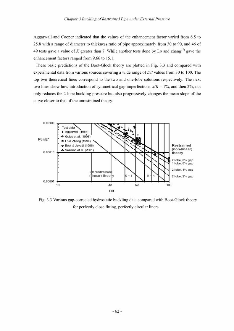
Aggarwall and Cooper indicated that the values of the enhancement factor varied from 6.5 to 25.8 with a range of diameter to thickness ratio of pipe approximately from 30 to 90, and 46 of 49 tests gave a value of K greater than 7. While another tests done by Lo and zhang17) gave the enhancement factors ranged from 9.66 to 15.1.
These basic predictions of the Boot-Glock theory are plotted in Fig. 3.3 and compared with experimental data from various sources covering a wide range of D/t values from 30 to 100. The top two theoretical lines correspond to the two and one-lobe solutions respectively. The next two lines show how introduction of symmetrical gap imperfections w/R = 1%, and then 2%, not only reduces the 2-lobe buckling pressure but also progressively changes the mean slope of the curve closer to that of the unrestrained theory.
Fig. 3.3 Various gap-corrected hydrostatic buckling data compared with Boot-Glock theory for perfectly close fitting, perfectly circular liners
Chapter 3 Buckling of Restrained Pipe under External Pressure
- 63 -
3.2 Contact Analysis Technology18)
Since a restrained liner will forms a detached part and attached another part during fitting the void between liner and its host, and the failure only occurs at a detached part of liner, the numerical analysis of buckling of restrained liner is required to simulate the contact phenomena. The contact analysis therefore, becomes the key issue to the analysis work. In the following paragraphs, the existing high-technology on numerical contact analysis is introduced with respect to the FEM software of MSC.Marc.
3.2.1 General Introduction With the numerical analysis technology development, the simulation of many physical
problems requires the ability to model the contact phenomena. This includes analyses of interference fits, rubber seals, tires, crash, and manufacturing processes among others. The analysis of contact behavior is complex due to the requirement to accurately track the motion of multiple geometric bodies, and the motion due to the interaction of these bodies after contact occurs. This includes representing the friction between surfaces and heat transfer between the bodies if required. The numerical objective is to detect the motion of the bodies, apply a constraint to avoid penetration, and apply appropriate boundary conditions to simulate the frictional behavior and heat transfer. Several procedures have been developed to treat these problems including the use of Perturbed or Augmented Lagrangian methods, penalty methods, and direct constraints. Furthermore, contact simulation has often required the use of special contact or gap elements. In many developed FEM software the contact analysis is allowed to be performed automatically without the use of special contact elements.
3.2.2 Contact Bodies Definition In contact analysis, there are two types of contact bodies deformable and rigid body required to
be defined. As the deformable body, there are three key aspects to be considered: 1) the elements which
make up the body, 2) the nodes on the external surfaces which might contact another body or itself, are treated as potential contact nodes, and, 3) the edges (2-D) or faces (3-D) which describe the outer surface in which a node on another body (or the same body) might contact, are treated as potential contact segments. Note that a body can be multiply connected (have holes in itself). It is also possible for a body to be composed of both triangular elements and quadrilateral elements in 2-D models or tetrahedral elements and brick elements in 3-D models. Beam elements and shells are also available for contact. However, it should not mix continuum elements, shells, and/or beams in a same contact body. Each node and element should be in, usually, one body. The elements in a body are defined using the CONTACT option. It is not
Chapter 3 Buckling of Restrained Pipe under External Pressure
- 64 -
necessary to identify the nodes on the exterior surfaces as this is done automatically. The algorithm used is based on the fact that nodes on the boundary are on element edges or faces that belong to only one element. Each node on the exterior surface is treated as a potential contact node. The potential deformable segments composed of edges or faces are treated in potentially two ways. The default is that they are considered as piece-wise linear (PWL). As an alternative, a cubic spline (2-D) or a Coons surface (3-D) can be placed through them. The SPLINE option is used to activate this procedure. This improves the accuracy of regular calculation.
Rigid bodies are composed of curves (2-D) or surfaces (3-D) or meshes with only thermal elements in coupled problems. The most significant aspect of rigid bodies is that they do not deform. Deformable bodies can contact rigid bodies, but contact between rigid bodies is not considered. In 3-D, a too large number is automatically reduced so that the analysis cost is not influenced too much. The treatment of the rigid bodies as NURBS surfaces is advantageous because it leads to a greater accuracy in the representation of the geometry and a more accurate calculation of the surface normal. Additionally, the variation of the surface normal is continuous over the body which leads to a better calculation of the friction behavior and a better convergence. To create a rigid body, one can either read in the curve and surface geometry created from a CAD system or create the geometry using MSC.Marc Mentat or directly enter it in MSC.Marc. The CONTACT option then can be used to select which geometric entities is to be a part of the rigid body. However, an important consideration for a rigid body is the definition of the interior side and the exterior side. It is not necessary for rigid bodies to define the complete body because only the bounding surface needs to be specified.
A CONTACT TABLE option or history definition option can be used to modify the order in which contact is established. This order can be directly user-defined or decided by the program. In the latter case, the order is based on the rule that if two deformable bodies might come into contact, searching is done such that the contacting nodes are on the body having the smallest element edge length and the contacted segments are on the body having the coarser mesh. It should be noted that this implies single-sided contact for this body combination, as opposed to the default double-sided contact.
3.2.3 Analysis Procedure and Parameters Analysis Procedure
In contact analysis a potential numerical procedure to simulate these complex contact problems has been implemented. At the beginning of the analysis, bodies should either be separated from one another or in contact. Bodies should not penetrate one another unless the objective is to perform an interference fit calculation. In practice, rigid body profiles are often complex, making it difficult to determine exactly where the first contact is located. Before the analysis
Chapter 3 Buckling of Restrained Pipe under External Pressure
- 65 -
begins (increment zero), if a rigid body has a nonzero motion associated with it, the initialization procedure brings it into first contact with a deformable body. No motion or distortion occurs in the deformable bodies during this process. The CONTACT TABLE option may be used to specify that the initial contact should be stress free. In such cases, the coordinates of the nodes are relocated on the surface so that initial stresses do not occur. During the incremental procedure, each potential contact node is first checked to see whether it is near a contact segment. The contact segments are either edges of other 2-D deformable bodies, faces of 3-D deformable bodies, or segments from rigid bodies. By default, each node could contact any other segment including segments on the body that it belongs to. This allows a body to contact itself. To simplify the computation, it is possible to use the CONTACT TABLE option to indicate that a particular body will or will not contact another body. This is often used to indicate that a body will not contact itself. During the iteration process, the motion of the node is checked to see whether it has penetrated a surface by determining whether it has crossed a segment. Because there can be a large number of nodes and segments, efficient algorithms have been developed to accelerate this process. A bounding box algorithm is used so that it is quickly determined whether a node is near a segment. If the node falls within the bounding box, more sophisticated techniques are used to determine the exact status of the node.
Contact Tolerance The contact tolerance is a vital quantity in contact analysis, which is used to judge whether the
contact happen. When a node is within the contact tolerance, it is considered to be in contact with the segment. The value of the contact tolerance has a significant impact on the computational time and the accuracy of the solution. In default, the contact tolerance is calculated by the program as the smaller value of 5% of the smallest element length or 25% of the smallest (beam or shell) element thickness. It is also possible to define the contact tolerance by inputting its value directly. If the contact tolerance is too small, detection of contact and penetration is difficult which leads to long computation time. Penetration of a node happens in a shorter time period leading to more repetition due to iterative penetration checking or to more increment splitting and increases the computational costs. If the contact tolerance is too large, nodes are considered in contact prematurely, resulting in a loss of accuracy or more repetition due to separation. Furthermore, the accepted solution might have nodes that “penetrate” the surface less than the error tolerance, but more desirable to the user. The default error tolerance is recommended. Usually, there are areas exist in the model where nodes are almost touching a surface. In such cases, the use of a biased tolerance area with a smaller distance on the outside and a larger distance on the inside is recommended. This avoids the close nodes from coming into contact and separating again and is accomplished by entering a bias factor. The bias factor should be given a value between 0.0 and 0.99. The default is 0.0 or no bias. Also, in analyses
Chapter 3 Buckling of Restrained Pipe under External Pressure
- 66 -
involving frictional contact, a bias factor for the contact tolerance is inside contact area (1 + bias) times the contact tolerance. The recommended value of bias factor is 0.95.
As for shell contact, it is considered shell contact occurred when the position of a node pulsing or minusing half the thickness projected with the normal comes into contact with another segment. As the shell has finite thickness, the node (depending on the direction of motion) can physically contact either the top surface, bottom surface, or mathematically contact can be based upon the mid-surface. One can control whether detection occurs with either / both surfaces, the top surface, the bottom surface, or the middle surface. In such cases, either two or one segment will be created at the appropriate physical location. Note that these segments will be dependent, not only on the motion of the shell, but also the current shell thickness.
Friction and Separation Friction is a complex physical phenomenon that involves the characteristics of the surface such
as surface roughness, temperature, normal stress, and relative velocity. An example of this complexity is that quite often in contact problems neutral lines develop. This means that along a contact surface, the material flows in one direction in part of the surface and in the opposite direction in another part of the surface. Such neutral lines are, in general, not known a priori. The actual physics of friction and its numerical representation are continuously to be topics of research. Currently, in MSC.Marc the modeling of friction has basically been simplified to two idealistic models. The most popular friction model is the Coulomb friction model. This model is used for most applications with the exception of bulk forming as encountered in e.g. forging processes. For such applications the shear friction model is more appropriate.
In contact analysis, another physical phenomenon is separation. After a node comes into contact with a surface, it is possible to separate in a subsequent iteration or increment. Mathematically, a node should separate when the reaction force between the node and surface becomes tensile or positive. Physically, one could consider that a node should separate when the tensile force or normal stress exceeds the surface tension. Rather than use an exact mathematical definition, one can enter the force or stress required to cause separation. Separation can be based upon either the nodal forces or the nodal stresses. The use of the nodal stress method is recommended as the influence of element size is eliminated. When using higher-order elements and true quadratic contact, the separation criteria must be based upon the stresses as the equivalent nodal forces oscillate between the corner and mid-side nodes.
However, in many cases contact occurs but the contact forces are small; for example, laying a piece of paper on a desk. Because of the finite element procedure, this could result in numerical chattering. MSC.Marc has some additional contact control parameters that can be used to minimize this problem. As separation results in additional iterations (which leads to higher costs), the appropriate choice of parameters can be very beneficial. When contact occurs, a
Chapter 3 Buckling of Restrained Pipe under External Pressure
- 67 -
reaction force associated with the node in contact balances the internal stress of the elements adjacent to this node. When separation occurs, this reaction force behaves as a residual force (as the force on a free node should be zero). This requires that the internal stresses in the deformable body are redistributed. Depending on the magnitude of the force, this might require several iterations. You should note that in static analysis, if a deformable body is constrained only by other bodies (no explicit boundary conditions) and the body subsequently separates from all other bodies, it would then have rigid body motion. For static analysis, this would result in a singular or non-positive definite system. This problem can be avoided by setting appropriate boundary conditions. A special case of separation is the intentional release of all nodes from a rigid body.
Chapter 3 Buckling of Restrained Pipe under External Pressure
- 68 -
3.3 Pre-Discussions on Buckling of Restrained Liner
The analysis of restrained hydrostatic buckling is more complex than the free hydrostatic buckling of liner, because the buckling location in the former analysis has to be predicted except the critical pressure. On the other hand, as the application of existing buckling equations, Jacobsen equations can be physically applied directly, however, the application of Amstutz equations should satisfy the variation ε required in the range of 5 to 20. In the following paragraphes, the buckling location prediction and the application of theory equations will be given. Meanwhile, the methodology and the objective of the study on buckling of restrained liner will be discussed.
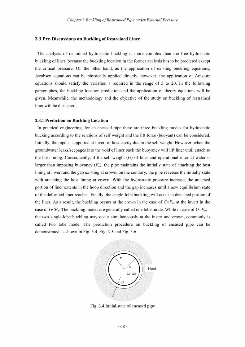
3.3.1 Prediction on Buckling Location In practical engineering, for an encased pipe there are three buckling modes for hydrostatic
bucking according to the relations of self weight and the lift force (buoyant) can be considered. Initially, the pipe is supported at invert of host cavity due to the self-weight. However, when the groundwater leaks/seepages into the void of liner back the buoyancy will lift liner until attach to the host lining. Consequently, if the self weight (G) of liner and operational internal water is larger than imposing buoyancy (Fb), the pipe maintains the initially state of attaching the host lining at invert and the gap existing at crown, on the contrary, the pipe reverses the initially state with attaching the host lining at crown. With the hydrostatic pressure increase, the attached portion of liner extents in the hoop direction and the gap increases until a new equilibrium state of the deformed liner reaches. Finally, the single-lobe buckling will occur in detached portion of the liner. As a result, the buckling occurs at the crown in the case of G>Fb, at the invert in the
case of G<Fb. The buckling modes are generally called one lobe mode. While in case of G=Fb,
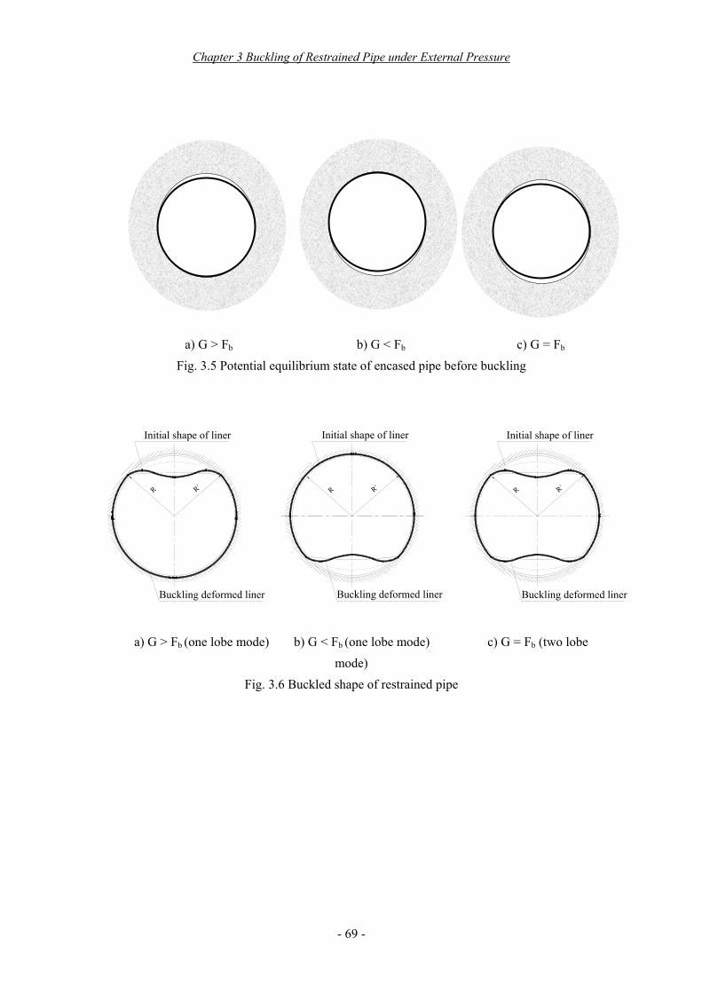
the two single-lobe buckling may occur simultaneously at the invert and crown, commonly is called two lobe mode. The prediction procedure on buckling of encased pipe can be demonstrated as shown in Fig. 3.4, Fig. 3.5 and Fig. 3.6.
Fig. 3.4 Initial state of encased pipe
R'
R
⊿
Host Liner
Chapter 3 Buckling of Restrained Pipe under External Pressure
- 69 -
a) G > Fb b) G < Fb c) G = Fb Fig. 3.5 Potential equilibrium state of encased pipe before buckling
R'
Buckling deformed liner
Initial shape of liner
R R'R R'R
Buckling deformed liner
Initial shape of liner
Buckling deformed liner
Initial shape of liner
a) G > Fb (one lobe mode) b) G < Fb (one lobe mode) c) G = Fb (two lobe mode)
Fig. 3.6 Buckled shape of restrained pipe
Chapter 3 Buckling of Restrained Pipe under External Pressure
- 70 -
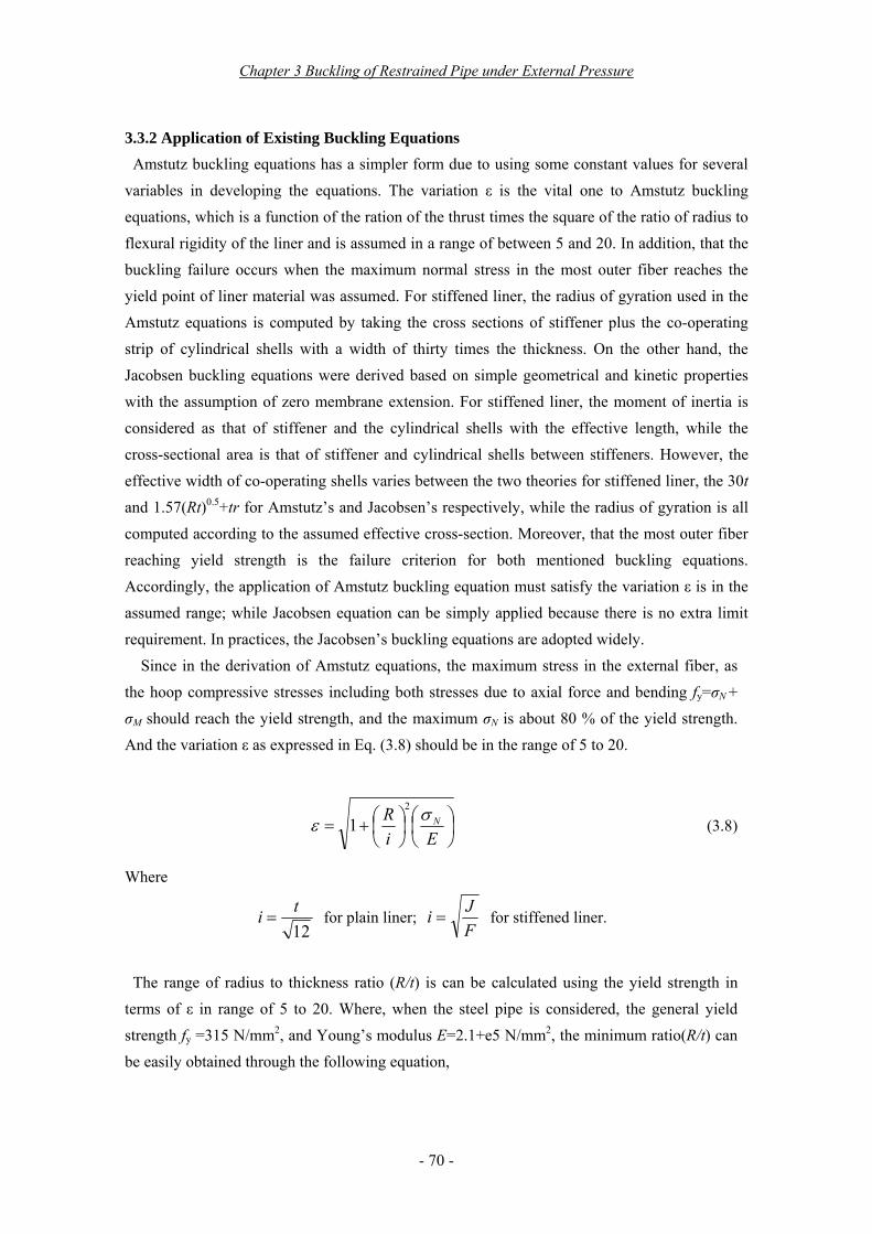
3.3.2 Application of Existing Buckling Equations Amstutz buckling equations has a simpler form due to using some constant values for several
variables in developing the equations. The variation ε is the vital one to Amstutz buckling equations, which is a function of the ration of the thrust times the square of the ratio of radius to flexural rigidity of the liner and is assumed in a range of between 5 and 20. In addition, that the buckling failure occurs when the maximum normal stress in the most outer fiber reaches the yield point of liner material was assumed. For stiffened liner, the radius of gyration used in the Amstutz equations is computed by taking the cross sections of stiffener plus the co-operating strip of cylindrical shells with a width of thirty times the thickness. On the other hand, the Jacobsen buckling equations were derived based on simple geometrical and kinetic properties with the assumption of zero membrane extension. For stiffened liner, the moment of inertia is considered as that of stiffener and the cylindrical shells with the effective length, while the cross-sectional area is that of stiffener and cylindrical shells between stiffeners. However, the effective width of co-operating shells varies between the two theories for stiffened liner, the 30t and 1.57(Rt)0.5+tr for Amstutz’s and Jacobsen’s respectively, while the radius of gyration is all computed according to the assumed effective cross-section. Moreover, that the most outer fiber reaching yield strength is the failure criterion for both mentioned buckling equations. Accordingly, the application of Amstutz buckling equation must satisfy the variation ε is in the assumed range; while Jacobsen equation can be simply applied because there is no extra limit requirement. In practices, the Jacobsen’s buckling equations are adopted widely.
Since in the derivation of Amstutz equations, the maximum stress in the external fiber, as the hoop compressive stresses including both stresses due to axial force and bending fy=σN + σM should reach the yield strength, and the maximum σN is about 80 % of the yield strength. And the variation ε as expressed in Eq. (3.8) should be in the range of 5 to 20.
⎟⎠⎞
⎜⎝⎛
⎟⎠⎞
⎜⎝⎛+=
EiR Nσε
2
1 (3.8)
Where
12ti = for plain liner;
FJi = for stiffened liner.
The range of radius to thickness ratio (R/t) is can be calculated using the yield strength in
terms of ε in range of 5 to 20. Where, when the steel pipe is considered, the general yield strength fy =315 N/mm2, and Young’s modulus E=2.1+e5 N/mm2, the minimum ratio(R/t) can be easily obtained through the following equation,
Chapter 3 Buckling of Restrained Pipe under External Pressure
- 71 -
yN fEE
tR
6.9)1(
12)1( 22 −≥
−=
εσ
ε )205( ≤≤ ε (3.9a)
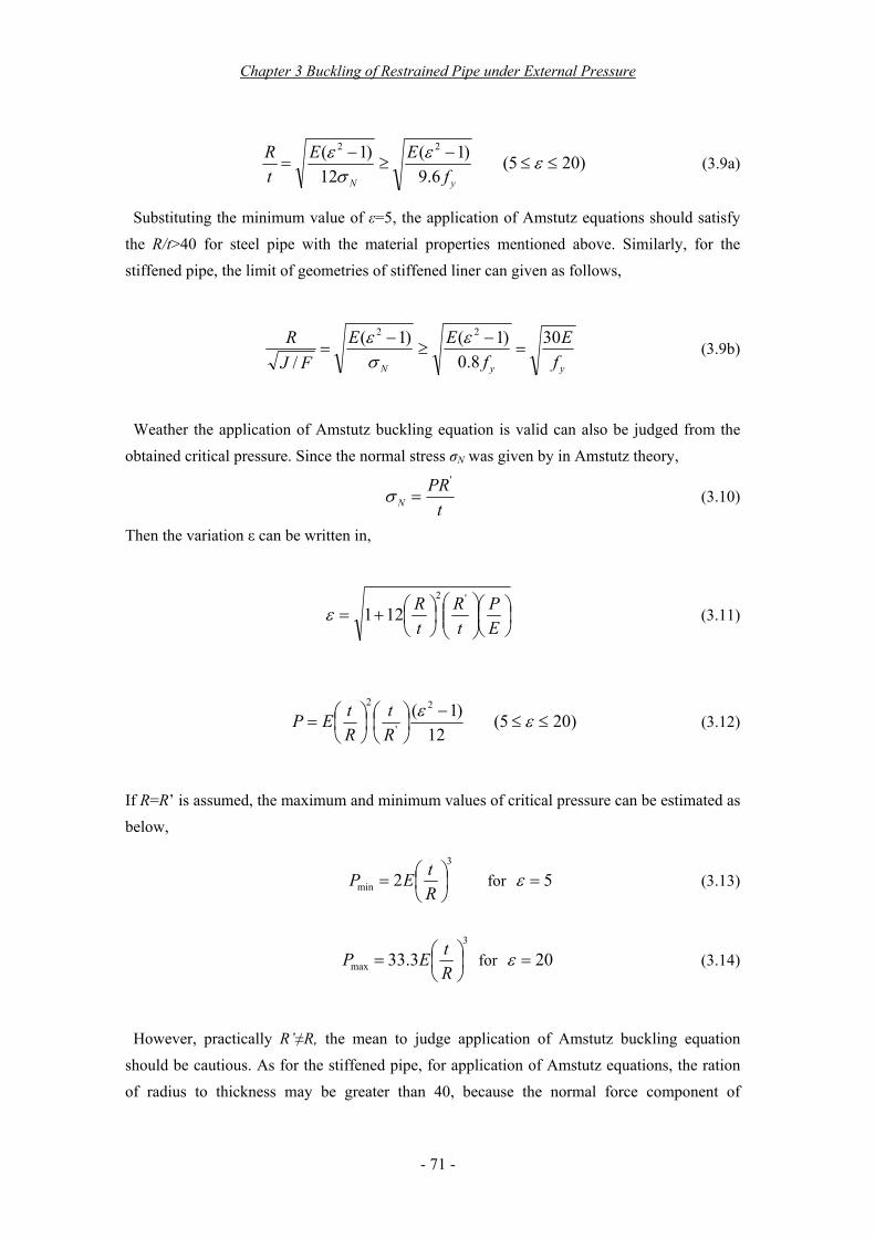
Substituting the minimum value of ε=5, the application of Amstutz equations should satisfy the R/t>40 for steel pipe with the material properties mentioned above. Similarly, for the stiffened pipe, the limit of geometries of stiffened liner can given as follows,
yyN fE
fEE
FJR 30
8.0)1()1(
/
22
=−
≥−
=ε
σε
(3.9b)
Weather the application of Amstutz buckling equation is valid can also be judged from the
obtained critical pressure. Since the normal stress σN was given by in Amstutz theory,
tPR
N
'
=σ (3.10)
Then the variation ε can be written in,
⎟⎠⎞
⎜⎝⎛⎟⎟⎠
⎞⎜⎜⎝
⎛⎟⎠⎞
⎜⎝⎛+=
EP
tR
tR '2
121ε (3.11)
12)1( 2
'
2 −⎟⎠⎞
⎜⎝⎛
⎟⎠⎞
⎜⎝⎛=
εRt
RtEP )205( ≤≤ ε (3.12)
If R=R’ is assumed, the maximum and minimum values of critical pressure can be estimated as below,
3
min 2 ⎟⎠⎞
⎜⎝⎛=
RtEP for 5=ε (3.13)
3
max 3.33 ⎟⎠⎞
⎜⎝⎛=
RtEP for 20=ε (3.14)
However, practically R’≠R, the mean to judge application of Amstutz buckling equation
should be cautious. As for the stiffened pipe, for application of Amstutz equations, the ration of radius to thickness may be greater than 40, because the normal force component of

Chapter 3 Buckling of Restrained Pipe under External Pressure
- 72 -
compressive stresses is smaller than the satisfactory providing σN <0.8 fy. On the other hand, although Jacobsen equations are widely recommended by many
researchers there is still a major criticism for the solution. The solution did not explicitly consider the elastic or inelastic stability of the liner but instead Jacobsen assumed that the ultimate pressure capacity of the liner corresponds to the first yielding at outer point in the liner. For a liner that buckles elastically before any material yielding (i.e. thin liner), this assumption is expected to overestimate the critical pressure since the pressure is controlled by the first yield of the liner. For the liners that yield before buckling (i.e. thick liners), the critical pressure values are expected to be underestimated since there is a considerable amount of pressure that can be carried by the liner after its first yield. This suggests that the Jacobsen solution should be critically evaluated. Moreover, although there is no limit requirement, the solution is difficult to solve out because it is consisted of three equations with too many unknown variants.
3.3.3 Methodology and Objective The investigation of buckling of restrained pipe should consider three cases in terms of G<Fb
G>Fb and G=Fb. As the approaching methods, the self weight loading is taken into account in the numerical analysis, as well as the buoyancy produced non-uniform hydrostatic water pressure. For the experimental investigation, since the single-lobe buckling occur in the portion of detached shells after equilibrium state reaches, and its behavior is almost identical to the bending behavior of a simple supported arch, the simplified model experiments are carried out using one half of un-stiffened and stiffened pipes. Where, the two liner loads are applied at the crown of test models to simulate the un-conservational hydrostatic pressure acting on the single-lobe deformed liner. As for the theoretical critical pressure calculation, the computing programs for Amstutz and Jacobsen equations are made using computer program language VB, respectively.
Considering the complexity of restrained hydrostatic buckling of liner installed in separated-type water tunnel, the investigations are mainly carried out in following aspects: 1) investigate the buckling behavior of restrained pipe and examine the existing two buckling theories, using numerical analysis method; 2) investigate the failure mechanism of single-lobe buckling and examine the existing two single-lobe buckling theories, using experimental analysis method; and, 3) discuss and present rational single-lobe buckling theories.
Chapter 3 Buckling of Restrained Pipe under External Pressure
- 73 -
3.4 Numerical Analysis of Buckling of Restrained Liner
3.4.1 Numerical Analysis Modeling Finite Element Analysis Modeling
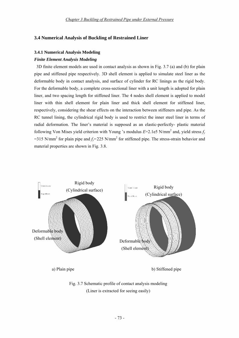
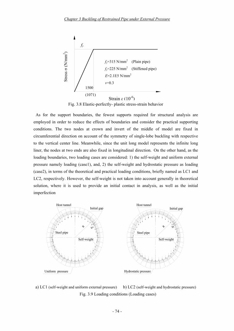
3D finite element models are used in contact analysis as shown in Fig. 3.7 (a) and (b) for plain pipe and stiffened pipe respectively. 3D shell element is applied to simulate steel liner as the deformable body in contact analysis, and surface of cylinder for RC linings as the rigid body. For the deformable body, a complete cross-sectional liner with a unit length is adopted for plain liner, and two spacing length for stiffened liner. The 4 nodes shell element is applied to model liner with thin shell element for plain liner and thick shell element for stiffened liner, respectively, considering the shear effects on the interaction between stiffeners and pipe. As the RC tunnel lining, the cylindrical rigid body is used to restrict the inner steel liner in terms of radial deformation. The liner’s material is supposed as an elastic-perfectly- plastic material following Von Mises yield criterion with Young ’s modulus E=2.1e5 N/mm2 and, yield stress fy =315 N/mm2 for plain pipe and fy=225 N/mm2 for stiffened pipe. The stress-strain behavior and material properties are shown in Fig. 3.8.
a) Plain pipe b) Stiffened pipe
Fig. 3.7 Schematic profile of contact analysis modeling (Liner is extracted for seeing easily)
Rigid body (Cylindrical surface)
Deformable body (Shell element)
Rigid body (Cylindrical surface)
Deformable body(Shell element)
Chapter 3 Buckling of Restrained Pipe under External Pressure
- 74 -
Steel pipe
Δ
Initial gap
Self-weight
R
Host tunnel
Uniform pressure Hydrostatic pressure
Steel pipe
Host tunnel
R
Self-weight
Initial gap
Δ
Fig. 3.8 Elastic-perfectly- plastic stress-strain behavior
As for the support boundaries, the fewest supports required for structural analysis are employed in order to reduce the effects of boundaries and consider the practical supporting conditions. The two nodes at crown and invert of the middle of model are fixed in circumferential direction on account of the symmetry of single-lobe buckling with respective to the vertical center line. Meanwhile, since the unit long model represents the infinite long liner, the nodes at two ends are also fixed in longitudinal direction. On the other hand, as the loading boundaries, two loading cases are considered: 1) the self-weight and uniform external pressure namely loading (case1), and, 2) the self-weight and hydrostatic pressure as loading (case2), in terms of the theoretical and practical loading conditions, briefly named as LC1 and LC2, respectively. However, the self-weight is not taken into account generally in theoretical solution, where it is used to provide an initial contact in analysis, as well as the initial imperfection
a) LC1 (self-weight and uniform external pressure) b) LC2 (self-weight and hydrostatic pressure)
Fig. 3.9 Loading conditions (Loading cases)
fy=315 N/mm2 (Plain pipe)
fy=225 N/mm2 (Stiffened pipe)
E=2.1E5 N/mm2
v=0.3 1500
(1071)
fy
Strain ε (10-6)
Stre
ss σ
(N/m
m2 )
Chapter 3 Buckling of Restrained Pipe under External Pressure
- 75 -
inevitably required for buckling analysis using arc-length increment method. Whereas the loading case2 (LC2), the practical loading conditions is completely simulated when the underground water leaks /seepages into water tunnel. In addition, the initial imperfections due to self-weight and uniform external pressure can also be taken into account. The two loading conditions are shown in Fig. 3.9, respectively.
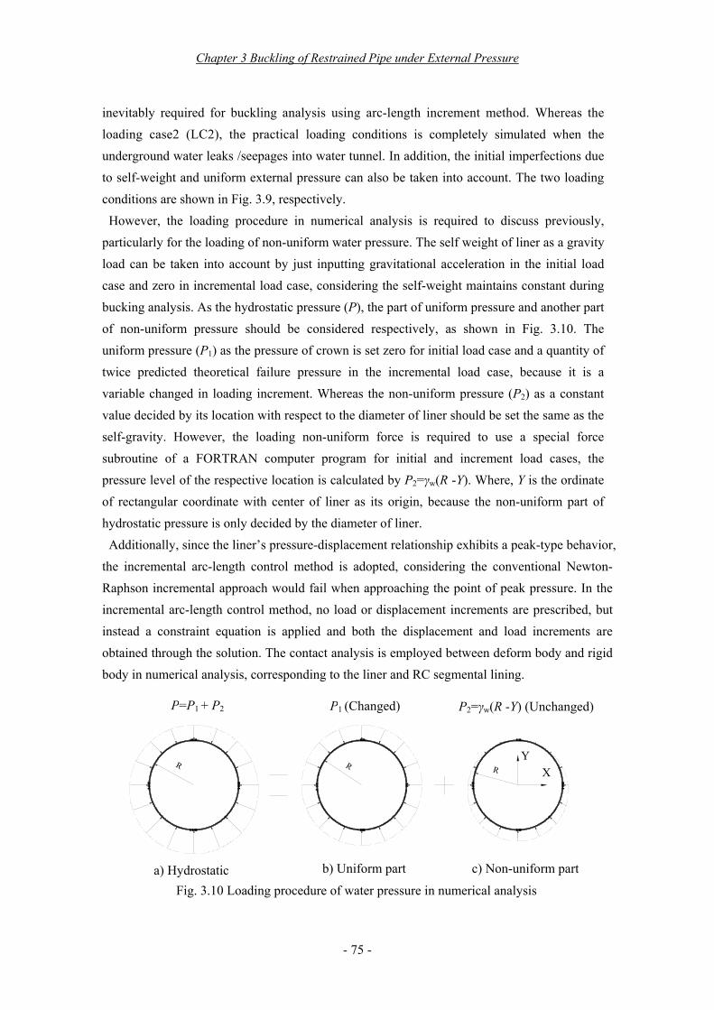
However, the loading procedure in numerical analysis is required to discuss previously, particularly for the loading of non-uniform water pressure. The self weight of liner as a gravity load can be taken into account by just inputting gravitational acceleration in the initial load case and zero in incremental load case, considering the self-weight maintains constant during bucking analysis. As the hydrostatic pressure (P), the part of uniform pressure and another part of non-uniform pressure should be considered respectively, as shown in Fig. 3.10. The uniform pressure (P1) as the pressure of crown is set zero for initial load case and a quantity of twice predicted theoretical failure pressure in the incremental load case, because it is a variable changed in loading increment. Whereas the non-uniform pressure (P2) as a constant value decided by its location with respect to the diameter of liner should be set the same as the self-gravity. However, the loading non-uniform force is required to use a special force subroutine of a FORTRAN computer program for initial and increment load cases, the pressure level of the respective location is calculated by P2=γw(R -Y). Where, Y is the ordinate of rectangular coordinate with center of liner as its origin, because the non-uniform part of hydrostatic pressure is only decided by the diameter of liner.
Additionally, since the liner’s pressure-displacement relationship exhibits a peak-type behavior, the incremental arc-length control method is adopted, considering the conventional Newton- Raphson incremental approach would fail when approaching the point of peak pressure. In the incremental arc-length control method, no load or displacement increments are prescribed, but instead a constraint equation is applied and both the displacement and load increments are obtained through the solution. The contact analysis is employed between deform body and rigid body in numerical analysis, corresponding to the liner and RC segmental lining.
Fig. 3.10 Loading procedure of water pressure in numerical analysis
R R R
a) Hydrostatic b) Uniform part c) Non-uniform part
P2=γw(R -Y) (Unchanged)P1 (Changed)P=P1 + P2
Y X
Chapter 3 Buckling of Restrained Pipe under External Pressure
- 76 -
Contact Analysis Setting RC tunnel lining and liner are modeled as a rigid body and a deformable body, respectively.
And the deformable body should be defined before rigid body. A contact table is also set by which the relationship between contact bodies in a contact analysis can be specified for the purposes:
・indicate which set of bodies may or may not touch each other, so that the computational time can be saved;
・define contact analysis inertias , like contact tolerance, bias factor; ・define different properties per set of contact bodies, like friction coefficient, error tolerance, and separation force. Where, the single side touching of deformable body touching rigid body is set, and an option is used to specify that the initial contact is stress free.
As discussed in section 3.2, the contact tolerance has a significant impact on the computational costs and the accuracy of the solution. If the contact tolerance is too small, detection of contact and penetration is difficult which leads to long computational time. Penetration of a node happens in a earlier time can lead to more repetitions due to iterative penetration checking or to more increment splitting and increases the computational time. In the contrast, if the contact tolerance is too large, nodes are considered in contact prematurely, resulting in a loss of accuracy or more repetition due to separation. Furthermore, the accepted solution might have nodes that “penetrate” the surface less than the error tolerance, but more than that desired by the user. Since the contact tolerance is dependent upon the value of error tolerance and bias factor, the error tolerance is carefully considered, as well the bias factor. In the current study, the error tolerance are set zero for plain pipe and 0.001 times height of stiffeners for stiffened pipe, considering the difference of practical contact phenomenon between plain pipe and stiffened pipe corresponding to the face and edge contacting. The contact happens when the node of pipe touch the surface of RC tunnel lining for plain liner, while when the node of stiffeners is below the tolerance distance for stiffened liner. It is therefore rational to adopt a larger size of error tolerance for stiffened liner considering the stiffened liner has small area of stiffener edge to detect the touching surface. Otherwise, at the default error tolerance of 25%, the smallest shell thickness varying with thickness is easy to induce the different contact criterion. Moreover, the large areas exist in the model where nodes are almost touching a surface during increment of loading. In such cases, the use of a biased tolerance area with a smaller distance on the outside and a larger distance on the inside is recommended. This avoids the close nodes from coming into contact and separating again and is accomplished by entering a bias factor. Also, in analyses involving frictional contact, a bias factor for the contact tolerance is inside contact area (1 + bias) times the error tolerance. Accordingly, by increasing the bias factor, the outside contact tolerance zone is decreased and the inside contact tolerance zone is increased. This generally reduces the number of iterations to get a converged solution. Where, the bias factor is
Chapter 3 Buckling of Restrained Pipe under External Pressure
- 77 -
set by using the recommended value 0.95. Additionally, the top surface check is set for plain liner by which nodes only come into contact
with top layer and ignore the thickness of shells. Whereas for stiffened liner, both the top and bottom surface check are set considering the nodes distributed on both bottom and top surface of stiffener is potential to contact. As the separation, it is considered that separation occurs when the contact normal stress on the node in contact becomes larger than the separation stress set as 0. In other words, when tensile is produced in contact normal stress, the separation occurs. In the current study, the friction during contact is disregarded, considering the friction factor between steel liner and the RC lining is rather smaller in water surrounding.

Chapter 3 Buckling of Restrained Pipe under External Pressure
- 78 -
3.4.2 Buckling of Plain Liner Analysis Models and Cases
The numerical analysis is carried out using 5 models with different ratio of radius to thickness, as shown in Table 3.1. In addition, for each model the 11 gap cases are considered in terms of the ranges of gap ratio from 0 to 20%, as shown in Table 3.2. Meanwhile, the Application range of Amstutz’s equations for computing critical pressure by means of Eq. (3.13) and Eq. (3.14) are summarized in Table 3.3. The vilification of Amstutz equation’s application is conducted
Table 3.1 Analysis models
Models Radius R (mm)
Thickness t (mm)
R/t
Model1 7.5 200.0 Model2 12 125.0 Model3 20 75.0 Model4 30 50.0 Model5
1500
42 35.7
Table 3.2 Gap cases
Cases Gap
⊿(mm)
R' (m)
Gap ratio
⊿/R (%)
1 1.5E-3 1.5 1.0E-042 0.6 1.5006 0.043 1.2 1.5012 0.084 3.0 1.503 0.15 7.5 1.5075 0.56 15.0 1.515 1.07 22.5 1.5225 1.58 30.0 1.53 2.09 37.5 1.5375 2.510 75.0 1.575 5.011 300 1.8 20.0
Table 3.3 Application range of Amstutz’s equation for computing critical pressure
Pcr (kN/m2) Model1 Model2 Model3 Model4 Model5
Max. 874 3580 16576 55944 153510
Min. 53 215 996 3360 9220

Chapter 3 Buckling of Restrained Pipe under External Pressure
- 79 -
through checking the obtained critical pressure: if the calculated critical pressure belongs to the range, the Amstutz’s equation can be judged to be applicable..
Moreover, in the current study the material density, ρs =7.8 t/m3 for the steel liner, and ρw
=1.0 t/m3 for the water are taken, respectively. For the loading case2 (LC2), taking into account the non-uniform water pressure, the buoyancy of unit length pipe (Fb) and the self-weight is (W) are calculated as follows,
Fb=πR2ρwg (3.15)
W=2πRtρsg (3.16)
By substituting ρw=1.0 t/m3 and ρs =7.8 t/m3 to above equations, the ratio of buoyancy to self weight can be obtained as,
Fb/W=Rρw/2tρs=R/15.6t (3.17)
According to the above discussion, the single-lobe bucking occurs at invert only when the buoyancy is larger than the self-weight, therefore in terms of the radius to thickness ratio, the single-lobe bucking occurs at invert for the model with the geometrics of R/t>15.6. From Table 3.1, the buckling failure should occur at invert for loading case2, because the radius to thickness ratios of all models are R/t>15.6. Whereas for the buckling under loading case1, the single-lobe buckling should occur at crown, since the acting loads are self-weight and uniform pressure without the buoyancy.
Numerical Analysis Results and Discussions
1) Single-lobe buckling mechanism The numerical analysis of all models is carried out for all the gap cases, and all the results are
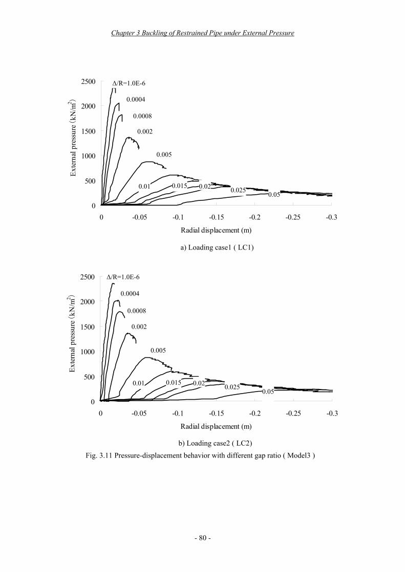
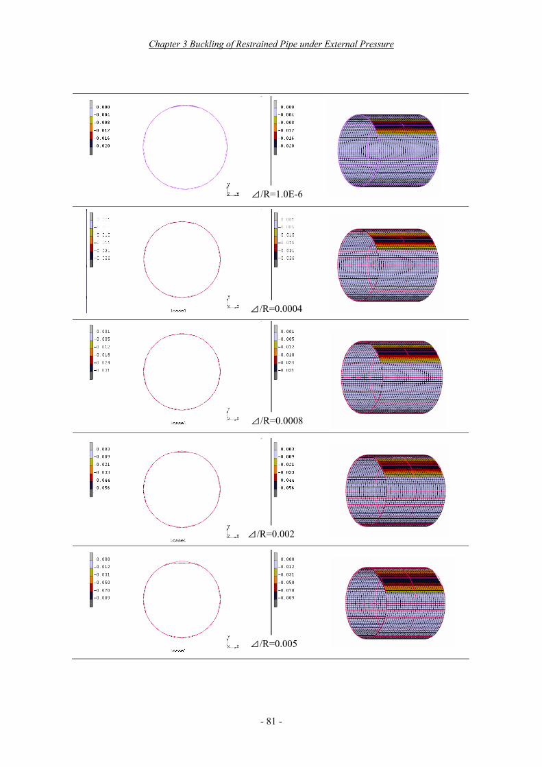
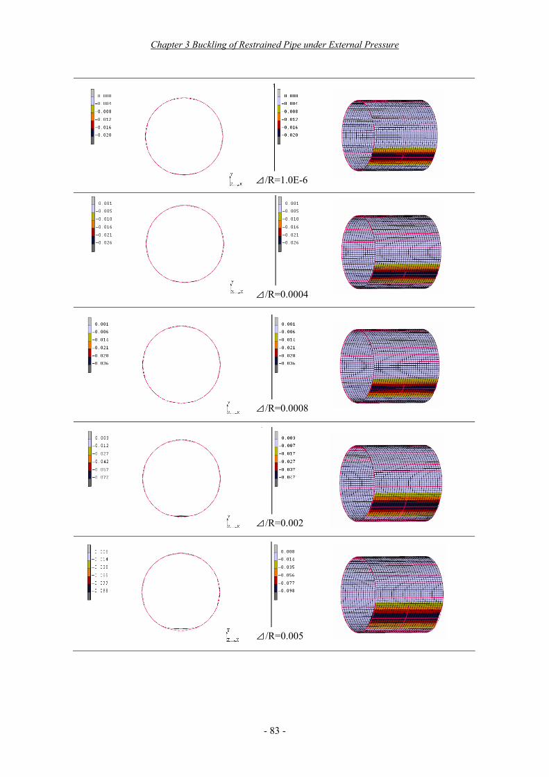
summarized. As the numerical analysis results, the behavior of external pressure and radial displacement of all models is focused as well as the failure mode in terms of radial displacement and VonMise stress. As for the displacement, the nodes located in single-lobe buckling area are used to provide the radial displacement relation. Where, all the numerical results of the model3 are presented as an example. The pressure-displacement curves with respect to the gap ratio of model3 are given for the two loading cases as shown in Fig. 3.11 a) and b), and the corresponding failure modes are summarized in Fig. 3.12 a) and b), respectively, in terms of radial deformation.
Chapter 3 Buckling of Restrained Pipe under External Pressure
- 80 -
0
500
1000
1500
2000
2500
-0.3-0.25-0.2-0.15-0.1-0.050
Radial displacement (m)
Exte
rnal
pre
ssur
e (kN
/m2 )
a) Loading case1 ( LC1)
0
500
1000
1500
2000
2500
-0.3-0.25-0.2-0.15-0.1-0.050
Radial displacement (m)
Exte
rnal
pre
ssur
e (kN
/m2 )
b) Loading case2 ( LC2) Fig. 3.11 Pressure-displacement behavior with different gap ratio ( Model3 )
0.0004
Δ/R=1.0E-6
0.0008
0.002
0.005
0.01 0.015 0.02 0.0250.05
0.0004
Δ/R=1.0E-6
0.0008
0.002
0.005
0.01 0.015 0.02 0.025 0.05
Chapter 3 Buckling of Restrained Pipe under External Pressure
- 81 -
⊿/R=0.0004
⊿/R=1.0E-6
⊿/R=0.0008
⊿/R=0.002
⊿/R=0.005

Chapter 3 Buckling of Restrained Pipe under External Pressure
- 82 -
1
Fig. 3.12 a) Radial deformation of failure mode under LC1 (Model3)
⊿/R=0.01
⊿/R=0.015
⊿/R=0.02
⊿/R=0.025
⊿/R=0.05
Chapter 3 Buckling of Restrained Pipe under External Pressure
- 83 -
1
⊿/R=1.0E-6
⊿/R=0.0004
⊿/R=0.0008
⊿/R=0.002
⊿/R=0.005
Chapter 3 Buckling of Restrained Pipe under External Pressure
- 84 -
1
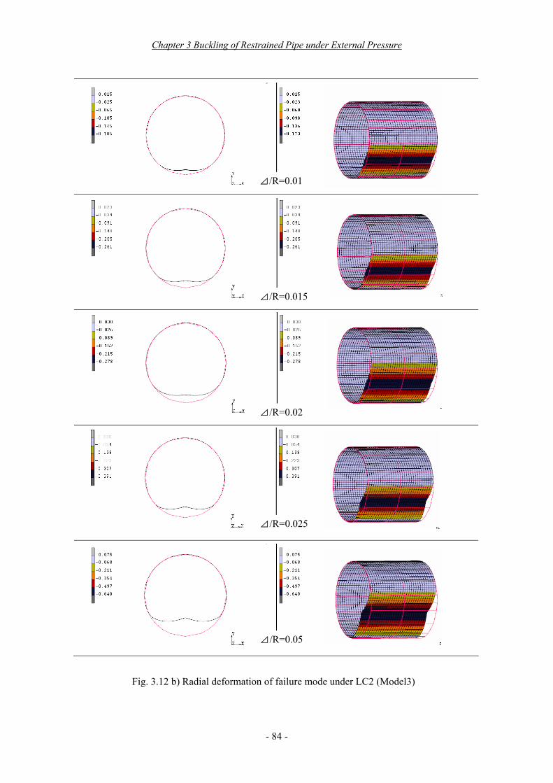
Fig. 3.12 b) Radial deformation of failure mode under LC2 (Model3)
⊿/R=0.01
⊿/R=0.015
⊿/R=0.02
⊿/R=0.025
⊿/R=0.05

Chapter 3 Buckling of Restrained Pipe under External Pressure
- 85 -
From the Fig. 3.11 a) and b), the encased plain pipe failed in single-lobe buckling and the critical pressure increases with the initial gap declining. In addition, it can be easily recognized that the single-lobe buckling occurred at crown and the corresponding failure inward deformation becomes large with the initial gap increasing for LC1 from Fig. 3.11 a) and b). On the contrary, the single-lobe buckling occurred at invert and its inward failure deformation increases with the increase of initial gap for LC2 of self-weigh and hydrostatic pressure. The similar results can be recognized from the Fig. 3.12 a) and b). As the deformation development, the crown of pipe detaches from host wall with the inward deformation increasing, while the other part deformed outward and attaches the host wall as the external pressure increase, and the inward deformed area enlarges with the initial gap increase at critical pressure.
Moreover, the consideration on predicting the buckling location is also verified, in which the single-lobe buckling of encased liner can be predicted according to the initial loading conditions, and always occur at the location with the larger gap under initial loads. Accordingly, it is valid to predict the buckling location through comparing the buoyancy and self weight based on the initial acting loads. Particularly, the buckle location of practical encased liner can be predicted validly by geometrical ratio of radius to thickness for plain liner, with respective to the practical loading conditions of self-weight and non-uniform hydrostatic pressure, considering the fact that single-lobe buckling of all models with R/t larger 15.6 occurred at invert. As the failure mechanism of encased liner, the Jacobsen’s consideration may be more reasonable and practical. When an encased pipe with initial annular gap is subjected to the external pressure loads, the deformations will vary from location around liner considering the external loads is not only a uniform pressure and the liner has initial shape imperfection. With external pressure increase, the outward deformation will be enlarged in one part of liner until outward deformation is restrained by host lining, while a single-lobe is formed in another part of liner with the inward deformation. The liner then fails when the inward deformed part liner comes to failure. The failure criterion is defined by Jacobsen as that the most outer fiber reaching the yield point. However, the failure criterion should be further discussed, although the formation of single-lobe and the failure mechanism is well explained.

Chapter 3 Buckling of Restrained Pipe under External Pressure
- 86 -
2) Discussion of critical pressure and existing buckling theories The critical pressure is obtained from the pressure-displacement behavior by only using the
peak value for LC1, while for LC2 the critical pressure should be adopted the total of peak value and the additional part of non-uniform pressure. However, the critical pressure in LC2 is difficult to estimate because the part of non-uniform pressure varies with the focused location. Where, the water pressures at bottom and center, representing the average pressure and maximum pressure, respectively are considered as the critical pressures of LC2. The relation of the critical pressure and gap ratio under two loading conditions obtained from numerical analysis are given for all the models as shown in Figs. 3.13-17, and the theoretical results calculated using equations of Amustutz and Jacobsen are also plotted on these figures. To explicitly show the relation of buckling pressure and gap ratio, the logarithmic type graphs are used.
Since the Glock’s equation is usually recommended for calculation of close-fitted pipe, the investigation of the critical pressure is carried out with respect to the gap case1, and the comparison results are listed in Table 3.4. Where, Pcr_G., Pcr_A. and Pcr_J. denote the theoretical critical pressure of Glock, Amustutz and Jacobsen, Pcr_num.1 are Pcr_num.2 represent the numerical values of LC1 and LC2, respectively. In addition, since the concept of comparing the buckling pressure for unsupported and encased liner has been employed by both researcher and developers of design codes, using an enhancement factor K, which is used to define the critical pressure for the encased liner, the enhancement factor K is computed and described in Figs. 3.18, with respect to the ratio of radius to thickness and gap to radius. Where, the enhancement factor is calculated by Eq. (3.7) using the numerical critical pressure of LC1 and LC2, respectively.
0
50100
150
200250
300
350
400450
500
0.0001 0.001 0.01 0.1Δ/R
Crit
ical
pre
ssur
e(kN
/m2 )
Numerical (Self-weight & uniform pressure)Numerical (Self-weight & water pressure)Theoretical (Amstuzu)Theoretical (Jacobsen)
Average water pressure Maximum water pressure Fig. 3.13 Comparison of theoretical and numerical results (Model1, R/t=200)
0
50100
150
200250
300
350
400450
500
0.0001 0.001 0.01 0.1Δ/R
Crit
ical
pre
ssur
e(kN
/m2 )
Numerical (Self-weight & uniform pressure)Numerical (Self-weight & water pressure)Theoretical (Amstuzu)Theoretical (Jacobsen)

Chapter 3 Buckling of Restrained Pipe under External Pressure
- 87 -
0
200
400
600
800
1000
1200
0.0001 0.001 0.01 0.1Δ/R
Crit
ical
pre
ssur
e(kN
/m2 )
Numerical (Self-weight & uniform pressure)Numerical (Self-weight & water pressure)Theoretical (Amstuzu)Theoretical (Jacobsen)
Average water pressure Maximum water pressure Fig. 3.14 Comparison of theoretical and numerical results (Model2, R/t=125)
0
500
1000
1500
2000
2500
3000
0.0001 0.001 0.01 0.1Δ/R
Crit
ical
pre
ssur
e(kN
/m2 )
Numerical (Self-weight & uniform pressure)Numerical (Self-weight & water pressure)Theoretical (Amstuzu)Theoretical (Jacobsen)
Average water pressure Maximum water pressure
Fig. 3.15 Comparison of theoretical and numerical results (Model3, R/t=75)
0
1000
2000
3000
4000
5000
0.0001 0.001 0.01 0.1Δ/R
Crit
ical
pre
ssur
e(kN
/m2 )
Numerical (Self-weight & uniform pressure)Numerical (Self-weight & water pressure)Theoretical (Amstuzu)Theoretical (Jacobsen)
Average water pressure Maximum water pressure Fig. 3.16 Comparison of theoretical and numerical results (Model4, R/t=50)
0
200
400
600
800
1000
1200
0.0001 0.001 0.01 0.1Δ/R
Crit
ical
pre
ssur
e(kN
/m2 )
Numerical (Self-weight & uniform pressure)Numerical (Self-weight & water pressure)Theoretical (Amstuzu)Theoretical (Jacobsen)
0
500
1000
1500
2000
2500
3000
0.0001 0.001 0.01 0.1Δ/R
Crit
ical
pre
ssur
e(kN
/m2 )
Numerical (Self-weight & uniform pressure)Numerical (Self-weight & water pressure)Theoretical (Amstuzu)Theoretical (Jacobsen)
0
1000
2000
3000
4000
5000
0.0001 0.001 0.01 0.1Δ/R
Crit
ical
pre
ssur
e(kN
/m2 )
Numerical (Self-weight & uniform pressure)Numerical (Self-weight & water pressure)Theoretical (Amstuzu)Theoretical (Jacobsen)
Chapter 3 Buckling of Restrained Pipe under External Pressure
- 88 -
0100020003000400050006000700080009000
10000
0.0001 0.001 0.01 0.1Δ/R
Crit
ical
pre
ssur
e(kN
/m2 )
Numerical (Self-weight & uniform pressure)Numerical (Self-weight & water pressure)Theoretical (Amstuzu)Theoretical (Jacobsen)
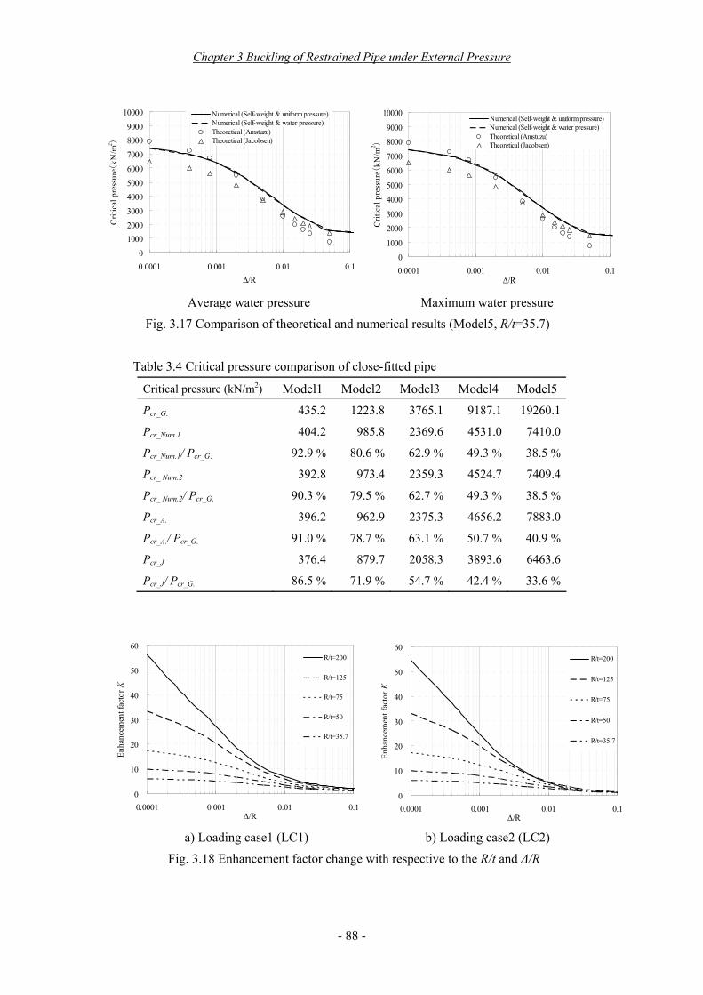
Average water pressure Maximum water pressure Fig. 3.17 Comparison of theoretical and numerical results (Model5, R/t=35.7)
Table 3.4 Critical pressure comparison of close-fitted pipe
Critical pressure (kN/m2) Model1 Model2 Model3 Model4 Model5 Pcr_G. 435.2 1223.8 3765.1 9187.1 19260.1
Pcr_Num.1 404.2 985.8 2369.6 4531.0 7410.0
Pcr_Num.1/ Pcr_G. 92.9 % 80.6 % 62.9 % 49.3 % 38.5 %
Pcr_ Num.2 392.8 973.4 2359.3 4524.7 7409.4
Pcr_ Num.2/ Pcr_G. 90.3 % 79.5 % 62.7 % 49.3 % 38.5 %
Pcr_A. 396.2 962.9 2375.3 4656.2 7883.0
Pcr_A./ Pcr_G. 91.0 % 78.7 % 63.1 % 50.7 % 40.9 %
Pcr_J 376.4 879.7 2058.3 3893.6 6463.6
Pcr_J/ Pcr_G. 86.5 % 71.9 % 54.7 % 42.4 % 33.6 %
0
10
20
30
40
50
60
0.0001 0.001 0.01 0.1Δ/R
Enha
ncem
ent f
acto
r K
R/t=200
R/t=125
R/t=75
R/t=50
R/t=35.7
a) Loading case1 (LC1) b) Loading case2 (LC2)
Fig. 3.18 Enhancement factor change with respective to the R/t and Δ/R
01000
20003000
40005000
60007000
80009000
10000
0.0001 0.001 0.01 0.1Δ/R
Crit
ical
pre
ssur
e(kN
/m2 )
Numerical (Self-weight & uniform pressure)Numerical (Self-weight & water pressure)Theoretical (Amstuzu)Theoretical (Jacobsen)
0
10
20
30
40
50
60
0.0001 0.001 0.01 0.1Δ/R
Enha
ncem
ent f
acto
r K
R/t=200
R/t=125
R/t=75
R/t=50
R/t=35.7
Chapter 3 Buckling of Restrained Pipe under External Pressure
- 89 -
From the above Figs. 3.13-17, it can be found that the critical pressure increases with the decreasing of gap ratio and the increasing of thickness. For all models with different thickness, the numerical results of buckling pressure under LC1 of self-weight and uniform external pressure agree well with that under LC2 of self-weight and hydrostatic pressure in general for any gap. Particularly, the critical pressures of two loading cases are almost identical to each other when the critical pressure of LC2 employs the maximum water pressure. Considering the bucking under LC2 of all the models occurred at invert, this may also indicate the critical pressure should apply the hydrostatic pressure of buckled location. Moreover, as single lobe buckling, the material failure of inward deformed part of liner cause the failure of general encased liner can be found, which has been discussed above.
As for the theoretical equations, generally the Amstutz’s equations give reasonable results which are agreement with the numerical results except model4 and model5 with radius to thickness ratio less than 50; while Jacobsen’s equations provide conservational results, especially for cases with smaller gap ratio. Moreover, for Amstutz’s buckling equations, the trend that the less the radius to thickness ratio is, the more the analytical critical pressure is agreeable with the numerical results can also be found. Whereas for Jacobsen’s buckling equations, the trend that the greater the gap to radius ratio is, the more the agreement between theoretical and numerical results can be obtained.
However, since Amstutz’s buckling equations can only be applied when the variation ε satisfies the requirement of in ranges 5 to20, and the corresponding judgment method in buckling pressure has been discussed, the method can be used to judge the results, as well as their verifications. From the Table 3.3 and the Figs. 3.13-17, that the judgment method using critical pressure is rather valid can be understood. The difference between theoretical and numerical pressure becomes greater when the critical pressure is less than the lower limits: 53 kN/m2 for model1, 215 kN/m2 for model2, 996 kN/m2 for model3, 3360 kN/m2 for model4 and 9220 kN/m2 for model5, respectively. Furthermore, that the thicker the pipe is, the more difficult the Amstutz’s equations can be applied is also confirmed, especially the model5 are completely out of the application range.
On the other hand, that the thicker the liner is the more conservational the Jacobsen’s theoretical critical pressure can also be concluded. The failure criterion of the most outer fiber yielding can be considered as the cause. For a thin wall liner the yielding of the most outer fiber at the point with maximum inward deformation can cause pipe failure; while for a thick wall pipe the liner is difficult to fail when the most outer fiber reaches the yield point because the cross section of inward deformed liner is rather high and is mainly subjected to bending force during failure process of single-lobe buckling. The consistent agreement between theoretical and numerical critical pressure of model1 with ratio of radius to thickness 200 as shown in Fig. 3.13 could be the good evidence. In addition, Jacobsen’s equations can provide
Chapter 3 Buckling of Restrained Pipe under External Pressure
- 90 -
a safe design for all cases of gap ratio less than 0.01, while for case with larger gap the application of Jacobsen’s equations should be carefully cautious, especially the critical pressure is possible to be over-estimated for a thinner liner.
Since the critical pressures are almost identical even the liners have different initial states of shape and stresses produced by different initial loading conditions, the initial imperfections of shape and stress distribution have little effects on single-lobe buckling of encased liner may be considered. This can be explained from the mechanism of single-lobe buckling, the imperfections will be adjusted during the single-lobe formation. In addition, the liner failure is just determined by material failure of inward deformed liner wall and the critical pressure is almost decided by the bending capacity of the inward deformed part. Moreover, that the effects of self weight and non-uniform pressure on single-lobe buckling are very limited can also be considered. The self-weight and non-uniform water pressure only affect the buckling location from crown to invert when the buoyancy is larger than the self-weight of liner.
Otherwise, as the Glock’s equation usually applied for the tightly fitted liner, the dangerous critical pressure is always given can be found from the critical pressure comparing with the analytical and numerical results as shown in Table 3.4. And, the more dangerous critical pressure is given by Glock’s equation with the increasing of ratio of radius to thickness. Since the critical pressure is related with not only the ratio of radius to thickness but also the yielding stress, elastic modulus, and the gap ratio in numerical analysis and Amstutz’s or Jacobsen’s buckling equations, while only the ratio of radius to thickness in Glock’s bucking equation, the Glock’s equation is not able to recommend, especially for the tunnel liner installed in separated water tunnel structure. As the enhancement factor widely adopted in design codes, the enhancement factor decreases with the inclining of the radius to thickness ratio and gap ratio in general is indicated explicitly in Fig. 3.18, no matter for LC1 or LC2. Additionally, Aggarwall and Cooper indicated that the values of the enhancement factor varied from 6.5 to 25.8 with a range of pipe of radius to thickness ratio approximately from 30 to 90, and 46 of 49 tests gave a value of K greater than 7. While another tests done by Lo and Zhang gave the enhancement factors ranged from 9.66 to 15.1. In the current study, the enhancement factor of tightly fitted case is 17, 10 and 6 for mode3, model4 and model5 with radius to thickness ratio 75, 50 and 35.7, respectively. This may also identify the numerical analysis rather sound. However, for the steel liner in the current study, the concept of enhancement may be meaningless since it is considered as loosely fitted liner and the enhance factor varies with not only the radius to thickness ratio but also the gap ratio.
Chapter 3 Buckling of Restrained Pipe under External Pressure
- 91 -
Summary In general, the mechanism of the single-lobe buckling can be explained that the encased liner
experiences the formulation of detached part and attached part of liner, and the single-lobe formulation in attached liner in two stages under the external pressure, then the finally material failure causes the liner failure. As the buckling location, the presented prediction method can be used to estimate the buckling site accurately. The critical pressure increases with the decreasing of gap ratio and the increasing of thickness was indicted. The initial imperfections of shape and stress distribution have little effects on single-lobe buckling of encased liner was found. As the theoretical solution, the Amstutz’s equations can be used to accurately estimate critical pressure if the 5<ε <20 was satisfied, and the presented judgment method was tested the useful solution to judge variation ε using the critical pressure. On the other hand, Jacobsen’s equations always give a conservational critical pressure, then is recommended to design considering the complex conditions unpredicted in engineering. However, the Glock’s equation and concept of enhancement applied for the tightly fitted liner should not be used because the variable gaps must be taken into account in the current study.

Chapter 3 Buckling of Restrained Pipe under External Pressure
- 92 -
3.4.3 Buckling of Stiffened Liner Numerical Analysis and Results
1) Models and gap cases The numerical analysis of buckling of stiffened pipes is carried out using the FE contact
analysis method. To investigate the effects of geometries of pipe on buckling, three kinds of steel pipe with different thicknesses were used as the numerical analysis models. Meanwhile, as the effects of the stiffening conditions, three ring stiffeners with different cross sections, and three different stiffening spacing are employed in analysis. All the numerical analysis models are summarized in Table 3.5. However, since the initial gap is vital to restrained hydrostatic buckling, seven gap cases are considered in the current study, including the tightly fitted case and free case, as shown in Table 3.6. Otherwise, the modeling and material properties of stiffened liners can refer 3.4.1, where the modeling of encased liner and water tunnel lining was described as well as contact analysis. However, it should be noted the radius of the host lining is equal to the total of the mean radius of pipe, stiffener height and the gap.
Table 3.5 Analysis models (stiffened pipe)
Pipe geometrics Stiffener Radius R (m)
Wall thickness t (mm)
High hr (mm)
Thicknesstr (mm)
Spacing S (m)
1.5 5
10 20
35 10 20 30
0.5 1.0 1.5
Table 3.6 Gap cases (stiffened pipe)
Gap Gap ratio Host radiusCases
Δ (mm) Δ/R R' (m)
Case1 0 0.0 1.5350 Case2 0.6 0.0004 1.5356 Case3 0.9 0.0006 1.5359 Case4 1.5 0.001 1.5365 Case5 7.5 0.005 1.5425 Case6 45 0.03 1.5800 Case7 1500 1.0 3.0350

Chapter 3 Buckling of Restrained Pipe under External Pressure
- 93 -
2) Numerical analysis results As the numerical analysis results, the buckling mode was judged according to the buckling
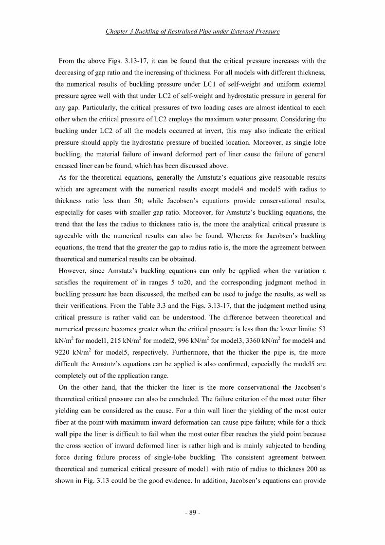
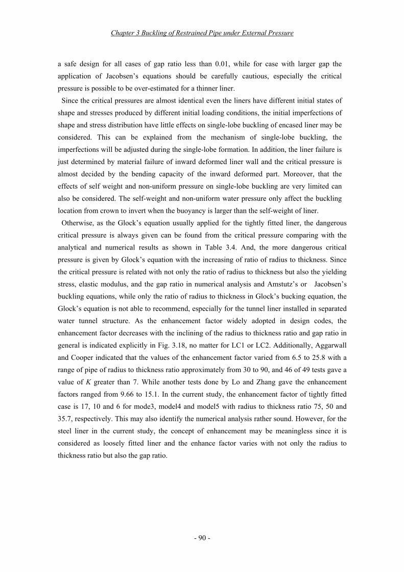
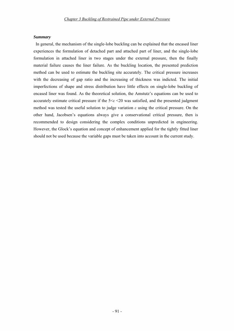
deformation, generally there are two kind bucking modes existing, inter-stiffener shell buckling and single-lobe buckling. Where, the examples of general buckling and local buckling are given in terms of the model with 5mm thickness and the stiffener with 30mm thickness and 1.5m spacing, as shown in Fig. 3.19. As the buckling pressure, the respective critical pressure was obtained using the same means of catching the peak pressure as applied in 3.4.2. The numerical analysis results of all models are shown in Fig. 3.20, Fig. 3.21 and Fig. 3.22, with respect to three kinds of stiffener spacing, in form of the behavior of critical pressure to gap ratio. Where the thickness of stiffer (tr) in the legends of the figures is used to represent the stiffness of stiffer, considering the height of stiffer is a constant value.
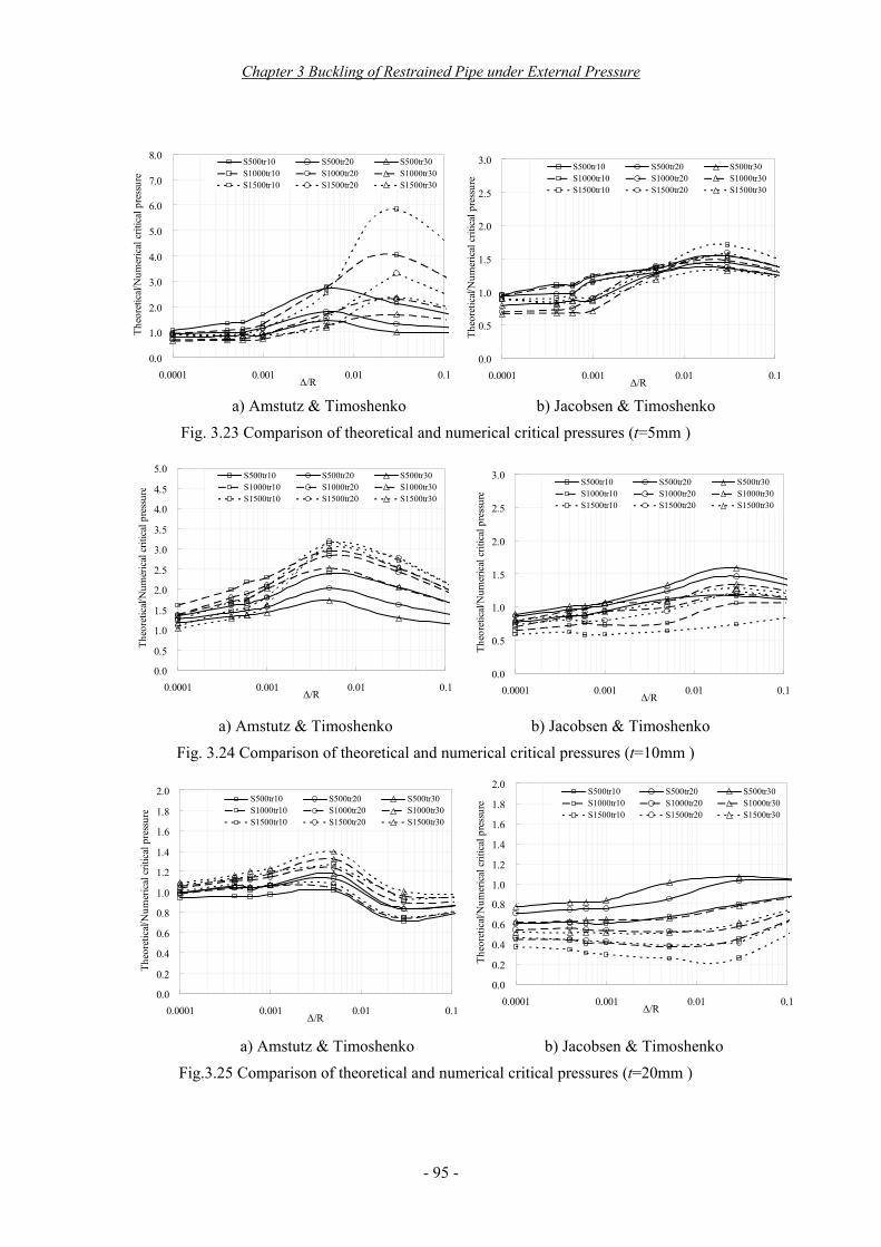
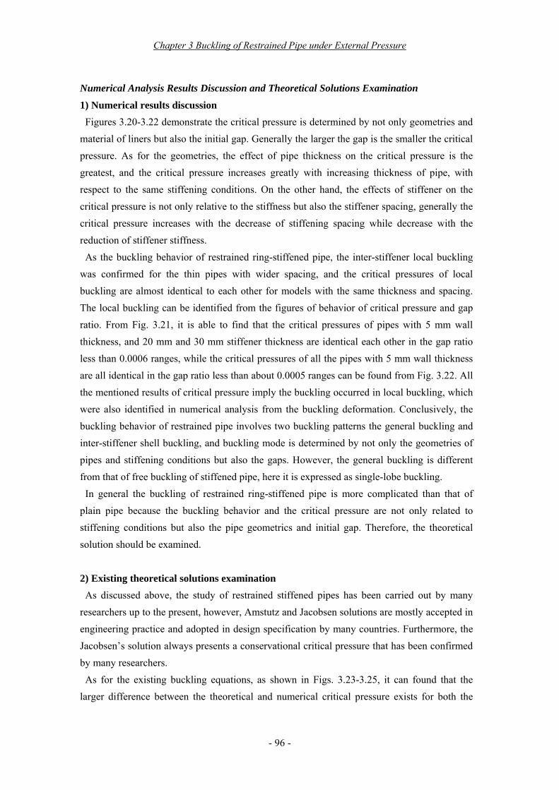
In addition, to investigate the two mentioned single-lobe buckling theories, the comparison of the numerical critical pressure with analytical results was also conducted, and the ratio of theoretical to numerical critical pressure was calculated. The comparing results with respect to the thickness of pipe are shown in Fig. 3.23, Fig. 3.24 and Fig. 3.25, respectively. Where the theoretical critical pressure was obtained based on the following solutions: Amstutz’s and Jacobsen’s equations are applied for single-lobe buckling, Timoshenko’s equation for local buckling.
a) Inter-stiffer shell buckling (Δ/R=0.001) b) Single-lobe buckling (Δ/R=0.005)
Fig. 3.19 Local and general buckling modes (t=5mm, tr=30mm, S=1.5m)
Chapter 3 Buckling of Restrained Pipe under External Pressure
- 94 -
0
500
1000
1500
2000
2500
3000
0.0001 0.001 0.01 0.1Δ/R
Crit
ical
pre
ssur
e (k
N/m
2 )
T5Tr10 T10Tr10 T20Tr10T5Tr20 T10Tr20 T20Tr20T5Tr30 T10Tr30 T20Tr30
Fig. 3.20 Behavior of critical pressure to gap ratio (S=0.5m )
0
500
1000
1500
2000
2500
0.0001 0.001 0.01 0.1Δ/R
Crit
ical
pre
ssur
e (k
N/m
2 )
T5Tr10 T10Tr10 T20Tr10T5Tr20 T10Tr20 T20Tr20T5Tr30 T10Tr30 T20Tr30
Fig. 3.21 Behavior of critical pressure to gap ratio (S=1.0m )
0
500
1000
1500
2000
2500
0.0001 0.001 0.01 0.1Δ/R
Crit
ical
pre
ssur
e (k
N/m
2 )
T5Tr10 T10Tr10 T20Tr10T5Tr20 T10Tr20 T20Tr20T5Tr30 T10Tr30 T20Tr30
Fig. 3.22 Behavior of critical pressure to gap ratio (S=1.5m )
Chapter 3 Buckling of Restrained Pipe under External Pressure
- 95 -
a) Amstutz & Timoshenko b) Jacobsen & Timoshenko
Fig. 3.23 Comparison of theoretical and numerical critical pressures (t=5mm )
a) Amstutz & Timoshenko b) Jacobsen & Timoshenko Fig. 3.24 Comparison of theoretical and numerical critical pressures (t=10mm )
a) Amstutz & Timoshenko b) Jacobsen & Timoshenko Fig.3.25 Comparison of theoretical and numerical critical pressures (t=20mm )
0.0
0.5
1.0
1.5
2.0
2.5
3.0
0.0001 0.001 0.01 0.1Δ/R
Theo
retic
al/N
umer
ical
crit
ical
pre
ssur
e
S500tr10 S500tr20 S500tr30S1000tr10 S1000tr20 S1000tr30S1500tr10 S1500tr20 S1500tr30
0.0
1.0
2.0
3.0
4.0
5.0
6.0
7.0
8.0
0.0001 0.001 0.01 0.1Δ/R
Theo
retic
al/N
umer
ical
crit
ical
pre
ssur
e
S500tr10 S500tr20 S500tr30S1000tr10 S1000tr20 S1000tr30S1500tr10 S1500tr20 S1500tr30
0.0
0.5
1.0
1.5
2.0
2.5
3.0
0.0001 0.001 0.01 0.1Δ/R
Theo
retic
al/N
umer
ical
crit
ical
pre
ssur
eS500tr10 S500tr20 S500tr30S1000tr10 S1000tr20 S1000tr30S1500tr10 S1500tr20 S1500tr30
0.0
0.2
0.4
0.6
0.8
1.0
1.2
1.4
1.6
1.8
2.0
0.0001 0.001 0.01 0.1Δ/R
Theo
retic
al/N
umer
ical
crit
ical
pre
ssur
e
S500tr10 S500tr20 S500tr30S1000tr10 S1000tr20 S1000tr30S1500tr10 S1500tr20 S1500tr30
0.0
0.2
0.4
0.6
0.8
1.0
1.2
1.4
1.6
1.8
2.0
0.0001 0.001 0.01 0.1Δ/R
Theo
retic
al/N
umer
ical
crit
ical
pre
ssur
e
S500tr10 S500tr20 S500tr30S1000tr10 S1000tr20 S1000tr30S1500tr10 S1500tr20 S1500tr30
0.0
0.5
1.0
1.5
2.0
2.5
3.0
3.5
4.0
4.5
5.0
0.0001 0.001 0.01 0.1Δ/R
Theo
retic
al/N
umer
ical
crit
ical
pre
ssur
e
S500tr10 S500tr20 S500tr30S1000tr10 S1000tr20 S1000tr30S1500tr10 S1500tr20 S1500tr30
Chapter 3 Buckling of Restrained Pipe under External Pressure
- 96 -
Numerical Analysis Results Discussion and Theoretical Solutions Examination
1) Numerical results discussion Figures 3.20-3.22 demonstrate the critical pressure is determined by not only geometries and
material of liners but also the initial gap. Generally the larger the gap is the smaller the critical pressure. As for the geometries, the effect of pipe thickness on the critical pressure is the greatest, and the critical pressure increases greatly with increasing thickness of pipe, with respect to the same stiffening conditions. On the other hand, the effects of stiffener on the critical pressure is not only relative to the stiffness but also the stiffener spacing, generally the critical pressure increases with the decrease of stiffening spacing while decrease with the reduction of stiffener stiffness.
As the buckling behavior of restrained ring-stiffened pipe, the inter-stiffener local buckling was confirmed for the thin pipes with wider spacing, and the critical pressures of local buckling are almost identical to each other for models with the same thickness and spacing. The local buckling can be identified from the figures of behavior of critical pressure and gap ratio. From Fig. 3.21, it is able to find that the critical pressures of pipes with 5 mm wall thickness, and 20 mm and 30 mm stiffener thickness are identical each other in the gap ratio less than 0.0006 ranges, while the critical pressures of all the pipes with 5 mm wall thickness are all identical in the gap ratio less than about 0.0005 ranges can be found from Fig. 3.22. All the mentioned results of critical pressure imply the buckling occurred in local buckling, which were also identified in numerical analysis from the buckling deformation. Conclusively, the buckling behavior of restrained pipe involves two buckling patterns the general buckling and inter-stiffener shell buckling, and buckling mode is determined by not only the geometries of pipes and stiffening conditions but also the gaps. However, the general buckling is different from that of free buckling of stiffened pipe, here it is expressed as single-lobe buckling.
In general the buckling of restrained ring-stiffened pipe is more complicated than that of plain pipe because the buckling behavior and the critical pressure are not only related to stiffening conditions but also the pipe geometrics and initial gap. Therefore, the theoretical solution should be examined.
2) Existing theoretical solutions examination As discussed above, the study of restrained stiffened pipes has been carried out by many
researchers up to the present, however, Amstutz and Jacobsen solutions are mostly accepted in engineering practice and adopted in design specification by many countries. Furthermore, the Jacobsen’s solution always presents a conservational critical pressure that has been confirmed by many researchers.
As for the existing buckling equations, as shown in Figs. 3.23-3.25, it can found that the larger difference between the theoretical and numerical critical pressure exists for both the
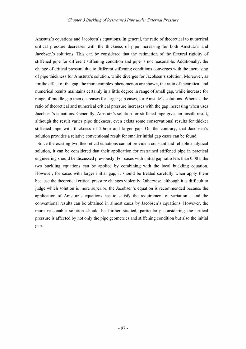
Chapter 3 Buckling of Restrained Pipe under External Pressure
- 97 -
Amstutz’s equations and Jacobsen’s equations. In general, the ratio of theoretical to numerical critical pressure decreases with the thickness of pipe increasing for both Amstutz’s and Jacobsen’s solutions. This can be considered that the estimation of the flexural rigidity of stiffened pipe for different stiffening condition and pipe is not reasonable. Additionally, the change of critical pressure due to different stiffening conditions converges with the increasing of pipe thickness for Amstutz’s solution, while diverges for Jacobsen’s solution. Moreover, as for the effect of the gap, the more complex phenomenon are shown, the ratio of theoretical and numerical results maintains certainly in a little degree in range of small gap, while increase for range of middle gap then decreases for larger gap cases, for Amstutz’s solutions. Whereas, the ratio of theoretical and numerical critical pressure increases with the gap increasing when uses Jacobsen’s equations. Generally, Amstutz’s solution for stiffened pipe gives an unsafe result, although the result varies pipe thickness, even exists some conservational results for thicker stiffened pipe with thickness of 20mm and larger gap. On the contrary, that Jacobsen’s solution provides a relative conventional result for smaller initial gap cases can be found.
Since the existing two theoretical equations cannot provide a constant and reliable analytical solution, it can be considered that their application for restrained stiffened pipe in practical engineering should be discussed previously. For cases with initial gap ratio less than 0.001, the two buckling equations can be applied by combining with the local buckling equation. However, for cases with larger initial gap, it should be treated carefully when apply them because the theoretical critical pressure changes violently. Otherwise, although it is difficult to judge which solution is more superior, the Jacobsen’s equation is recommended because the application of Amstutz’s equations has to satisfy the requirement of variation ε and the conventional results can be obtained in almost cases by Jacobsen’s equations. However, the more reasonable solution should be further studied, particularly considering the critical pressure is affected by not only the pipe geometries and stiffening condition but also the initial gap.

Chapter 3 Buckling of Restrained Pipe under External Pressure
- 98 -
3.5 Experimental Investigations of Single-lobe Buckling Failure
Amstutz’s and Jacobsen’s buckling equations are suitable to design thin plain liner in general, while they cannot solve the buckling problem of stiffened pipe was confirmed from the numerical discussions above. However since the steel liners are considered for practical utilization in terms of plain pipe and stiffened pipe, their failure should be investigated through experiment in details as well as the establishment of reliable solution. In the current study, the experimental approach is carried out to investigate failure of single-lobe buckling and to discuss the corresponding analytical solutions.
3.5.1 Experiment Design From the numerical analysis above, the single-lobe bucking is a procedure of single-lobe
formation and material failure has been confirmed for both plain liner and stiffened liner. An initial shape imperfection induced by the initial loading conditions causes the liner divided into detached part and attached part when subjected to external pressure afterward, while the initial gap determines the range of detached liner to form a single-lobe wave finally. The failure of liner due to single-lobe buckling is considered the failure of detached part of liner. Based on the part of the hypothesis, both Amstutz and Jacobsen derived their theoretical equations. However, the difference between their solutions is that the initial gap is used for determining the buckling range of liner in Jacobsen’s theory, whereas presenting a tensile stress necessary to close gap in Amstutz’s derivation. As the failure criterion, both Amstutz and Jacobsen adopted the stress in the extreme outer fiber of deformed plate reaches the yield point. Since the failure criterion is so vital while was only discussed for plain liner in both theoretical studies, whether it is rational, and similarly suitable for stiffened liner etc. should be investigated.
In the current study, the model experiment is carried out for plain pipe and stiffened pipe. As discussed above, considering the mechanism of a single-lobe formation is similar to the failure of single-lobe buckling of pipe under external pressure may be investigated by using an arch under center loading. The experiment therefore can be designed based on the assumption that the single-lobe buckling failure is the failure of the inward deflected plate. The design schematic of model experiment is shown in Fig. 3.26, where the model experiment is considered the case in which the upper half pipe detaches from host lining wall. The detailed build up is as follows: first, the upper half of liner is taken out as an analytical model because the lower half of pipe attached to host wall will maintains its circular shape and just provide a simple support to upper half pipe during single-lobe buckling process; next, the free half-circular arch can be considered the experimental model since the upper half pipe does still detach from host lining wall at the beginning; finally two symmetric edge loads as acting
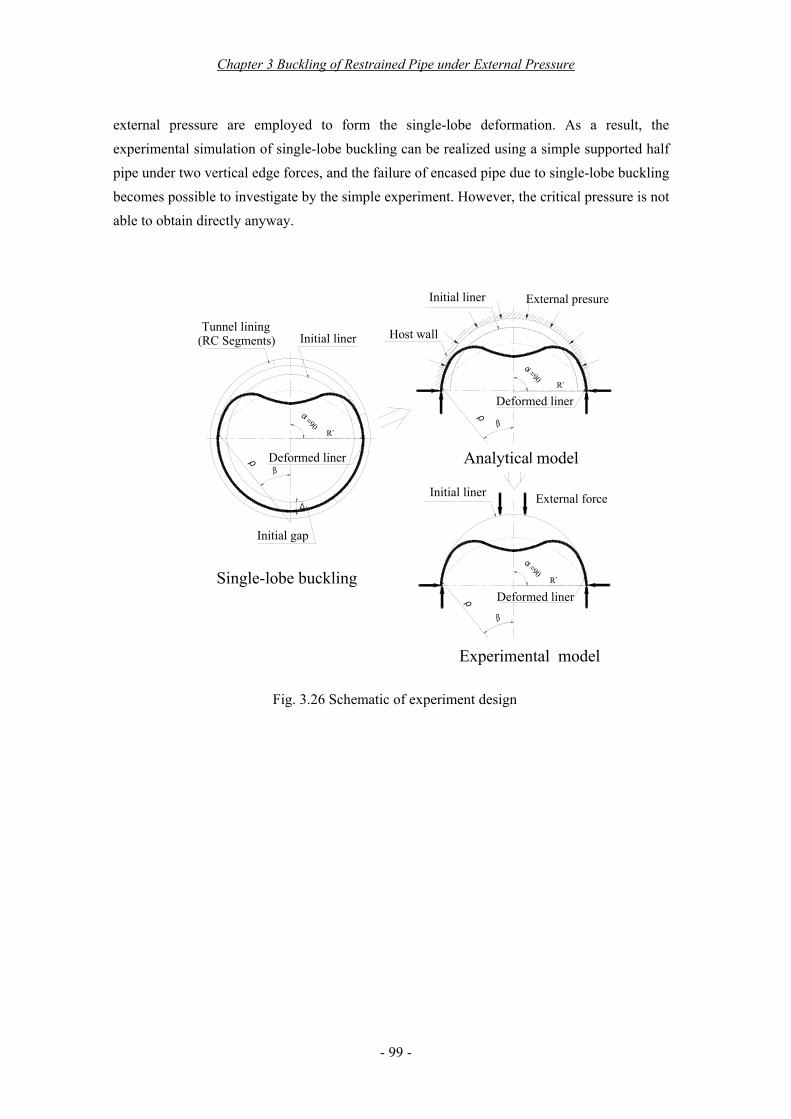
Chapter 3 Buckling of Restrained Pipe under External Pressure
- 99 -
external pressure are employed to form the single-lobe deformation. As a result, the experimental simulation of single-lobe buckling can be realized using a simple supported half pipe under two vertical edge forces, and the failure of encased pipe due to single-lobe buckling becomes possible to investigate by the simple experiment. However, the critical pressure is not able to obtain directly anyway.
External force
External presure
Experimental model
Analytical model
Δ
Deformed liner
Deformed liner
β
α
Initial gap
Tunnel lining(RC Segments)
=90
=90α
βR'
R'
Host wall
R'
=90α
β
Initial liner
Initial liner
Initial liner
Deformed liner
Single-lobe buckling
ρ
ρ
ρ
Fig. 3.26 Schematic of experiment design
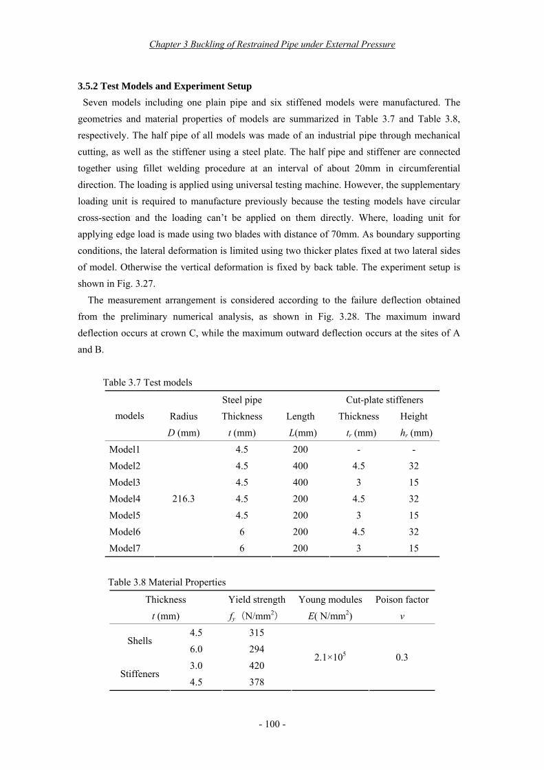
Chapter 3 Buckling of Restrained Pipe under External Pressure
- 100 -
3.5.2 Test Models and Experiment Setup Seven models including one plain pipe and six stiffened models were manufactured. The
geometries and material properties of models are summarized in Table 3.7 and Table 3.8, respectively. The half pipe of all models was made of an industrial pipe through mechanical cutting, as well as the stiffener using a steel plate. The half pipe and stiffener are connected together using fillet welding procedure at an interval of about 20mm in circumferential direction. The loading is applied using universal testing machine. However, the supplementary loading unit is required to manufacture previously because the testing models have circular cross-section and the loading can’t be applied on them directly. Where, loading unit for applying edge load is made using two blades with distance of 70mm. As boundary supporting conditions, the lateral deformation is limited using two thicker plates fixed at two lateral sides of model. Otherwise the vertical deformation is fixed by back table. The experiment setup is shown in Fig. 3.27.
The measurement arrangement is considered according to the failure deflection obtained from the preliminary numerical analysis, as shown in Fig. 3.28. The maximum inward deflection occurs at crown C, while the maximum outward deflection occurs at the sites of A and B.
Table 3.7 Test models
Steel pipe Cut-plate stiffeners models Radius
D (mm) Thickness
t (mm) Length L(mm)
Thickness tr (mm)
Height hr (mm)
Model1 4.5 200 - - Model2 4.5 400 4.5 32 Model3 4.5 400 3 15 Model4 4.5 200 4.5 32 Model5 4.5 200 3 15 Model6 6 200 4.5 32 Model7
216.3
6 200 3 15
Table 3.8 Material Properties
Yield strength Young modules Poison factor Thickness t (mm) fy(N/mm2) E( N/mm2) v
4.5 315 Shells
6.0 294 3.0 420
Stiffeners 4.5 378
2.1×10⁵ 0.3
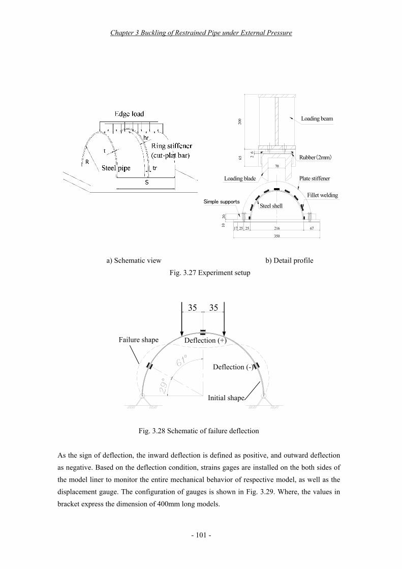
Chapter 3 Buckling of Restrained Pipe under External Pressure
- 101 -
a) Schematic view b) Detail profile
Fig. 3.27 Experiment setup
Fig. 3.28 Schematic of failure deflection
As the sign of deflection, the inward deflection is defined as positive, and outward deflection as negative. Based on the deflection condition, strains gages are installed on the both sides of the model liner to monitor the entire mechanical behavior of respective model, as well as the displacement gauge. The configuration of gauges is shown in Fig. 3.29. Where, the values in bracket express the dimension of 400mm long models.
Steel shell
Plate stiffenerLoading blade
26
Rubber(2mm)65
70
200
1020
252517 216 67
350
Fillet weldingSimple supports
Loading beam
3535
Deflection (+)
Deflection (-)
Failure shape
Initial shape

Chapter 3 Buckling of Restrained Pipe under External Pressure
- 102 -
a) General illustration and notions
b) Detailed configuration of strain gauges
Fig. 3.29 Measurement arrangement
Loading site
strain gauge(external and internal ) DisplacementGauge(D)
Gauge symbolC:CircumferentialL:LongitudinalI: InternalO:External
External side Internal side
Un-stiffened model
Loading site
Loading site
Stiffened model
External side Internal side
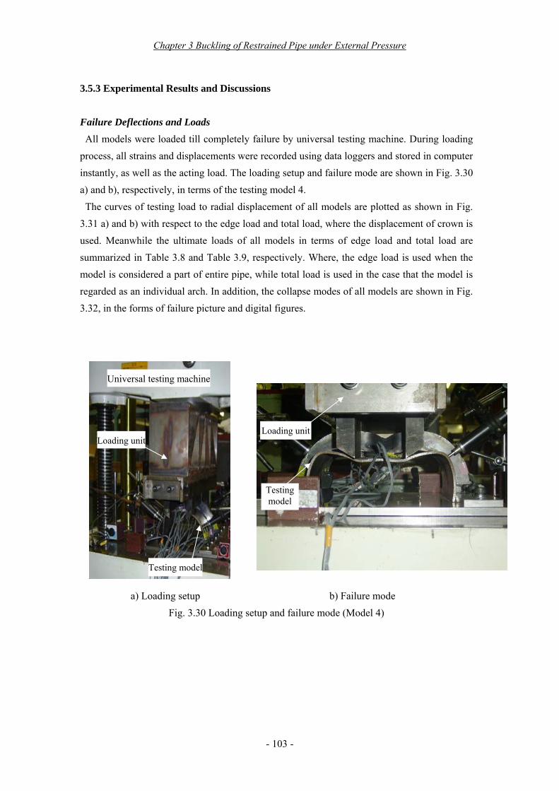
Chapter 3 Buckling of Restrained Pipe under External Pressure
- 103 -
3.5.3 Experimental Results and Discussions Failure Deflections and Loads
All models were loaded till completely failure by universal testing machine. During loading process, all strains and displacements were recorded using data loggers and stored in computer instantly, as well as the acting load. The loading setup and failure mode are shown in Fig. 3.30 a) and b), respectively, in terms of the testing model 4.
The curves of testing load to radial displacement of all models are plotted as shown in Fig. 3.31 a) and b) with respect to the edge load and total load, where the displacement of crown is used. Meanwhile the ultimate loads of all models in terms of edge load and total load are summarized in Table 3.8 and Table 3.9, respectively. Where, the edge load is used when the model is considered a part of entire pipe, while total load is used in the case that the model is regarded as an individual arch. In addition, the collapse modes of all models are shown in Fig. 3.32, in the forms of failure picture and digital figures.
a) Loading setup b) Failure mode Fig. 3.30 Loading setup and failure mode (Model 4)
Universal testing machine
Testing model
Loading unit
Testing model
Loading unit

Chapter 3 Buckling of Restrained Pipe under External Pressure
- 104 -
0
50
100
150
200
250
300
350
400
0 1 2 3 4 5 6 7 8 9 10 11 12 13 14 15Radial displacement of crown δ (mm)
Testi
ng lo
ad P
(kN
/m )
Model1Model2Model3Model4Model5Model6Model7
a) In edge load
0
20
40
60
80
100
120
140
160
180
0 1 2 3 4 5 6 7 8 9 10 11 12 13 14 15Radial displacement of crown δ (mm)
Testi
ng lo
ad F
(kN )
Model1Model2Model3Model4Model5Model6Model7
b) In total load Fig. 3.31 Testing load versus radial displacement at crown
Table 3.9 a) Collapse load of model as a part of pipe (in edge load)
Model Model1 Model2 Model3 Model4 Model5 Model6 Model7 Collapse load P (kN/m) 101.5 197.3 129.3 287.3 162.0 377.0 223.8
P/P1 (%) 100 194 127 283 160 371 220
Table 3.9 b) Collapse load of model as an individual arch (in total load)
Model Model1 Model2 Model3 Model4 Model5 Model6 Model7 Collapse
load F(kN) 40.6 157.8 103.4 114.9 64.8 150.8 89.5
F/F1 (%) 100 389 255 283 160 371 220
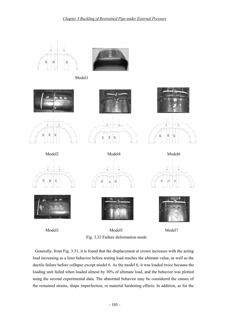
Chapter 3 Buckling of Restrained Pipe under External Pressure
- 105 -
Model1
Model2 Model4 Model6
Model3 Model5 Model7 Fig. 3.32 Failure deformation mode
Generally, from Fig. 3.31, it is found that the displacement at crown increases with the acting load increasing as a liner behavior before testing load reaches the ultimate value, as well as the ductile failure before collapse except model 6. As the model 6, it was loaded twice because the loading unit failed when loaded almost by 30% of ultimate load, and the behavior was plotted using the second experimental data. The abnormal behavior may be considered the causes of the remained strains, shape imperfection, or material hardening effects. In addition, as for the
85 8589
63 66 65
93 97 9585 8385
75 73 7570 67 7083 80 81

Chapter 3 Buckling of Restrained Pipe under External Pressure
- 106 -
thin wall pipe, the model2 and model4 stiffened with higher stiffener fail when the crown downwards about 10 mm, accompanying with the displacement increasing, testing load decreasing sharply. While the model1, model3 and model5 stiffened with smaller stiffener, the ductile behavior maintains in a large range of displacement without testing load decreasing extremely. However, as the model6 and model7, the collapse comes soon after reaching the ultimate load. Moreover, as shown in Fig. 3.32, the failure of all stiffened models were accompanied with striping of stiffener, and out-plane deformation of two waves for smaller stiffener, one wave for larger stiffener are formed at crown of stiffener.
As the loading resistance capacity in edge load, that the thicker of pipe is, the more great the ultimate load is, whereas the loading resistance capacity decrease with the stiffener spacing increase can be found from Fig. 3.31 a) and Table 3.9 a). Also the great influence of stiffener’s size on loading resistance capacity is illustrated, the larger the stiffener the higher the loading resistance capacity. All the results are same with the numerical results on the buckling of encased liner discussed above. Accordingly, this can prove the validation of the current experiment for investigation of the single-lobe buckling failure.
On the other hand, from the total load, the interacting range of stiffener and pipe can be investigated in certain extent. Form the Fig. 3.31 b) or Table 3.9 b), the ultimate load of 400mm long model2 is about the sum of length 200mm model4 with same stiffener and length 200mm un-stiffened model1 can be found. The same relation also exists for model3 and model5. This may verify the existence of effective width of stiffener because the influence of stiffener on pipe limits in a certain range.
Stains Distribution and Behavior Since the goal of this study is to investigate the failure criterion of pipe in single-lobe
deformation, the critical circumferential strains distributed at mostly deformed site should be confirmed in details, where the circumferential strains are given as shown in Figs. 3.33-3.39, in terms of external and internal strains located at mostly deformed locations, respectively. Meanwhile, the behaviors of circumferential strain to testing load of all models are summarized in Figs. 3.40-3.46, where the average value of most deformed locations along pipe was used and, the notions of CO, CI, + , - can refer the figure shown above, P and R denote the pipe and ring-stiffener respectively.
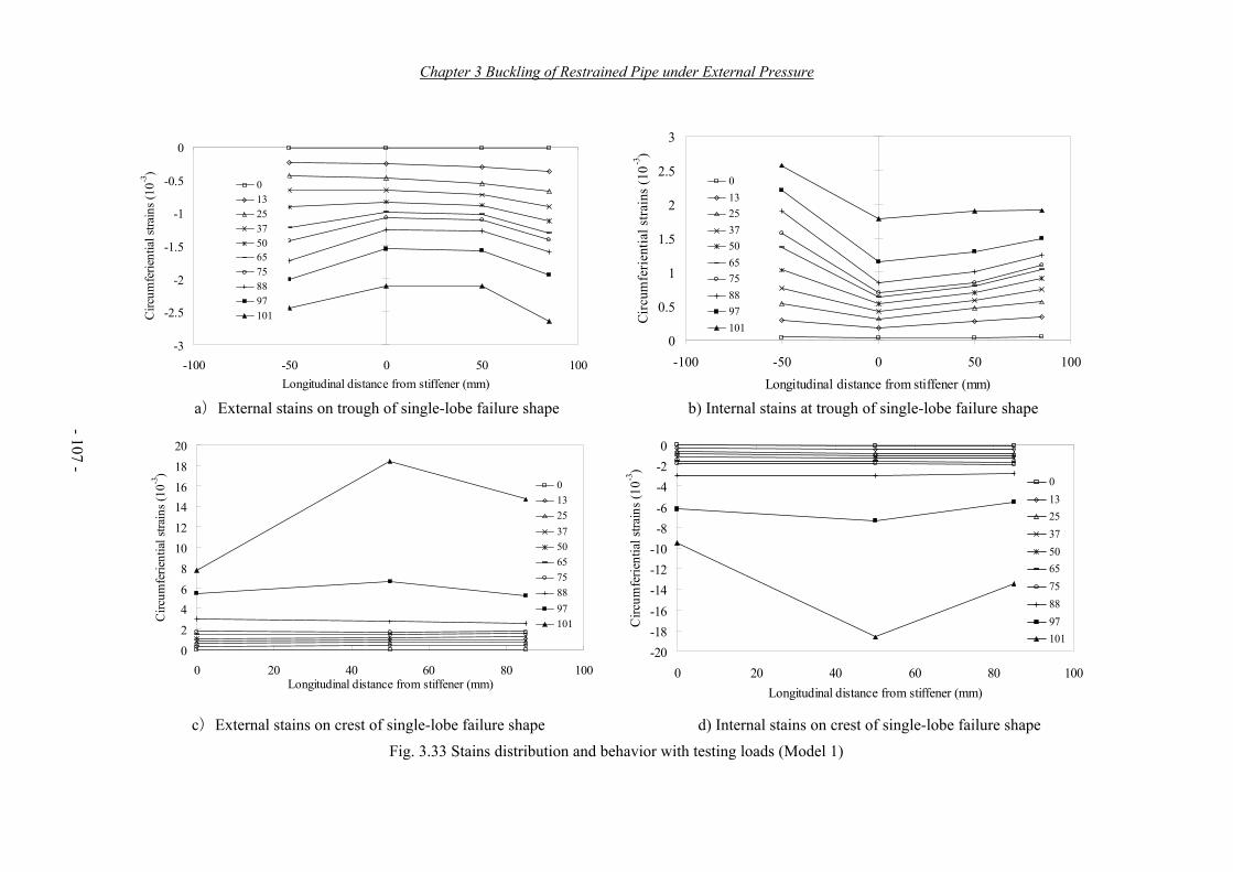
Chapter 3 Buckling of Restrained Pipe under External Pressure
- 107 -
a)External stains on trough of single-lobe failure shape b) Internal stains at trough of single-lobe failure shape
c)External stains on crest of single-lobe failure shape d) Internal stains on crest of single-lobe failure shape Fig. 3.33 Stains distribution and behavior with testing loads (Model 1)
0
0.5
1
1.5
2
2.5
3
-100 -50 0 50 100Longitudinal distance from stiffener (mm)
Circ
umfe
rient
ial s
train
s (10
-3)
013 25 37 50 65 75 88 97 101
-20-18-16-14-12-10-8-6-4-20
0 20 40 60 80 100Longitudinal distance from stiffener (mm)
Circ
umfe
rient
ial s
train
s (10
-3)
013 25 37 50 65 75 88 97 101
-3
-2.5
-2
-1.5
-1
-0.5
0
-100 -50 0 50 100Longitudinal distance from stiffener (mm)
Circ
umfe
rient
ial s
train
s (10
-3)
013 25 37 50 65 75 88 97 101
02468
101214161820
0 20 40 60 80 100Longitudinal distance from stiffener (mm)
Circ
umfe
rient
ial s
train
s (10
-3)
013 25 37 50 65 75 88 97 101

Chapter 3 Buckling of Restrained Pipe under External Pressure
- 108 -
a)External stains on trough of single-lobe failure shape b) Internal stains on trough of single-lobe failure shape
c)External stains on crest of single-lobe failure shape d) Internal stains on crest of single-lobe failure shape Fig. 3.34 Stains distribution and behavior with testing loads (Model2)
-2
0
2
4
6
8
10
0 50 100 150 200Longitudinal distance from stiffener (mm)
Circ
umfe
rient
ial s
train
s (10
-3)
0 12 38 62 87 99 114 125 138 149 162 176 187 196
-25
-20
-15
-10
-5
0
5
-100 -50 0 50 100 150 200Longitudinal distance from stiffener (mm)
Circ
umfe
rient
ial s
train
s (10
-3)
0 12 38 62 87 99 114 125 138 149 162 176 187 196
-1.5
-1
-0.5
0
0.5
1
1.5
2
-100 -50 0 50 100 150 200Longitudinal distance from stiffener (mm)
Circ
umfe
rient
ial s
train
s (10
-3) 0 12
38 62 87 99 114 125 138 149 162 176 187 196
-12
-10
-8
-6
-4
-2
0
0 50 100 150 200Longitudinal distance from stiffener (mm)
Circ
umfe
rient
ial s
train
s (10
-3)
0 12 38 62 87 99 114 125 138 149 162 176 187 196

Chapter 3 Buckling of Restrained Pipe under External Pressure
- 109 -
a)External stains on trough of single-lobe failure shape b) Internal stains on trough of single-lobe failure shape
c)External stains on crest of single-lobe failure shape d) Internal External stains on crest of single-lobe failure shape Fig. 3.35 Stains distribution and behavior with testing loads (Model3)
-35
-30
-25
-20
-15
-10
-5
0
-100 -50 0 50 100 150 200Longitudinal distance from stiffener (mm)
Circ
umfe
rient
ial s
train
s (10
-3)
0 1427 3237 5065 7491 101113 125129
0
10
20
30
40
50
60
0 50 100 150 200Longitudinal distance from stiffener (mm)
Circ
umfe
rient
ial s
train
s (10
-3)
0 1427 3237 5065 7491 101113 125129
0
0.5
1
1.5
2
2.5
3
3.5
4
-100 -50 0 50 100 150 200Longitudinal distance from stiffener (mm)
Circ
umfe
rient
ial s
train
s (10
-3)
0 1427 3237 5065 7491 101113 125129
-20-18-16-14-12-10-8-6-4-20
0 50 100 150 200Longitudinal distance from stiffener (mm)
Circ
umfe
rient
ial s
train
s (10
-3)
0 1427 3237 5065 7491 101113 125129

Chapter 3 Buckling of Restrained Pipe under External Pressure
- 110 -
a)External stains on trough of single-lobe failure shape b) Internal stains on trough of single-lobe failure shape
c)External stains on crest of single-lobe failure shape d) Internal stains on crest of single-lobe failure shape Fig. 3.36 Stains distribution and behavior with testing loads (Model4)
-25
-20
-15
-10
-5
0
5
-100 -50 0 50 100Longitudinal distance from stiffener (mm)
Circ
umfe
rient
ial s
train
s (10
-3)
0 31 51 83 102 127 154 182 201 225 253 276 285
-1-0.5
00.5
11.5
22.5
33.5
44.5
0 20 40 60 80 100Longitudinal distance from stiffener (mm)
Circ
umfe
rient
ial s
train
s (10
-3) 0 31 51 83 102 127 154
182 201 225 253 276 285
-3
-2
-1
0
1
2
3
4
-100 -50 0 50 100Longitudinal distance from stiffener (mm)
Circ
umfe
rient
ial s
train
s (10
-3)
0 31 51 83 102 127 154 182 201 225 253 276 285
-9
-8
-7
-6
-5
-4
-3
-2
-1
0
0 20 40 60 80 100Longitudinal distance from stiffener (mm)
Circ
umfe
rient
ial s
train
s (10
-3)
0 31 51 83 102 127 154 182 201 225 253 276 285
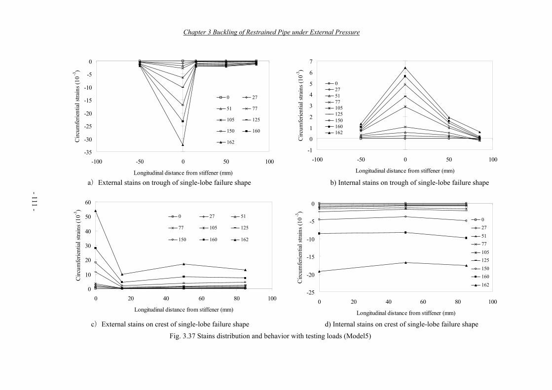
Chapter 3 Buckling of Restrained Pipe under External Pressure
- 111 -
a)External stains on trough of single-lobe failure shape b) Internal stains on trough of single-lobe failure shape
c)External stains on crest of single-lobe failure shape d) Internal stains on crest of single-lobe failure shape Fig. 3.37 Stains distribution and behavior with testing loads (Model5)
-35
-30
-25
-20
-15
-10
-5
0
-100 -50 0 50 100
Longitudinal distance from stiffener (mm)
Circ
umfe
rient
ial s
train
s (10
-3)
0 27
51 77
105 125
150 160
162
0
10
20
30
40
50
60
0 20 40 60 80 100
Longitudinal distance from stiffener (mm)
Circ
umfe
rient
ial s
train
s (10
-3)
0 27 51
77 105 125
150 160 162
-1
0
1
2
3
4
5
6
7
-100 -50 0 50 100
Longitudinal distance from stiffener (mm)
Circ
umfe
rient
ial s
train
s (10
-3)
0 27 51 77 105 125 150 160 162
-25
-20
-15
-10
-5
0
0 20 40 60 80 100
Longitudinal distance from stiffener (mm)
Circ
umfe
rient
ial s
train
s (10
-3)
0 27 51 77 105 125 150 160 162

Chapter 3 Buckling of Restrained Pipe under External Pressure
- 112 -
(a)External stains on trough of single-lobe failure shape (b) Internal stains on trough of single-lobe failure shape
c)External stains on crest of single-lobe failure shape d) Internal stains on crest of single-lobe failure shape Fig. 3.38 Stains distribution and behavior with testing loads (Model6)
-30
-25
-20
-15
-10
-5
0
5
-100 -50 0 50 100Longitudinal distance from stiffener (mm)
Circ
umfe
rient
ial s
train
s (10 -
3 )
0 51 96 124 154 175 202 231 254 299 330 363
-5
0
5
10
15
20
0 20 40 60 80 100Longitudinal distance from stiffener (mm)
Circ
umfe
rient
ial s
train
s (10
-3) 0 51 96 124
154 175 202 231
254 299 330 363
-2
-1.5
-1
-0.5
0
0.5
1
1.5
2
0 20 40 60 80 100Longitudinal distance from stiffener (mm)
Circ
umfe
rient
ial s
train
s (10
-3) 0 51 96 124 154 175
202 231 254 299 330 363
-8
-7
-6
-5
-4
-3
-2
-1
0
0 20 40 60 80 100Longitudinal distance from stiffener (mm)
Circ
umfe
rient
ial s
train
s (10
-3)
0 51 96 124 154 175
202 231 254 299 330 363
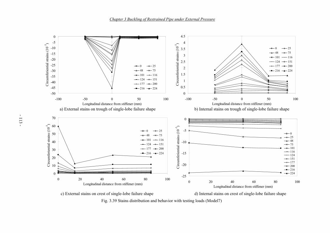
Chapter 3 Buckling of Restrained Pipe under External Pressure
- 113 -
a) External stains on trough of single-lobe failure shape b) Internal stains on trough of single-lobe failure shape
c) External stains on crest of single-lobe failure shape d) Internal stains on crest of single-lobe failure shape Fig. 3.39 Stains distribution and behavior with testing loads (Model7)
-50-45-40-35-30-25-20-15-10-50
-100 -50 0 50 100Longitudinal distance from stiffener (mm)
Circ
umfe
rient
ial s
train
s (10
-3)
0 25 48 75 101 116 124 151 177 200 216 224
0
10
20
30
40
50
60
70
0 20 40 60 80 100Longitudinal distance from stiffener (mm)
Circ
umfe
rient
ial s
train
s (10
-3)
0 25 48 75 101 116 124 151 177 200 216 224
0
0.5
1
1.5
2
2.5
3
3.5
4
4.5
-100 -50 0 50 100Longitudinal distance from stiffener (mm)
Circ
umfe
rient
ial s
train
s (10
-3)
0 25 48 75 101 116 124 151 177 200 216 224
-25
-20
-15
-10
-5
0
0 20 40 60 80 100Longitudinal distance from stiffener (mm)
Circ
umfe
rient
ial s
train
s (10
-3)
0 25 48 75 101 116 124 151 177 200 216 224
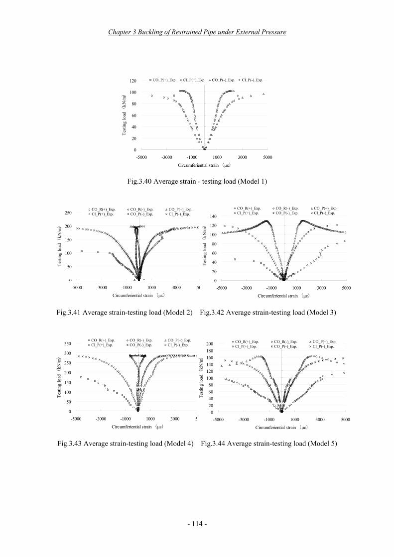
Chapter 3 Buckling of Restrained Pipe under External Pressure
- 114 -
0
20
40
60
80
100
120
-5000 -3000 -1000 1000 3000 5000
Circumferiential strain (με)
Testi
ng lo
ad (
kN/m)
CO_P(+)_Exp. CI_P(+)_Exp. CO_P(-)_Exp. CI_P(-)_Exp.
Fig.3.40 Average strain - testing load (Model 1)
0
50
100
150
200
250
-5000 -3000 -1000 1000 3000 5000
Circumferiential strain (με)
Testi
ng lo
ad (
kN/m)
CO_R(+)_Exp. CO_R(-)_Exp. CO_P(+)_Exp.CI_P(+)_Exp. CO_P(-)_Exp. CI_P(-)_Exp.
Fig.3.41 Average strain-testing load (Model 2) Fig.3.42 Average strain-testing load (Model 3)
0
50
100
150
200
250
300
350
-5000 -3000 -1000 1000 3000 5000
Circumferiential strain (με)
Testi
ng lo
ad (
kN/m)
CO_R(+)_Exp. CO_R(-)_Exp. CO_P(+)_Exp.CI_P(+)_Exp. CO_P(-)_Exp. CI_P(-)_Exp.
Fig.3.43 Average strain-testing load (Model 4) Fig.3.44 Average strain-testing load (Model 5)
0
20
40
60
80
100
120
140
-5000 -3000 -1000 1000 3000 5000
Circumferiential strain (με)
Testi
ng lo
ad (
kN/m)
CO_R(+)_Exp. CO_R(-)_Exp. CO_P(+)_Exp.CI_P(+)_Exp. CO_P(-)_Exp. CI_P(-)_Exp.
020406080
100120140160180200
-5000 -3000 -1000 1000 3000 5000
Circumferiential strain (με)
Testi
ng lo
ad (
kN/m)
CO_R(+)_Exp. CO_R(-)_Exp. CO_P(+)_Exp.CI_P(+)_Exp. CO_P(-)_Exp. CI_P(-)_Exp.

Chapter 3 Buckling of Restrained Pipe under External Pressure
- 115 -
050
100150200250300350400450
-5000 -3000 -1000 1000 3000 5000
Circumferiential strain (με)
Testi
ng lo
ad (
kN/m)
CO_R(+)_Exp. CO_R(-)_Exp. CO_P(+)_Exp.CI_P(+)_Exp. CO_P(-)_Exp. CI_P(-)_Exp.
Fig.3.45 Average strain- testing load (Model 6) Fig.3.46 Average strain-testing load (Model 7)
From Fig. 3.33 and Fig. 3.40, the failure behavior of plain pipe can be found, that the first yielding occurred at two sides with maximum outward deflection, however overall plain pipe failed after the maximum strain at crown beyond yielding point. It is indicated that the pipe with single-lobe deflection does not fail when the outer extreme fiber of maximum deflected location reaches yielding point, rather when three hinges are formed. Furthermore, the failure strains at crown reached 0.0025 at external side and 0.002 at internal side in average, although the yielding strain is 0.0015, and the yielded area has reached the 1/3 total cross section of pipe. Since the model1 with thickness 4.5mm, its ratio of radius to thickness is only 24, the yielding of outer fiber is not appreciate to be the failure criterion for thicker pipe can be considered. Accordingly, the critical pressure of single-lobe buckling failure cannot be accurately estimated if the pipe is too thick. The results discussed in 3.4.2 that the difference between numerical and theoretical critical pressure increase with thickness increasing may be explained well here.
On the other hand, the failure behaviors of stiffened pipe are more complicated can be found form these figures. Where the investigations are carried out in two cases: one for model with larger stiffener, another one for model with smaller stiffener, namely rigidly stiffened pipe and weakly stiffened pipe respectively.
For rigidly stiffened pipes of model2, model4 and model6, as shown in Figures 3.34, 3.36, 3.38, 3.41, 3.43 and 3.45, the strains in the most outer fiber of stiffener express a bending behavior of increasing with acting load, and agree well with the corresponding flexural deformations. While strains in the most outer fiber of pipe vary violently from the locations along pipe, even the abnormal stains appear at the locations near to stiffeners. The reason can be considered that the bending force is almost resisted by stiffeners because of its great flexural rigidity, whereas the pipe does not only resist the axial force but also the flexural deformation. The interacting effects of stiffener are rather great therefore can be found, as well as the failure criteria should not use the strain in the most outer fiber of stiffener, for rigidly stiffened pipe. However, the internal strains distributed at negative deflected location of pipe shows a stable
0
50
100
150
200
250
300
-5000 -3000 -1000 1000 3000 5000
Circumferiential strain (με)
Testi
ng lo
ad (
kN/m)
CO_R(+)_Exp. CO_R(-)_Exp. CO_P(+)_Exp.CI_P(+)_Exp. CO_P(-)_Exp. CI_P(-)_Exp.
Chapter 3 Buckling of Restrained Pipe under External Pressure
- 116 -
developing behavior with increasing of testing load along pipe, and the failure strains is about 6×10⁻³ for all three models. Considering the other stains developing behavior changes violently along pipe, the compressive strains located at the most outward deflected location of pipe may be appreciate to be used for the failure criterion of stiffened pipe with larger stiffener. Especially, since the largest inward and outward deformations are considered identical to each other in Jacobsen’s single-lobe buckling theory, the compressive strains in fibers with same distance from neutral axial should be identical for both locations. Therefore, it can be considered the rigidly stiffened pipe fails when the compressive strains in fiber at the same distance of internal surface to neutral axial reaches yielding point. Moreover, since the failure behavior is mainly determined by stiffener, the theoretical analysis can only consider the composed effective cross-section of stiffener and the co-operating strip of pipe. However, as the width of co-operating strip of pipe, named effective width (Be ), there are three kind definitions: 30t, 1.56(Rt)0.5 and 0.75S. And any computed value of the width of co-operating strip is rather arbitrary because the interaction between stiffener and pipe is rather complicated phenomenon which is not only related to the geometries of pipe and stiffener but also the internal forces. Thus, the effective width should be discussed and modified when it is used for single-lobe buckling theory.
On the other hand, for the weakly stiffened pipe of model3, model5 and model6, as shown in Figs. 3.35, 3.37, 3.39, 3.42, 3.44 and 3.46, all the behaviors of strain versus testing load, show the completed bending behavior similar to that of model1, and the strains distribution along pipe changes little. Moreover, the strains of external and internal surfaces express the compressive and tensile strain at crown, tensile and compressive strain at two sides, respectively, and increase with the testing loading. This may indicate that the interaction between stiffener and pipe is just limited for an adjacent strip and the mechanical behavior is controled by flexural rigidity of the overall stiffened pipe. Actually, all strains distributed on pipe maintain the same behavior and the closest distance of measured location to stiffener is only 15mm, about 3t. Therefore, the cross section including stiffener and the inter-stiffener shell should be used when discuss the single-lobe buckling. In addition, it is shown clearly that the failure of models occurs when the external compressive strains at pipe surface reaches yielding point. Accordingly, the failure criterion of weakly stiffened pipe can use the external strain located at crown of pipe.
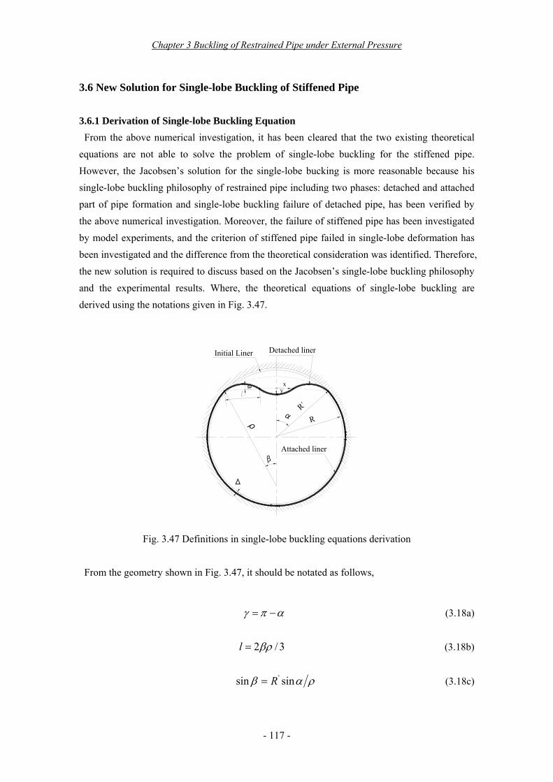
Chapter 3 Buckling of Restrained Pipe under External Pressure
- 117 -
3.6 New Solution for Single-lobe Buckling of Stiffened Pipe
3.6.1 Derivation of Single-lobe Buckling Equation From the above numerical investigation, it has been cleared that the two existing theoretical
equations are not able to solve the problem of single-lobe buckling for the stiffened pipe. However, the Jacobsen’s solution for the single-lobe bucking is more reasonable because his single-lobe buckling philosophy of restrained pipe including two phases: detached and attached part of pipe formation and single-lobe buckling failure of detached pipe, has been verified by the above numerical investigation. Moreover, the failure of stiffened pipe has been investigated by model experiments, and the criterion of stiffened pipe failed in single-lobe deformation has been investigated and the difference from the theoretical consideration was identified. Therefore, the new solution is required to discuss based on the Jacobsen’s single-lobe buckling philosophy and the experimental results. Where, the theoretical equations of single-lobe buckling are derived using the notations given in Fig. 3.47.
β
R'
α
Initial Liner
Attached liner
ρa x
y
R
Δ
Detached liner
Fig. 3.47 Definitions in single-lobe buckling equations derivation
From the geometry shown in Fig. 3.47, it should be notated as follows,
απγ −= (3.18a)
3/2βρ=l (3.18b)
ραβ sinsin 'R= (3.18c)

Chapter 3 Buckling of Restrained Pipe under External Pressure
- 118 -
βαρ sinsin'R= (3.18d)
βαβ sin3sin2 'Rl = (3.18e)
πβαα )tan( −= l (3.18f)
( ) ⎥⎦⎤⎢⎣⎡ +=
2
21 lallsπ (3.18g)
The circumference of the pipe before the external pressure starting to act is )(2 Δ−Rπ , and
the circumference of the pipe after sinusoidal wave has developed is slR 32 ' +γ , hence the
circumference has been reduced by slRR 32)(2 '' −−Δ− γπ . On the other hand, the reduction of the circumference may be written as an elastic deformation of the pipe circumference
tEp
tEpRR ρβργ 22
'' + .
The first equation is therefore,
tEp
tEpRRlRR S
ρβργγπ 2232)(2'
''' +=−−Δ− (3.19)
The second equation as the differential equation of the elastic deflected pipe, can be written as
EIMyxdyd −=+ 222 ρ . It is assumed that the elastic deflection line is of sinusoidal shape, therefore, lxay πcos= , lxlaxdyd ππ cos)( 2222 −= can be obtained. At the point x=0, )( 2222 laxdyd π−= may be introduced, and the second equation is obtained as follows,
3222 12 Etapala ρρπ −=+− (3.20)
The third equation is derived from the requirement that the stress in the most outer fiber of the plate reach the yield point. The component stresses are,
・Circumferential stress due to the external pressure ・Change of curvature from 1/R’ to 1/ρ ( flexural stretching) ・Bending stress due to the normal force and eccentricity.
The third equation can therefore be written as
2' 6)/1/1(2 tapRtEtpf y ρρρ +−+= (3.21)
Based on the three equations, Jacobsen derived the famous Jacobsen’s buckling equations for encased liner according to the assumed buckling deformed shape. Meanwhile the stiffened pipe has been discussed based on the assumptions: 1) the pipe shell between the rings can sustain the external pressure acting on ,as a free pipe held circular shape at two ends by the rings; and, 2) as
Chapter 3 Buckling of Restrained Pipe under External Pressure
- 119 -
the constants of cross-section of stiffened pipe, the moment of inertia I, cross-sectional area F and distance of focusing point from the neutral axis h are considered for the stiffener and the pipe shell with carrying width, the stiffener and the pipe shell between stiffeners and the distance of the outer fiber of stiffener, respectively. The buckling equations of restrained stiffened pipe is then shown as follows,
[ ] [ ][ ][ ]4)(tan1)sinsin(/)sinsin(12
)sinsin(1)49(12 2'3
222'
βαβαβπαβα
βαβαπβπ
−+−Δ−
+−−=
RFIR (3.22a)
( )33'
22
)sinsin(149βα
βπSR
IEPcr−
= (3.22b)
⎥⎦
⎤⎢⎣
⎡ −++⎟
⎠⎞
⎜⎝⎛ −=
βπβααβ
βα
αβ
sin3)tan(sin21
sinsin
sinsin1
''
' IFhR
EFSRP
Rh
Ef cry (3.22c)

Chapter 3 Buckling of Restrained Pipe under External Pressure
- 120 -
3.6.2 New Analytical Solution Jacobsen’s buckling equations although may give a sound result for restrained plain pipe,
however, the application for restrained stiffened pipe can not be recommended. The failure of stiffened pipe with single-lobe deformation is rather different from when the most outer fiber of stiffener reaches the yield point. It is therefore necessary to discuss the new solution. Herein, the analytical solution is discussed based on the experimental and the numerical analytical results.
Since the failure of restrained stiffened pipe varies from stiffening conditions, the solution should be started from the judgment of stiffening condition. From the experiment, the failure happened when the stress in the most outer fiber of pipe reaches yield point for weakly stiffened pipe, while when the most inner fiber yields for rigidly stiffened pipe. Otherwise, for rigidly stiffened pipe, the stiffeners and carrying strip of pipe can be considered the main system to resist external loads, whereas the overall stiffened pipe including the stiffener and the inter-stiffener shell should be considered the system to resist external loads for weakly stiffened pipe. In the following paragraphs, the analytical solution to solve the single-lobe buckling of stiffened pipe is described in detail.
Judgment of Stiffening Condition The judgment of stiffening condition is carried out by judging the neutral axis. The calculation
of neutral axis applies the composite effective cross section including the stiffener and the carrying pipe, where the effective width of carrying pipe (Be) adopts the minimum value of results computed by 1.56(Rt)0.5, 30t and 0.75S. The neutral axis is calculated using the following equation,
( )( )tBht
tBthhtDerr
errrs +
++=
2/)2/( 2
(3.23)
Where, the stiffened pipe is judged the weakly stiffened pipe if the neutral axis locates in the pipe cross section and its height Ds less than 80% of pipe thickness t, or is regarded as the rigidly stiffened pipe. After the stiffening conditions is identified, the estimation of buckling pressure for single-lobe buckling can be carried out for the weakly stiffened pipe and rigidly stiffened pipe respectively.
Rigidly Stiffened Pipe For rigidly stiffened pipe, the moment of inertia is only considered the composite cross section
and can be calculated by following equation,
2323 )2/(12/)2/(12/ seesrrrrr DttBtBDthhthtI −++−++= (3.24)
Chapter 3 Buckling of Restrained Pipe under External Pressure
- 121 -
However, the cross-sectional area should take account of the stiffener spacing although the overall cross-section of stiffener and inter-stiffener pipe shell was used in Amstutz’s and Jacobsen’s theory. Where, the cross-sectional area is modified using the following equation.
),()( SthttBthLogSthtF rrerrrr +++= (3.25)
Hence the effective thickness te can be obtained,
FIte /12= (3.26)
While the focused fiber which is used to judge the failure of stiffened pipe, its location is decided using the distance from neutral axis. Taking into account the stiffened spacing, the distance from focused fiber to neutral axis can be calculated by following equation,
( )),(1 SthttBthLogDh rrerrs +++= (3.27)
Substituting these variations discussed above into the buckling equations (3.22), the equation of corresponding critical pressure can be obtained.
However, the remained pipe in spacing should take into account because the spacing may be very larger than effective width in many cases. Where, its failure deflection is assumed the same as that of the composite cross section. The moment of inertia is calculated by following equation,
12/)( 3' tBeSI −= (3.28)
and the variations of α and β use the values obtained from the calculation of composite cross section. Thus the corresponding critical pressure can be calculated using the following equation based on the Eq. (3.22 b),
( )33'
'22'
)sinsin(149βα
βπSR
IEP −= (3.29)
As the result, the critical pressure of rigidly stiffened pipe then can be calculated. However, since the gap ratio having great effect on the critical pressure has been confirmed from the above discussion, the effect of gap ratio should also be taken into account. The modification of critical pressure is done through introducing a coefficient, where a logarithm function is adopted according to the above investigation. Accordingly, the final critical pressure of a rigidly stiffened pipe can be obtained as the following equation.
( ) )001.0,/001.0(' RLogPPPcr Δ++= (3.30)
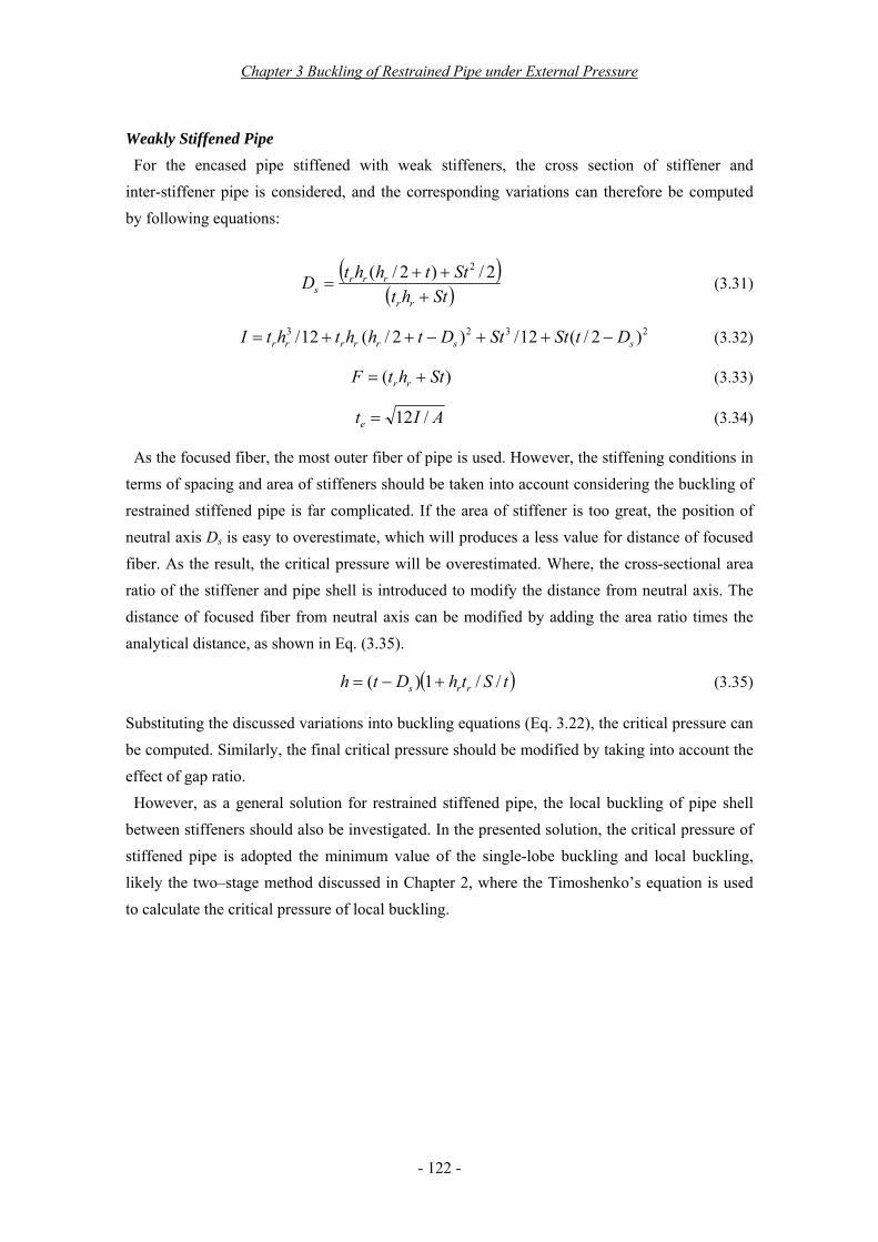
Chapter 3 Buckling of Restrained Pipe under External Pressure
- 122 -
Weakly Stiffened Pipe For the encased pipe stiffened with weak stiffeners, the cross section of stiffener and
inter-stiffener pipe is considered, and the corresponding variations can therefore be computed by following equations:
( )
( )SthtStthhtD
rr
rrrs +
++=
2/)2/( 2
(3.31)
2323 )2/(12/)2/(12/ ssrrrrr DtStStDthhthtI −++−++= (3.32)
)( SthtF rr += (3.33)
AIte /12= (3.34)
As the focused fiber, the most outer fiber of pipe is used. However, the stiffening conditions in terms of spacing and area of stiffeners should be taken into account considering the buckling of restrained stiffened pipe is far complicated. If the area of stiffener is too great, the position of neutral axis Ds is easy to overestimate, which will produces a less value for distance of focused fiber. As the result, the critical pressure will be overestimated. Where, the cross-sectional area ratio of the stiffener and pipe shell is introduced to modify the distance from neutral axis. The distance of focused fiber from neutral axis can be modified by adding the area ratio times the analytical distance, as shown in Eq. (3.35).
( )tSthDth rrs //1)( +−= (3.35)
Substituting the discussed variations into buckling equations (Eq. 3.22), the critical pressure can be computed. Similarly, the final critical pressure should be modified by taking into account the effect of gap ratio.
However, as a general solution for restrained stiffened pipe, the local buckling of pipe shell between stiffeners should also be investigated. In the presented solution, the critical pressure of stiffened pipe is adopted the minimum value of the single-lobe buckling and local buckling, likely the two–stage method discussed in Chapter 2, where the Timoshenko’s equation is used to calculate the critical pressure of local buckling.

Chapter 3 Buckling of Restrained Pipe under External Pressure
- 123 -
3.6.3 Verification of New Analytical Solution The new solution is verified using numerical analysis results. Where, the numerical results are
used, while the theoretical critical pressure is computed using the new analytical solution. The comparison between the numerical analysis results and analytical results was carried out,
and the comparing results in terms of ratio of analytical to numerical critical pressure are shown in Fig. 3.48, Fig. 3.49 and Fig. 3.50, respectively. Where, the comparing results are organized with respect to the thickness of pipe.
0.0
0.2
0.4
0.6
0.8
1.0
1.2
1.4
1.6
1.8
2.0
0.0001 0.001 0.01 0.1Δ/R
Ana
lytic
al / N
umer
ical
crit
ical
pre
ssur
e
S500tr10 S500tr20 S500tr30S1000tr10 S1000tr20 S1000tr30S1500tr10 S1500tr20 S1500tr30
Fig. 3.48 Comparison between analytical and numerical critical pressure ( t=5mm )
0.0
0.2
0.4
0.6
0.8
1.0
1.2
1.4
1.6
1.8
2.0
0.0001 0.001 0.01 0.1Δ/R
Ana
lytic
al / N
umer
ical
crit
ical
pre
ssur
e
S500tr10 S500tr20 S500tr30S1000tr10 S1000tr20 S1000tr30S1500tr10 S1500tr20 S1500tr30
Fig. 3.49 Comparison between analytical and numerical critical pressure ( t=10mm )

Chapter 3 Buckling of Restrained Pipe under External Pressure
- 124 -
0.0
0.2
0.4
0.6
0.8
1.0
1.2
1.4
1.6
1.8
2.0
0.0001 0.001 0.01 0.1Δ/R
Ana
lytic
al / N
umer
ical
crit
ical
pre
ssur
e
S500tr10 S500tr20 S500tr30S1000tr10 S1000tr20 S1000tr30S1500tr10 S1500tr20 S1500tr30
Fig. 3.50 Comparison between analytical and numerical critical pressure ( t=20mm )
From the comparing results as shown in Figs.3.48-3.50, the new solution can provide relatively sound results for various stiffened pipes, comparing with that from Jacobsen’s solution. All the ratio of theoretical to numerical critical pressure is less than the safety factor of 1.5. In addition, the results of all models with various pipes and stiffeners are agreeable in general can be found, although varies with the gap. However, the comparing results shown in Fig. 3.48 and Fig. 3.49 express in some divergence. The former is due to that the thin pipe occured local buckling for larger space stiffened cases and the critical pressure calculated through Timoshenko’s equation are used the theoretical value for local buckling, while the later is because of the results involving the weakly and rigidly stiffened pipe simultaneously.
Since the buckling of restrained stiffened pipe is complicated, which is related to not only the geometries of stiffened pipe and the initial gap but also the interaction between stiffeners and pipe, the perfect solution which can provide a completely consistent result is impossible. Therefore, the current analytical solution may be used to estimate a relative accurate critical pressure and provide a relative reasonable design. However, the design using the analytical solution should consider the safe factor in engineering practice.
Chapter 3 Buckling of Restrained Pipe under External Pressure
- 125 -
References 1) Vaughan, E.W.: Steel linings for pressure shafts in rock, J. Power Div., ASCE, Vol.82, pp.
9491-94940, 1956.
2) Cheney, J. A.: Pressure buckling of ring encased in cavity, J. Engrg. Mech. , Vol.97, No.2, pp.333-342, 1971.
3) Amstutz, E.: Buckling of pressure shaft and tunnel linings. Water Power, Vol. 22, pp. 391-399, Nov. 1970.
4) Jacobsen, S.: Buckling of circular rings and cylindrical tubes under external pressure, Water Power, Vol. 26, pp. 400-07, Dec., 1974.
5) El-Sawy, K.: Inelastic stability of tightly fitted cylindrical liners subjected to external uniform pressure, Thin-Walled Struct., Vol.39, No.9, pp.731–744, 2001.
6) El-Sawy, K. and Moore, I. D.: Stability of loosely fitted liners used to rehabilitate rigid pipes, J. Struct. Eng. , Vol. 124, No.11, pp.1350–1357, 1998.
7) Croll, J. G. A.: Buckling of cylindrical tunnel liners, Journal of Engineering Mechanics, Vol.127, No. 4, pp. 333-341, 2001.
8) Omara, A. M., Guice, L. K., Straughan, W. T., and Akl, F. A.: Buckling Models of Thin Circular Pipes Encased in Rigid Cavity, J. Engrg. Mech., Vol. 123, No. 12, pp. 1294-1301, 1997.
9) Yamamoto, Y., and Matsubara, N.: Buckling of a cylindrical shell under external pressure restrained by an outer rigid wall, Proc., Collapse and Buckling, Struct. Theory and Practice Symp., Cambridge University Press, London, U.K., 493–504, 1982.
10) Berti, D., Stutzman, R., Lindquist, E., and Eshghipour, M.: Buckling of steel tunnel liner under external pressure, J. Energy Eng., Vol.124, No.3, pp.55–89, 1998.
11) JSCE: Design Standard for Steel structure,Part B Special structure,JSCE Pub., 1987. 12) JHJPA: Technology Specification of Water Duct and Steel Pipe, pp.44-65, JHJPA Pub.,
2001.
13) Glock, D.: Post-critical Behavior of a Rigidly Confined Circular Tube under External Water Pressure and Temperature Caused Extension, Stahlbau, 46 (7), pp. 212-217, 1977.
14) Boot, J. C.: Elastic buckling of cylindrical pipe linings with small imperfections subject to external pressure, Trenchless Technology Res., Vol.12, Nos.1-2, pp.3-15, 1998.
15) Boot, J. C. & Javadi, A.A.: Experimental determination of buckling capacities of cured-in-place, pipe linings., 11th International Conference on Experimental Mechanics, Oxford, UK, Aug. 1998.
16) Aggarwal, S. C. and Cooper, M.J. : External Pressure Testing of ‘Insituform’ Linings, Internal Report, Coventry (Lanchester) Polytechnic, UK, 1984.
Chapter 3 Buckling of Restrained Pipe under External Pressure
- 126 -
17) Lu, K. H., and Zhang, J. Q. : Collapse resistance modeling of encased pipes, Buried Plastic Pipe Technology, Vol.2, pp. 97-110, ASTM STP1222, 1994.
18) Marc Analysis Research Corp.: Contact analysis, Msc.Marc 2005, Vol. A,B,C. Marc Analysis Research Corp, 2005.
Related Documents