Chapter 2: Problem Solutions - Naval Postgraduate Schoolfaculty.nps.edu/.../solutions/Solutions_Chapter2.pdf · Chapter 2: Problem Solutions Discrete Time Processing of Continuous

Chapter 2: Problem SolutionsDiscrete Time Processing of Continuous Time Signals

Sampling

à Problem 2.1.

Problem:

Consider a sinusoidal signal

xt 3cos1000t 0.1and let us sample it at a frequency Fs 2kHz.

a) Determine and expression for the sampled sequence xn xnTs and determine its Discrete Time Fourier Transform X DTFTxn;

b) Determine XF FTxt;

c) Recompute X from the XF and verify that you obtain the same expression as in a).

Solution:

a) xn xt tnTs 3cos0.5n 0.1 . Equivalently, using complex exponentials,

xn 1.5ej0.1ej0.5n 1.5ej0.1ej0.5n

Therefore its DTFT becomes

X DTFTxn 3ej0.1 2 3ej0.1 2 with

b) Since FTej2F0t F F0 then

XF 1.5ej0.1F 500 1.5ej0.1F 500for all F .

c) Recall that X DTFTxn and XF FTxt are related as

X Fs k

XF kFs FFs2

with Fs the sampling frequency. In this case there is no aliasing, since all frequencies are contained within Fs 2 1kHz . Therefore, in the interval we can write

X FsXF FFs2

with Fs 2000Hz . Substitute for XF from part b) to obtain

X 20001.5ej0.12000 2 500 1.5ej0.12000 2 500Now recall the property of the "delta" function: for any constant a 0 ,

at 1a ta Therefore we can write

X 3ej0.1 2 3ej0.1 2 same as in b).

à Problem 2.2.

Problem

Repeat Problem 1 when the continuous time signal is

xt 3cos3000t

Solution

Following the same steps:

a) xn 3cos1.5n . Notice that now we have aliasing, since F0 1500Hz Fs2 1000Hz . Therefore, as shown in the figure below, there is an aliasing at Fs F0 2000 1500Hz 500Hz . Therefore after sampling we have the same signal as in Problem 1.1, and everything follows.

2 Solutions_Chapter2[1].nb

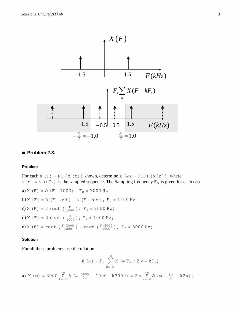
)(FX

)(kHzF5.15.1

k

ss kFFXF )(

)(kHzF5.15.1 5.05.0

0.12 sF0.12 sF

à Problem 2.3.

Problem

For each XF FTxt shown, determine X DTFTxn , where xn xnTs is the sampled sequence. The Sampling frequency Fs is given for each case.

a) XF F 1000 , Fs 3000Hz;

b) XF F 500 F 500 , Fs 1200Hz

c) XF 3rect F1000 , Fs 2000Hz;

d) XF 3rect F1000 , Fs 1000Hz;

e) XF rect F30001000 rect F30001000 , Fs 3000Hz;

Solution

For all these problems use the relation

X Fsk

X Fs 2 kFs

a) X 3000 k

30002 1000 k3000 2

k

23 k2;

Solutions_Chapter2[1].nb 3

b) X 1200 k

12002 500 k1200 12002 500 k1200

2 k

0 k2 0 k2

0 2 500 1200 1.2;

c) X 20003 k

rect 200021000 k 20001000 6000

k

rect k2 shown

below.

2

2 22

)(X

d) X 10003 k

rect 100021000 k 10001000 3000

k

rect k22 shown below

22

)(X

e) X 3000 k

rect 3000230001000 k 30001000 rect 3000230001000 k 30001000

3000 k

rect 32 3 3k rect 32 3 3k

6000 k

rect k223

shown below.

22

)(X

62 6

2

6000

4 Solutions_Chapter2[1].nb

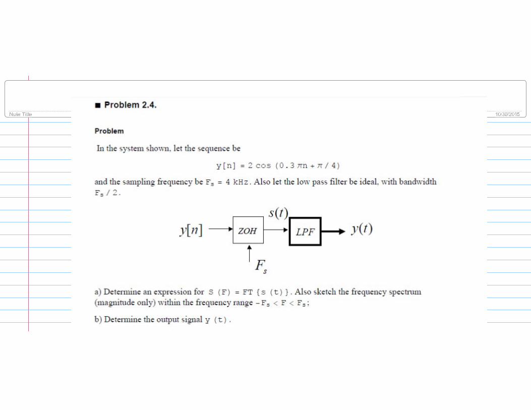
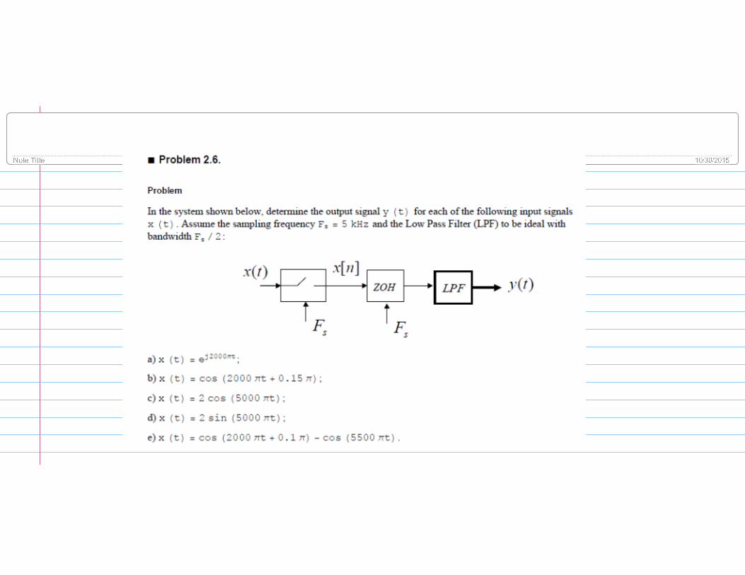
ZOH LPF

][nx

sFsF

)(tx ][nx

and let the sampling frequency be Fs 2000Hz .

a) Determine the continuous time signal yt after the reconstruction.

b) Notice that yt is not exactly equal xt . How could we reconstruct the signal xt exactly from its samples xn?

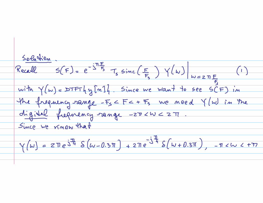
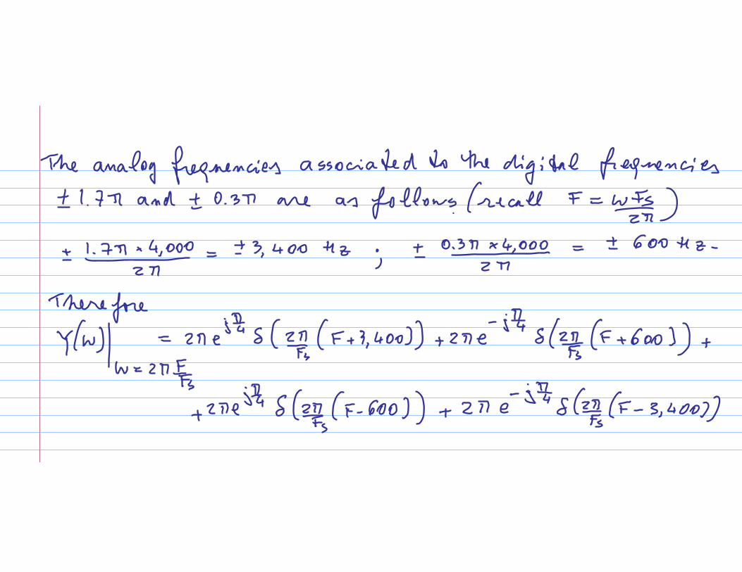
Solution

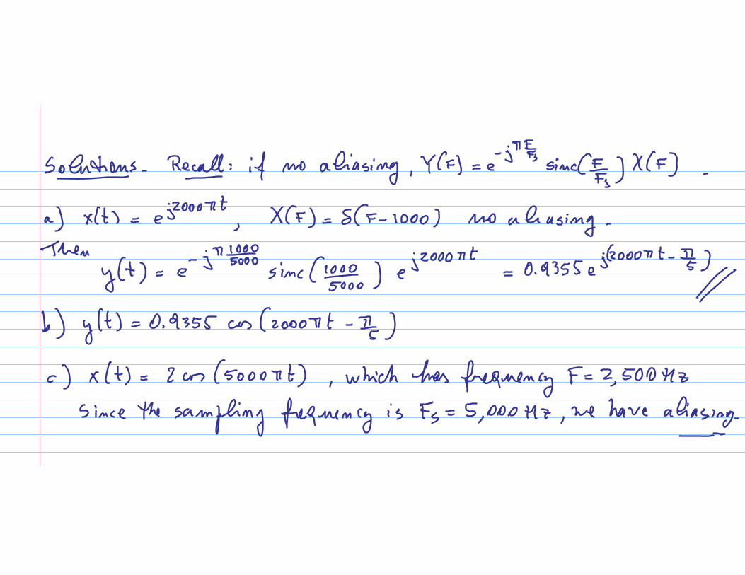
a) Recall the formula, in absence of aliasing,

YF ejFFs sinc FFsXF

with Fs 2000Hz being the sampling frequency. In this case there is no aliasing, since the maxi-mum frequency is 750Hz smaller than Fs 2 1000Hz . Therefore, each sinusoid at frequency F has magnitude and phase scaled by the above expression. Define

GF ej F2000 sin F2000 F2000

which yields

G250 0.9745ej0.392, G500 0.9003ej0.785, G750 0.784ej1.178

Finally, apply to each sinusoid to obtain.

yt 20.9745cos500t 0.392 30.9003sin1000t 0.785 0.784cos1500t 1.178

b) In order to compensate for the distortion we can design a filter with frequency response 1 GF , when Fs2 F Fs2 .The magnitude would be as follows

Solutions_Chapter2[1].nb 7

e) the term cos2 2750 t has aliasing, since it has a frequency above 2500Hz. From the figure, the aliased frequency is

)(FX

)( sFFX )( sFFX )(kHzF

75.275.2

25.2575.2

Faliased 5.00 2.75 2.25kHz . Therefore it is as if the input signal were xt cos2000t 0.1 cos4500t . This yields G1000 0.935ej0.628 and G2250 0.699ej0.393 , and finally

yt 0.935cos2000t 0.1 0.628 0.699cos4500t 1.41372

à Problem 2.7.

Problem

Suppose in the DAC we want to use a linear interpolation between samples, as shown in the figure below. We can call this reconstructor a First Order Hold, since the equation of a line is a polynomial of degree one.

FOH

][ny

sF

)(ty][ny

)(ty

sTn

a) Show that yt n

xngt nTs , with gt a triangular pulse as shown below;

Solutions_Chapter2[1].nb 9

sTsT

1)(tg

tb) Determine an expression for YF FTyt in terms of Y DTFTyn and GF FTgt;

c) In the figure below, let yn 2cos0.8n , the sampling frequency Fs 10kHz and the filter be ideal with bandwidth Fs 2 . Determine the output signal yt .

FOH LPF

sF

)(ty][ny

Solution

a) From the interpolation yt n

xngt nTs and the definition of the interpolating

function gt we can see that yt is a sequence of straight lines. In particular if we look at any interval nTs t n 1Ts it is easy to see that only two terms in the summation are nonzero, as

yt xngt nTs xn 1gt n 1Ts , for nTs t n 1Ts

This is shown in the figure below. Since gTs 0 we can see that the line has to go through the two points xn and xn 1 , and it yields the desired linear interpolation.

10 Solutions_Chapter2[1].nb

snT sTn )1(

)(][ snTtgnx ))1((]1[ sTntgnx

)(ty

t

Interpolation by First Order Hold (FOH)

b) Taking the Fourier Transform we obtain

YF FTyt n

xnGFej2FnTs

GFX 2FFs

where GF FTgt . Using the Fourier Transform tables, or the fact that (easy to verify)

gt 1Tsrect tTs

rect tTs

we determine GF Tssinc FFs2 , since FTrect tTs

Tssinc FFs .

à Problem 2.8.

Problem

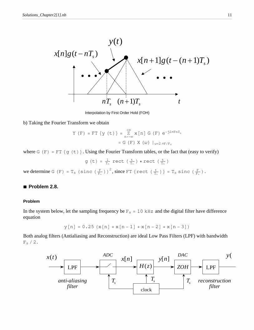
In the system below, let the sampling frequency be Fs 10kHz and the digital filter have difference equation

yn 0.25xn xn 1 xn 2 xn 3Both analog filters (Antialiasing and Reconstruction) are ideal Low Pass Filters (LPF) with bandwidth Fs 2 .

x t( ) x n[ ] y n[ ]y(

H z( )

ADC DAC

ZOH

clock

Ts TsTs

LPF LPF

anti-aliasingfilter

reconstructionfilter

Solutions_Chapter2[1].nb 11

a) Sketch the frequency response H of the digital filter (magnitude only);

b) Sketch the overall frequency response YF XF of the filter, in the analog domain (again magnitude only);

c) Let the input signal be

xt 3cos6000t 0.1 2cos12000tDetermine the output signal yt .

Solution.

a) The transfer function of the filter is Hz 0.251 z1 z2 z3 0.25 1z41z1 , where

we applied the geometric sum. Therefore the frequency response is

H Hz zej 0.25 1ej41ej 0.25 ej1.5 sin2sin 2

whose magnitude is shown below.

b) Recall that the overall frequency response is given by

YFXF H 2FFsejFFs sinc FFs

In our case Fs 10kHz , and therefore we obtain

4000 2000 2000 4000F

0.2

0.4

0.6

0.8

1

1.2

1.4

YFXF

12 Solutions_Chapter2[1].nb

c) The input signal has two frequencies: F1 3kHz Fs 2, and F2 6kHz Fs 2 , with Fs 10kHz the sampling frequency. Therefore the antialising filter is going to stop the second frequency, and the overall output is going to be

yt 30.156 cos6000 t 0.1 0.1 0.467745 cos6000 t 0.62832

since, at F 3kHz , YF XF 0.156ej0.1 .

Quantization Errors

à Problem 2.9

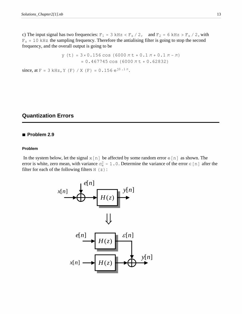
Problem

In the system below, let the signal xn be affected by some random error en as shown. The error is white, zero mean, with variance e

2 1.0. Determine the variance of the error n after the filter for each of the following filters Hz :

)(zH][nx

][ne][ny

)(zH][nx][ny

][n)(zH

][ne

Solutions_Chapter2[1].nb 13

a) Hz an ideal Low Pass Filter with bandwidth 4;

b) Hz zz0.5 ;

c) yn 14 sn sn 1 sn 2 sn 3 , with sn xn en;

d) H e , for .

Solution.

Recall the two relationships in the frequency and time domain:

2 12

H

2 d

e

2

hn 2 e2

a) 2 12

H

2 d

e

2 12

4

4

d e

2 14 e2 ;

b) the impulse response in this case is hn 0.5nun therefore

2

hn 2 e2

0

0.52n e

2 110.25 e2 43 e

2

c) in this case n 14 en en 1 en 2 en 3 . Therefore the impulse response is

hn 14 n n 1 n 2 n 3and therefore

2 n0

3 142 e

2 4 116 e2 14 e

2

d) 2

12

ewde

2 0.3045 e2

à Problem 2.10.

Problem

A continuous time signal xt has a bandwidth FB 10kHz and it is sampled at Fs 22kHz, using 8bits/sample. The signal is properly scaled so that xn 128 for all n .

a) Determine your best estimate of the variance of the quantization error e2 ;

b) We want to increase the sampling rate by 16 times. How many bits per samples you would use in order to maintain the same level of quantization error?

14 Solutions_Chapter2[1].nb

Solution

a) Since the signal is such that 128 xn 128 it has a range VMAX 256. If we digitize it with Q1 8 bits. we have 28 256 levels of quantization. Therefore each level has a range VMAX 2Q1 256256 1 . Therefore the variance of the noise is e

2 112 if we assume uniform distribution.

b) If we increase the sampling rate as Fs2 16 Fs1 , the number of bits required for the same quantization error becomes

Q2 Q1 12 log2Fs1Fs2

8 12 4 6 bitssample

Solutions_Chapter2[1].nb 15