Working paper 4 28 June 2016 UNITED NATIONS ECONOMIC COMMISSION FOR EUROPE CONFERENCE OF EUROPEAN STATISTICIANS Seminar on poverty measurement 12-13 July 2016, Geneva, Switzerland Item 3: Measurement challenges in consumption and income poverty Chapter 2: Monetary Poverty GUIDE ON POVERTY MEASUREMENT Chapter leader: ONS, United Kingdom Draft 28 June 2016 Section A: Concepts & Methods 1. Introduction As set out in the previous chapter, by far the most commonly used approach to measuring poverty is the use of monetary indicators, usually based on low income or consumption, as a proxy for low material living standards. Income refers to the ongoing flow of economic resources that a household receives over time. It includes wages and salaries and money earned through self-employment as well as private pensions, investments and other non-government sources and cash benefits/social transfers. The main international standards describing the concepts and components of household income in micro statistics are contained in the Canberra Group Handbook on Household Income Statistics (UNECE, 2011). Income is important in this context as it allows people to satisfy their needs and pursue many other goals that they deem important to their lives. Those with low incomes typically have a restricted capacity to consume the goods and services they need to participate fully in the society in which they live. Consumption is the use of goods and services to directly satisfy a person’s needs and wants, whilst consumption expenditure is the value of consumption goods and services paid for by a household. Considered simply, and everything else being equal, people with lower levels of consumption or consumption expenditure can be regarded as having a lower level of current economic well-being. Many economists would argue consumption is a more important determinant of economic well-being than income alone. Indeed, Brewer and O’Dea (2012) and others (see Noll, 2007 for a review) argue that it is preferable to consider the distribution of consumption rather than income on both theoretical and pragmatic grounds. However, there are a number of reasons why many countries prefer income based poverty measures. The pros and cons of each approach are discussed later in this chapter.

Welcome message from author
This document is posted to help you gain knowledge. Please leave a comment to let me know what you think about it! Share it to your friends and learn new things together.
Transcript
Working paper 4
28 June 2016
UNITED NATIONS
ECONOMIC COMMISSION FOR EUROPE
CONFERENCE OF EUROPEAN STATISTICIANS
Seminar on poverty measurement
12-13 July 2016, Geneva, Switzerland
Item 3: Measurement challenges in consumption and income poverty
Chapter 2: Monetary Poverty
GUIDE ON POVERTY MEASUREMENT
Chapter leader: ONS, United Kingdom
Draft 28 June 2016
Section A: Concepts & Methods
1. Introduction
As set out in the previous chapter, by far the most commonly used approach to measuring poverty is
the use of monetary indicators, usually based on low income or consumption, as a proxy for low
material living standards.
Income refers to the ongoing flow of economic resources that a household receives over time. It
includes wages and salaries and money earned through self-employment as well as private pensions,
investments and other non-government sources and cash benefits/social transfers. The main
international standards describing the concepts and components of household income in micro
statistics are contained in the Canberra Group Handbook on Household Income Statistics (UNECE,
2011). Income is important in this context as it allows people to satisfy their needs and pursue many
other goals that they deem important to their lives. Those with low incomes typically have a restricted
capacity to consume the goods and services they need to participate fully in the society in which they
live.
Consumption is the use of goods and services to directly satisfy a person’s needs and wants, whilst
consumption expenditure is the value of consumption goods and services paid for by a household.
Considered simply, and everything else being equal, people with lower levels of consumption or
consumption expenditure can be regarded as having a lower level of current economic well-being.
Many economists would argue consumption is a more important determinant of economic well-being
than income alone. Indeed, Brewer and O’Dea (2012) and others (see Noll, 2007 for a review) argue
that it is preferable to consider the distribution of consumption rather than income on both theoretical
and pragmatic grounds. However, there are a number of reasons why many countries prefer income
based poverty measures. The pros and cons of each approach are discussed later in this chapter.
Working paper 4
Page 2
Monetary poverty measures can broadly be divided into two types: absolute and relative. Absolute
poverty lines represent the value of a set level of resources necessary to provide a given minimum
standard of well-being. Perhaps the most widely recognised absolute measure is the $1.90 a day (in
2011 prices) line for extreme poverty, which has been established by the World Bank. However,
different absolute poverty lines are used by many other countries. For example, the United States
Census Bureau uses an absolute poverty threshold, which stood at $12,071 a year in 2014 for a single
adult household.
By contrast, relative measures utilise poverty lines that are set in relation to the average situation
within a society. Typically, these lines are based on either mean or median income or expenditure.
The rationale for such an approach comes from a definition of poverty that moves beyond absolute
destitution to considering individuals capacity to participate fully in society. An example of such a
definition is that set out by the European Council in 1975, which states that “People are said to be
living in poverty if their income and resources are so inadequate as to preclude them from having a
standard of living considered acceptable in the society in which they live.” This definition is
operationalised through the European Commission’s indicator based on the proportion of individuals
living in households with equivalised disposable incomes below 60% of the national median. The
OECD use a similar approach in their statistics, though the main income poverty threshold used is
50% of the national median.
Despite their usefulness and ubiquity, there are a number of limitations to monetary indicators of
poverty. Importantly, low household incomes or low levels of consumption do not necessarily imply a
low standard of living. A household with a low income may be able to achieve a high standard of
living through the use of savings or debt (based on an expectation of higher income in the future).
Additionally, levels of wealth, which are the third primary component of economic well-being are not
typically taken account of in monetary poverty indicators. Similarly, and depending on the thresholds
used, low levels of consumption may in part reflect individual choices or non-monetary constraints
(e.g. elderly people with physical limitations, such as lack of mobility, who may have low levels of
consumption despite adequate financial resources).
More generally, monetary measures based on private household resources do not necessarily reflect
access to basic services such as education, healthcare, water and infrastructure. Multidimensional and
subjective measures of poverty, which do attempt to take account of such unmet basic needs, are
described in subsequent chapters.
Such limitations of monetary indicators are often recognised in the way they are described in
publications both by national governments and international organisations. For example, the UK
Department for Work and Pensions refers to “relative low income” in their published statistics, whilst
Eurostat report on ”at-risk-of-poverty rates” (DWP, 2015; Eurostat, 2015).
2. Unit of observation
In producing data on income or consumption, the normal unit of observation should be the household
(or family), for both practical and conceptual reasons. If data are collected through household surveys,
it is often impractical and expensive to collect data in detail from all members of the household. More
importantly, it is often very difficult or impossible to allocate economic flows to single individuals
within the household or family unit. For example, certain types of income from social protection
payments may be allocated at the family, rather than the individual level. Similarly, it is challenging
to allocate to individuals consumption expenditure that is carried out on behalf of the whole
household.
The need to measure income at the household level is perhaps best illustrated in the case of families
with children. The children will typically have few, if any, economic resources of their own and rely
predominantly on intra-household transfers from their parents. The measurement of such intra-
household transfers is, at best, difficult, but by considering the household as the basic statistical unit,
the need to do so is removed.
The measurement of economic resources at the household (or family) level presents a number of
issues, however. First, it is generally necessary to assume that resources are shared equitably amongst
Working paper 4
Page 3
all members of the household. In reality, there may be an unequal distribution of resources between
men and women or between different generations within the household. The limitations of this
assumption have been widely recognised for some time (Jenkins, 1991) and research has attempted to
better understand intra-household sharing of resources and its implications for poverty statistics (for
example, Ponthieux, 2013). However, the substantial methodological and data collection challenges
have limited progress and mean that this assumption remains integral to almost all published poverty
statistics.
A second issue is that in determining whether a given level of economic resources at a household is
sufficient to meet basic needs or allow participation in society, the number of people living within the
household clearly needs to be taken into account. The simplest approach to dealing with this is to
consider household income or consumption per capita. This is the method used for the World Bank’s
$1.90/day and $3.10/day poverty lines. However, such an approach fails to account for economies of
scale which can occur within households. For example, a household of three adults is likely to need a
higher income to enjoy the same standard of living as a single person household, but not necessarily
three times the income. Additionally, the per capita approach also assumes that the level of resources
needed by, for example, a 40 year old woman is the same as that needed by a 8 year old boy. To
account for these points, so-called equalivalisation (or equivalence) scales are often used. These are
discussed later in this chapter.
3. Unit of analysis
Although income and consumption are both normally measured at the household level, this does not
mean that households should be the statistical unit used for poverty analysis. Poverty is something
that is experienced by individuals, and the aim of policy is to improve the position of those individual
citizens, whether children, working-age or in retirement. As a consequence, poverty statistics should
be reported at the individual level, with the indicators used describing, for example, the number of
individuals in a population living in households below the poverty line.
4. Household definition
The Canberra Handbook (p 64) sets out a definition of a household as:
Either (a) a person living alone in a separate housing unit or who occupies, as a lodger, a separate
room (or rooms) of a housing unit but does not join with any of the other occupants of the housing
unit to form part of a multi-person household or (b) a group of two or more persons who combine to
occupy the whole or part of a housing unit and to provide themselves with food and possibly other
essentials for living. The group may be composed of related persons only or of unrelated persons or
of a combination of both. The group may also pool their income.
This definition is based on the definition of a private household used in the Conference of European
Statisticians Recommendations for the 2010 Censuses of Population and Housing (UNECE, 2006)
and should be considered the recommended benchmark for poverty measurement.
In line with the CES/UNECE guidelines, “Place of usual residence” should be used as the basis for
household membership. The guidelines provide recommendations for a number of special cases. For
example, those work work away from family home during the week and return at weekends (place of
usual residence is family home), school children away from home during term-time (place of usual
residence is family home), or a child alternating between multiple residences (place of usual residence
should be the address where most time is spent).
In all cases, those involved in the measurement of poverty should include within the metadata the
definition of household used and the approach for the allocation of individuals, particularly where this
standard approach has not been followed.
Working paper 4
Page 4
It is important to note the distinction between households and families. A family is defined as those
members of the household who are related, to a specified degree, through blood, adoption or marriage.
The degree of relationship used in determining the limits of the family in this sense is dependent upon
the uses to which the data are to be put and there is no universally agreed statistical definition which is
used worldwide. However, in all cases it is true that a family cannot comprise more than one
household. A household, however, can contain more than one family.
Individuals and families not living in private households provide a practical challenge for the
compilation of poverty statistics and these are discussed in the next section, along with other
population sub-groups that are sometimes omitted from official statistics.
5. Population coverage
Poverty statistics should, of course, in theory all of the population or sub-population of interest.
However, as with all social statistics, the practical limitations of data collection mean this is not
always straightforward or even possible. This is a particular issue for the measurement of poverty as it
is often the case that poverty is more prevalent amongst these hard to reach groups.
a. Communal establishments
Communal establishments or institutional households comprise persons whose need for shelter and
subsistence are being provided by an institution. An institution is understood to be a legal body for the
purpose of long-term inhabitation and provision of services to a group of persons. Institutions usually
have common facilities shared by the occupants. The great majority of institutional households are
considered to fall into the following categories: residences for students; hospitals, convalescent
homes, old people’s homes, etc.; assisted-living facilities and welfare institutions; military barracks;
correctional and penal institutions; religious institutions; and worker dormitories.
The vast majority of household statistics collected through social surveys do not cover communal
establishments, largely due to the practical difficulties associated with data collection, though there
are additional challenges associated with the definition of household income or consumption in such
establishments. The survey of country practices carried out for the latest edition of the Canberra
Handbook revealed that none of the responding countries’ income micro-statistics covered communal
establishments such as university halls of residence or institutions for long-term care.
b. Homeless
Those with no usual place of residence are also not covered by standard household surveys designed
to measure income or consumption. However, they also typically represent some of the poorest and
most vulnerable individuals in society. Homeless households include those living in temporary or
insecure accommodation, as well as those who are sleeping rough.
Whilst it may not be possible to include homeless households within standard household surveys, it is
important to consider alternative ways in which such households can be captured in information about
poverty. The approach used is likely to vary across countries according to the information available.
In Nordic countries, for example, data on population registers may be of some use. Elsewhere, it may
be possible to make use of information collected by local government or other agencies, as well as the
voluntary sector.
Italy’s experience of collecting data for the homeless population is described in Box 2.1.
Working paper 4
Page 5
Box 2.X Italy experience of collecting data for homeless population.
The European Observatory on homelessness tried to construct a definition of homelessness and housing
exclusion that, on the one hand, was wider than the simple photograph of homeless people and that
represented, on the other hand, a compromise between the different national approaches (Amore et al.,
2011).
There are numerous definitions of homeless person coming from different operational and scientific fields;
in the international literature, the condition of homelessness is defined from time to time with terms such
as homeless, roofless, clochard, etc., according to the meanings and implications which do not always
coincide. However, each definition includes, structurally, four recurrent elements - the
multidimensionality, the progressivity of the marginalization path, the exclusion from welfare benefits and
the difficulty in structuring and maintaining meaningful relationships – identifying the homeless person as
a subject in a state of material and immaterial poverty, bearer of a uncomfortable, dynamic and multi-
faceted complex distress.
The result of this effort is the ETHOS definition (European Typology on Homelessness and Housing
Exclusion), published for the first time in 2004, that is not a final construct, but is intended to be annually
revisited to adapt incrementally to the realities of the member countries.
The purpose of the instrument is, in fact, to provide a common operational definition to various European
countries, useful for collecting comparable data on the phenomenon of housing poverty in its various
shades. The homelessness is a transitory and dynamic condition, not a static experience, and it is necessary
to define procedures able to grasp not only the concrete manifestation, but also the vulnerability factors.
A strategy to obtain information on homelessness should not, therefore, be restricted to the monitoring of
the number of homeless people, but it should also obtain and provide information on their profiles and life
experiences, trying to give even useful elements to improve the services aiming to prevent and relieve
distress.
It therefore becomes essential to a) define a set of variables for meaningful comparisons between different
national and international realities, to improve, at the same time, understanding homelessness and the
profiles of the mutant population of homeless persons; b) collect data on potential and actual services for
people with housing distress.
A series of recommendations have been developed, aimed at assisting the national authorities, to improve
skills in gathering information on homelessness and to identify the necessary actions and initiatives, at
national and European level.
The above ETHOS definition, by detailing, identifies three domains to define the concept of home, the
absence of which outlines a condition of housing poverty: "having a decent dwelling (or space) adequate to
meet the needs of the person and his/her family (physical domain); being able to maintain privacy and
enjoy social relations (social domain); and having exclusive possession, security of occupation and legal
title (legal domain)”.
Working paper 4
Page 6
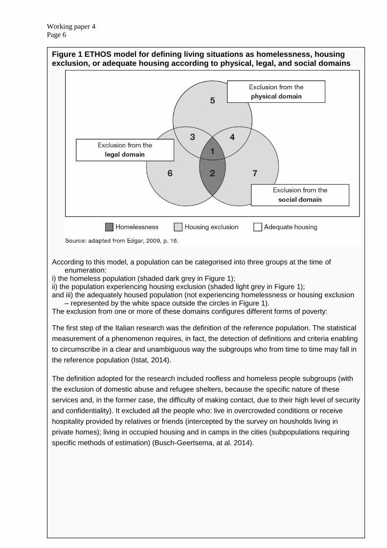
Figure 1 ETHOS model for defining living situations as homelessness, housing
exclusion, or adequate housing according to physical, legal, and social domains
According to this model, a population can be categorised into three groups at the time of enumeration:
i) the homeless population (shaded dark grey in Figure 1); ii) the population experiencing housing exclusion (shaded light grey in Figure 1); and iii) the adequately housed population (not experiencing homelessness or housing exclusion
– represented by the white space outside the circles in Figure 1). The exclusion from one or more of these domains configures different forms of poverty: The first step of the Italian research was the definition of the reference population. The statistical
measurement of a phenomenon requires, in fact, the detection of definitions and criteria enabling
to circumscribe in a clear and unambiguous way the subgroups who from time to time may fall in
the reference population (Istat, 2014).
The definition adopted for the research included roofless and homeless people subgroups (with
the exclusion of domestic abuse and refugee shelters, because the specific nature of these
services and, in the former case, the difficulty of making contact, due to their high level of security
and confidentiality). It excluded all the people who: live in overcrowded conditions or receive
hospitality provided by relatives or friends (intercepted by the survey on housholds living in
private homes); living in occupied housing and in camps in the cities (subpopulations requiring
specific methods of estimation) (Busch-Geertsema, at al. 2014).
Working paper 4
Page 7
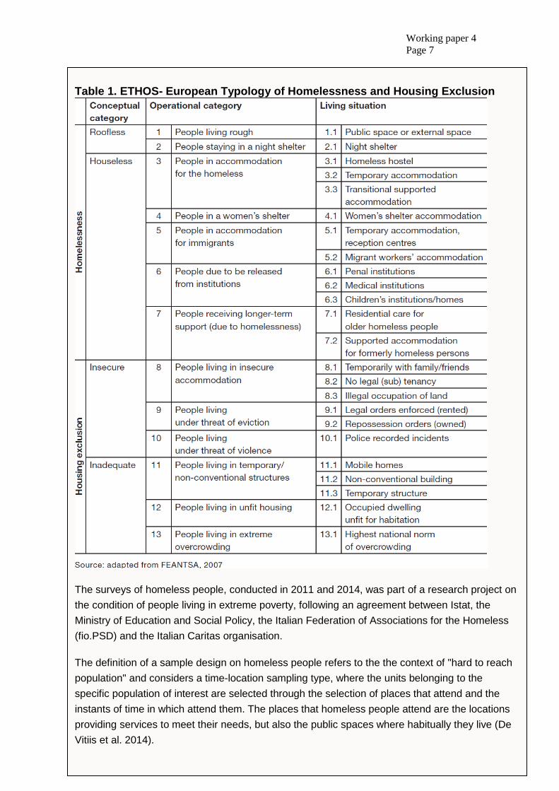
Table 1. ETHOS- European Typology of Homelessness and Housing Exclusion
The surveys of homeless people, conducted in 2011 and 2014, was part of a research project on
the condition of people living in extreme poverty, following an agreement between Istat, the
Ministry of Education and Social Policy, the Italian Federation of Associations for the Homeless
(fio.PSD) and the Italian Caritas organisation.
The definition of a sample design on homeless people refers to the the context of "hard to reach
population" and considers a time-location sampling type, where the units belonging to the
specific population of interest are selected through the selection of places that attend and the
instants of time in which attend them. The places that homeless people attend are the locations
providing services to meet their needs, but also the public spaces where habitually they live (De
Vitiis et al. 2014).
Working paper 4
Page 8
For the research, two alternative solutions were considered: the first involved the detection at
canteens and night shelters (such as key forums where intercepting, with a high frequency, a
large number of homeless people); the second at the night shelter services and street units. Both
solutions showed some limitations related to the incomplete coverage of the phenomenon and to
the risk of multiple counts.
In the night shelter and canteens the multiple counting issue is determined by repeated
attendance of the same services, but it could be solved with a suitable detection pattern or
through the identification of people surveyed. The detection of the phenomenon in the public
spaces (through the street units) instead poses a further problem due to the difficulty of
administering a long and complex questionnaire that would allow to keep under control the risk of
multiple counts.
Both the solutions do not guaranteed the full coverage of the phenomenon: in the first because of
the failure to capture the part of homeless people living in public spaces and not using neither
night shelter or canteen services; in the second due to the fact that the outdoor units not
guarantee full coverage of the territory.
The choice was oriented towards the first solution in the light of the fact that the purpose the
research was the estimation of the number of homeless people and , at the same time, the
outlining of profiles in terms of socio-demographic and economic characteristics (requiring an
articulate interview). The survey on homeless people was, therefore, conducted at all centers
providing canteen and night shelters services. The choice of services was essential not only to
define the places to intercept the homeless, but also to prepare the sampling frame.
In synthesis, the survey was conducted using a different methodology to that usually applied in
households surveys of households and individuals, given the lack of any pre- existing list of the
population in question. According to the methodology based on the theory of indirect sampling, a
population, indirectly linked to the target population, was considered as a sampling base. In this
specific case, for the study of homeless people, the sample base was represented by the
services offered (meals distributed and accommodation places) by certain types of providers
(canteens and night - time shelters).
In the first survey, conducted in 2011, the list of services was constructed in two phases, prior to
the survey of homeless people: i) a census of the organisations offering services to the
homeless in the main Italian municipalities; ii) an in-depth survey of the services provided. The
services census was conducted in 158 Italian municipalities, selected according to their
demographic size (Istat, 2011, 2013).
The survey of homeless people represents the third phase of the process, and was conducted
over a period of thirty days, in order to include a larger number of service users.
The sample design randomly distributed the interviews over the opening hours and days of the
centres in the month of reference, and included all the centres involved in the two previous
phases. A two - phase sample plan was used, the first stage of which involved selecting the
survey days, and the second the services provided.
Working paper 4
Page 9
The number of homeless people was estimated by measuring the number of links between each
interviewed individual and the services used in the week immediately preceding the interview:
this was done by filling a weekly diary recording the individual's visits to the various centres on
the reference list. In this way, the estimates were accurate and not affected by distortions
introduced by double counting.
The operation involved 43 territorial contacts and 773 interviewers, who aimed to interview 4,963
homeless people; 7,364 contacts were made, resulting in 4,696 valid interviews. We succeeded
in interviewing 94.6% of the theoretical sample, with slightly higher results for night - time shelters
(96.5% against 93.3% in canteens); more than half (53%) of the 2,668 contacts which failed to
result in an interview were due to the fact that the person contacted was not homeless; a further
27.8% refused to be interviewed and 13% had already been interviewed; the remaining 6.1% of
interviews were interrupted.
The follow-up survey, conducted in 2014, required three essential steps: i) updating the archive
of canteen and night shelter services; ii) preparing the sampling plan and the tools for the survey
on homeless persons; iii) conducting the survey (Istat, 2015).
The operation involved 65 local contacts and 516 interviewers, who aimed to interview 4,864
homeless persons. The number of contacts equalled 7,322 and led to carrying out 4,726 valid
interviews. The sample size reached equalled 97.2% of the theoretical one, and was slightly
higher for night shelters (97.7% against 96.8% for canteens). In almost one half of the cases, the
2,596 contacts that produced a non-interview (47.1%), are due to the fact that the contacted
person was not homeless; an additional 46.7% were refusals or interrupted interviews, and the
remaining 6.3% regarded persons already interviewed.
Both the surveys were able to estimate, describe and monitor the population of homeless people
which used a canteen or night-time accommodation service at least once in the 158 Italian
municipalities and in the period in which the survey was conducted.
In 2014, it is estimated that 50,724 homeless persons, in the months of November and
December 2014, used at least one canteen or night shelter in the 158 Italian municipalities where
the survey was carried out. This amount corresponds to the 2.43 per thousand of the population
regularly registered with the municipalities taken into consideration by the survey, a value higher
than in 2011, when it was 2.31 per thousand (47,648 persons).
However, the population observed by the survey also includes individuals not entered in the civil
registry, or residing in municipalities other than those where they live. About two thirds of
homeless persons (68.7%) declare they are entered in the civil registry of an Italian municipality –
a figure that falls to 48.1% among foreign nationals and reaches 97.2% among Italians.
In comparison with 2011, the main features of homeless persons were confirmed: they are
mostly men (85.7%), foreigners (58.2%), under 54 years of age (75.8%) – although, following the
decline in foreigners under 34 years of age, the average age has seen a slight increase (from
42.1 to 44.0) – or with a low level of education (only one third hold at least a secondary school
diploma).
Working paper 4
Page 10
Growing in comparison with the past is the percentage of those living alone (from 72.9% to
76.5%), to the detriment of those living with a partner or child (from 8% to 6%); slightly more than
one half (51%) declare they have never been married.
The duration of the condition of homelessness has also increased in comparison with 2011:
those who have been homeless for less than three months have declined from 28.5% to 17.4%
(those who have been homeless for less than 1 month have been halved), while the share of
those who have been homeless for more than two years (rising from 27.4% to 41.1%) and for
more than 4 years (rising from 16% to 21.4%) has increased.
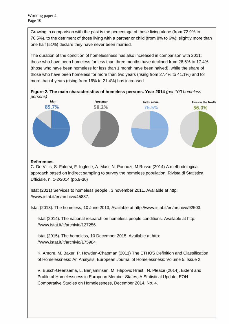
Figure 2. The main characteristics of homeless persons. Year 2014 (per 100 homeless persons)
Man
85.7% Foreigner
58.2% Lives alone
76.5% Lives in the North
56.0%
References C. De Vitiis, S. Falorsi, F. Inglese, A. Masi, N. Pannuzi, M.Russo (2014) A methodological
approach based on indirect sampling to survey the homeless population, Rivista di Statistica
Ufficiale, n. 1-2/2014 (pp.9-30)
Istat (2011) Services to homeless people . 3 november 2011, Available at http:
//www.istat.it/en/archive/45837.
Istat (2013). The homeless, 10 June 2013, Available at http://www.istat.it/en/archive/92503.
Istat (2014). The national research on homeless people conditions. Available at http:
//www.istat.it/it/archivio/127256.
Istat (2015). The homeless, 10 December 2015, Available at http:
//www.istat.it/it/archivio/175984
K. Amore, M. Baker, P. Howden-Chapman (2011) The ETHOS Definition and Classification
of Homelessness: An Analysis, European Journal of Homelessness: Volume 5, Issue 2.
V. Busch-Geertsema, L. Benjaminsen, M. Filipovič Hrast , N. Pleace (2014), Extent and
Profile of Homelessness in European Member States, A Statistical Update, EOH
Comparative Studies on Homelessness, December 2014, No. 4.
Working paper 4
Page 11
c. Gypsy/Roma
The Gypsy, Roma and Irish Traveller populations are also groups which are often under-represented
in poverty indicators and social statistics more broadly. This can be for a number of reasons,
including, for example, unauthorised and some authorised caravan sites not being represented on the
sampling frames used for surveys of income and consumption.
One way to understanding poverty amongst these groups is the use of targeted surveys. This is the
approach used by the European Union Agency for Fundamental Rights, who collected data on poverty
and social exclusion through a survey of the Roma population in 11 EU countries in 2011 (FRA,
2014). This allowed comparisons of levels of monetary poverty and material deprivation in the Roma
population with those in the broader populations in those countries. This work is explored in more
detail in Box 2.1a.
Box 2.1a: UNDP experience of collecting data for Roma population
UNDP addressed Roma inclusion issues by running specialized surveys to collect
comparable and trustworthy information about poverty and living conditions. Special
sampling methodology was developed to address particularities of this group. UNDP
(2009) Provides useful analysis and recommendations for using ethnicity as a statistical
indicator for the monitoring of living conditions and discrimination. First such survey had
been conducted back in 2002 at Balkans (involving Internally Displaced People as well),
and repeated several times and for several countries. Most recent survey conducted in
2011 provided comprehensive Roma poverty picture from a human development
perspective for countries in the Eastern part of Europe. This survey was also conducted by
FRA for 11 EU member states, providing comparable data.
UNDP has been working on data collection and research on the various dimensions of
Roma vulnerability and the existing disparities within Roma communities within the
auspices of the SDC supported “Regional Support Facility for Improving Stakeholder
Capacity for Progress on Roma Inclusion” project. First major direction was conducting
periodic surveys to collect data on the status of Roma communities and monitor changes
over time, secondary data collection and analysis - identifying other existing survey and
administrative data in Western Balkans countries for possible use as complementary data
to the specialized Roma surveys, conducting follow-up qualitative research to help adapt
specific interventions to unique local settings. Second was providing methodological
support and building stakeholders’ capacity for monitoring and evaluating Roma-targeted
interventions and supporting national coalitions for independent monitoring and evaluation
of Roma inclusion programming and including the perspective of groups that are usually
left behind, like women and children, with the special focus on monitoring and evaluation at
municipal and neighbourhood levels.
Providing comparable poverty data from surveys was crucial for setting up
Working paper 4
Page 12
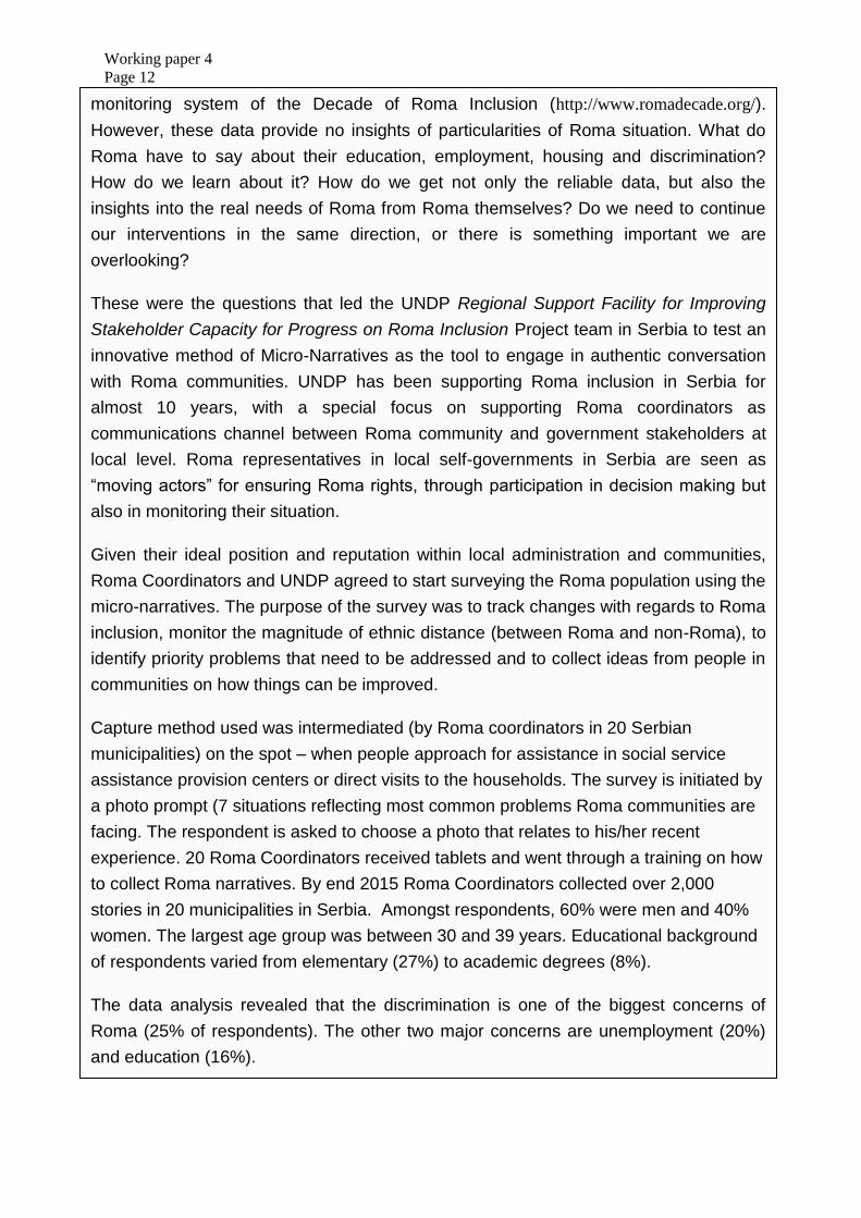
monitoring system of the Decade of Roma Inclusion (http://www.romadecade.org/).
However, these data provide no insights of particularities of Roma situation. What do
Roma have to say about their education, employment, housing and discrimination?
How do we learn about it? How do we get not only the reliable data, but also the
insights into the real needs of Roma from Roma themselves? Do we need to continue
our interventions in the same direction, or there is something important we are
overlooking?
These were the questions that led the UNDP Regional Support Facility for Improving
Stakeholder Capacity for Progress on Roma Inclusion Project team in Serbia to test an
innovative method of Micro-Narratives as the tool to engage in authentic conversation
with Roma communities. UNDP has been supporting Roma inclusion in Serbia for
almost 10 years, with a special focus on supporting Roma coordinators as
communications channel between Roma community and government stakeholders at
local level. Roma representatives in local self-governments in Serbia are seen as
“moving actors” for ensuring Roma rights, through participation in decision making but
also in monitoring their situation.
Given their ideal position and reputation within local administration and communities,
Roma Coordinators and UNDP agreed to start surveying the Roma population using the
micro-narratives. The purpose of the survey was to track changes with regards to Roma
inclusion, monitor the magnitude of ethnic distance (between Roma and non-Roma), to
identify priority problems that need to be addressed and to collect ideas from people in
communities on how things can be improved.
Capture method used was intermediated (by Roma coordinators in 20 Serbian
municipalities) on the spot – when people approach for assistance in social service
assistance provision centers or direct visits to the households. The survey is initiated by
a photo prompt (7 situations reflecting most common problems Roma communities are
facing. The respondent is asked to choose a photo that relates to his/her recent
experience. 20 Roma Coordinators received tablets and went through a training on how
to collect Roma narratives. By end 2015 Roma Coordinators collected over 2,000
stories in 20 municipalities in Serbia. Amongst respondents, 60% were men and 40%
women. The largest age group was between 30 and 39 years. Educational background
of respondents varied from elementary (27%) to academic degrees (8%).
The data analysis revealed that the discrimination is one of the biggest concerns of
Roma (25% of respondents). The other two major concerns are unemployment (20%)
and education (16%).
Working paper 4
Page 13
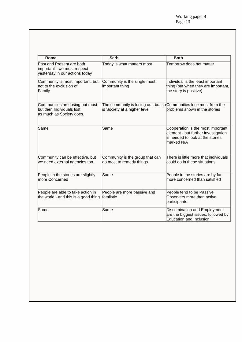
Roma Serb Both
Past and Present are both important - we must respect yesterday in our actions today
Today is what matters most Tomorrow does not matter
Community is most important, but not to the exclusion of Family
Community is the single most important thing
Individual is the least important thing (but when they are important, the story is positive)
Communities are losing out most, but then Individuals lost as much as Society does.
The community is losing out, but so is Society at a higher level
Communities lose most from the problems shown in the stories
Same Same Cooperation is the most important element - but further investigation is needed to look at the stories marked N/A
Community can be effective, but we need external agencies too.
Community is the group that can do most to remedy things
There is little more that individuals could do in these situations
People in the stories are slightly more Concerned
Same People in the stories are by far more concerned than satisfied
People are able to take action in the world - and this is a good thing
People are more passive and fatalistic
People tend to be Passive Observers more than active participants
Same Same Discrimination and Employment are the biggest issues, followed by Education and Inclusion
Working paper 4
Page 14
d. Other difficult to reach populations
In addition to the above groups, who are typically completely absent from the sampling frames of
household surveys in most countries. There are also groups who, while in theory included within the
survey population, are often very difficult to reach, leading to under-coverage in statistics. These
include fragile and disjointed households, as well as often the poorest urban populations.
There are often a variety of reasons why some sub-populations are harder to cover in surveys
including practical ones of access (e.g. accessing the individual address for those living in
flats/apartments), being present at the address when interviewers make contact, language barriers, and
unwillingness to participate in official surveys, particularly where they are collecting personal
financial information.
Working paper 4
Page 15
Section B: Welfare Measures
1. Income concepts and definitions
Drawing on the 2011 Canberra Group Handbook (UNECE, 2011), this section provides the
conceptual definition of household income, as well as details about its main component elements.
a. The income concept
The conceptual definition of household income adopted in the 2011 Canberra Group Handbook, is as
follows (ILO, 2004):
Household income consists of all receipts whether monetary or in kind (goods and services) that are
received by the household or by individual members of the household at annual or more frequent
intervals, but excludes windfall gains and other such irregular and typically one-time receipts.
Household income receipts are available for current consumption and do not reduce the net worth of
the household through a reduction of its cash, the disposal of its other financial or non-financial
assets or an increase in its liabilities.
Household income may be defined to cover: (i) income from employment (both paid and self-
employment); (ii) property income; (iii) income from the production of household services for own
consumption; and (iv) current transfers received (other than social transfers in kind); and (v) social
transfers in kind.
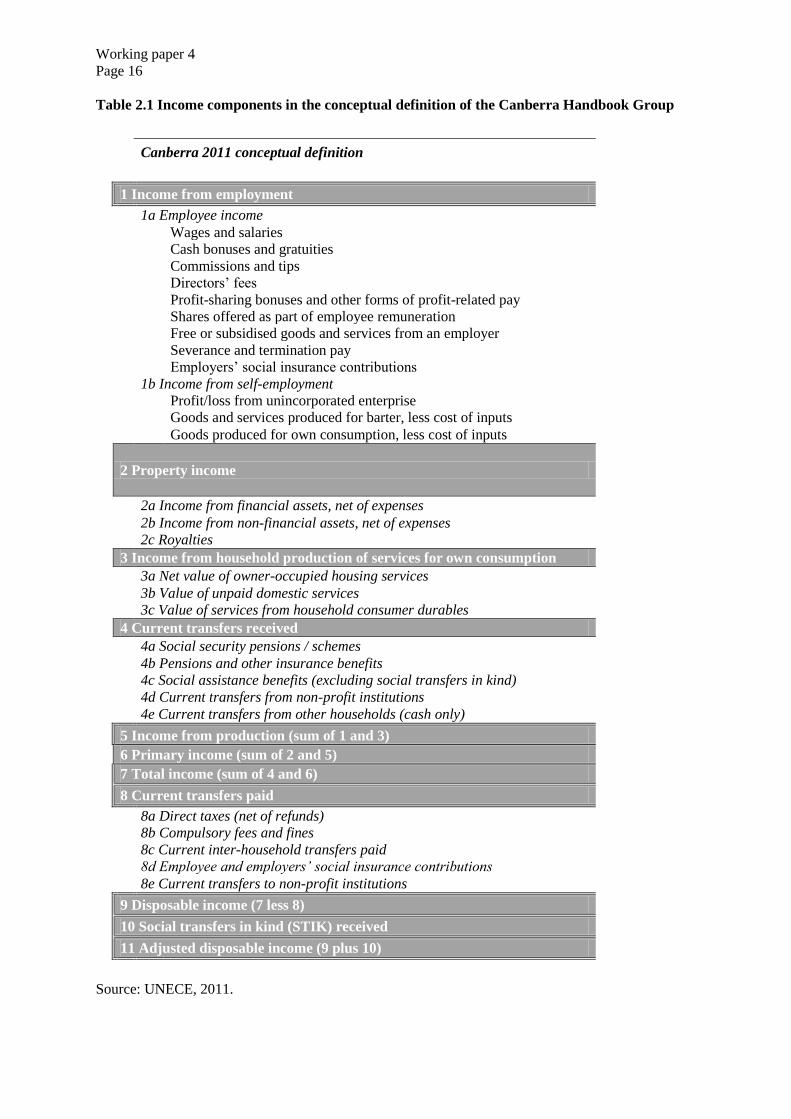
This conceptual definition determines what, in principle, should be included in a comprehensive
measure of household income (see Table 2.1). In practice, income definitions adopted by individual
countries may be more limited in scope, as some elements of household income may not be collected
or modelled (this is typically the case, for instance, of unpaid domestic services, of services from
household consumer durables, and of social transfers in kind received) .
Working paper 4
Page 16
Table 2.1 Income components in the conceptual definition of the Canberra Handbook Group
Source: UNECE, 2011.
Canberra 2011 conceptual definition
1 Income from employment
1a Employee income
Wages and salaries
Cash bonuses and gratuities
Commissions and tips
Directors’ fees
Profit-sharing bonuses and other forms of profit-related pay
Shares offered as part of employee remuneration
Free or subsidised goods and services from an employer
Severance and termination pay
Employers’ social insurance contributions
1b Income from self-employment
Profit/loss from unincorporated enterprise
Goods and services produced for barter, less cost of inputs
Goods produced for own consumption, less cost of inputs
2 Property income
2a Income from financial assets, net of expenses
2b Income from non-financial assets, net of expenses
2c Royalties
3 Income from household production of services for own consumption
3a Net value of owner-occupied housing services
3b Value of unpaid domestic services
3c Value of services from household consumer durables
4 Current transfers received
4a Social security pensions / schemes
4b Pensions and other insurance benefits
4c Social assistance benefits (excluding social transfers in kind)
4d Current transfers from non-profit institutions
4e Current transfers from other households (cash only)
5 Income from production (sum of 1 and 3)
6 Primary income (sum of 2 and 5)
7 Total income (sum of 4 and 6)
8 Current transfers paid
8a Direct taxes (net of refunds)
8b Compulsory fees and fines
8c Current inter-household transfers paid
8d Employee and employers’ social insurance contributions
8e Current transfers to non-profit institutions
9 Disposable income (7 less 8)
10 Social transfers in kind (STIK) received
11 Adjusted disposable income (9 plus 10)
Working paper 4
Page 17
b. Income components
The remainder of this section describes the component elements that constitute the conceptual
definition of household income, as defined in the 2011 Canberra Group Handbook.
Income from employment
Income from employment comprises receipts for participation in economic activities in a strictly
employment-related capacity. It consists of payments, in cash or in kind, received by individuals, for
themselves or in respect of their family members, as a result of their (current or former) involvement
in paid jobs or self-employment. Income from employment can take the form of:
Employee income received in cash (monetary) or in kind (as goods and services). Employee
income consists of direct wages and salaries for time worked and work done, commission and
piece-work payments, tips and gratuities, directors’ fees, shares offered as part of employee
remuneration, profit-sharing bonuses and other forms of profit-related pay, remuneration from
an employer for time not worked such as annual leave, holidays or other paid leave, free or
subsidised goods and services from an employer, severance and termination pay (except
lump-sum retirement payments, which are treated as capital transfers), and employers’ social
insurance contributions.
Income from self-employment, i.e. income received by individuals over a given reference
period as a result of their involvement in self-employment jobs (ILO, 2004). The basis for the
measurement of income from self-employment in household income statistics is the concept
of “net” income, i.e. the value of gross output less operating costs and after adjustment for
depreciation of assets used in production.
Property income
Property income is the flow of receipts that arise from the ownership of assets (return for use of
assets) provided to others for their use. They include returns from financial assets, from non-financial
assets and from royalties. Returns from financial assets comprise of:
Interest receipts, that is payments received from accounts with banks, building societies
and other financial institutions, government bonds and loans to non-household members.
Dividend receipts, that is payments from investment in unincorporated enterprises in
which the investor does not work (sometimes known as “sleeping” or “silent” partners),
and annuities and other regular payments from life insurance funds and private pension
funds that are excluded from social insurance.
Property income also includes:
Rents and other payments received for the use of non-financial assets, such as land, and
produced assets, such as houses, other buildings and equipment.
Royalties, i.e. receipts arising from the return for services of patented or copyright material.
Holding gains or losses, windfall gains and other such irregular and one-time receipts are excluded
from the conceptual definition of household income.
Income from the household production of services for own consumption
Income from the household production of services for own consumption includes services produced
within the household for the household’s own consumption rather than for the market. They include:
Imputed rent, that is the net estimated value of housing services from owner-occupied
dwellings. Imputed rent is included in income on a net basis, i.e. the imputed value of the
Working paper 4
Page 18
services received less the value of the housing costs incurred by the household in their role as
a landlord. While the inclusion of imputed rent in income statistics has significant merit,
cross-country comparability of estimates of imputed rent is still limited. It is therefore
recommended that where estimates of imputed rent are compiled, these should be made
separately available to support different types of analyses (ILO, 2004).
The estimated value of unpaid domestic services, such as cooking, housekeeping, minor
repairs and child care. Due to methodological limitations and data constraints that hamper
cross-country comparability, it is suggested that when the estimated value of unpaid domestic
services is compiled, this is made separately available.
The estimated value of services from household consumer durables, such as cars, washing
machines and refrigerators. Only the imputed value of the flow of services provided by these
items, less expenses incurred in providing them, is included here.
Current transfers received
Transfers are receipts for which the recipient does not give anything to the donor in direct return.
Transfers can consist of cash, of goods, or of services. Transfers may be made between households,
between households and the government, between households and corporations, or between
households and charities, both within or outside the country. They consist of all transfers that are not
transfers of capital but also exclude social transfers in kind made by governments and charities.
Current transfers tend to be small and are often made frequently and regularly. They include:
Social security pensions, insurance benefits and allowances generated from general
government-sponsored social insurance schemes (compulsory/legal schemes) such as
pensions (including overseas pensions), unemployment and sickness benefits.
Pensions and other insurance benefits, from employer-sponsored social insurance schemes
not covered by social security legislation (both funded and unfunded).
Social assistance benefits in cash from governments (universal or means-tested) that provide
the same benefits as social security schemes, but which are not provided for under such
schemes.
Current transfers from other households, in the form of family support payments (such as
alimony, child and parental support), regular receipts from inheritances and trust funds,
regular gifts, financial support or transfers in kind of goods or services (e.g. housing or child
care services), and any other cash payments or provision of goods and services intended to
support the current consumption of the recipient.
Current cash transfers from non-profit institutions (e.g. charities, trade unions and religious
bodies) in the form of gifts and financial support, such as scholarships, union strike pay,
union sickness benefits and relief payments.
Other current transfers received include current transfers from corporate entities (unless they
qualify as negative consumption expenditure) and from inheritances and trust funds.
Capital transfers received, that is transfers arising from the acquisition of assets without payment by
the receiver, are excluded from the conceptual definition of income.
Box 2.2 provides an example of statistics from Germany, who consider the number of persons
dependent on such social transfers in addition to the standard at-risk-of-poverty rate from EU-SILC.
Current transfers paid
This category includes payments such as direct taxes (net of refunds), compulsory fees or fines paid,
employer and employee contributions to social insurance schemes, current transfers to non-profit
organisations, and current transfers to other households, such as child support or alimony payments.
When considering transfers between households, it is important that statistics include both transfers in
Working paper 4
Page 19
and out of households to ensure the net position is shown (though obviously, where the data are from
surveys it is extremely unlikely that both sides of the same transaction will be shown).
Social transfers in kind
Social transfers in kind (STIK) are defined as goods and services provided by government and non-
profit institutions that benefit individuals but are provided free or at subsidised prices, e.g. food,
housing, education and health care.
c. Income aggregation
The component elements of income can be aggregated as to produce selected measures for particular
analytical and policy purposes. The sum of income from employment (1 in Table 2.1) and income
from household production of services for own consumption (3) is referred to as income from
production. Adding income from production to property income (2) gives primary income. Total
income is the sum of primary income and current transfers received (4); from this measure it is
possible to obtain disposable income, which is total income less current transfers paid (8). Total and
disposable income are the most used income aggregates.
Box 2.2 Persons at risk of poverty and beneficiaries of social transfers: Different concepts - different people? A case-study for Germany 2014
The German system of social reporting in official statistics (“amtliche Sozialberichterstattung”) provides a wide
range of comparable data on national and regional (“Länder”) level. One data source is taking stock of the
beneficiaries of the social security system. Another source is providing data on relative poverty (at–risk-of-poverty
rate). Data drawing on both sources is published online.
The national poverty rate is provided by Eurostat for all its member states based on the European household survey
EU-SILC (statistics on income and living conditions). SILC covers aspects of living conditions for households and
individuals in both monetary and non-monetary terms. Within its AROPE-concept (people at risk of poverty or social
exclusion), SILC identifies those who are in at least one of the following situations: being at risk of poverty after
social transfers; being severely materially deprived; living in households with very low work intensity. AROPE-
indicators are for example used to monitor the European 2020-strategy.
For further analyses on sub-national level, SILC has its limits with respect to the sample size which is currently
0,03% of the German population. Therefore, the risk of poverty rate on NUTS 1 (“Länder”) and NUTS 2 level (plus
additional regional breakdowns) is not based on SILC but on the “Mikrozensus”, a yearly household survey (1-%-
sample of total population). The at-risk-of-poverty rate only reflects the current income while situational needs,
wealth status and actual housing costs are not considered.
In contrast to the at-risk-of-poverty rate, the number of persons depending on social transfers is a different concept
describing people depending on public assistance in order to secure a livelihood. In Germany, the most claimed social
assistance of that type is the so called unemployment benefit II (based on Book II of the Social Code, known as the
“Hartz IV” Act). All people who are able to work, but unemployed and in need (and who are not entitled to
unemployment insurance under Social Code III) receive transfers for themselves and – if applicable – their
dependents. This includes assistance for cost of accommodation as well as mandatory health insurance. Similar
transfers are provided for persons unable to work and persons at retirement age in accordance with Social Code XII.
Data on social transfers is usually administrative data and is available for different types of social status as well as on
various regional levels. In contrast to the household survey Mikrozensus, administrative data is available on NUTS 3
(“Kreise”) level and beyond. Therefore administrative data is the main source of studies on inequality and poverty in
particular on municipal level.
Although both indicators - the poverty rate and the number of recipients of public transfers – are derived from
Working paper 4
Page 20
different data sources, are based on different definitions of poverty and are available at different regional levels, they
are both widely accepted and used in various studies on social development. Often they both complement one
another. However, they also may lead to different results and conclusions about who is at risk of poverty.
While using those two concepts, some interesting questions may arise, as for example: Is it possible for a person to
be considered poor with one definition, but not the other at the same time? The Mikrozensus is able to apply both
concepts simultaneously to the same person. For the year 2014, the main results are as follows:
17,9% (or 14,2 million) of the population in private households either live below the at-risk-of -poverty threshold
and/or do receive social transfers. This part of the population can be considered potentially poor persons. To one
third of them (32,6%) both situations applied which means their income-status keeps them below the at-risk-of-
poverty threshold while they receive social transfers at the same time. Or in other words, although they receive
transfers in order to combat poverty, they have still to be considered at risk.
More than half of the potentially poor persons (53,4%) was at risk of poverty in monetary terms, while not receiving
social transfers. One explanation may be that – although those people have to be considered as poor with regard to
their current income – they do not fulfill the conditions to receive social assistance (for example because of their
wealth status or low costs of housing/rent). Another explanation is that a large number of persons fulfills the
conditions to receive social assistance but for some reasons they do not report to social security authorities (for
example: lack of information, fear of becoming stigmatized).
Finally, 14,0% of the potentially poor persons were receiving transfers but were not at risk. With respect to income
measures after transfers, they gain an income above the poverty rate. The amount of transfers is sufficient to keep
them above at-risk-of-poverty threshold. This is the case if transfers for cost of accommodation and heating are
exceptionally high. Additional earnings and allowances to meet additional requirements of household members can
push income through transfer payments above the level of poverty risk.
Working paper 4
Page 21
2. Pros and cons of income as a welfare measure
There is no simple answer to the question of whether income or another welfare measure is preferable
for measuring monetary poverty. In practice, the decision will likely be influenced by both conceptual
and pragmatic issues. Some of the main pros and cons relating to the use of income are set out below.
a. Pros
Income measures households’ command over resources. From a conceptual perspective, income
allows people to satisfy their needs and pursue many other goals that they deem important to their
lives. In particular, a measure such as disposable income is desirable as a welfare measure as, in
general, it is an effective proxy for the resources that are available to an individual or household for
either consumption (if they so wish) or saving.
Direct policy link. Income based poverty measures are often appealing to policy makers due to the
direct policy levers that exist through, for example, targeting of social protection payments to those
families below the poverty line.
Able to break down by component. In general, it is possible to break down income by source (such
as wages, pensions, social protection receipts, intra-household transfers, etc.) when analysing poverty.
This provides both advantages in terms of understanding poverty within a certain group, and also as a
quality check for the data, through the potential to make comparisons with other sources.
Cost effective to measure. In general, data on household income is relatively cost-effective to
collect, compared with consumption expenditure. Even if no administrative data is available, the
relatively small number of potential sources of income mean that data collection is potentially more
straightforward. This makes it particularly useful where either the cost of collecting consumption data
would be prohibitive, or where precision at either the national or regional level (through a larger
sample size) is a priority.
b. Cons
The link between income and living standards not always clear. Income is a measure of potential
rather than achieved living standards. As a result, current income may either overstate the level of
living (when the family is saving, as not all the income translates into current consumption) or
understate it (when current consumption is not constrained by income, through dissaving or
borrowing) (Atkinson, 1991).
Affected by short-term fluctuations for some groups. Linked to the above point, incomes for some
population groups are particularly susceptible to short-term fluctuations, which are typically not
reflected in achieved living standards. These groups include the self-employed, agricultural workers
and those who are temporarily unemployed.
Some components are difficult to measure. Whilst data on some income components such as wages
and salaries are relatively straightforward to collect, other components including self-employment
(including agricultural work) are considerably harder to obtain accurate measures for, largely because
of the difficulty in separating out business costs and revenue. In developing countries, income data
may be particularly difficult to collect, and data accuracy is difficult to verify because most of the
population may be employed in the informal sector. There is evidence of increasing imputation rates
(due to refusal or inability to reveal specific income components) over time, in recent years (see
Meyer et al., 2015).
Evidence of under-reporting. Evidence from a range of countries suggests a general tendency for
income to be under- reported by households with low levels of resources (e.g. Meyer and Sullivan,
2011; Brewer and O’Dea, 2012). There are a number of reasons why income tends to be understated.
Working paper 4
Page 22
In part, people may forget income they have received during the reference period from sources such
as intra-household transfers, social transfers or income from items they have sold. Second, people
may be reluctant to disclose the full extent of their income, partly for privacy reasons and particularly
if any of that income has either not been disclosed to the tax authorities or has been obtained through
illegal activities (e.g. Deaton & Grosh, 2000).
3. Data Sources for Household Income
In most countries, household income microdata primarily come from household surveys developed
specifically for that purpose. However, in a number of countries (for example, the Nordic countries),
household registers are the main source of information on the distribution of household income.
Increasingly many countries are moving towards a hybrid approach, taking information on some
components of income from administrative sources (such as tax records or benefits data), and
matching that data on to survey records containing information not available from registers.
Data on household incomes are also available from National Accounts. However, the sources used for
National Accounts production typically mean that they are only available as aggregates and per capita
measures, with no distributional information available, meaning that they are of very limited use in
measuring poverty.
The collection of income data is covered in more detail in the Canberra Handbook (UNECE, 2011).
However, a summary of the main points is provided below.
a. Income surveys
Income data are usually collected through sample surveys, either from specially designed household
income surveys or from multi-topic surveys where income data are collected along with data on, for
example, household consumption or labour-force participation.
The design of the sample and the selection of sample households should be made following
appropriate sampling techniques in order to obtain results that are as precise and as accurate as
possible, within the resources that are available. The sampling method used should also permit the
calculation of sampling errors. In practice, often the sampling frame for such surveys covers only
private households, excluding institutional households and other groups (see Section A.5).
Additionally, resource limitations may mean in practice it is not possible for the sample to cover
remote regions of the country, depending on the data collection method used.
The data collection mode used for surveys collecting income data varies across countries. Probably
the most commonly used approach is face-to-face interviewing, with an interviewer visiting the
household in person. Although expensive in terms of data collection costs, face-to-face interviewing is
particularly appropriate for income surveys due to generally higher response rates and the ability of
respondents to easily refer to relevant statements or documents concerning the income questions, e.g.
their pay slip or tax return.
In some cases, face-to-face interviews are carried out using Pen and Paper Interviewing (or PAPI), in
which the interviewer records responses on a paper questionnaire. However, increasingly common,
particularly in Europe, is the use of Computer Assisted Personal Interviewing (or CAPI), in which the
interviewer asks questions from and enters data directly into a laptop or tablet.
CAPI brings with it a number of advantages which can improve the quality of income data collected.
First, as it guides the interviewer through the questionnaire, it allows for more complex routing
dependent on respondents’ previous answers than is possible with a paper questionnaire. Second, it is
possible to build checks into the questionnaire to ensure the completeness and consistency of
responses being provided. These can either be ‘hard checks’, which prevent the interviewer from
proceeding until a valid response has been provided, or ‘soft checks’, which just provide a warning
and may invite the interviewer to enter an explanation for an unusual value.
Some countries use telephone interviews to collect income data, though this is most common in
countries where it is possible to supplement survey information with administrative sources, due to
Working paper 4
Page 23
the complexities involved in collecting comprehensive income data, which requires a relatively long
interview. The detail required to collect accurate income data similarly means that other modes of
collection, such as web interviewing or postal surveys are extremely rare in this area. Income data
should ideally be collected directly from each relevant household member and separately for each
income component. Although proxy interviewing sometimes may be necessary to obtain income data
for absent household members, the quality of such data are considered inferior to data collected from
the individual household members themselves.
Household surveys are constrained by the information that respondents are able to provide with
reasonable accuracy during the course of an interview. This means that people must have knowledge
of the income they are being asked to report and must be able to recall the information with a
reasonable degree of accuracy, which may influence the accounting period used as well as the
questions asked. The questions also must appear relevant to the respondent.
A further issue with income data from social surveys, is that of decreasing response rates over time, a
phenomena seen in almost all countries, reflecting an increasing unwillingness to participate in survey
research. These falling levels of response increase the risk of non-response bias in the data.
b. Income data from registers
For countries where suitable administrative data exists, and where there is a legal basis to use them for
statistical purposes, income data from registers may be used to substitute for survey data. Nearly a
third of all countries participating in the European Union’s Statistics on Income and Living
Conditions (EU-SILC) collect at least some of their income data from registers. Outside Europe,
Canada also collects some income data from registers.
Register-based statistics can potentially provide total or near-total population coverage and can be
used to produce more detailed statistics for small areas or population groups. They can also produce
statistics for longitudinal analyses. Also, when changes occur in policy or practice, especially when
those changes affect only certain populations or geographic areas, administrative data often enable the
use of experimental or quasi-experimental research methods. Register data result in lower respondent
burden and are generally a less costly means of producing statistics, with fewer resources needed to
collect, impute or edit the collected data.
Compared to income data collected in surveys, register data are not subject to sampling and non-
response errors. They may, however, suffer from under-coverage or missing data, e.g. due to tax
evasion or low compliance. They may also be limited by the definitions and administrative practice of
the authorities responsible for the register, which may change over time.
The use of register data alongside survey data may improve the quality of income estimates that are
often underreported in household surveys and also reduce interview times and respondent burden,
which in turn opens up opportunities for alternate modes of data collection including telephone and
web-based interviewing. However, one has to be careful when carrying out this kind of exercise, as
there are some sources of non-comparability between survey and administrative data. For instance,
often the reference period for the administrative data (typically a fiscal year) does not perfectly align
with that for the survey data. Another challenge is that administrative for transfer incomes are based
on awardees, while the survey data typically provide information on the person to whom the transfer
is paid, and awardees and payees may be different people.
However, compilers of income data should be aware of some of the shortcomings of such data. In
some countries administrative data on income may be incomplete and may be available only for
people who are paying income taxes, which may exclude a significant proportion of the population. In
addition, such data will not include income earned from informal work or private income support
from other households, which in some countries may be substantial. Also, administrative data often
offer only a limited set of characteristics of individuals, and these variables are often of low quality if
not needed for program administration or other purposes.
Working paper 4
Page 24
Box 2.3 provides an example of the combined use of survey and administrative data in Italy.
Box 2.3 The combined use of survey and administrative data: a case-study for Italy
Recently, at the European level many Member States are considering an increased use of administrative
data for statistical purposes. It is driven mainly by the need to reduce the cost of data collection, to reduce
the burden on respondents, and more generally to collect data only once and use them for multiple
purposes afterwards. The main administrative sources for social statistics are population registers, tax
registers, social security data, and health and education records.
Two quality dimensions should be carefully looked at when considering a move towards an increased use
of registers, namely those of timeliness and comparability. In particular, using registers can cause
timeliness problems due to late data delivery by data owners and due to extensive practices intended to
ensure internal consistency.
The Italian SILC (It-Silc) has developed a multi-source data collection strategy in the measurement of
main income components since 2004 (Consolini, Donatiello, 2013). This strategy consists in bringing
together survey data with administrative records, by selecting an individual matching-key able to link the
same unit among different data-sources (exact record linkage). The aim of combining administrative and
survey data is to improve data quality on income components (target variables) and relative earners by
means of imputation of item non-responses and reduction of measurement errors. In addition, matching tax
returns records with survey data also provide information at micro level on social security contributions,
taxable incomes and tax liabilities. All this information is used also to measure the gross/net taxable
income by micro-simulation model.
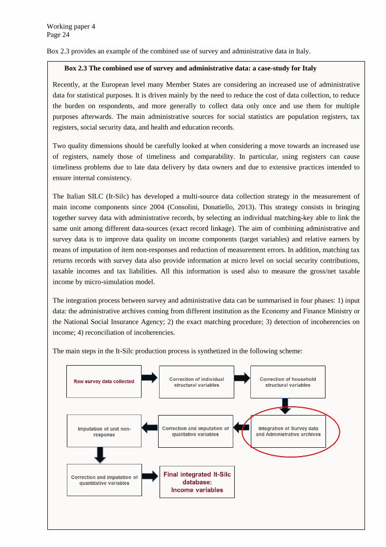
The integration process between survey and administrative data can be summarised in four phases: 1) input
data: the administrative archives coming from different institution as the Economy and Finance Ministry or
the National Social Insurance Agency; 2) the exact matching procedure; 3) detection of incoherencies on
income; 4) reconciliation of incoherencies.
The main steps in the It-Silc production process is synthetized in the following scheme:
Working paper 4
Page 25
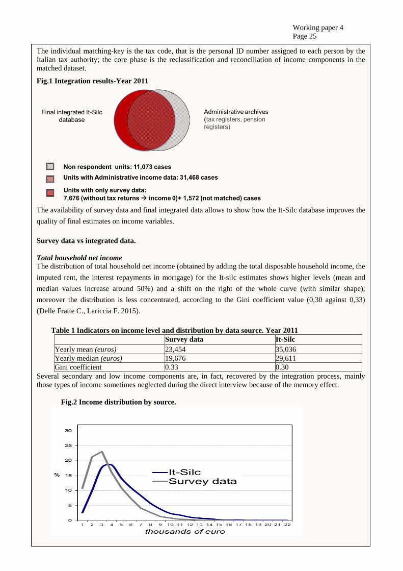
The individual matching-key is the tax code, that is the personal ID number assigned to each person by the
Italian tax authority; the core phase is the reclassification and reconciliation of income components in the
matched dataset.
Fig.1 Integration results-Year 2011
The availability of survey data and final integrated data allows to show how the It-Silc database improves the
quality of final estimates on income variables.
Survey data vs integrated data.
Total household net income
The distribution of total household net income (obtained by adding the total disposable household income, the
imputed rent, the interest repayments in mortgage) for the It-silc estimates shows higher levels (mean and
median values increase around 50%) and a shift on the right of the whole curve (with similar shape);
moreover the distribution is less concentrated, according to the Gini coefficient value (0,30 against 0,33)
(Delle Fratte C., Lariccia F. 2015).
Table 1 Indicators on income level and distribution by data source. Year 2011
Survey data It-Silc
Yearly mean (euros) 23,454 35,036
Yearly median (euros) 19,676 29,611
Gini coefficient 0.33 0.30
Several secondary and low income components are, in fact, recovered by the integration process, mainly
those types of income sometimes neglected during the direct interview because of the memory effect.
Fig.2 Income distribution by source.
Working paper 4
Page 26
The majority of changes imply an increase of income: 8.3% of the households belonging to the first and
second quintiles on the survey data, according to the It-silc data are located in the top ones (the fourth and
fifth quintiles); on the other hand, just 1.6% of the households passes from the highest to the lowest
quintile.
At-risk-of-poverty rate
Considering the at risk of poverty indicator, the value for the total population is 21.2% using survey data
and 19.6% if using It-silc. Among all, 87% of people is classified in the same way by survey and in It-silc
data.
Table 2. People at risk of poverty by data source. Year 2011 (percentage values)
Survey data It-Silc % composition
At risk of poverty At risk of poverty 13.8
At risk of poverty Not at risk of poverty 7.4
Not at risk of poverty At risk of poverty 5.8
Not at risk of poverty Not at risk of poverty 73.0
Total 100.0
The severe deprivation index1 (independent on income) was calculated for both sub-populations: among
the people classified as at risk of poverty in the survey data but not in It-silc data, the severe deprivation
index value is lower (21.9%) than the value obtained among the at risk of poverty people in both data
(31.1%).
Integrated data vs. administrative data.
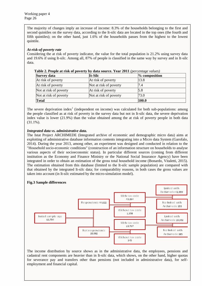
The Istat Project ARCHIMEDE (Integrated archive of economic and demographic micro data) aims at
exploiting of administrative database information contents integrating into a Micro data System (Garofalo,
2014). During the year 2013, among other, an experiment was designed and conducted in relation to the
"Household socio-economic conditions" (construction of an information structure on households to analyse
various aspects of their socioeconomic status). In particular different sources (coming from different
institution as the Economy and Finance Ministry or the National Social Insurance Agency) have been
integrated in order to obtain an estimation of the gross total household income (Bonardo, Vitaletti, 2015).
The estimation obtained from this database (limited to the It-silc sample population) are compared with
that obtained by the integrated It-silc data; for comparability reasons, in both cases the gross values are
taken into account (in It-silc estimated by the micro-simulation model).
Fig.3 Sample differences
The income distribution by source shows as in the administrative data, the employees, pensions and
cadastral rent components are heavier than in It-silc data, which shows, on the other hand, higher quotas
for severance pay and transfers other than pensions (not included in administrative data), for self-
employment and financial capital.
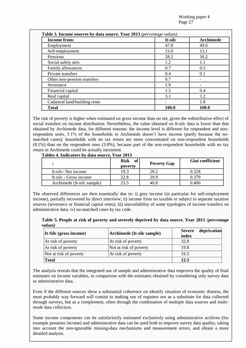
Working paper 4
Page 27
Table 3. Income sources by data source. Year 2013 (percentage values)
Income from: It-silc Archimede
Employment 47.8 49.6
Self-employment 15.0 13.1
Pensions 28.2 30.2
Social safety nets 1.2 1.1
Family allowances 0.7 0.5
Private transfers 0.4 0.1
Other non-pension transfers 0.7 -
Severance 1.9 -
Financial capital 1.5 0.4
Real capital 3.1 3.2
Cadastral land/building rents - 1.8
Total 100.0 100.0
The risk of poverty is higher when estimated on gross income than on net, given the redistributive effect of
social transfers on income distribution. Nevertheless, the value obtained on It-silc data is lower than that
obtained by Archimede data, for different reasons: the income level is different for respondent and non-
respondent units, 5.1% of the households in Archimede doesn’t have income (partly because the no-
matched cases); households with no tax return are more concentrated on non-respondent households
(8.1%) than on the respondent ones (3.8%), because part of the non-respondent households with no tax
return in Archimede could be actually inexistent.
Tables 4. Indicators by data source, Year 2013
: Risk of
poverty Poverty Gap
Gini coefficient
It-silc- Net income 19.3 28.2 0.328
It-silc - Gross income 22.8 29.9 0.379
Archimede (It-silc sample) 25.5 40.8 0.400
The observed differences are then essentially due to: i) grey income (in particular for self-employment
income), partially recovered by direct interview; ii) income from no taxable or subject to separate taxation
sources (severance or financial capital rents); iii) unavailability of some typologies of income transfers on
administrative data; iv) no-matched cases by tax code.
Table 5. People at risk of poverty and severely deprived by data source. Year 2011 (percentage
values)
It-Silc (gross income) Archimede (It-silc sample) Severe deprivation
index
At risk of poverty At risk of poverty 32.8
At risk of poverty Not at risk of poverty 19.8
Not at risk of poverty At risk of poverty 16.5
Total 12.3
The analysis reveals that the integrated use of sample and administrative data improves the quality of final
estimates on income variables, in comparison with the estimates obtained by considering only survey data
or administrative data.
Even if the different sources show a substantial coherence on identify situation of economic distress, the
most probably way forward will consist in making use of registers not as a substitute for data collected
through surveys, but as a complement, often through the combination of multiple data sources and multi-
mode data collection.
Some income components can be satisfactorily estimated exclusively using administrative archives (for
example pensions income) and administrative data can be used both to improve survey data quality, taking
into account the non-ignorable missing-data mechanisms and measurement errors, and obtain a more
detailed analysis.
Working paper 4
Page 28
The choice is a trade-off between higher accuracy and coverage rate on the target population and the
reduction of timeliness (due to temporal constraint related to the acquisition timing of administrative data
and to the ‘heavier’ process to combine Survey data and Administrative archives at micro level) and of
coherence (administrative data are collected by conforming the administrative aims and definitions, not the
statistical ones).
References
Delle Fratte C., Lariccia F. (2015) The impact of Administrative data on final estimates of It-Silc income
variables, paper presented at London EU-SILC Best Practice Workshop, 16th and 17th September 2015.
D. Bonardo, S. Vitaletti (2015), Una lettura comparative «Eu-Silc e Archimede» per l’analisi delle
condizioni socioeconomiche delle famiglie, presented at Seminario di chiusura delle attività del GdL 5
“per il supporto al Progetto Archimede”, 23 Novembre 2015.
P. Consolini, G. Donatiello (2013) Improvements of data quality through the combined use of survey
and administrative sources and micro simulation model in The use of registers in the context of EU–
SILC:challenges and opportunities, (eds. M. Jäntti, V.Törmälehto, E. Marlier), Eurostat, Statistical
working papers.
G. Garofalo (2014) Il Progetto ARCHIMEDE obiettivi e risultati sperimentali, Istat working papers n.
9/2014, Istituto Nazionale di Statistica.
Working paper 4
Page 29
4. Consumption expenditure concepts & definitions
In summarizing the main concepts and definitions, this section draws on the OECD Framework for
Statistics on the Distribution of Income, Consumption & Wealth (OECD, 2013). According to this
document, consumption expenditure represents “the value of consumption goods and services used or
paid for by a household to directly meet its needs. These goods and service are obtained:
through the purchase of goods and services in the market;
as in-kind income from employers, from self-employment (through the barter of goods and
services produced by the household), or from property or other investments (e.g. portion of
crop provided by share-farming tenant);
from the household’s own production of goods and services; or
as transfers in kind from other households or from businesses.”
If the goods and services included in consumption expenditure were produced by the person
themselves or were received from elsewhere as income in kind, the notional market value of the goods
and services is included as consumption expenditure.
Excluded from consumption expenditure are expenses not directly aimed at meeting household needs,
such as current transfers to government, social organisations or other households. These are classified
as non- consumption current expenditure. Also excluded is the payment of interest on any consumer
credit which the household may have
In measuring the consumption expenditure of households, there are a number of approaches that can
theoretically be taken to recording the expenditure. With the acquisition approach, goods and services
are included when they are acquired or taken possession of, regardless of whether they have been paid
for or, in the case of goods, regardless of whether they have been used. With the use approach, goods
and services are included when they are used, regardless of when they were acquired or paid for.
While the use approach may more closely equate to consumption, the OECD Framework recommends
use of acquisition approach for practical reasons (though in practice, for most consumption goods and
services there will be little difference between the two approaches.
The assumption does not hold for dwellings or for goods that can be used repeatedly over a length of
time, often known as consumer durables. Consumer durables include motor vehicles, electrical
appliances, furniture, clothing, and the like that would normally be expected to be usable for more
than a year. When a household purchases a dwelling or consumer durables, it does not normally
consume them immediately. Rather, the household can be viewed as a producing entity that invests in
those items as capital expenditure and provides a flow of services to itself as a consuming entity.
In the OECD Framework, it is therefore the flow of services obtained from consumer durables and
owner occupied housing that is included as consumption expenditure, rather than the initial purchase
of the capital items.
5. Pros and cons of consumption expenditure as a welfare measure
a. Pros
Better proxy of material living standards. It is the consumption of goods and services along with
other inputs such as time that ultimately satisfies a household’s needs and wants. Because of this,
consumption expenditure can be considered a more direct measure of achieved living standards than
income.
Working paper 4
Page 30
Short-term fluctuations smoothed out. households can smooth consumption by, for example,
adjusting savings or drawing on wealth and borrowing. Incomes may also be more volatile, a finding
that led to Friedman’s “permanent income hypothesis”, which suggests that decisions made by
consumers are based on long-term income expectations rather than their current income. This does not
mean that consumption is not subject to seasonal fluctuations, but these are supposedly smaller than
seasonal income fluctuations. Nevertheless, expenditures volatility may be high under some
circumstances, for example when the population makes purchases in large volumes and low
frequency, or in agricultural societies, whose incomes and expenditures are highly correlated with the
production cycles
Data quality arguably better, at least at bottom of distribution. It is often suggested that the
quality of data on consumption expenditure is better than that for income, at least towards the bottom
of the income distribution, though this depends on the collection method, as well as other factors such
as the length of reference period used. In part this potential advantage is because questions about
consumption are usually viewed as less sensitive than questions about income (though see below for
exceptions). Also, as a shorter reference period can be used (at least for day to day expenditures),
leading to less opportunity for recall errors.
b. Cons
Under-reporting of certain expenditures. Certain groups of expenditures are typically
underestimated in surveys because of under-reporting by respondents. The expenditures usually most
under-reported are those for illegal goods and services (e.g. illegal drugs and prostitution) or for
socially unacceptable goods or services (e.g. alcohol, gambling). Also, Recent evidence shows that
while reporting rates for some of the biggest components of consumption have remained stable over
time, there have been noticeable declines for some categories such as food away from home, shoes
and clothing, alcoholic beverages (see Bee, Meyer, and Sullivan, 2015).
Irregular expenditure on high value items. Whilst a diary period of a couple of weeks may, in the
majority of cases, provide a good indication of typical expenditure on categories such as food, drink
and transport, expenditure on high value items is typically infrequent, and may not be properly
reflective even when a survey with an annual reference period is used. While, at the aggregate level,
this may provide a reliable measure of household expenditure, for individual household it will lead to
‘noisy’ data with levels of total consumption expenditure not necessarily indicative of material living
standards.
Indirect policy levers. Beyond subsistence minimums, levels of consumption expenditure are largely
an issue of personal choice. As a consequence, while governments may take steps to either increase
the resources available for consumption, increase the potential to acquire those resources, or otherwise
improve the material living standards of those in poverty (by, for example, improvements to social
housing), these may not be directly reflected in the recorded consumption expenditure of households.
Data collection complex/expensive. As highlighted in the previous section, regardless of the method
used, the collection of detailed household consumption expenditure data is expensive, considerably
more so than income data. In particular, the cost of conducting Household Budget Surveys is such
that, in many European countries, they are conducted approximately once every 5 years. This makes
them unsuitable for effective poverty policy monitoring in those countries.
Individual choice. In some circumstances, low levels of consumption may in part reflect individual
choices or non-monetary constraints. For example, elderly people with physical limitations, such as
lack of mobility, may have low levels of consumption expenditure despite adequate financial
resources. Whether individual choice presents an issue for consumption expenditure based measures
depends a large extent on the level of threshold used. Where a threshold is at or close to subsistence
minimum levels, it is obviously less likely that choice will play a significant factor in consumption
expenditure around that point.
Working paper 4
Page 31
6. Data sources for consumption expenditure
a. Household Surveys
Data on consumption expenditure are collected through household surveys, either through Household
Budget Surveys explicitly focussed on expenditure (as well as possibly income), or more general
surveys covering a wider range of topics. While data on consumption expenditure for households are
available from National Accounts, again the aggregate nature of the data make them unsuitable for
poverty measurement.
Household Budget Surveys can vary widely in terms of design, however one common feature is that
almost all are primarily designed to provide expenditure weights for measures of inflation and to feed
into the production of the National Accounts. As a consequence, there is considerable focus in the
survey on detailed categories of expenditure, which limits the potential to collect information on
individual and household characteristics and other items relevant to increased understanding of
poverty within a country.
By contrast, the Living Standards Measurement Study (LSMS) surveys, first developed by the World
Bank in the 1980s, are multi-purpose household surveys as well as collecting the information
necessary to measure living standards through household consumption (though in considerably less
detail than typical Household Budget Surveys). Additional topics covered include health, education,
employment, migration and savings. As with EU-SILC in many European countries, this wider range
of data collected alongside the main welfare indicator aids the development of effective policies for
the reduction of poverty both now and in the future.
b. Retrospective vs. ongoing collection
Data on consumption expenditure are collected retrospectively and/or on an on-going basis. Data
collected retrospectively are collected by an interviewer or via a questionnaire completed by the
respondent. When conducted by an interviewer, data are collected through face-to-face interviews or
by telephone. Retrospective collection means that data are collected for an earlier time period. Data
collected on an ongoing basis are collected through the use of a diary (either paper or electronic)
completed by the household.
Both methods imply the risk of errors: omission of certain expenses (especially for small expenses
when using retrospective methods) or the inclusion of expenditures outside the reference period (when
there is telescoping of expenditures and no bounding interview).
Both retrospective interviews and diaries are big burdens for households. Retrospective interviews can
be very time-consuming when many expenditure items are being reported, for large households or for
households with complex structures. Diaries can place a large burden on respondents too, as reporting
periods can vary from several days to several months, although usually the recording period is daily
for one to two weeks.
7. Using multiple welfare measures
As highlighted above, both income and consumption expenditure have particular strengths and
weaknesses as welfare indicators for the measurement of poverty. In addition, other forms of poverty
measure covered in later chapters (such as material deprivation) have their own set of advantages (and
disadvantages) with respect to such monetary indicators.
Additionally, by looking at the intersection of multiple indicators for the same people, it is possible to
obtain new insights. Where a household is income poor but is maintaining expenditure and is not
materially deprived (those in income poverty only), this may indicate that the household is able to
draw on savings or access loans either informally or formally to maintain living standards. In some
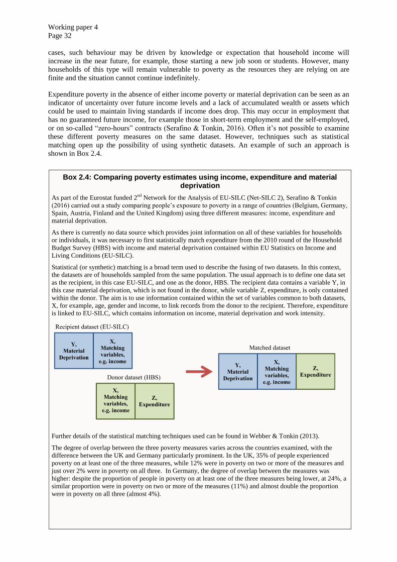
Working paper 4
Page 32
cases, such behaviour may be driven by knowledge or expectation that household income will
increase in the near future, for example, those starting a new job soon or students. However, many
households of this type will remain vulnerable to poverty as the resources they are relying on are
finite and the situation cannot continue indefinitely.
Expenditure poverty in the absence of either income poverty or material deprivation can be seen as an
indicator of uncertainty over future income levels and a lack of accumulated wealth or assets which
could be used to maintain living standards if income does drop. This may occur in employment that
has no guaranteed future income, for example those in short-term employment and the self-employed,
or on so-called “zero-hours” contracts (Serafino & Tonkin, 2016). Often it’s not possible to examine
these different poverty measures on the same dataset. However, techniques such as statistical
matching open up the possibility of using synthetic datasets. An example of such an approach is
shown in Box 2.4.
Box 2.4: Comparing poverty estimates using income, expenditure and material deprivation
As part of the Eurostat funded 2nd
Network for the Analysis of EU-SILC (Net-SILC 2), Serafino & Tonkin
(2016) carried out a study comparing people’s exposure to poverty in a range of countries (Belgium, Germany,
Spain, Austria, Finland and the United Kingdom) using three different measures: income, expenditure and
material deprivation.
As there is currently no data source which provides joint information on all of these variables for households
or individuals, it was necessary to first statistically match expenditure from the 2010 round of the Household
Budget Survey (HBS) with income and material deprivation contained within EU Statistics on Income and
Living Conditions (EU-SILC).
Statistical (or synthetic) matching is a broad term used to describe the fusing of two datasets. In this context,
the datasets are of households sampled from the same population. The usual approach is to define one data set
as the recipient, in this case EU-SILC, and one as the donor, HBS. The recipient data contains a variable Y, in
this case material deprivation, which is not found in the donor, while variable Z, expenditure, is only contained
within the donor. The aim is to use information contained within the set of variables common to both datasets,
X, for example, age, gender and income, to link records from the donor to the recipient. Therefore, expenditure
is linked to EU-SILC, which contains information on income, material deprivation and work intensity.
Further details of the statistical matching techniques used can be found in Webber & Tonkin (2013).
The degree of overlap between the three poverty measures varies across the countries examined, with the
difference between the UK and Germany particularly prominent. In the UK, 35% of people experienced
poverty on at least one of the three measures, while 12% were in poverty on two or more of the measures and
just over 2% were in poverty on all three. In Germany, the degree of overlap between the measures was
higher: despite the proportion of people in poverty on at least one of the three measures being lower, at 24%, a
similar proportion were in poverty on two or more of the measures (11%) and almost double the proportion
were in poverty on all three (almost 4%).
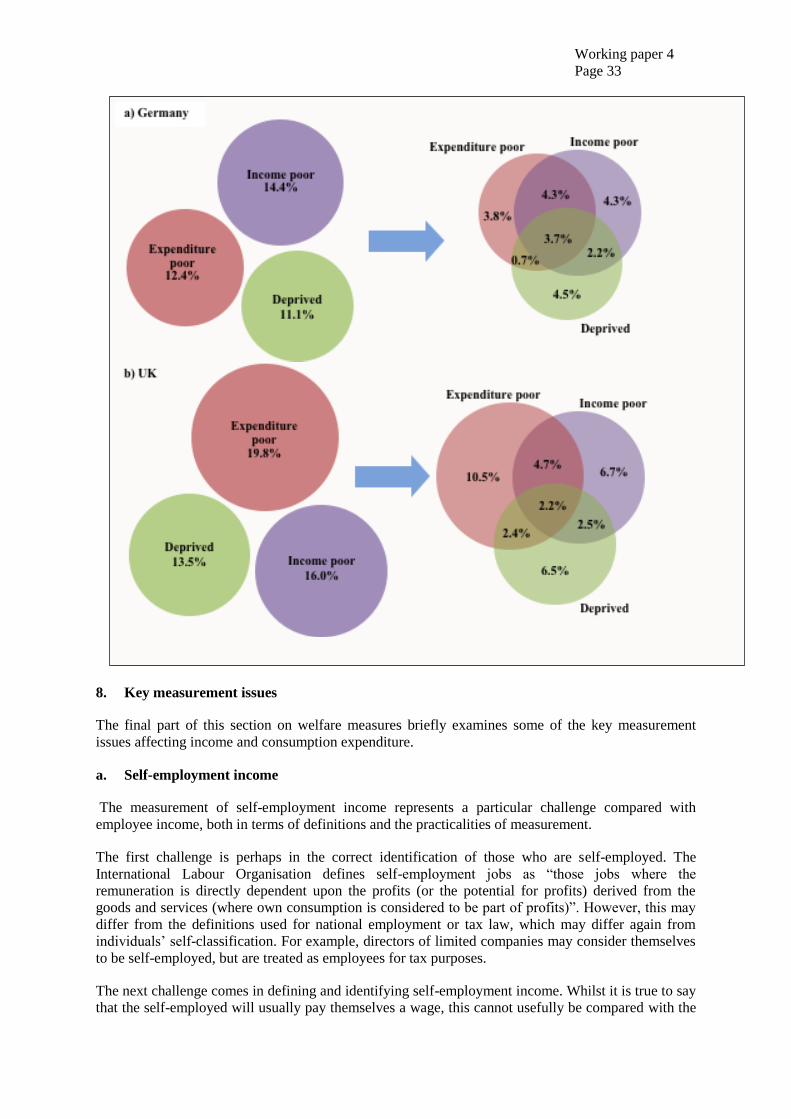
Working paper 4
Page 33
8. Key measurement issues
The final part of this section on welfare measures briefly examines some of the key measurement
issues affecting income and consumption expenditure.
a. Self-employment income
The measurement of self-employment income represents a particular challenge compared with
employee income, both in terms of definitions and the practicalities of measurement.
The first challenge is perhaps in the correct identification of those who are self-employed. The
International Labour Organisation defines self-employment jobs as “those jobs where the
remuneration is directly dependent upon the profits (or the potential for profits) derived from the
goods and services (where own consumption is considered to be part of profits)”. However, this may
differ from the definitions used for national employment or tax law, which may differ again from
individuals’ self-classification. For example, directors of limited companies may consider themselves
to be self-employed, but are treated as employees for tax purposes.
The next challenge comes in defining and identifying self-employment income. Whilst it is true to say
that the self-employed will usually pay themselves a wage, this cannot usefully be compared with the
Working paper 4
Page 34
earnings of employees. This is because self-employed workers frequently take a small salary in favour
of taking dividends or putting profits into the company.
Clear definitions in any survey questions are vital, as what individuals may think of as their income
may differ from what is considered income under the definitions used (e.g. those from the UNECE
Canberra Handbook, 2011). Additionally, there is also an issue that self-employed individuals may
not themselves be able to provide an accurate estimate of their income, particularly if they have not
yet (or are not required to) filed their end-of-year accounts with the tax authorities.
Where possible, asking about profits and other data items typically required for tax purposes is still
the preferred approach for survey data collection. Where a respondent has not prepared accounts for
the tax authorities, the alternative approach is to collect data on any earnings from their business, plus
any money that has been drawn from their business accounts for personal use.
b. Goods/services produced for own consumption
Home production for own consumption refers to the goods or services that are produced within the
household for the household’s own consumption, rather than for sale or exchange. The estimated
market value of the goods/services is included as part of households’ self-employment income, less
any expenses incurred in their production. The value of these goods and/or services should also be
counted as part of households’ consumption expenditure.
The relative contribution of goods produced for own consumption can vary considerably between
economies. In some countries, the value of such goods and the proportion of households producing
them may be negligible. Where that is the case, they are often excluded from income statistics.
However, in other economies, particularly agricultural, the value of own consumption may be
substantial for many households, in which case it is vital to capture, to ensure the economic well-
being of those households
Two particular examples of home production for own consumption are described in further detail
below: Housing services from owner-occupied dwellings, and consumer durables.
Housing Services from owner-occupied dwellings
Owning your own house or apartment in effect provides you with housing services which should be
considered as part of both income and consumption. The value of such housing services is estimated
as being the market rent for a similar property, less the costs incurred by the household in their role as
landlord. These housing services should feature in both income, increasing the level of household
resources, consumption expenditure, contributing to the household’s economic well-being. Including
net imputed rent is particularly important when making comparisons of poverty across countries,
where rates of home ownership can vary wildly.
Where there is an established rental market, the rental equivalence approach is generally considered
the preferred approach to estimating imputed rental values. The basic econometric method that is used
is hedonic regression with the attributes of the dwelling used as covariates. If there is selection bias, a
Heckman correction may be applied, with a model for the housing tenure and a model for the
imputation of the values. An alternative approach is to use cell-based mean imputation, what is
typically referred to as the stratification method.
Where rental markets are less well-developed, one commonly used alternative to rental equivalence is
the user cost method, based on the estimation of the cost incurred for homeownership by foregoing
the opportunity to invest in financial assets from which real income flows are created in the form of
income from interest and dividends. A further alternative is self-assessment, effectively asking how
much you would have to pay if, instead of owning your home, you had to rent it.
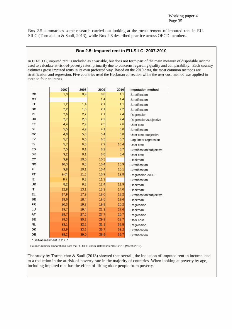
Working paper 4
Page 35
Box 2.5 summarises some research carried out looking at the measurement of imputed rent in EU-
SILC (Tormalehto & Sauli, 2013), while Box 2.8 described practice across OECD members.
Box 2.5: Imputed rent in EU-SILC: 2007-2010
In EU-SILC, imputed rent is included as a variable, but does not form part of the main measure of disposable income
used to calculate at-risk-of-poverty rates, primarily due to concerns regarding quality and comparability. Each country
estimates gross imputed rents in its own preferred way. Based on the 2010 data, the most common methods are
stratification and regression. Five countries used the Heckman correction while the user cost method was applied in
three to four countries.
The study by Tormalehto & Sauli (2013) showed that overall, the inclusion of imputed rent in income lead
to a reduction in the at-risk-of-poverty rate in the majority of countries. When looking at poverty by age,
including imputed rent has the effect of lifting older people from poverty.
14
2 Measuring imputed rents
The distributional impact of imputed rent in EU-SILC 2007-2010
(2010) and Eurostat (2009). Both the covariates used and the use of either the regression or stratification
method may have an effect on the distribution of the estimated rental equivalences. The Heckman
selection model is one way to tackle the possible selection bias induced by the segregation between
owners and tenants: the “donors” (private rental tenants) may differ substantially from the “recipients”
(owners) in many respects, such as floor area, location, or quality of housing(5)
.
Eurostat guidelines cited above set the threshold of the size of the market rent sector rather low (10%) for
choosing the user cost method. In 2007, 17-18 countries went under this threshold. In 2009, 13 countries
went under it, and four countries hardly exceeded the threshold. Three of them have adopted the user cost
method at the outset. Only one country (Cyprus, where the share of population on the rental market was
9.9 in 2007) among countries with a small market rent sector has reported of the use of Heckman
correction to tackle the possible selection bias emerging from the possible segregation between owners
and tenants.
Table 1: The share of market renters, % from population. Countries arranged by the
share of market renters in 2009.
Source: authors’ elaborations from the EU-SILC users’ databases 2007–2010 (March 2012).
NB: In Romania, share of persons in households paying market rents, was stable around one per cent of the population 2007–2010.
(5) These can be related to the discussion on dualist and unitary housing systems (Kemeny, 1996; Juntto & Reijo, 2010): to the level of segregation
between rental and owned dwelling stock, and to the level of segregation within rental markets between private and social housing.
2007 2008 2009 2010 Imputation method
RO 1,0 0,9 0,8 1,1 Stratification MT 1,4 1,4 Stratification LT 1,2 1,4 2,1 1,1 Stratification BG 2,2 1,6 2,1 2,2 Stratification PL 2,6 2,2 2,1 2,4 Regression HU 2,7 2,6 2,2 2,4 Regression/subjective EE 4,4 2,9 2,5 2,6 User cost SI 5,5 4,9 4,1 5,0 Stratification CZ 4,8 5,0 5,4 5,0 User cost, subjective LV 5,7 6,6 6,3 6,7 Log-linear regression IS 5,7 6,8 7,9 10,4 User cost ES 7,5 8,1 8,2 8,7 Stratification/subjective SK 9,2 9,1 8,8 8,4 User cost CY 9,9 10,6 10,3 Heckman NO 10,3 9,8 10,4 10,9 Stratification FI 9,8 10,1 10,4 10,1 Stratification PT 9,6* 11,3 10,9 12,8 Regression 2008- IE 8.7 9,3 11,3 Stratification UK 8,2 9,3 12,4 11,9 Heckman IT 12,8 13,1 13,3 14,0 Heckman EL 17,9 17,9 18,0 18,2 Stratification/subjective BE 18,6 18,4 18,5 19,6 Heckman FR 20,3 19,3 19,8 20,2 Regression LU 19,7 19,4 22,3 27,6 Heckman AT 28,7 27,5 27,7 26,7 Regression SE 28,3 30,2 29,8 28,7 User cost NL 33,1 32,2 31,1 32,5 Regression DK 32,9 33,5 33,7 33,2 Stratification DE 38,2 39,0 38,9 39,7 Stratification
* Self-assessment in 2007
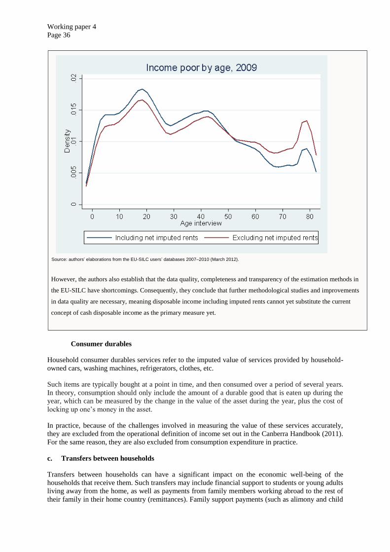
Working paper 4
Page 36
Consumer durables
Household consumer durables services refer to the imputed value of services provided by household-
owned cars, washing machines, refrigerators, clothes, etc.
Such items are typically bought at a point in time, and then consumed over a period of several years.
In theory, consumption should only include the amount of a durable good that is eaten up during the
year, which can be measured by the change in the value of the asset during the year, plus the cost of
locking up one’s money in the asset.
In practice, because of the challenges involved in measuring the value of these services accurately,
they are excluded from the operational definition of income set out in the Canberra Handbook (2011).
For the same reason, they are also excluded from consumption expenditure in practice.
c. Transfers between households
Transfers between households can have a significant impact on the economic well-being of the
households that receive them. Such transfers may include financial support to students or young adults
living away from the home, as well as payments from family members working abroad to the rest of
their family in their home country (remittances). Family support payments (such as alimony and child
However, the authors also establish that the data quality, completeness and transparency of the estimation methods in
the EU-SILC have shortcomings. Consequently, they conclude that further methodological studies and improvements
in data quality are necessary, meaning disposable income including imputed rents cannot yet substitute the current
concept of cash disposable income as the primary measure yet.
33
5 Changes in income poverty
The distributional impact of imputed rent in EU-SILC 2007-2010
5. Changes in income poverty
Given the sizable level and distributional effects, the addition of imputed rents may also change the time
series of key indicators. As already shown, the supranational indicators of income inequality do not point
to different trends in time. We next compare the trend of income poverty with and without imputed rents
at country level.
The general net effect of re-ranking households and individuals on the income scale caused a decrease in
general at-risk-of-poverty rates in the majority of countries in the 2007 data (Törmälehto and Sauli 2010).
This was an outcome of a) increase in median income and consequently in income poverty threshold
(decrease in NL and NO), b) transitions out of poverty (“cash poor”) and c) transitions into poverty
(“house poor”).
As a reminder of the general impact of imputed rents on poverty, Figure 10 shows the supranational age
distribution of poor individuals with and without net imputed rents. As expected, imputed rents lift older
people from income poverty while the new entries are mostly younger, with exits surpassing entries
roughly from 50 years upwards. This reflects the life-cycle properties of homeownership rates and
mortgage indebtedness.
Figure 10: Age distribution of the income poor with and without imputed rents, 2009.
Supranational kernel density estimates (all countries except DE, MT, BG, CY, IE).
Source: authors’ elaborations from the EU-SILC users’ databases 2007–2010 (March 2012).
To get an overview of the stability of the transitions over the years, we computed age distributions of
those who enter or exit poverty when net imputed rents are added. As shown in Figure 11, the age profiles
have some variation across the years, but overall shapes are reasonably similar. The older age groups, and
particularly those above 70+, exit poverty while the entries come broadly from younger age groups up to
around 40 years.
Working paper 4
Page 37
and parental support) also fall into this category.
The OECD Framework for Income, Consumption & Wealth statistics (2013) indicates that Inter-
household transfers are:
Given without an expectation of repayment, similar to any current transfer.
Given with the aim of supporting current consumption; this is related to the classification of a
specific economic flow between households as income received (when money, goods or
services are used immediately or in the short-term) or as an increment of wealth (when saved
or comprising a capital item such as a consumer durable).
Often made regularly, i.e. anticipated or relied upon by the recipient household. . Regular
inter-household transfers include regular alimonies, child and parental support payments,
either voluntary or compulsory. Inter-household transfers can be donated either by family
members or by any other person not living in the recipient household.
. While regular inter-household transfers are included as income, any transfers in kind (such as food)
are additionally be counted as part of consumption expenditure by the recipient household.
. If the transfer between households is of a consumer durable or asset, intended to support the
purchase of an asset, or it is expected that the majority of the value will be used for saving (or paying
off debt), the transfer is not considered income, but rather a capital transfer.
Working paper 4
Page 38
Box 2.6 provides an example of the impact of remittances on poverty in the Europe and Central Asia
Region.
d. Social Transfers in Kind
The Canberra Group Handbook (2011) defines social transfers in kind (STIK) as goods and services
provided by government and non-profit institutions that benefit individuals but are provided free or at
subsidised prices. The Handbook recommends that where possible, it is desirable to add the value of
Box 2.6 Remittances and poverty
Europe and Central Asia region show high rates of mobility, which developed in a number of waves during last
decades after the fall of Berlin wall and Iron curtain. First waves of migration were associated with return of
people to their newly independent nation states, as well as waves of refuges and internally displaced people fleeing
from violent conflicts (especially at Western Balkans). More recent waves of migrants are in larger extend driven
by economic considerations—lack of productive employment at home and better possibilities abroad. Migration
patterns are shaped by complex interplay of cultural, linguistic, economic and political factors. Labour migration
and associated remittances became huge in the region—three out of top-5 countries by remittances to GDP ratio
are Tajikistan, Kyrgyzstan and Moldova. Armenia, Kosovo*, Georgia and Bosnia and Herzegovina enjoy
remittances-to-GDP ratio higher than 10%. For lower income countries of region remittances are coming close to
export receipts and dwarf FDI and ODA flows. Not surprise remittances deeply affect whole countries and
individual families.
Countries try to track poverty reduction effect of remittances, collecting data through Household budget surveys.
Kyrgyzstan National Statistical Committee regularly reports poverty rates with and without remittances, including
breakdown by regions. Data show profound impact of remittances, reducing poverty from 36.4 to 30.6 percent.
This impact is more pronounced for extreme poverty (which goes down from 7.7 to 1.2 percent) and for less
developed southern regions, like Jalal-Abad, Batken, Osh and city Osh. In Moldova National Bureau of Statistics
supplies data to Ministry of Economy and Trade, which is responsible for poverty monitoring. NBS publishes only
structure of incomes, which includes remittances. Ministry of Economy publishes poverty data with and without
transfers in its annual poverty monitoring reports. In 2014 remittances reduced poverty rates by some 15pp, from
26.7 to 11.4 percent. Moldova HBS is not representative by territorial units, as rayons in Moldova are much
smaller than oblast in Kyrgyzstan, however provides data for urban and rural areas. Remittances play bigger role
for villages, reducing poverty from 35.3 to 16.4 percent. In Armenia National Statistical Service publishes share of
remittances in household incomes (which on average was as high as 10.4 percent in 2014), but do not report
poverty rates without remittances. Ukraine Statistical Office reports share of a broad category “Money transfers
from relatives and other persons; other cash incomes” (7 percent in 2014).
There are some methodological issues around these figures. Respondents could be reluctant to report remittances
from abroad (however, massive migration and widespread of remittances could reduce this concern, as people get
habitual to it). Remittances could come irregularly and not fall into reporting timeframe of HBS. Migration could
affect whole household, which thus will not be included in Survey. IMF study at household level data for Armenia
finds systematic under-reporting of remittances and estimated share of underreporting at some 30%. Last but not
the least, poverty reduction effect of remittances should be treated with caution, as it doesn’t take into account
some other effects caused by migration. On the one hand, it doesn’t take into account opportunity costs—back at
home migrants would find some jobs, lower paid than abroad, but nevertheless bringing some money. On the other
hand, remittances reduce labour supply of households, consequently reducing incomes of families.
Working paper 4
Page 39
social transfers in kind to household disposable income to create a measure of adjusted disposable
income. Similarly, social transfers in kind added to consumption expenditure provides a measure of
Actual final consumption. This is the total value of all goods and services used by the household to
meet the needs of its members.
Taking into account STIK is particularly important when the purpose of analysis is to make cross-
country comparisons of poverty. This is because in one country (A), certain services may be largely
provided by the state, free at the point of use, whereas in Country B it may be necessary to pay for
those services directly. This means that, all other factors being equal, someone with the same
disposable income (or consumption expenditure) in Country A would have a higher standard of living
than in Country B.
Social transfers in kind are also very important for measuring economic well-being within countries.
Since one of the major policy aims in this area is often to make access to important services more
equal, the distribution of STIK is generally progressive. Additionally, over time, both the level and
form of STIK are likely to change, and population structures will also change, both of which will lead
to distortions in time-series comparisons if STIK is omitted.
Despite their value for such analysis, in practice STIK are commonly excluded from measures of
income and consumption expenditure due to the challenges associated with measurement. Box 2.7
provides an example of income poverty measures from the UK and Finland, two countries that do
produce distributional analysis of income including STIK (Tonkin et al. 2014). Box 2.8 describes
practice across OECD member countries.
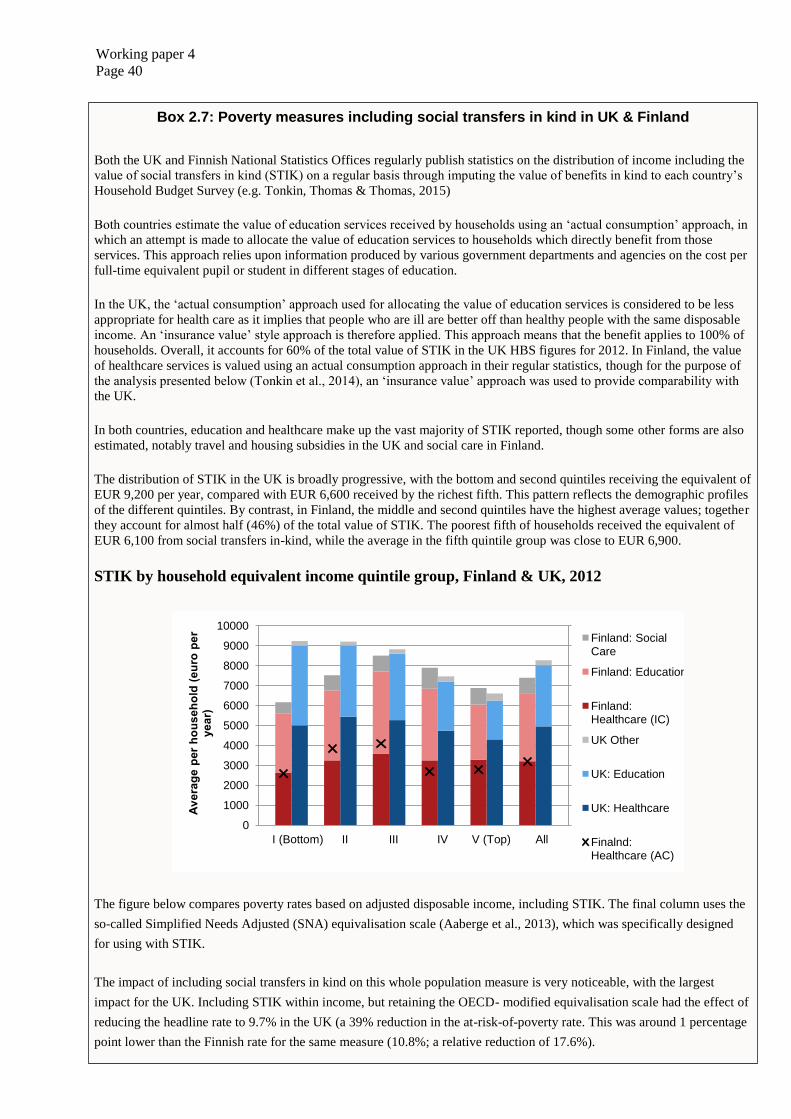
Working paper 4
Page 40
Box 2.7: Poverty measures including social transfers in kind in UK & Finland
Both the UK and Finnish National Statistics Offices regularly publish statistics on the distribution of income including the
value of social transfers in kind (STIK) on a regular basis through imputing the value of benefits in kind to each country’s
Household Budget Survey (e.g. Tonkin, Thomas & Thomas, 2015)
Both countries estimate the value of education services received by households using an ‘actual consumption’ approach, in
which an attempt is made to allocate the value of education services to households which directly benefit from those
services. This approach relies upon information produced by various government departments and agencies on the cost per
full-time equivalent pupil or student in different stages of education.
In the UK, the ‘actual consumption’ approach used for allocating the value of education services is considered to be less
appropriate for health care as it implies that people who are ill are better off than healthy people with the same disposable
income. An ‘insurance value’ style approach is therefore applied. This approach means that the benefit applies to 100% of
households. Overall, it accounts for 60% of the total value of STIK in the UK HBS figures for 2012. In Finland, the value
of healthcare services is valued using an actual consumption approach in their regular statistics, though for the purpose of
the analysis presented below (Tonkin et al., 2014), an ‘insurance value’ approach was used to provide comparability with
the UK.
In both countries, education and healthcare make up the vast majority of STIK reported, though some other forms are also
estimated, notably travel and housing subsidies in the UK and social care in Finland.
The distribution of STIK in the UK is broadly progressive, with the bottom and second quintiles receiving the equivalent of
EUR 9,200 per year, compared with EUR 6,600 received by the richest fifth. This pattern reflects the demographic profiles
of the different quintiles. By contrast, in Finland, the middle and second quintiles have the highest average values; together
they account for almost half (46%) of the total value of STIK. The poorest fifth of households received the equivalent of
EUR 6,100 from social transfers in-kind, while the average in the fifth quintile group was close to EUR 6,900.
STIK by household equivalent income quintile group, Finland & UK, 2012
The figure below compares poverty rates based on adjusted disposable income, including STIK. The final column uses the
so-called Simplified Needs Adjusted (SNA) equivalisation scale (Aaberge et al., 2013), which was specifically designed
for using with STIK.
The impact of including social transfers in kind on this whole population measure is very noticeable, with the largest
impact for the UK. Including STIK within income, but retaining the OECD- modified equivalisation scale had the effect of
reducing the headline rate to 9.7% in the UK (a 39% reduction in the at-risk-of-poverty rate. This was around 1 percentage
point lower than the Finnish rate for the same measure (10.8%; a relative reduction of 17.6%).
31.7.2014
20(43)
IARIW2014_UK&FI_STIK_FINAL.docx
This figure also highlights the differing distribution of STIK across quintiles in the UK and
Finnish data. Based on this data, the distribution of STIK in the UK is broadly progressive,
with the bottom and second quintiles receiving the equivalent of EUR 9,200 per year,
compared with EUR 6,600 received by the richest fifth. This pattern reflects the
demographic profiles of the different quintiles.
The value of healthcare is lower in the top two quintiles in the UK, as those over the age of
65, who on average make greater use of health services, are largely located in the bottom
three income quintiles. Similarly, households in the lower quintile groups received the
highest benefit from education. This is due to the relatively high number of children in this
part of the distribution, along with the presence of university/college students living in shared
houses. In addition, children in households in the higher quintiles are more likely to be
attending private schools and an allocation is not made in these cases.
Figure 4.1: Social transfers in kind by household equivalent income quintile
group, Finland & UK, HBS 2012.
By contrast, in Finland, the middle and second quintiles have the highest average values;
together they account for almost half (46%) of the total value of STIK. The poorest fifth of
households received the equivalent of EUR 6,100 from social transfers in-kind, while the
average in the fifth quintile group was close to EUR 6,900. The middle quintile received the
highest benefit from both education and healthcare. Social services are more concentrated
to the fourth and fifth quintile.
The crosses in Figure 4.1 show the average value of health services when imputed with the
actual consumption approach (AC). The actual consumption method allocates more value to
the second and third quintiles and less to the fourth and fifth compared to the insurance
approach (IC). The average value in the bottom fifth remains almost unchanged.
Figure 4.2 summarises the effect that these social transfers in kind has on the income
distributions for the UK and Finland. In this chart, primary income is defined as income from
0
1000
2000
3000
4000
5000
6000
7000
8000
9000
10000
I (Bottom) II III IV V (Top) All
Av
era
ge
per
ho
us
eh
old
(eu
ro p
er
ye
ar)
Finland: Social Care
Finland: Education
Finland: Healthcare (IC)
UK Other
UK: Education
UK: Healthcare
Finalnd: Healthcare (AC)
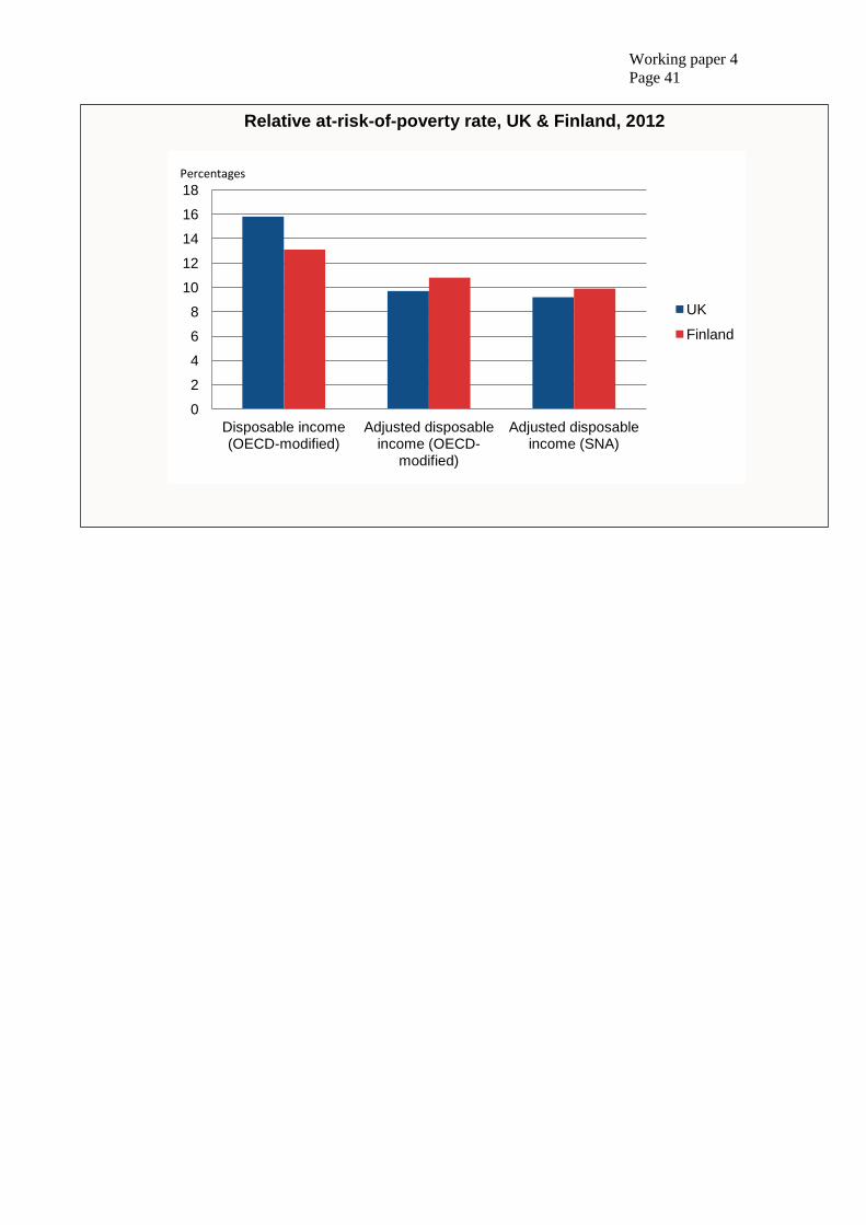
Working paper 4
Page 41
Relative at-risk-of-poverty rate, UK & Finland, 2012
31.7.2014
28(43)
IARIW2014_UK&FI_STIK_FINAL.docx
(a 39% reduction in the at-risk-of-poverty rate. This was around 1 percentage point lower
than the Finnish rate for the same measure (10.8%; a relative reduction of 17.6%).
Figure 4.4: Relative at-risk-of-poverty rates, UK and Finland, 2012
For the overall population, the effect of applying the SNA equivalisation scale was relatively
small, reducing the relative at-risk-of-poverty rate for adjusted disposable income to 9.2% in
the UK and 9.9% in Finland.
For reference, Table 4.4.1 also shows the estimates of Aaberge et. al. (2013), who imputed
social transfers in kind to all European countries using EU-SILC data. According to
Aaberge, in 2009 social transfers in kind reduced poverty rate by 33 % (5.8 pp) in the UK
and by 28 % (3.6 pp) in Finland, using the modified OECD scale. In both countries, the SNA
scale further reduced poverty rates.
In Finland, the HBS poverty rate is reduced by 17.5 percent (2.3 pp) with the insurance-
based health care while it only reduces by 4.5 % (0.6 pp) with the actual consumption
approach. The results suggest that insurance-based imputation of health care has more
impact on income poverty and inequality than actual consumption based imputation.
Compared to Aaberge et. al., the decrease in poverty is smaller. This result may be driven
by differences in data sources, reference years, and methods.
The different impact of STIK on poverty measures in Finland and the UK may be partly
explained by the composition of the population at risk of poverty under the disposable
income measure. If the beneficiaries of education and healthcare services are more likely to
be clustered around the middle of the income distribution (as is the case in Finland - see
Figure 4.1) then any reduction in poverty rates due to the inclusion of STIK is likely to be
relatively small compared with a country such as the UK, where those towards the bottom of
the income distribution typically benefit from STIK the most.
0
2
4
6
8
10
12
14
16
18
Disposable income (OECD-modified)
Adjusted disposable income (OECD-
modified)
Adjusted disposable income (SNA)
UK
Finland
Percentages
Working paper 4
Page 42
Box 2.8: The measurement of imputed rents and social transfers in kind in the
OECD
The issue of including imputed rents and social transfers in kind (STIKs) in national measures of income is of
great importance to poverty and income distribution studies and matters a lot for guiding policy-making.
In 2001, the first edition of the Canberra Group Handbook included imputed rent in the conceptual definition of
income but not in the operational one, mainly due to methodological concerns and the lack of harmonised and
comparable data. However, in 2011, in the 2nd edition of the Handbook, the operational definition of income was
broadened up as to include the net value of owner-occupied housing services in the recommended income
definition to be used for international comparisons.
As for STIKs, both editions of the Handbook acknowledged the importance of adding the value of STIKs to
household disposable income to create a measure of adjusted disposable income. The 2011 edition of the
Handbook also stressed that “the development of comparable estimates of STIKs should have high priority if the
accuracy as well as the international comparability of income distribution statistics is to be improved”.
In practice, however, due to measurement challenges and methodological concerns, available international
evidence on levels and trends in income inequalities and poverty usually keep relying on the concept of
household disposable cash income, thus ignoring the services from owner-occupied dwellings and the services
that governments provide to households. At the European level, imputed rent and STIKs are not included in the
standard definition of income underpinning the main indicator of risk of poverty. Similarly, they are not included
in the income definition underpinning the indicators of the OECD Income Distribution Database.
In 2015, the OECD sent a questionnaire to its network of income data providers, aiming to collecting information
on what statistical offices and other data producers have done, are doing, and are planning to do in terms of
including imputed rents and social transfers in kind in their measures of income inequality. To date the OECD
received replies from 27 countries, which show the interest that national statistical offices give to this area of
work. A brief overview of the main results of the OECD questionnaire is provided here, while a more detailed
analysis can be found in Balestra and Sustova (forthcoming).
Only 3 out of 27 countries (Canada, Korea and the United States) do not compute imputed rent. Most countries
produce and disseminate such estimates annually, with 2013 and 2014 being reported as the most frequent ‘latest
year of estimate’. The rental equivalence approach is used by the large majority of countries, and implemented
through different methods - including the stratification method, the hedonic and linear regression methods, the
subjective method as well as a mix of different methods. Most countries do not plan to change measurement
approach/method in the near future, either because the current one is delivering satisfactory results or because
they want to avoid breaks in series.
Half of the countries producing estimates of imputed rent include them in national definitions of income: 5
include imputed rent in the main national concept of income, 7 in secondary or alternative ones. The inclusion of
imputed rent in the operational income definition produces different effects on poverty rates: poverty decreases in
a small majority of countries, while it increases in Austria, Finland, France, Mexico and Norway. The impact also
varies across different population groups.
Only 30% of the countries that answered the questionnaire are computing estimates of social transfers in kind
(STIKs). The majority of countries produce and disseminate such estimates regularly – two to five years is the
most frequent periodicity for publication of the estimates. All countries include healthcare benefits in their

Working paper 4
Page 43
estimates of STIKs, almost all of them include education and childcare, and a majority also include long-term
services for the elderly. Two countries (Australia and France) include social housing in the estimates, while
Norway includes subsidies for public transport, social services targeted towards disadvantaged individuals and
culture. As for the valuation methods used, countries can be grouped in three groups: those that use the average
cost of production approach, those that use the average cost of provision approach and those that use a mix of
these two approaches. 30% of countries allocate STIKs to beneficiaries (actual consumption approach), another
30% allocate the value of services equally among those having certain characteristics (insurance value approach),
while the remaining 40% use a combination of approaches. In most countries STIKs are attributed to the
individual beneficiaries, although in a few countries they are attributed to the household as a whole. Only 4 out of
the 10 countries that produce estimates of STIKs include their value when computing household income.
Estimates of STIKs vary from 7.1% of household cash disposable income in Mexico to up to 44% (if only the part
of public consumption that may be individualised is distributed) or 62% (if total public consumption is distributed
to individuals) 44% in Denmark. The average share is however lower – around one fifth to one fourth of
household cash disposable income. Half of countries reported a decrease in the level of national poverty rates due
to the inclusion of STIKs in the definition of income.
The 2016 EU-SILC ad hoc module on access to services could potentially help to make the imputation of STIKs
more accurate. The module focuses on the affordability of services, and on the unmet needs for such services;
questions on proportion of cost of these services paid by households are also included, which could help identify
the exact amount of social transfers in kind to allocate to a particular household. The ad hoc module considers the
following services: are childcare, formal education and training, lifelong learning, healthcare and professional
homecare.
Working paper 4
Page 44
Section C: Setting a poverty line
1. Absolute vs. Relative poverty lines
As described in previous sections, an individual or household is classified as poor (or at risk of
poverty) if its resources are less than the value of a given monetary threshold (“poverty line”). The
poverty line represents the aggregate value of all the goods and services considered necessary to
satisfy the household’s basic needs.
Regarding the establishment of the poverty line, three basic approaches can be identified:
The absolute poverty line (or “having less than an objectively defined absolute minimum”,
Hagenaars & De Vos, 1987)
The relative poverty line (or “having less than others)”
The subjective poverty line (or “feeling you do not have enough to get along”
The first two of these approaches are the primary focus of this chapter. Subjective poverty, which is
not necessarily an alternative to objective poverty, but rather is complementary, is dealt with in
Chapter 31.
In setting a poverty line, the definition of what can be considered “good practice” should take the
following points into account:
a) Is there a clear definition of the relevant standard and its units of measurement?
b) Is it based on an existing source of information that meets minimum quality standards?
c) Has it been applied more than once, ideally for the same country or region? If, however,
calculations have been carried out only once but for many countries, then they may still
qualify;
d) Does it produce information that is a useful input for public policies or that is related to
aspects falling within the purview of those policies.
Almost all countries with official measures of poverty, base these on either absolute and relative
poverty lines and consequently poverty indicators according to these lines.
2. Absolute Poverty Lines
Strictly speaking, the absolute measures include all methods to estimate poverty which do not depend
on the average condition of the population.
Absolute poverty lines are by far the most commonly used approach for identifying the poor over time
and space and are universally used in low and middle-income countries. They allow transparent
comparisons where the changes in measured poverty can be attributed purely to changes in the
distribution rather than to a moving poverty cut-off.
Perhaps the most common approach to establishing an absolute poverty line involves determining the
monetary value of a set of goods and services considered essential to achieve a minimally acceptable
standard of living.
There are some important practical challenges associated with the construction of absolute poverty
lines using such an approach. First, it is unrealistic to maintain the composition of this basket of
“essential” goods and services as fixed over time and across countries and regions. The resources that
might be considered essential in terms of food, clothing and housing in the early part of the 20th
1 Subjective poverty measures, based on respondents own perceptions of the minimum income needed to get by are distinct from absolute
poverty lines set using subjective assessments of what is an acceptable minimum. The latter is dealt with later in this chapter.
Working paper 4
Page 45
Century are likely to be substantially different to what is deemed vital today - as a result of benefits
brought by technological advances and the general improvement of living conditions – in order to
reach a decent standard of living.
There is therefore an important question of how frequently to update an absolute poverty line. But
here the trade-offs are clear: it must be fixed long enough to be able to discern the underlying changes
in poverty, and it must be updated often enough so that the standard is reasonably consistent with
prevailing circumstances.
Absolute poverty lines are often held constant over many periods, and then updated to reflect
changing living standards. After updating of lines, comparisons are typically not made across the two
standards. Instead, each distribution is evaluated at the new, updated poverty line. The U.S. poverty
line has remained fixed (in real terms) since 1965 (see Box 2.9); the nominal poverty line is adjusted
for inflation. The World Bank’s main poverty standard was updated in 2015, and all income
distributions back to 1981 were re-evaluated at the new line.
Although absolute poverty lines are most commonly used in countries in the developing world, there
are a number of reasons for using such an approach in all countries. First of all, although there
proportion of the population in absolute poverty in developed countries may be very small, it is
important to understand the characteristics of those who are, in order to effectively target welfare
policies. Additionally, an absolute poverty line is effective for use in evaluating poverty within a
country over short-to-moderate spans of time or across two countries when they have roughly similar
levels of development. The approach may be harder to justify over longer periods of time or in a
comparison of countries with very different levels of development.
a) Setting absolute poverty lines
The way in which national statistical offices and others set absolute poverty lines varies considerably
across countries. As stated above, the cost of basic needs approach is most commonly used,
particularly in developing countries, but the variations in the application of the approach multiply with
each step. It first estimates the cost of acquiring enough food for adequate nutrition, with pre-defined
certain amount of Calories per equivalent adult per day and then adds the cost of other essentials such
as clothing and shelter.
This approach is based on expenditure data rather than income data.
b) Cost of Basic needs approach
i) Specify a food poverty threshold
The food poverty lines are based on minimum nutritional requirements. A person is counted as food
poor if the nutritional content of the food(s) they consume is less than the prescribed threshold. As a
simplifying assumption, mostly used dietary energy as a proxy for overall nutritional status, i.e., if a
person gets enough energy, then it is assumed that they obtain adequate protein and the other essential
nutrients.
ii) Food basket construct and food poverty line (fpl)
To determine the cost of the food basket, two different procedures can be identified: constructing an
explicit food basket and then pricing it, or estimating the cost of the food basket without listing its
contents.
A. Constructing an explicit food basket. Under this approach for computing the food poverty
line, an explicit bundle of food by item and weight are needed. (for example, meat - 0.25kg,
Working paper 4
Page 46
sugar - 0.03 kg, etc), which provides a total close to the specified threshold (in kcal per
equivalent adult per day). The conversion is made through a so-called food composition table,
which varies across individual countries to reflect their individual situations. The composition
of the food basket depends on the choice of reference population. Since the object is to
identify and count the poor, the reference population is usually some lower percentile of
households according to their equivalent adult consumption expenditure distribution. The
choice of the percentile cut-off point is usually guided by the most recent poverty incidence
estimates, what infers that, the reference population should be similar to the poor population;
B. Price per kcalorie. This method avoids constructing a food basket by instead calculating the
total expenditure and total kcal content of all the food consumed by the reference population.
The ratio between the two totals is a price per kcal estimate. When this figure is multiplied by
the energy threshold, it provides an estimate of fpl. Once a price-per-kcal estimate is
calculated, fpl's for as many choices of energy thresholds are easily computed. However, the
approach requires as many food expenditures and conversion into energy equivalents as there
are food commodities consumed by the reference population.
iii) Computing the total poverty line (tpl)
This computation involves two steps. The first defines essential non-food basic needs and the second
incorporates their cost into the food poverty line (fpl) to arrive at the total poverty line (tpl).
Essentially, the fpl has to be adjusted upward by an amount equal to or proportionate to the cost of
procuring the essential non-food basic needs of a poor or nearly poor person. Therefore, essential non-
food basic needs requires a definition that can be measured. Developing countries generally follow
one of two operational definitions or procedures:
A. List of specified essential non-food needs. This list is created usually by a group of users and
stakeholders in association with the national statistics office or the agency charged with
producing the country's official poverty statistics. The list is exhaustive, covering items like
clothing and footwear, shelter, fuel and light, household goods, health services, personal care,
and education. Costs per person are assigned to each item. Hence, if nfpl (non-food poverty
line) denotes the sum of the costs, then tpl = fpl + nfpl. However, the outcome is very much
dependent on a highly subjective list. Adding or subtracting from the list affects tpl directly in
an additive fashion. It is easy for anyone to criticize why this item is included while that item
is not;
B. Engel-coefficient. The most commonly used approach for drawing the non-food poverty line
is based on the observed Engel-coefficient (the proportion of expenditure devoted to food) for
a reference group of the population. The approach consists in multiplying the inverse of this
coefficient by the cost of the food basket, such that the non-food basket cost is directly
obtained from the consumption habits of the reference population. This methodology is based
on the original work done by Mollie Orshansky when drawing the U.S. poverty lines; it is
therefore sometimes referred to as the Orshansky multiplier. It is also possible to select
another reference group for the construction of the non-food poverty line, such as households
with a level of total expenditure close to the food poverty line.
By following a procedure based on the above methods, both a food poverty line and total poverty line
can be obtained. Poverty indicators are discussed in detail in the next section, but essentially, a person
is considered to be poor if his households’ consumption expenditure per equivalent adult is less than
the total poverty line.
The total poverty line (tpl) is updated for future years using a measure of price change such as the
Consumer Price Index (CPI).
Working paper 4
Page 47
Pros:
Thresholds are defined directly from surveys;
Data are comparable over short-to-moderate spans of time.
Cons:
The CPI as currently constructed in most countries might not reflect the consumption pattern
of the reference population used in determining the poverty lines;
Depends on the initial calculation point – depending on point in time when the poverty
threshold is calculated, the poverty indicators are changing although the tendency stays the
same;
There is the related question of how frequently to update the poverty line. But here the trade-
offs are clear: it must be fixed long enough to be able to discern the underlying changes in
poverty, and it must be updated often enough so that the standard is reasonably consistent
with prevailing circumstances. Similar to any absolute poverty measurement, the poverty line
is often held constant over many periods, then updated to reflect changing living standards.
After updating of line, comparisons are typically not made across the two standards.
Estimates of the energy (caloric) requirements for the population are generally based on
internationally agreed recommendations (FAO/WHO), but energy (caloric) requirements used
by the countries differ, which leads to comparability issue.
c) Absolute poverty with respect to subsistence minimum
Another method used for constructing absolute poverty lines is subsistence minimum, used mainly in
CIS countries. For calculating the subsistence minimum, calculation of both food and non-food
components are needed.
i) calculation of food component or food poverty line (fpl)
The subsistence minimum is defined on the basis of a minimum food basket. The minimum food
basket represents a table of defined quantities of food products and contains the amount of food that is
physiologically required (proteins, fats and carbohydrates) for an equivalent adult to lead a normal life
and have the ability to work, which is converted to certain amount of calories. Usually, the minimum
food basket is defined by the Ministry of Health or relevant agency. Initially the cost of each
component of the minimum food basket is calculated by means of average food prices. Monthly cost
of a food basket product is obtained by multiplying a product’s monthly norm by its average price.
The sum of the costs for all food basket products represents a monthly cost of minimum food basket.
ii) calculation of the total poverty line (tpl)
This computation involves two steps. The first defines essential non-food basic needs and the second
incorporates their cost into the food poverty line (fpl) to arrive at the total poverty line (tpl). Simply
put, fpl has to be adjusted upward by an amount equal to or proportionate to the cost of procuring the
essential non-food basic needs of a poor or nearly poor person. Clearly, essential non-food basic needs
requires a definition that can be measured. Countries generally follow one of two operational
definitions or procedures:
A. List of specified essential non-food needs. This list is created usually by a group of users and
stakeholders in association with the national statistics office or the agency charged with
producing the country's official poverty statistics. The list is exhaustive, covering items like
clothing and footwear, shelter, fuel and light, household goods, health services, personal care,
and education. Costs per person are assigned to each item. Hence, if nfpl (non-food poverty
line) denotes the sum of the costs, then tpl = fpl + nfpl. However, the outcome is very much
dependent on a highly subjective list. Adding or subtracting from the list affects tpl directly in
Working paper 4
Page 48
an additive fashion. It is easy for anyone to criticize why this item is included while that item
is not;
B. Use coefficient from an ongoing household survey. The approach consists in multiplying the
inverse of the coefficient by the cost of the food basket (the share of food expenditure from
total household consumption expenditure derived from an ongoing household survey. Here
the reference population is usually some lower percentile of households according to their
equivalent adult consumption expenditure distribution. The choice of the percentile cut-off
point is usually guided by the most recent poverty incidence estimates, what infers that, the
reference population should be similar to the poor population) to calculate the subsistence
minimum or total poverty line (tpl). The obtained amount represents the final value of the
subsistence minimum for an equivalent adult in a given month.
As with the costs of basic needs approach, both a food poverty line and total poverty line can be
obtained, with the potential to identify those in poverty in the same manner.
With this approach, the total poverty line is updated monthly by calculating the cost of the subsistence
minimum on a monthly basis.
Disadvantages of the method:
Threshold is not defined from any survey;
Basket of goods used for the CPI may vary significantly from the one used to construct the
poverty lines;
Changes in prices (inflation) are not in direct proportion to the population’s (especially to the
poor population) welfare. In the situation when the prices on certain products given in the
minimum food basket are going up the threshold (subsistence minimum) increases as well,
even though the poor households could switch to cheaper food products of a similar nature;
Seasonality of food products that are given in the minimum food basket.
If we exclude measures applied for developing countries, the most consolidated and lasting
experiences conducted in developed economies are those measured produced in the United States
(Box 2.9) and Canada (Box 2.10). Additionally, Box 2.11 described the absolute poverty measure
introduced in Italy in 2005, which is disseminated on an annual basis.
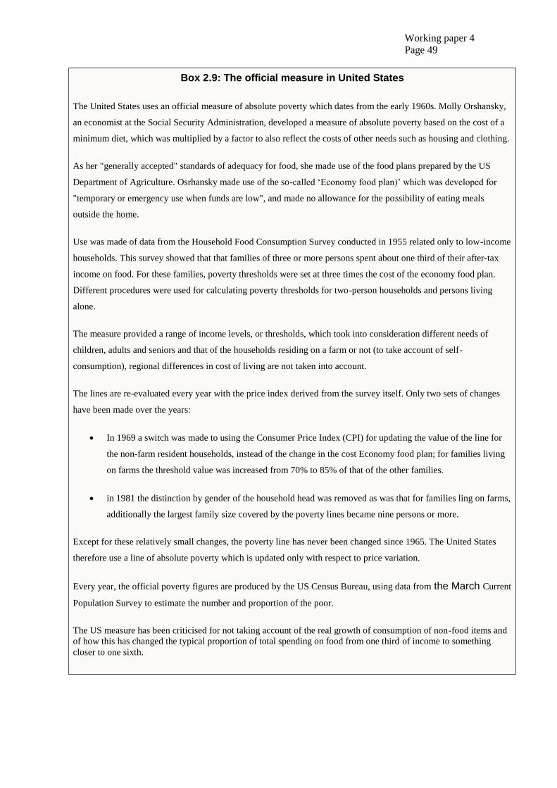
Working paper 4
Page 49
Box 2.9: The official measure in United States
The United States uses an official measure of absolute poverty which dates from the early 1960s. Molly Orshansky,
an economist at the Social Security Administration, developed a measure of absolute poverty based on the cost of a
minimum diet, which was multiplied by a factor to also reflect the costs of other needs such as housing and clothing.
As her "generally accepted" standards of adequacy for food, she made use of the food plans prepared by the US
Department of Agriculture. Osrhansky made use of the so-called ‘Economy food plan)’ which was developed for
"temporary or emergency use when funds are low", and made no allowance for the possibility of eating meals
outside the home.
Use was made of data from the Household Food Consumption Survey conducted in 1955 related only to low-income
households. This survey showed that that families of three or more persons spent about one third of their after-tax
income on food. For these families, poverty thresholds were set at three times the cost of the economy food plan.
Different procedures were used for calculating poverty thresholds for two-person households and persons living
alone.
The measure provided a range of income levels, or thresholds, which took into consideration different needs of
children, adults and seniors and that of the households residing on a farm or not (to take account of self-
consumption), regional differences in cost of living are not taken into account.
The lines are re-evaluated every year with the price index derived from the survey itself. Only two sets of changes
have been made over the years:
In 1969 a switch was made to using the Consumer Price Index (CPI) for updating the value of the line for
the non-farm resident households, instead of the change in the cost Economy food plan; for families living
on farms the threshold value was increased from 70% to 85% of that of the other families.
in 1981 the distinction by gender of the household head was removed as was that for families ling on farms,
additionally the largest family size covered by the poverty lines became nine persons or more.
Except for these relatively small changes, the poverty line has never been changed since 1965. The United States
therefore use a line of absolute poverty which is updated only with respect to price variation.
Every year, the official poverty figures are produced by the US Census Bureau, using data from the March Current
Population Survey to estimate the number and proportion of the poor.
The US measure has been criticised for not taking account of the real growth of consumption of non-food items and
of how this has changed the typical proportion of total spending on food from one third of income to something
closer to one sixth.
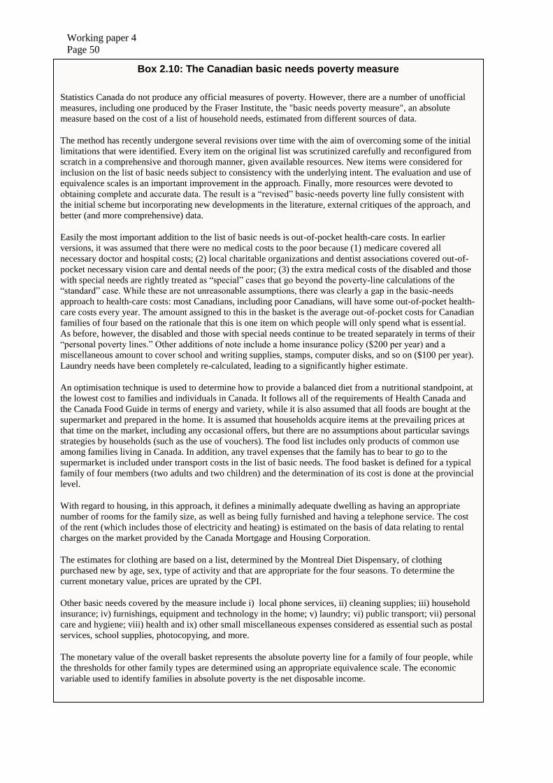
Working paper 4
Page 50
Box 2.10: The Canadian basic needs poverty measure
Statistics Canada do not produce any official measures of poverty. However, there are a number of unofficial
measures, including one produced by the Fraser Institute, the "basic needs poverty measure", an absolute
measure based on the cost of a list of household needs, estimated from different sources of data.
The method has recently undergone several revisions over time with the aim of overcoming some of the initial
limitations that were identified. Every item on the original list was scrutinized carefully and reconfigured from
scratch in a comprehensive and thorough manner, given available resources. New items were considered for
inclusion on the list of basic needs subject to consistency with the underlying intent. The evaluation and use of
equivalence scales is an important improvement in the approach. Finally, more resources were devoted to
obtaining complete and accurate data. The result is a “revised” basic-needs poverty line fully consistent with
the initial scheme but incorporating new developments in the literature, external critiques of the approach, and
better (and more comprehensive) data.
Easily the most important addition to the list of basic needs is out-of-pocket health-care costs. In earlier
versions, it was assumed that there were no medical costs to the poor because (1) medicare covered all
necessary doctor and hospital costs; (2) local charitable organizations and dentist associations covered out-of-
pocket necessary vision care and dental needs of the poor; (3) the extra medical costs of the disabled and those
with special needs are rightly treated as “special” cases that go beyond the poverty-line calculations of the
“standard” case. While these are not unreasonable assumptions, there was clearly a gap in the basic-needs
approach to health-care costs: most Canadians, including poor Canadians, will have some out-of-pocket health-
care costs every year. The amount assigned to this in the basket is the average out-of-pocket costs for Canadian
families of four based on the rationale that this is one item on which people will only spend what is essential.
As before, however, the disabled and those with special needs continue to be treated separately in terms of their
“personal poverty lines.” Other additions of note include a home insurance policy ($200 per year) and a
miscellaneous amount to cover school and writing supplies, stamps, computer disks, and so on ($100 per year).
Laundry needs have been completely re-calculated, leading to a significantly higher estimate.
An optimisation technique is used to determine how to provide a balanced diet from a nutritional standpoint, at
the lowest cost to families and individuals in Canada. It follows all of the requirements of Health Canada and
the Canada Food Guide in terms of energy and variety, while it is also assumed that all foods are bought at the
supermarket and prepared in the home. It is assumed that households acquire items at the prevailing prices at
that time on the market, including any occasional offers, but there are no assumptions about particular savings
strategies by households (such as the use of vouchers). The food list includes only products of common use
among families living in Canada. In addition, any travel expenses that the family has to bear to go to the
supermarket is included under transport costs in the list of basic needs. The food basket is defined for a typical
family of four members (two adults and two children) and the determination of its cost is done at the provincial
level.
With regard to housing, in this approach, it defines a minimally adequate dwelling as having an appropriate
number of rooms for the family size, as well as being fully furnished and having a telephone service. The cost
of the rent (which includes those of electricity and heating) is estimated on the basis of data relating to rental
charges on the market provided by the Canada Mortgage and Housing Corporation.
The estimates for clothing are based on a list, determined by the Montreal Diet Dispensary, of clothing
purchased new by age, sex, type of activity and that are appropriate for the four seasons. To determine the
current monetary value, prices are uprated by the CPI.
Other basic needs covered by the measure include i) local phone services, ii) cleaning supplies; iii) household
insurance; iv) furnishings, equipment and technology in the home; v) laundry; vi) public transport; vii) personal
care and hygiene; viii) health and ix) other small miscellaneous expenses considered as essential such as postal
services, school supplies, photocopying, and more.
The monetary value of the overall basket represents the absolute poverty line for a family of four people, while
the thresholds for other family types are determined using an appropriate equivalence scale. The economic
variable used to identify families in absolute poverty is the net disposable income.
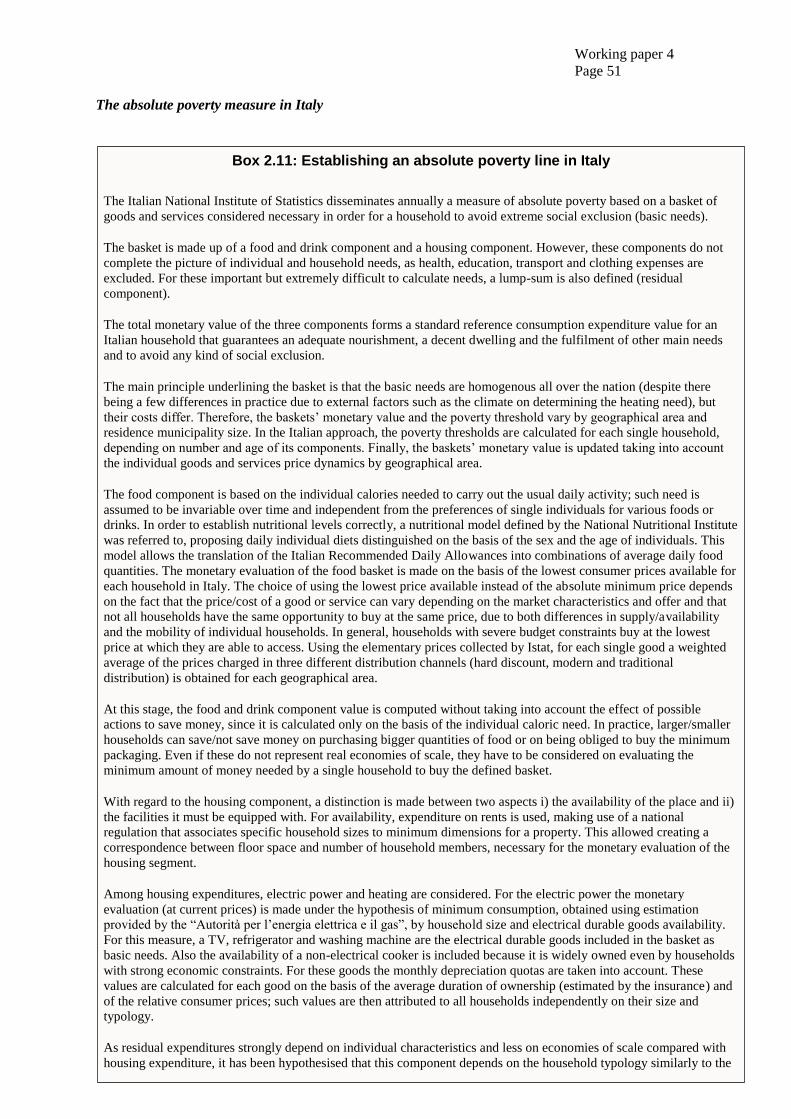
Working paper 4
Page 51
The absolute poverty measure in Italy
Box 2.11: Establishing an absolute poverty line in Italy
The Italian National Institute of Statistics disseminates annually a measure of absolute poverty based on a basket of
goods and services considered necessary in order for a household to avoid extreme social exclusion (basic needs).
The basket is made up of a food and drink component and a housing component. However, these components do not
complete the picture of individual and household needs, as health, education, transport and clothing expenses are
excluded. For these important but extremely difficult to calculate needs, a lump-sum is also defined (residual
component).
The total monetary value of the three components forms a standard reference consumption expenditure value for an
Italian household that guarantees an adequate nourishment, a decent dwelling and the fulfilment of other main needs
and to avoid any kind of social exclusion.
The main principle underlining the basket is that the basic needs are homogenous all over the nation (despite there
being a few differences in practice due to external factors such as the climate on determining the heating need), but
their costs differ. Therefore, the baskets’ monetary value and the poverty threshold vary by geographical area and
residence municipality size. In the Italian approach, the poverty thresholds are calculated for each single household,
depending on number and age of its components. Finally, the baskets’ monetary value is updated taking into account
the individual goods and services price dynamics by geographical area.
The food component is based on the individual calories needed to carry out the usual daily activity; such need is
assumed to be invariable over time and independent from the preferences of single individuals for various foods or
drinks. In order to establish nutritional levels correctly, a nutritional model defined by the National Nutritional Institute
was referred to, proposing daily individual diets distinguished on the basis of the sex and the age of individuals. This
model allows the translation of the Italian Recommended Daily Allowances into combinations of average daily food
quantities. The monetary evaluation of the food basket is made on the basis of the lowest consumer prices available for
each household in Italy. The choice of using the lowest price available instead of the absolute minimum price depends
on the fact that the price/cost of a good or service can vary depending on the market characteristics and offer and that
not all households have the same opportunity to buy at the same price, due to both differences in supply/availability
and the mobility of individual households. In general, households with severe budget constraints buy at the lowest
price at which they are able to access. Using the elementary prices collected by Istat, for each single good a weighted
average of the prices charged in three different distribution channels (hard discount, modern and traditional
distribution) is obtained for each geographical area.
At this stage, the food and drink component value is computed without taking into account the effect of possible
actions to save money, since it is calculated only on the basis of the individual caloric need. In practice, larger/smaller
households can save/not save money on purchasing bigger quantities of food or on being obliged to buy the minimum
packaging. Even if these do not represent real economies of scale, they have to be considered on evaluating the
minimum amount of money needed by a single household to buy the defined basket.
With regard to the housing component, a distinction is made between two aspects i) the availability of the place and ii)
the facilities it must be equipped with. For availability, expenditure on rents is used, making use of a national
regulation that associates specific household sizes to minimum dimensions for a property. This allowed creating a
correspondence between floor space and number of household members, necessary for the monetary evaluation of the
housing segment.
Among housing expenditures, electric power and heating are considered. For the electric power the monetary
evaluation (at current prices) is made under the hypothesis of minimum consumption, obtained using estimation
provided by the “Autorità per l’energia elettrica e il gas”, by household size and electrical durable goods availability.
For this measure, a TV, refrigerator and washing machine are the electrical durable goods included in the basket as
basic needs. Also the availability of a non-electrical cooker is included because it is widely owned even by households
with strong economic constraints. For these goods the monthly depreciation quotas are taken into account. These
values are calculated for each good on the basis of the average duration of ownership (estimated by the insurance) and
of the relative consumer prices; such values are then attributed to all households independently on their size and
typology.
As residual expenditures strongly depend on individual characteristics and less on economies of scale compared with
housing expenditure, it has been hypothesised that this component depends on the household typology similarly to the
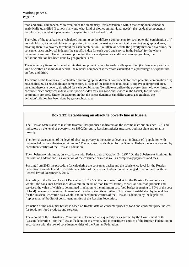
Working paper 4
Page 52
food and drink component. Moreover, since the elementary items considered within that component cannot be
analytically quantified (i.e. how many and what kind of clothes an individual needs), the residual component is
therefore calculated as a percentage of expenditure on food and drink.
The value of the total basket is calculated summing up the different components for each potential combination of i)
household size, ii) household age composition, iii) size of the residence municipality and iv) geographical area,
meaning there is a poverty threshold for each combination. To inflate or deflate the poverty threshold over time, the
consumer price analytical indexes (the specific index for each good and service in the basket) for the whole
community are used. Under the assumption that the prices dynamics can differ across geographies, the
deflation/inflation has been done by geographical area.
The elementary items considered within that component cannot be analytically quantified (i.e. how many and what
kind of clothes an individual needs), the residual component is therefore calculated as a percentage of expenditure
on food and drink.
The value of the total basket is calculated summing up the different components for each potential combination of i)
household size, ii) household age composition, iii) size of the residence municipality and iv) geographical area,
meaning there is a poverty threshold for each combination. To inflate or deflate the poverty threshold over time, the
consumer price analytical indexes (the specific index for each good and service in the basket) for the whole
community are used. Under the assumption that the prices dynamics can differ across geographies, the
deflation/inflation has been done by geographical area.
Box 2.12: Establishing an absolute poverty line in Russia
The Russian State statistics institute (Rosstat) has produced indicators on the income distribution since 1970 and
indicators on the level of poverty since 1990.Currently, Russian statistics measures both absolute and relative
poverty.
The Formal assessment of the level of absolute poverty at the national level is an indicator of "population with
incomes below the subsistence minimum." The indicator is calculated for the Russian Federation as a whole and by
constituent entities of the Russian Federation.
The subsistence minimum, in accordance with Federal Law of October 24, 1997 "On the Subsistence Minimum in
the Russian Federation", is a valuation of the consumer basket as well as compulsory payments and fees.
Starting from 2013 the procedure for calculating the consumer basket and the subsistence level for the Russian
Federation as a whole and by constituent entities of the Russian Federation was changed in accordance with the
Federal law of December 3, 2012.
According to the Federal Law of December 3, 2012 "On the consumer basket for the Russian Federation as a
whole", the consumer basket includes a minimum set of food (in real terms), as well as non-food products and
services, the value of which is determined in relation to the minimum cost food basket (equating to 50% of the cost
of food) necessary to maintain human health and ensuring its activities. This basket is established by federal law
for the Russian Federation as a whole, and in constituent entities of the Russian Federation by the legislative
(representative) bodies of constituent entities of the Russian Federation.
Valuation of the consumer basket is based on Rosstat data on consumer prices of food and consumer price indices
for food, non-food products and services.
The amount of the Subsistence Minimum is determined on a quarterly basis and set by the Government of the
Russian Federation – for the Russian Federation as a whole, and in constituent entities of the Russian Federation in
accordance with the law of constituent entities of the Russian Federation.

Working paper 4
Page 53
3. Relative Poverty Lines
Relative poverty as a concept was first developed by Peter Townsend in the UK, who described
people as being in poverty when “they lack the resources to obtain the type of diet, participate in the
activities and have the living conditions and the amenities which are customary, or at least widely
encouraged or approved in the societies to which they belong. Their resources are so seriously below
those commanded by the average family that they are in effect excluded from the ordinary living
patterns, customs, and activities” (Townsend, 1979).
A relative poverty line is an explicit function of the income (or consumption expenditure) distribution,
namely, a constant fraction of some income standard. One example is the European Union’s country-
level poverty lines, which are set at 60 percent of a country’s median (disposable) income. The nature
of a relative poverty line dictates that the cut-off below which one is considered to be poor varies
proportionally with its income standard. Indeed, a level of income that is above the poverty line in one
distribution may lie below the poverty line of a second distribution having a higher income standard.
Relative poverty lines are most often used in countries with higher incomes, where there is less
concern about achieving a minimum absolute level of living and greater interest in inclusion or
relative achievements.
With a relative line, the analysis of a change in poverty over time (or space) is less transparent.
Moreover, if income of every household increases twice, the incidence of poverty calculated by the
relative line will remain the same, hence it represents not only poverty, but inequality as well. In
addition, if income of every household decreases (with different amount), the poverty incidence may
decrease as well as it depends on income distribution of the society.
A key advantage of a relative poverty is its conceptual clarity and simplicity of use (particularly for
international comparisons). However, any value of relative poverty essentially is arbitrary. Also,
unlike absolute, the relative poverty line will increase after a general increase in average incomes of
the society, and the process of poverty reduction will not be as obvious as in a absolute approach.
Given the advantages and disadvantages of both relative and absolute poverty measures, many
countries use both types of measure (as well as subjective measures in some cases) together in order
to gain a richer understanding of poverty in their country.
a. Mean vs median
The selection of the parameter to determine the value of the poverty line influences both the
interpretation and the measurement of the phenomenon.
If you consider the arithmetic mean, this, in addition to being straightforward to calculate, is the level
of income (consumption expenditure, welfare) all the households would have if resources were
equally distributed. This parameter, however, can be unstable, especially over time, as it is very
sensitive to extreme values of the distribution.
Another parameter, which is the one most commonly used for determining the poverty line is the
median. The median income is the household income of what would be the middle individual if all
individuals in the population were sorted in a list from poorest to richest. As it represents the middle
of the income distribution, the median household income provides a good indication of the standard of
living of the “typical” individual in terms of income. The median is the most stable among other
measures, and it is the most appropriate choice for a log-normal distribution (which often well
approximates the distribution of income or consumption expenditure) as separately for predicting the
effect of the economic cycle and inequality inside the distribution.
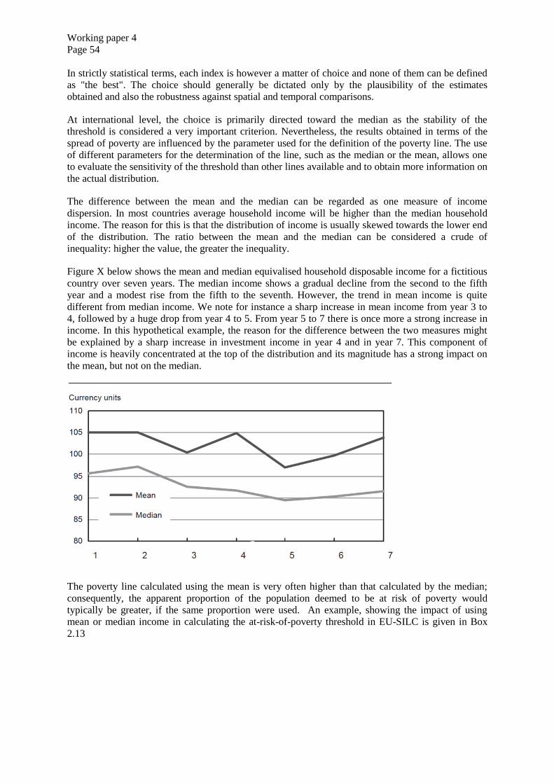
Working paper 4
Page 54
In strictly statistical terms, each index is however a matter of choice and none of them can be defined
as "the best". The choice should generally be dictated only by the plausibility of the estimates
obtained and also the robustness against spatial and temporal comparisons.
At international level, the choice is primarily directed toward the median as the stability of the
threshold is considered a very important criterion. Nevertheless, the results obtained in terms of the
spread of poverty are influenced by the parameter used for the definition of the poverty line. The use
of different parameters for the determination of the line, such as the median or the mean, allows one
to evaluate the sensitivity of the threshold than other lines available and to obtain more information on
the actual distribution.
The difference between the mean and the median can be regarded as one measure of income
dispersion. In most countries average household income will be higher than the median household
income. The reason for this is that the distribution of income is usually skewed towards the lower end
of the distribution. The ratio between the mean and the median can be considered a crude of
inequality: higher the value, the greater the inequality.
Figure X below shows the mean and median equivalised household disposable income for a fictitious
country over seven years. The median income shows a gradual decline from the second to the fifth
year and a modest rise from the fifth to the seventh. However, the trend in mean income is quite
different from median income. We note for instance a sharp increase in mean income from year 3 to
4, followed by a huge drop from year 4 to 5. From year 5 to 7 there is once more a strong increase in
income. In this hypothetical example, the reason for the difference between the two measures might
be explained by a sharp increase in investment income in year 4 and in year 7. This component of
income is heavily concentrated at the top of the distribution and its magnitude has a strong impact on
the mean, but not on the median.
The poverty line calculated using the mean is very often higher than that calculated by the median;
consequently, the apparent proportion of the population deemed to be at risk of poverty would
typically be greater, if the same proportion were used. An example, showing the impact of using
mean or median income in calculating the at-risk-of-poverty threshold in EU-SILC is given in Box
2.13
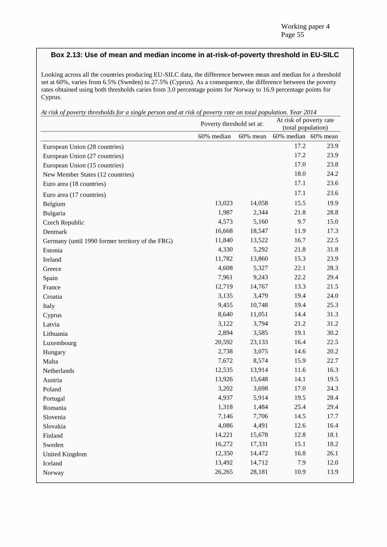
Working paper 4
Page 55
Box 2.13: Use of mean and median income in at-risk-of-poverty threshold in EU-SILC
Looking across all the countries producing EU-SILC data, the difference between mean and median for a threshold
set at 60%, varies from 6.5% (Sweden) to 27.5% (Cyprus). As a consequence, the difference between the poverty
rates obtained using both thresholds caries from 3.0 percentage points for Norway to 16.9 percentage points for
Cyprus.
At risk of poverty thresholds for a single person and at risk of poverty rate on total population. Year 2014
Poverty threshold set at:
At risk of poverty rate
(total population)
60% median 60% mean 60% median 60% mean
European Union (28 countries) 17.2 23.9
European Union (27 countries) 17.2 23.9
European Union (15 countries) 17.0 23.8
New Member States (12 countries) 18.0 24.2
Euro area (18 countries) 17.1 23.6
Euro area (17 countries) 17.1 23.6
Belgium 13,023 14,058 15.5 19.9
Bulgaria 1,987 2,344 21.8 28.8
Czech Republic 4,573 5,160 9.7 15.0
Denmark 16,668 18,547 11.9 17.3
Germany (until 1990 former territory of the FRG) 11,840 13,522 16.7 22.5
Estonia 4,330 5,292 21.8 31.8
Ireland 11,782 13,860 15.3 23.9
Greece 4,608 5,327 22.1 28.3
Spain 7,961 9,243 22.2 29.4
France 12,719 14,767 13.3 21.5
Croatia 3,135 3,479 19.4 24.0
Italy 9,455 10,748 19.4 25.3
Cyprus 8,640 11,051 14.4 31.3
Latvia 3,122 3,794 21.2 31.2
Lithuania 2,894 3,585 19.1 30.2
Luxembourg 20,592 23,133 16.4 22.5
Hungary 2,738 3,075 14.6 20.2
Malta 7,672 8,574 15.9 22.7
Netherlands 12,535 13,914 11.6 16.3
Austria 13,926 15,648 14.1 19.5
Poland 3,202 3,698 17.0 24.3
Portugal 4,937 5,914 19.5 28.4
Romania 1,318 1,484 25.4 29.4
Slovenia 7,146 7,706 14.5 17.7
Slovakia 4,086 4,491 12.6 16.4
Finland 14,221 15,678 12.8 18.1
Sweden 16,272 17,331 15.1 18.2
United Kingdom 12,350 14,472 16.8 26.1
Iceland 13,492 14,712 7.9 12.0
Norway 26,265 28,181 10.9 13.9

Working paper 4
Page 56
b. Level of threshold
Together with the selection of the parameter, also the choice of the fraction of the parameter itself
strongly influences the level of poverty estimation. Not only because higher is the fraction, the greater
is the poverty rate, but also because it depends on the distribution/concentration of the equivalent
distribution around the chosen value.
The most commonly used thresholds tend to be either 60% (used by Eurostat and many EU countries)
or 50% (used by the United Nations and the OECD, as well as individual countries) of the median
equivalised disposable income. The reasons these thresholds are commonly used are in part due to
comparability with the application of other approaches, and in part due to pragmatic considerations
such as measurement error and accepted practice.
The use of a single line of poverty can be complemented by additional thresholds (obtained as
percentage of the standard threshold) in order to highlight the sensitivity of the results to threshold
value. The additional thresholds allow to identify and analyse the characteristics of households closer
to the poverty line and those most exposed to the "risk" to elapse below. The application of different
poverty thresholds in EU-SILC is highlighted in box 2.14.
Box 2.14: Use of different threshold levels in EU-SILC
If we consider the European estimation of relative poverty, the incidence using a poverty line set at the 70% of the
median value is about 4 times that obtained by using the poverty line set at 40%. However, the relative ranking of
individual countries is very different: as an example, Malta, which shows the second lowest value if the threshold at
40% of the median is used, became the 19th if the threshold at 70% of the median is considered (the incidence
passes from 2.4% to 25.75). It means that a significant percentage of the population (almost 25%) has an equivalent
income very close to the 50% of the median value. The opposite case is represented by Romania, where the
incidence using the 70% poverty line is “only” 2.3 times that obtained by the 40% line; the percentage of population
with an equivalent income next to the half of the median value is about 17%, even if the incidences obtained are the
highest for any lines.
At risk of poverty thresholds for a single person and at risk of poverty rate on total population. Year 2014
Poverty threshold set at:
At risk of poverty rate
(total population)
40%
median
50%
median
60%
median
70%
median
40%
median
50%
median
60%
median
70%
median
European Union (28 countries)
6.3 10.8 17.2 24.9
European Union (27 countries)
6.3 10.8 17.2 24.9
European Union (15 countries)
6.0 10.4 17.0 24.8
New Member States (12 countries)
7.3 12.0 18.0 25.1
Euro area (18 countries)
6.3 10.7 17.1 24.7
Euro area (17 countries)
6.2 10.7 17.1 24.7
Belgium 8,682 10,852 13,023 15,193 3.8 8.6 15.5 24.9
Bulgaria 1,324 1,655 1,987 2,318 10.8 15.9 21.8 28.0
Czech Republic 3,049 3,811 4,573 5,336 2.4 5.2 9.7 17.0
Denmark 11,112 13,890 16,668 19,446 4.4 6.6 11.9 20.4
Germany (until 1990 former
territory of the FRG) 7,893 9,867 11,840 13,813 5.4 10.5 16.7 23.7
Estonia 2,887 3,609 4,330 5,052 7.9 13.0 21.8 29.0
Ireland 7,855 9,818 11,782 13,745 4.1 8.0 15.3 23.4
Greece 3,072 3,840 4,608 5,376 10.4 15.8 22.1 28.9
Spain 5,308 6,634 7,961 9,288 10.6 15.9 22.2 29.7
France 8,480 10,600 12,719 14,839 2.9 6.7 13.3 21.9
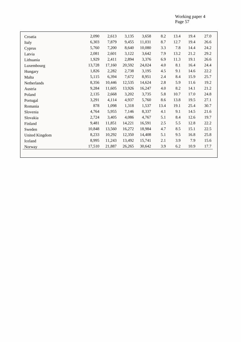
Working paper 4
Page 57
Croatia 2,090 2,613 3,135 3,658 8.2 13.4 19.4 27.0
Italy 6,303 7,879 9,455 11,031 8.7 12.7 19.4 26.6
Cyprus 5,760 7,200 8,640 10,080 3.3 7.8 14.4 24.2
Latvia 2,081 2,601 3,122 3,642 7.9 13.2 21.2 29.2
Lithuania 1,929 2,411 2,894 3,376 6.9 11.3 19.1 26.6
Luxembourg 13,728 17,160 20,592 24,024 4.0 8.1 16.4 24.4
Hungary 1,826 2,282 2,738 3,195 4.5 9.1 14.6 22.2
Malta 5,115 6,394 7,672 8,951 2.4 8.4 15.9 25.7
Netherlands 8,356 10,446 12,535 14,624 2.8 5.9 11.6 19.2
Austria 9,284 11,605 13,926 16,247 4.0 8.2 14.1 21.2
Poland 2,135 2,668 3,202 3,735 5.8 10.7 17.0 24.8
Portugal 3,291 4,114 4,937 5,760 8.6 13.8 19.5 27.1
Romania 878 1,098 1,318 1,537 13.4 19.1 25.4 30.7
Slovenia 4,764 5,955 7,146 8,337 4.1 9.1 14.5 21.6
Slovakia 2,724 3,405 4,086 4,767 5.1 8.4 12.6 19.7
Finland 9,481 11,851 14,221 16,591 2.5 5.5 12.8 22.2
Sweden 10,848 13,560 16,272 18,984 4.7 8.5 15.1 22.5
United Kingdom 8,233 10,292 12,350 14,408 5.1 9.5 16.8 25.8
Iceland 8,995 11,243 13,492 15,741 2.1 3.9 7.9 15.6
Norway 17,510 21,887 26,265 30,642 3.9 6.2 10.9 17.7
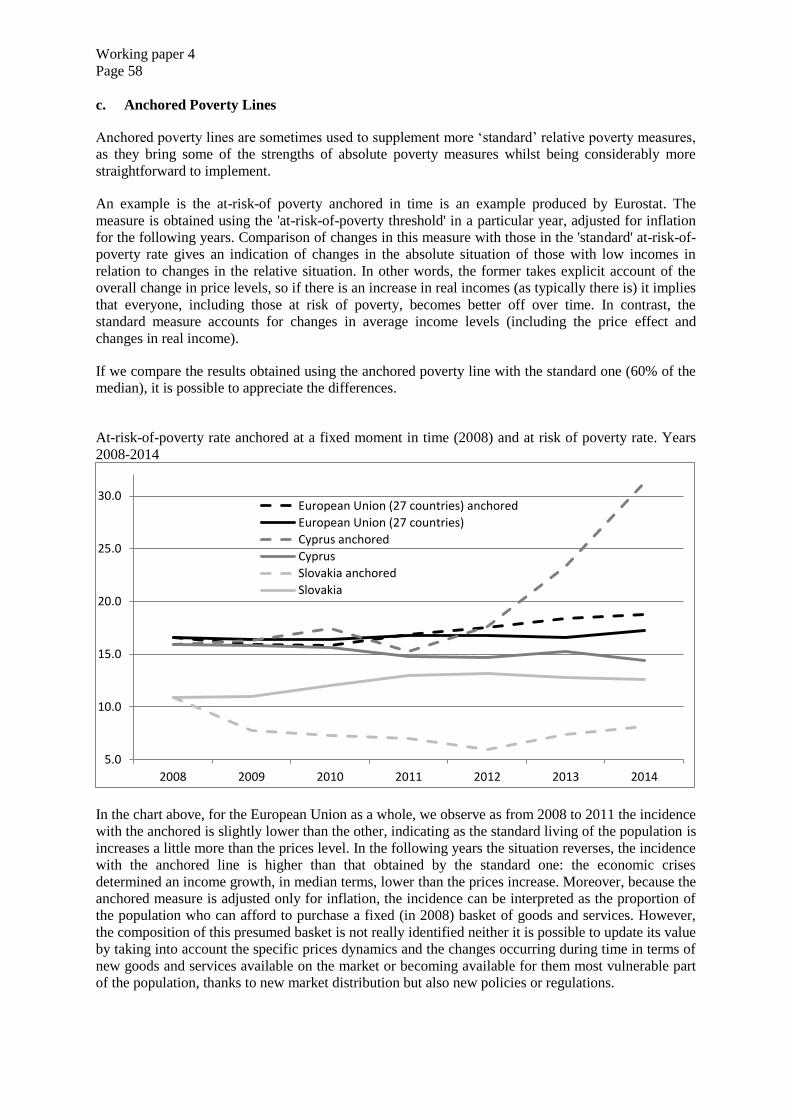
Working paper 4
Page 58
c. Anchored Poverty Lines
Anchored poverty lines are sometimes used to supplement more ‘standard’ relative poverty measures,
as they bring some of the strengths of absolute poverty measures whilst being considerably more
straightforward to implement.
An example is the at-risk-of poverty anchored in time is an example produced by Eurostat. The
measure is obtained using the 'at-risk-of-poverty threshold' in a particular year, adjusted for inflation
for the following years. Comparison of changes in this measure with those in the 'standard' at-risk-of-
poverty rate gives an indication of changes in the absolute situation of those with low incomes in
relation to changes in the relative situation. In other words, the former takes explicit account of the
overall change in price levels, so if there is an increase in real incomes (as typically there is) it implies
that everyone, including those at risk of poverty, becomes better off over time. In contrast, the
standard measure accounts for changes in average income levels (including the price effect and
changes in real income).
If we compare the results obtained using the anchored poverty line with the standard one (60% of the
median), it is possible to appreciate the differences.
At-risk-of-poverty rate anchored at a fixed moment in time (2008) and at risk of poverty rate. Years
2008-2014
In the chart above, for the European Union as a whole, we observe as from 2008 to 2011 the incidence
with the anchored is slightly lower than the other, indicating as the standard living of the population is
increases a little more than the prices level. In the following years the situation reverses, the incidence
with the anchored line is higher than that obtained by the standard one: the economic crises
determined an income growth, in median terms, lower than the prices increase. Moreover, because the
anchored measure is adjusted only for inflation, the incidence can be interpreted as the proportion of
the population who can afford to purchase a fixed (in 2008) basket of goods and services. However,
the composition of this presumed basket is not really identified neither it is possible to update its value
by taking into account the specific prices dynamics and the changes occurring during time in terms of
new goods and services available on the market or becoming available for them most vulnerable part
of the population, thanks to new market distribution but also new policies or regulations.
5.0
10.0
15.0
20.0
25.0
30.0
2008 2009 2010 2011 2012 2013 2014
European Union (27 countries) anchored
European Union (27 countries)
Cyprus anchored
Cyprus
Slovakia anchored
Slovakia

Working paper 4
Page 59
Working paper 4
Page 60
d. Weakly relative poverty line
With a standard relative poverty line, poverty will not fall where all incomes within a country grow at
the same rate. Similarly, poverty would not rise if all incomes fell at the same rate. Ravallion and
Chen (2009) argue that this is implausible and argue instead for the use of a ‘weakly relative’ poverty
line. With such a line for measuring poverty internationally, the line is constant (e.g. $1.25/day in
2005 PPPs) up to a certain level of average national consumption (e.g. $2 a day) where the key is
ensuring absolute basic needs are met. Above that level, the importance of social inclusion is
increasingly recognised, with the line increasing with average consumption per capita with a gradient
of a third (a value established based on data from national poverty lines).
4. Key issues
a. Equivalence scales and economies of scale
As highlighted at the beginning of this chapter, the unit of observation for income or consumption
expenditure is typically the household or family, while the unit of analysis for poverty should ideally
be the individual.
Given the use of this unit of analysis, it is essential that individuals living in households (or families)
of different size and composition are placed on an equal footing when assessing whether they are in
poverty, or the measure has the potential to be biased. It is intuitively obvious that the poverty line of
a two-person household should be lower than that of a four-person household, as the monetary cost of
satisfying the needs of the latter is larger. The simplest alternative for linking the value of the poverty
line to the size of the household is to use a per capita poverty line. However, this implicitly assumes
that the monetary cost of satisfying an individual’s needs is homogeneous and that there are no
economies of scale in consumption. This runs counter to the evidence that children need a smaller
budget than adults to satisfy their food and clothing needs (i.e., there are consumer unit
equivalencies). Additionally, multiple individuals living together and sharing public goods enjoy
economies of scale with regard to heating and housing. As a result, two persons living together can
cover their needs without needing to spend twice as much as a person living alone (economies of scale
or decreasing marginal cost when the household size increases).
While there is no generally accepted method for calculating equivalence of scales (Klasen, 2000),
there are at least three main approaches that are often used (Deaton and Zaidi, 2002):
One relying on behavioural analysis to estimate equivalence scales (behavioural approach);
One using direct questions to obtain subjective estimates (subjective approach);
One that simply sets scales in some reasonable, but essentially arbitrary, way (arbitrary
approach).
Each of these is discussed in the remainder of this section. The first two methods are, for conceptual
and econometrics reasons, not fully convincing (Deaton and Zaidi, 2002, Deaton, 1997). Most studies
to date are therefore based on arbitrary equivalence scales.
Behavioural approach
There are numerous methodologies for estimating the values of the equivalence scales on the basis of
observed behaviour. In the early literature on equivalence scales, a household’s well-being was
defined in terms of needs, such as having a nutritionally adequate diet.
Engel (1895) observed that a household’s food expenditures are an increasing function of income and
of family size, but that richer households tend to spend a smaller share of their total budget on food
than poorer households. He therefore proposed that this food budget share could be a measure of a
household’s welfare or standard of living. The resulting Engel equivalence scale is defined as the ratio
of incomes of two different sized households that have the same food budget share.
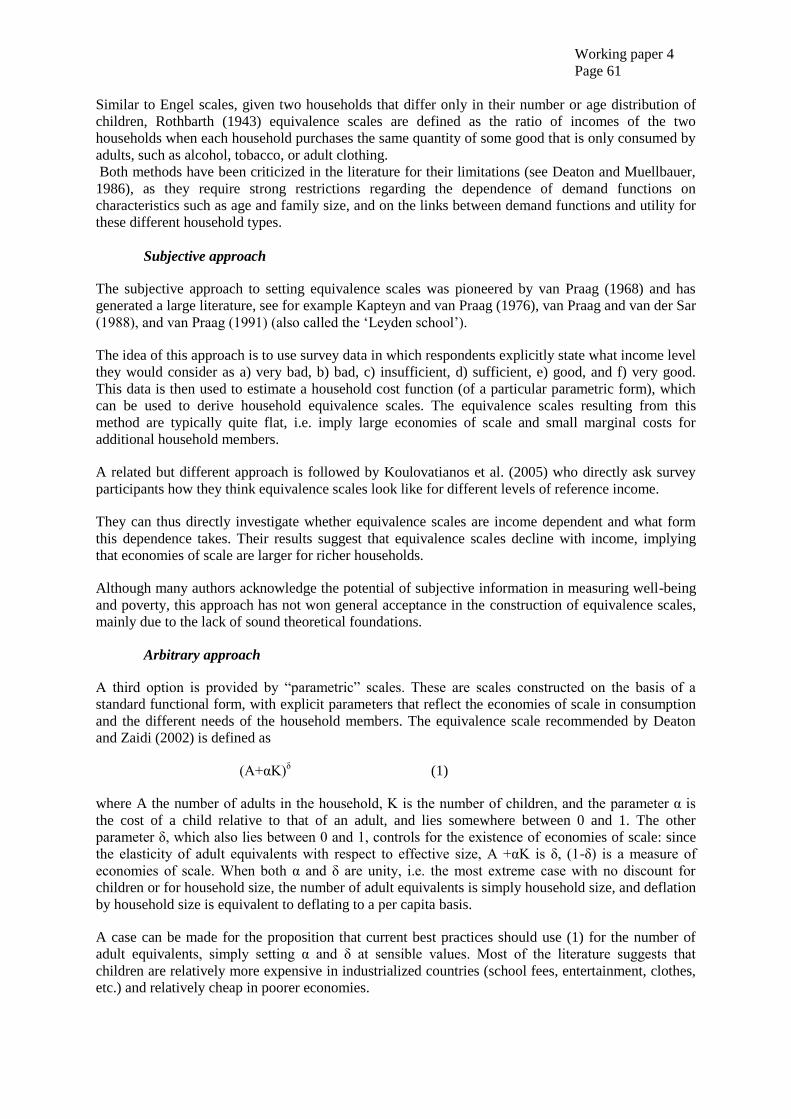
Working paper 4
Page 61
Similar to Engel scales, given two households that differ only in their number or age distribution of
children, Rothbarth (1943) equivalence scales are defined as the ratio of incomes of the two
households when each household purchases the same quantity of some good that is only consumed by
adults, such as alcohol, tobacco, or adult clothing.
Both methods have been criticized in the literature for their limitations (see Deaton and Muellbauer,
1986), as they require strong restrictions regarding the dependence of demand functions on
characteristics such as age and family size, and on the links between demand functions and utility for
these different household types.
Subjective approach
The subjective approach to setting equivalence scales was pioneered by van Praag (1968) and has
generated a large literature, see for example Kapteyn and van Praag (1976), van Praag and van der Sar
(1988), and van Praag (1991) (also called the ‘Leyden school’).
The idea of this approach is to use survey data in which respondents explicitly state what income level
they would consider as a) very bad, b) bad, c) insufficient, d) sufficient, e) good, and f) very good.
This data is then used to estimate a household cost function (of a particular parametric form), which
can be used to derive household equivalence scales. The equivalence scales resulting from this
method are typically quite flat, i.e. imply large economies of scale and small marginal costs for
additional household members.
A related but different approach is followed by Koulovatianos et al. (2005) who directly ask survey
participants how they think equivalence scales look like for different levels of reference income.
They can thus directly investigate whether equivalence scales are income dependent and what form
this dependence takes. Their results suggest that equivalence scales decline with income, implying
that economies of scale are larger for richer households.
Although many authors acknowledge the potential of subjective information in measuring well-being
and poverty, this approach has not won general acceptance in the construction of equivalence scales,
mainly due to the lack of sound theoretical foundations.
Arbitrary approach
A third option is provided by “parametric” scales. These are scales constructed on the basis of a
standard functional form, with explicit parameters that reflect the economies of scale in consumption
and the different needs of the household members. The equivalence scale recommended by Deaton
and Zaidi (2002) is defined as
(A+αK)δ
(1)
where A the number of adults in the household, K is the number of children, and the parameter α is
the cost of a child relative to that of an adult, and lies somewhere between 0 and 1. The other
parameter δ, which also lies between 0 and 1, controls for the existence of economies of scale: since
the elasticity of adult equivalents with respect to effective size, A +αK is δ, (1-δ) is a measure of
economies of scale. When both α and δ are unity, i.e. the most extreme case with no discount for
children or for household size, the number of adult equivalents is simply household size, and deflation
by household size is equivalent to deflating to a per capita basis.
A case can be made for the proposition that current best practices should use (1) for the number of
adult equivalents, simply setting α and δ at sensible values. Most of the literature suggests that
children are relatively more expensive in industrialized countries (school fees, entertainment, clothes,
etc.) and relatively cheap in poorer economies.
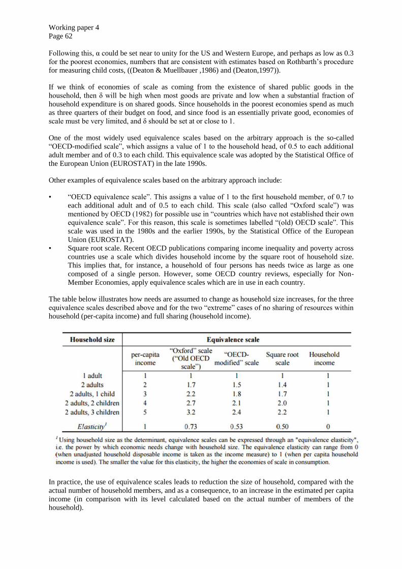
Working paper 4
Page 62
Following this, α could be set near to unity for the US and Western Europe, and perhaps as low as 0.3
for the poorest economies, numbers that are consistent with estimates based on Rothbarth’s procedure
for measuring child costs, ((Deaton & Muellbauer ,1986) and (Deaton,1997)).
If we think of economies of scale as coming from the existence of shared public goods in the
household, then δ will be high when most goods are private and low when a substantial fraction of
household expenditure is on shared goods. Since households in the poorest economies spend as much
as three quarters of their budget on food, and since food is an essentially private good, economies of
scale must be very limited, and δ should be set at or close to 1.
One of the most widely used equivalence scales based on the arbitrary approach is the so-called
“OECD-modified scale”, which assigns a value of 1 to the household head, of 0.5 to each additional
adult member and of 0.3 to each child. This equivalence scale was adopted by the Statistical Office of
the European Union (EUROSTAT) in the late 1990s.
Other examples of equivalence scales based on the arbitrary approach include:
• “OECD equivalence scale”. This assigns a value of 1 to the first household member, of 0.7 to
each additional adult and of 0.5 to each child. This scale (also called “Oxford scale”) was
mentioned by OECD (1982) for possible use in “countries which have not established their own
equivalence scale”. For this reason, this scale is sometimes labelled “(old) OECD scale”. This
scale was used in the 1980s and the earlier 1990s, by the Statistical Office of the European
Union (EUROSTAT).
• Square root scale. Recent OECD publications comparing income inequality and poverty across
countries use a scale which divides household income by the square root of household size.
This implies that, for instance, a household of four persons has needs twice as large as one
composed of a single person. However, some OECD country reviews, especially for Non-
Member Economies, apply equivalence scales which are in use in each country.
The table below illustrates how needs are assumed to change as household size increases, for the three
equivalence scales described above and for the two “extreme” cases of no sharing of resources within
household (per-capita income) and full sharing (household income).
In practice, the use of equivalence scales leads to reduction the size of household, compared with the
actual number of household members, and as a consequence, to an increase in the estimated per capita
income (in comparison with its level calculated based on the actual number of members of the
household).
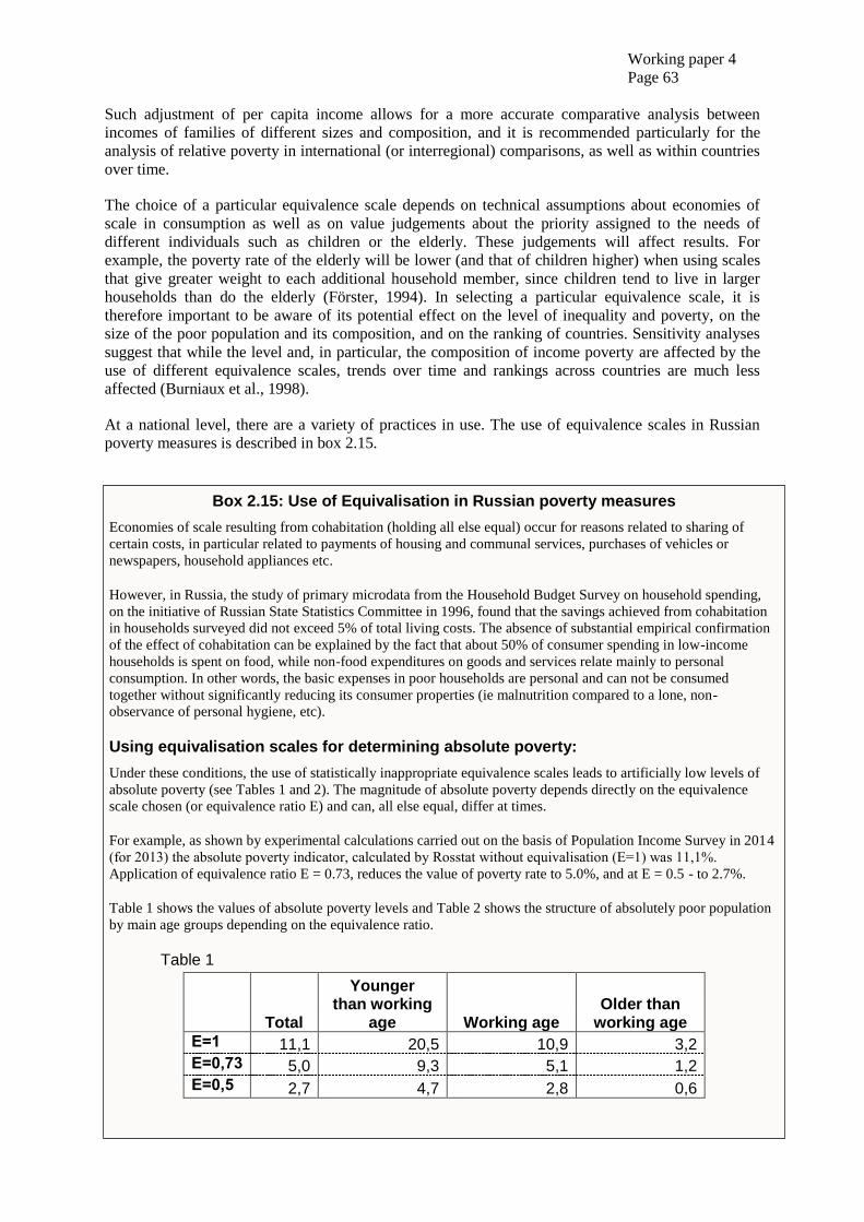
Working paper 4
Page 63
Such adjustment of per capita income allows for a more accurate comparative analysis between
incomes of families of different sizes and composition, and it is recommended particularly for the
analysis of relative poverty in international (or interregional) comparisons, as well as within countries
over time.
The choice of a particular equivalence scale depends on technical assumptions about economies of
scale in consumption as well as on value judgements about the priority assigned to the needs of
different individuals such as children or the elderly. These judgements will affect results. For
example, the poverty rate of the elderly will be lower (and that of children higher) when using scales
that give greater weight to each additional household member, since children tend to live in larger
households than do the elderly (Förster, 1994). In selecting a particular equivalence scale, it is
therefore important to be aware of its potential effect on the level of inequality and poverty, on the
size of the poor population and its composition, and on the ranking of countries. Sensitivity analyses
suggest that while the level and, in particular, the composition of income poverty are affected by the
use of different equivalence scales, trends over time and rankings across countries are much less
affected (Burniaux et al., 1998).
At a national level, there are a variety of practices in use. The use of equivalence scales in Russian
poverty measures is described in box 2.15.
Box 2.15: Use of Equivalisation in Russian poverty measures
Economies of scale resulting from cohabitation (holding all else equal) occur for reasons related to sharing of
certain costs, in particular related to payments of housing and communal services, purchases of vehicles or
newspapers, household appliances etc.
However, in Russia, the study of primary microdata from the Household Budget Survey on household spending,
on the initiative of Russian State Statistics Committee in 1996, found that the savings achieved from cohabitation
in households surveyed did not exceed 5% of total living costs. The absence of substantial empirical confirmation
of the effect of cohabitation can be explained by the fact that about 50% of consumer spending in low-income
households is spent on food, while non-food expenditures on goods and services relate mainly to personal
consumption. In other words, the basic expenses in poor households are personal and can not be consumed
together without significantly reducing its consumer properties (ie malnutrition compared to a lone, non-
observance of personal hygiene, etc).
Using equivalisation scales for determining absolute poverty:
Under these conditions, the use of statistically inappropriate equivalence scales leads to artificially low levels of
absolute poverty (see Tables 1 and 2). The magnitude of absolute poverty depends directly on the equivalence
scale chosen (or equivalence ratio E) and can, all else equal, differ at times.
For example, as shown by experimental calculations carried out on the basis of Population Income Survey in 2014
(for 2013) the absolute poverty indicator, calculated by Rosstat without equivalisation (Е=1) was 11,1%.
Application of equivalence ratio E = 0.73, reduces the value of poverty rate to 5.0%, and at E = 0.5 - to 2.7%.
Table 1 shows the values of absolute poverty levels and Table 2 shows the structure of absolutely poor population
by main age groups depending on the equivalence ratio.
Table 1
Total
Younger than working
age Working age Older than
working age
Е=1 11,1 20,5 10,9 3,2
Е=0,73 5,0 9,3 5,1 1,2
Е=0,5 2,7 4,7 2,8 0,6
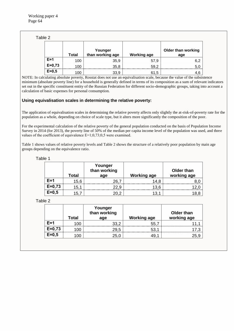
Working paper 4
Page 64
Table 2
Total Younger
than working age Working age Older than working
age
Е=1 100 35,9 57,9 6,2
Е=0,73 100 35,8 59,2 5,0
Е=0,5 100 33,9 61,5 4,6
NOTE: In calculating absolute poverty, Rosstat does not use an equivalisation scale, because the value of the subsistence
minimum (absolute poverty line) for a household is generally defined in terms of its composition as a sum of relevant indicators
set out in the specific constituent entity of the Russian Federation for different socio-demographic groups, taking into account a
calculation of basic expenses for personal consumption.
Using equivalisation scales in determining the relative poverty:
The application of equivalisation scales in determining the relative poverty affects only slightly the at-risk-of-poverty rate for the
population as a whole, depending on choice of scale type, but it alters more significantly the composition of the poor.
For the experimental calculation of the relative poverty of the general population conducted on the basis of Population Income
Survey in 2014 (for 2013), the poverty line of 50% of the median per capita income level of the population was used, and three
values of the coefficient of equivalence Е=1;0,73;0,5 were examined.
Table 1 shows values of relative poverty levels and Table 2 shows the structure of a relatively poor population by main age
groups depending on the equivalence ratio.
Table 1
Total
Younger than working
age Working age Older than
working age
Е=1 15,6 26,7 14,8 8,0
Е=0,73 15,1 22,9 13,6 12,0
Е=0,5 15,7 20,2 13,1 18,8
Table 2
Total
Younger than working
age Working age Older than
working age
Е=1 100 33,2 55,7 11,1
Е=0,73 100 29,5 53,1 17,3
Е=0,5 100 25,0 49,1 25,9
Working paper 4
Page 65
b. Prices and PPPs; International Comparison Program (ICP)
Cross-country comparisons of poverty rates crucially depend on the information about the level of
prices in various countries, except where fully relative measures of poverty are used. This information
plays an essential role because it enables researchers to compare welfare between individuals living in
different countries, by adjusting domestic incomes by PPP (purchasing power parity) exchange rates,
so that one international dollar provides, in principle, the same command over goods and services in
any country of the world.2 PPP exchange rates play a role similar to that played by national price
indexes in the case of individual countries over time. In order to compare average or individual
welfare in the same country in two periods of time, one needs to adjust for changing national price
level. Similarly, to compare welfare between individuals living in different countries at the same point
in time, one needs an estimate of price levels they face. Cross-country comparisons of poverty rates
are thus sensitive to the estimates of PPP exchange rates.
These estimates are obtained through a large International Comparison Program (ICP).3 The ICP is a
joint UN-OECD-World Bank-regional development Bank project that, at approximately decennial
intervals, has the objective of determining, from direct price comparisons of about 1000 goods and
services, price levels within nations, thus allowing to construct country-wide price indexes for total
GDP and various components of GDP such as household consumption, investment or government
spending and even narrower components of expenditures like clothing and footwear, transport, etc.
PPPs are calculated in several stages: first for individual goods and services, then for groups of
products, and finally for each of the various levels of aggregation up to GDP. PPPs continue to be
price relatives whether they refer to a product group, to an aggregation level, or to GDP. In moving up
the aggregation hierarchy, the price relatives refer to increasingly complex assortments of goods and
services. Thus, if the PPP for GDP between France and the United States is €0.95 to the dollar, it can
be inferred that for every dollar spent on GDP in the United States, €0.95 would have to be spent in
France to purchase the same volume of goods and services.
Purchasing the same volume of goods and services does not mean that the baskets of goods and
services purchased in both economies will be identical. The composition of the baskets will vary
between economies and reflect differences in tastes, cultures, climates, price structures, product
availability, and income levels, but both baskets will, in principle, provide equivalent satisfaction or
utility. PPP indexes are further standardised by expressing them in a common currency unit. The
common currency used for the global comparison is the US dollar, and so each economy’s PPP is
standardised by dividing it by that economy’s dollar exchange rate. The standardised indexes so
obtained are called price level indexes (PLIs or $PPP).4
Since the early 1990s, the World Bank has monitored global extreme poverty using an international
poverty line that was explicitly based upon the national poverty lines of some of the poorest countries
in the world. Each release of new PPP data has led both to revisions of the international poverty line,
and to re-assessments of the relative differences in well-being across countries and regions.
To measure poverty in different countries using these international poverty lines, the following three
steps are undertaken. First, the international poverty line is turned into a poverty line in national
2 For example, if the price of a hamburger in France is €4.80 and in the United States it is $4.00, the PPP for hamburgers between the two
economies is $0.83 to the euro from the French perspective (4.00/4.80) and €1.20 to the dollar from the U.S. perspective (4.80/4.00). In other words, for every euro spent on hamburgers in France, $0.83 would have to be spent in the United States to obtain the same quantity
and quality—that is, the same volume—of hamburgers. Conversely, for every dollar spent on hamburgers in the United States, €1.20 would
have to be spent in France to obtain the same volume of hamburgers. To compare the volumes of hamburgers purchased in the two economies, either the expenditure on hamburgers in France can be expressed in dollars by dividing by 1.20 or the expenditure on
hamburgers in the United States can be expressed in euros by dividing by 0.83. 3 For more details on the ICP, see http://go.worldbank.org/X3R0INNH80. 4 Economies with PLIs greater than 100 have price levels that are higher than that of the base economy. Economies with PLIs less than 100
have price levels that are lower than that of the base economy. So, returning to the hamburger example, if the exchange rate is $1.00 to
€0.79, the PLI for a hamburger with the United States as the base economy is 152 (1.20/0.79 × 100). From this, it can be inferred that, given the relative purchasing power of the dollar and the euro, hamburgers cost 52 percent more in France than they do in the United States.
Working paper 4
Page 66
currencies at the benchmark year using the PPP exchange rates from the particular ICP round. Second,
this poverty line is adjusted using national inflation rates to generate poverty lines in national
currencies backwards and forward in time. Third, the share of the population living below this poverty
line is then determined using national household income or expenditure surveys. It is important to
emphasise that, in each revision, poverty rates are recalculated not only for the most recent years, but
for all years since the beginning of measurement of poverty at the global level (where the first data
point generally produced is 1981).
The first international poverty line that was based on a sample of national poverty lines was set at
$1.01 using 1985 PPPs, by Ravallion, Datt and van de Walle (1991) and used in the 1990 World
Development Report (World Bank, 1990). Chen and Ravallion (2001) later updated this to $1.08 per
day, using the 1993 PPPs. With the release of the 2005 PPPs and a new set of national poverty lines,
Ravallion, Chen and Sangraula (2009) proposed a new global poverty line of $1.25 per day.
The latest round of ICP was conducted in 2011, and in October 2014 the full set of final results was
presented to the public. The new estimates of price levels in 199 countries led to the new estimates of
PPP exchange rates, and accordingly new $PPP estimates of national aggregates for all the
participating countries. Though there was some disagreement among scholars, the dominant view is
that these new PPPs represented an improvement over the 2005 set, creating the need for another
revision to the World Bank’s international poverty line.
In 2015 the World Bank revised its international poverty line by taking the national poverty lines for
15 very poor countries (expressed in local currency units at 2005 prices), and inflating them to 2011
using each country’s own consumer price index. Then, once in 2011 prices, these national lines were
converted into the US dollar using the 2011 PPPs, and a simple average were taken. The result of
those operations yielded $1.88 per person per day, which the World Bank rounded up to $1.90, and
which represent the new World Bank’s international poverty line.
It is important to note that PPPs offer comparisons across economies, not across the rich and poor
within economies. This may turn out to be problematic, since the spending patterns of poor
households differ systematically from those of the better-off. The poor spend a large proportion –
often a majority – of their incomes on basic staple foods, which account for a relatively small
proportion of the spending of the better-off, and therefore of the country as a whole.
To address this shortcoming, research was carried out by Deaton and Dupriez (2011), where they used
household surveys from 62 developing countries to calculate global poverty-weighted PPPs and to
calculate global poverty lines and new global poverty counts. They noted though that their research
did not attempt to use separate prices for the poor. Instead, they reweighted the same ICP-collected
prices to match the expenditure patterns of households near the global poverty line.
Another research was conducted by the Asian Development Bank (2008) to examine whether the
prices collected under the ICP are appropriate for poverty uses, using data from the ICP 2005 for 16
Asian countries.
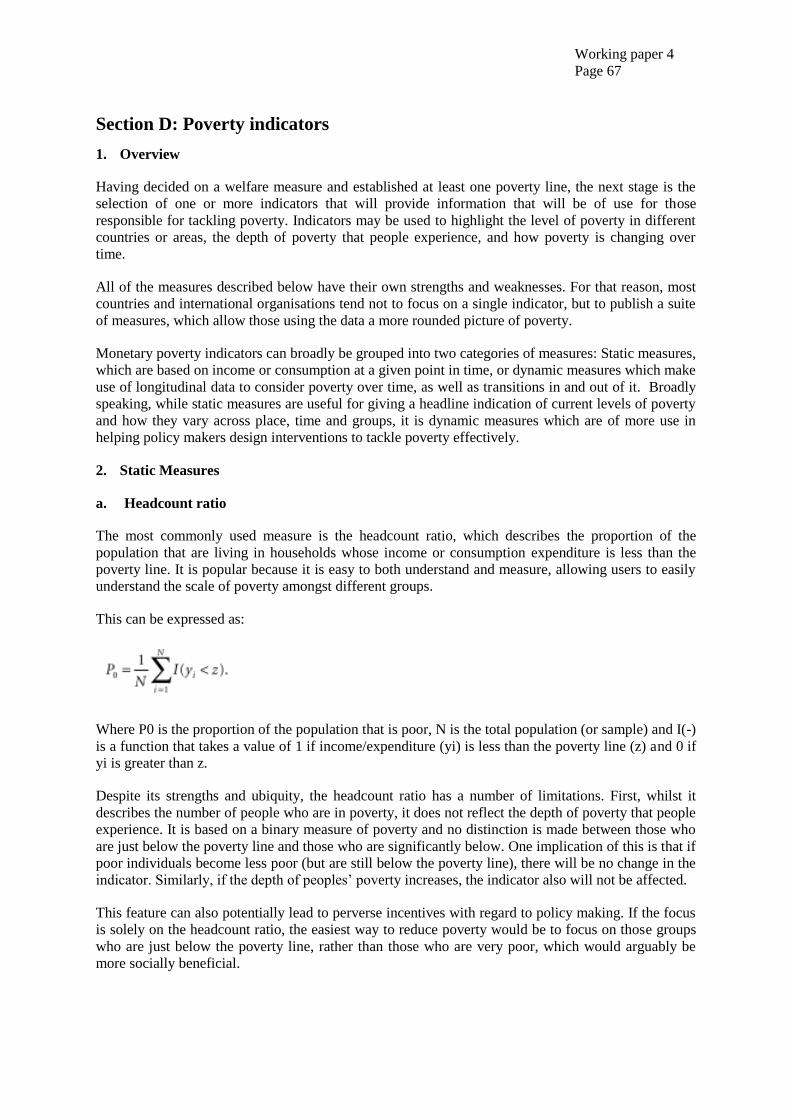
Working paper 4
Page 67
Section D: Poverty indicators
1. Overview
Having decided on a welfare measure and established at least one poverty line, the next stage is the
selection of one or more indicators that will provide information that will be of use for those
responsible for tackling poverty. Indicators may be used to highlight the level of poverty in different
countries or areas, the depth of poverty that people experience, and how poverty is changing over
time.
All of the measures described below have their own strengths and weaknesses. For that reason, most
countries and international organisations tend not to focus on a single indicator, but to publish a suite
of measures, which allow those using the data a more rounded picture of poverty.
Monetary poverty indicators can broadly be grouped into two categories of measures: Static measures,
which are based on income or consumption at a given point in time, or dynamic measures which make
use of longitudinal data to consider poverty over time, as well as transitions in and out of it. Broadly
speaking, while static measures are useful for giving a headline indication of current levels of poverty
and how they vary across place, time and groups, it is dynamic measures which are of more use in
helping policy makers design interventions to tackle poverty effectively.
2. Static Measures
a. Headcount ratio
The most commonly used measure is the headcount ratio, which describes the proportion of the
population that are living in households whose income or consumption expenditure is less than the
poverty line. It is popular because it is easy to both understand and measure, allowing users to easily
understand the scale of poverty amongst different groups.
This can be expressed as:
Where P0 is the proportion of the population that is poor, N is the total population (or sample) and I(-)
is a function that takes a value of 1 if income/expenditure (yi) is less than the poverty line (z) and 0 if
yi is greater than z.
Despite its strengths and ubiquity, the headcount ratio has a number of limitations. First, whilst it
describes the number of people who are in poverty, it does not reflect the depth of poverty that people
experience. It is based on a binary measure of poverty and no distinction is made between those who
are just below the poverty line and those who are significantly below. One implication of this is that if
poor individuals become less poor (but are still below the poverty line), there will be no change in the
indicator. Similarly, if the depth of peoples’ poverty increases, the indicator also will not be affected.
This feature can also potentially lead to perverse incentives with regard to policy making. If the focus
is solely on the headcount ratio, the easiest way to reduce poverty would be to focus on those groups
who are just below the poverty line, rather than those who are very poor, which would arguably be
more socially beneficial.
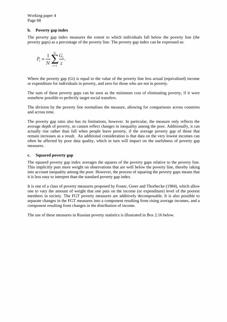
Working paper 4
Page 68
b. Poverty gap index
The poverty gap index measures the extent to which individuals fall below the poverty line (the
poverty gaps) as a percentage of the poverty line. The poverty gap index can be expressed as:
Where the poverty gap (Gi) is equal to the value of the poverty line less actual (equivalised) income
or expenditure for individuals in poverty, and zero for those who are not in poverty.
The sum of these poverty gaps can be seen as the minimum cost of eliminating poverty, if it were
somehow possible to perfectly target social transfers.
The division by the poverty line normalises the measure, allowing for comparisons across countries
and across time.
The poverty gap ratio also has its limitations, however. In particular, the measure only reflects the
average depth of poverty, so cannot reflect changes in inequality among the poor. Additionally, it can
actually rise rather than fall when people leave poverty, if the average poverty gap of those that
remain increases as a result. An additional consideration is that data on the very lowest incomes can
often be affected by poor data quality, which in turn will impact on the usefulness of poverty gap
measures.
c. Squared poverty gap
The squared poverty gap index averages the squares of the poverty gaps relative to the poverty line.
This implicitly puts more weight on observations that are well below the poverty line, thereby taking
into account inequality among the poor. However, the process of squaring the poverty gaps means that
it is less easy to interpret than the standard poverty gap index.
It is one of a class of poverty measures proposed by Foster, Greer and Thorbecke (1984), which allow
one to vary the amount of weight that one puts on the income (or expenditure) level of the poorest
members in society. The FGT poverty measures are additively decomposable. It is also possible to
separate changes in the FGT measures into a component resulting from rising average incomes, and a
component resulting from changes in the distribution of income.
The use of these measures in Russian poverty statistics is illustrated in Box 2.16 below.
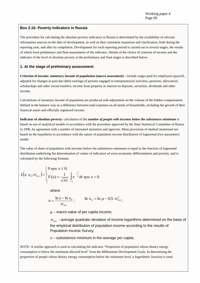
Working paper 4
Page 69
Box 2.16: Poverty indicators in Russia
The procedure for calculating the absolute poverty indicators in Russia is determined by the availability of relevant
information sources on the date of development, as well as their consistent expansion and clarification, both during the
reporting year, and after its completion. Development for each reporting period is carried out in several stages, the results
of which form preliminary and final assessments of the indicator. Details of the choice of criterion of income and the
indicator of the level of absolute poverty at the preliminary and final stages is described below:
1. At the stage of preliminary assessment:
Criterion of income: monetary income of population (macro assessment) - include wages paid for employees (payroll,
adjusted for changes in past-due debt) earnings of persons engaged in entrepreneurial activities, pensions, allowances,
scholarships and other social transfers, income from property as interest on deposits, securities, dividends and other
income.
Calculations of monetary income of population are produced with adjustment on the volume of the hidden compensation
defined in the balance way as a difference between total expenses on all needs of households, including the growth of their
financial assets and officially registered income.
Indicator of absolute poverty: calculation of the number of people with incomes below the subsistence minimum is
based on use of analytical models in accordance with the procedure approved by the State Statistical Committee of Russia
in 1996, by agreement with a number of interested ministries and agencies. Main provisions of method mentioned are
based on the hypothesis in accordance with the nature of population income distribution of lognormal (two-parameter)
model.
The value of share of population with incomes below the subsistence minimum is equal to the function of lognormal
distribution underlying the determination of values of indicators of socio-economic differentiation and poverty, and is
calculated by the following formula:
.02
1)(
;00
;;2ln0
2
xприdteuF
xпри
xzLu t
x
where
x
xzu
ln
0lnln
;
2
xln0 5,0lnxln ;
μ – macro-value of per capita income;
xln - average quadratic deviation of income logarithms determined on the basis of
the empirical distribution of population income according to the results of
Population Income Survey;
z – subsistence minimum in the average per capita.
NOTE: A similar approach is used in calculating the indicator "Proportion of population whose dietary energy
consumption is below the minimum allowed level" from the Millennium Development Goals. In determining the
proportion of people whose dietary energy consumption below the minimum level, a logarithmic function is used.
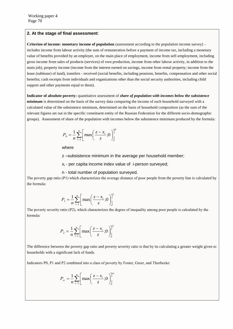
Working paper 4
Page 70
2. At the stage of final assessment:
Criterion of income: monetary income of population (assessment according to the population income survey) –
includes income from labour activity (the sum of remuneration before a payment of income tax, including a monetary
value of benefits provided by an employer, on the main place of employment, income from self-employment, including
gross income from sales of products (services) of own production, income from other labour activity, in addition to the
main job), property income (income from the interest earned on savings, income from rental property; income from the
lease (sublease) of land), transfers - received (social benefits, including pensions, benefits, compensation and other social
benefits; cash receipts from individuals and organizations other than the social security authorities, including child
support and other payments equal to them).
Indicator of absolute poverty: quantitative assessment of share of population with incomes below the subsistence
minimum is determined on the basis of the survey data comparing the income of each household surveyed with a
calculated value of the subsistence minimum, determined on the basis of household composition (as the sum of the
relevant figures set out in the specific constituent entity of the Russian Federation for the different socio-demographic
groups). Assessment of share of the population with incomes below the subsistence minimum produced by the formula:
n
i
i
z
xz
nР
1
0
0 0;max1
where
z –subsistence minimum in the average per household member;
xi - per capita income index value of i-person surveyed;
n - total number of population surveyed.
The poverty gap ratio (Р1) which characterizes the average distance of poor people from the poverty line is calculated by
the formula:
n
i
i
z
xz
nР
1
1
1 0;max1
The poverty severity ratio (Р2), which characterizes the degree of inequality among poor people is calculated by the
formula:
n
i
i
z
xz
nР
1
2
2 0;max1
The difference between the poverty gap ratio and poverty severity ratio is that by its calculating a greater weight given to
households with a significant lack of funds.
Indicators Р0, Р1 and Р2 combined into a class of poverty by Foster, Greer, and Thorbecke:
n
i
i
z
xz
nР
1
0;max1
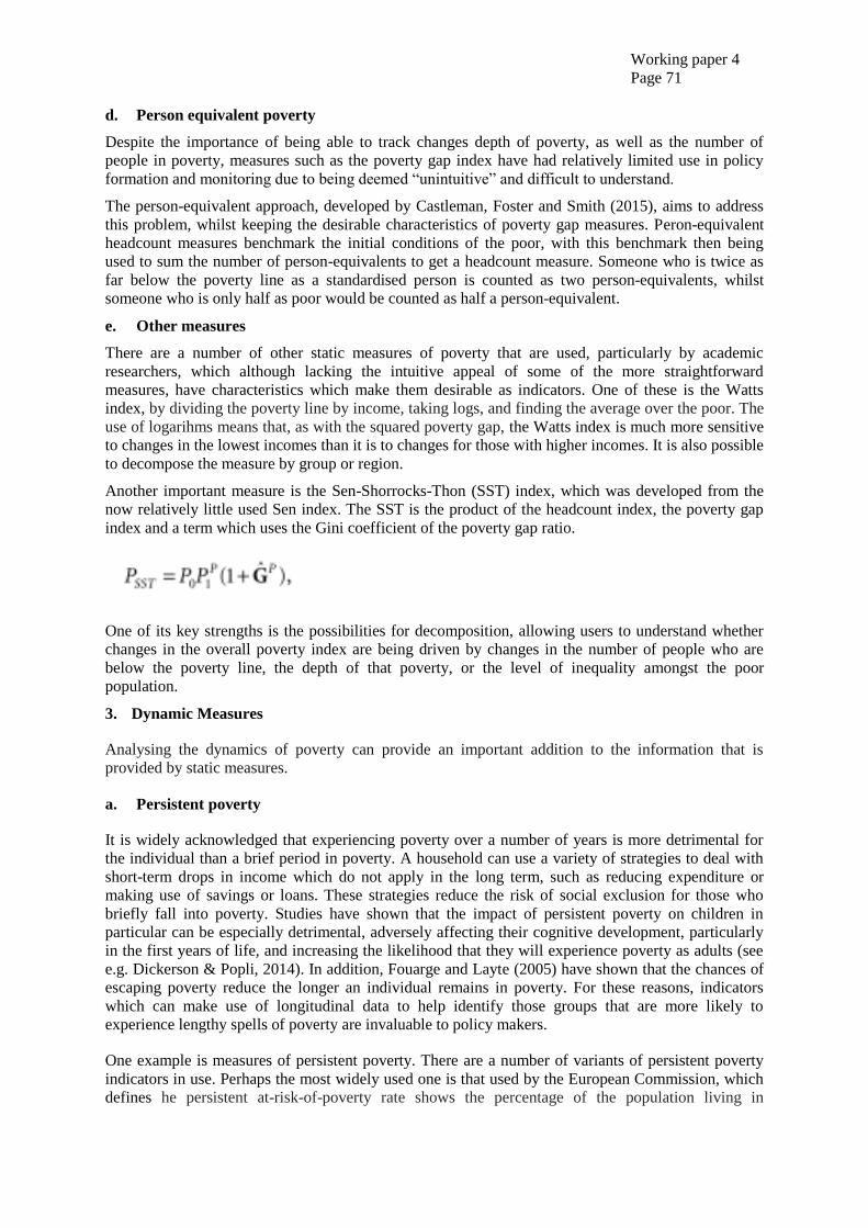
Working paper 4
Page 71
d. Person equivalent poverty
Despite the importance of being able to track changes depth of poverty, as well as the number of
people in poverty, measures such as the poverty gap index have had relatively limited use in policy
formation and monitoring due to being deemed “unintuitive” and difficult to understand.
The person-equivalent approach, developed by Castleman, Foster and Smith (2015), aims to address
this problem, whilst keeping the desirable characteristics of poverty gap measures. Peron-equivalent
headcount measures benchmark the initial conditions of the poor, with this benchmark then being
used to sum the number of person-equivalents to get a headcount measure. Someone who is twice as
far below the poverty line as a standardised person is counted as two person-equivalents, whilst
someone who is only half as poor would be counted as half a person-equivalent.
e. Other measures
There are a number of other static measures of poverty that are used, particularly by academic
researchers, which although lacking the intuitive appeal of some of the more straightforward
measures, have characteristics which make them desirable as indicators. One of these is the Watts
index, by dividing the poverty line by income, taking logs, and finding the average over the poor. The
use of logarihms means that, as with the squared poverty gap, the Watts index is much more sensitive
to changes in the lowest incomes than it is to changes for those with higher incomes. It is also possible
to decompose the measure by group or region.
Another important measure is the Sen-Shorrocks-Thon (SST) index, which was developed from the
now relatively little used Sen index. The SST is the product of the headcount index, the poverty gap
index and a term which uses the Gini coefficient of the poverty gap ratio.
One of its key strengths is the possibilities for decomposition, allowing users to understand whether
changes in the overall poverty index are being driven by changes in the number of people who are
below the poverty line, the depth of that poverty, or the level of inequality amongst the poor
population.
3. Dynamic Measures
Analysing the dynamics of poverty can provide an important addition to the information that is
provided by static measures.
a. Persistent poverty
It is widely acknowledged that experiencing poverty over a number of years is more detrimental for
the individual than a brief period in poverty. A household can use a variety of strategies to deal with
short-term drops in income which do not apply in the long term, such as reducing expenditure or
making use of savings or loans. These strategies reduce the risk of social exclusion for those who
briefly fall into poverty. Studies have shown that the impact of persistent poverty on children in
particular can be especially detrimental, adversely affecting their cognitive development, particularly
in the first years of life, and increasing the likelihood that they will experience poverty as adults (see
e.g. Dickerson & Popli, 2014). In addition, Fouarge and Layte (2005) have shown that the chances of
escaping poverty reduce the longer an individual remains in poverty. For these reasons, indicators
which can make use of longitudinal data to help identify those groups that are more likely to
experience lengthy spells of poverty are invaluable to policy makers.
One example is measures of persistent poverty. There are a number of variants of persistent poverty
indicators in use. Perhaps the most widely used one is that used by the European Commission, which
defines he persistent at-risk-of-poverty rate shows the percentage of the population living in
Working paper 4
Page 72
households where the equivalised disposable income was below the at-risk-of-poverty threshold for
the current year and at least two out of the preceding three years. Its calculation requires a
longitudinal instrument, through which the individuals are followed over four years.
Box 2.17 provides examples of the analysis of both the persistent at-risk-of-poverty rate and entry and
exit rates in the UK and other EU countries
b. Entry and exit rates
Another important application of longitudinal data is to examine transitions in and out of poverty
between one year and the next. This can be particularly useful where limited panel durations make
analysis of poverty spell length challenging.
The entry rate into poverty is generally measured as the percentage of people who were not in poverty
one year earlier but fell into poverty in the following year. Conversely, the exit rate is defined as the
percentage of individuals not at-risk-of-poverty in the current year among those who were at-risk-of-
poverty the year before.
To note that because there are fewer people in poverty than not in poverty, it is to be expected that
exit rates expressed as a percentage of those in poverty will almost always5 be higher than entry rates
as a percentage of those not in poverty; small changes in the number of people in each case would
equate to a much larger percentage change for those in poverty.
Box 2.18 provides an example of analysis of poverty entry and exit rates conducted by the European
Commission.
5 This is true where there are more people out of poverty than in. This may not be the case for all groups,
concepts or countries.
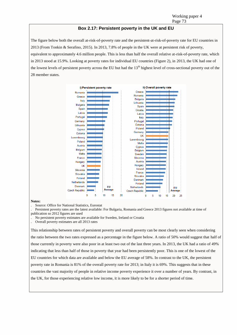
Working paper 4
Page 73
Box 2.17: Persistent poverty in the UK and EU
The figure below both the overall at-risk-of-poverty rate and the persistent-at-risk-of-poverty rate for EU countries in
2013 (From Tonkin & Serafino, 2015). In 2013, 7.8% of people in the UK were at persistent risk of poverty,
equivalent to approximately 4.6 million people. This is less than half the overall relative at-risk-of-poverty rate, which
in 2013 stood at 15.9%. Looking at poverty rates for individual EU countries (Figure 2), in 2013, the UK had one of
the lowest levels of persistent poverty across the EU but had the 13th
highest level of cross-sectional poverty out of the
28 member states.
Notes:
. Source: Office for National Statistics, Eurostat
. Persistent poverty rates are the latest available: For Bulgaria, Romania and Greece 2013 figures not available at time of
publication so 2012 figures are used
. No persistent poverty estimates are available for Sweden, Ireland or Croatia
. Overall poverty estimates are all 2013 rates
This relationship between rates of persistent poverty and overall poverty can be most clearly seen when considering
the ratio between the two rates expressed as a percentage in the figure below. A ratio of 50% would suggest that half of
those currently in poverty were also poor in at least two out of the last three years. In 2013, the UK had a ratio of 49%
indicating that less than half of those in poverty that year had been persistently poor. This is one of the lowest of the
EU countries for which data are available and below the EU average of 58%. In contrast to the UK, the persistent
poverty rate in Romania is 81% of the overall poverty rate for 2013; in Italy it is 69%. This suggests that in these
countries the vast majority of people in relative income poverty experience it over a number of years. By contrast, in
the UK, for those experiencing relative low income, it is more likely to be for a shorter period of time.
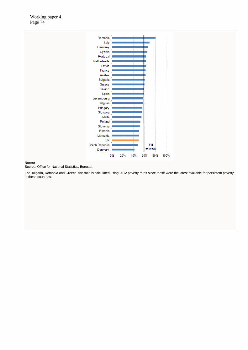
Working paper 4
Page 74
Notes: Source: Office for National Statistics, Eurostat
For Bulgaria, Romania and Greece, the ratio is calculated using 2012 poverty rates since these were the latest available for persistent poverty in these countries.
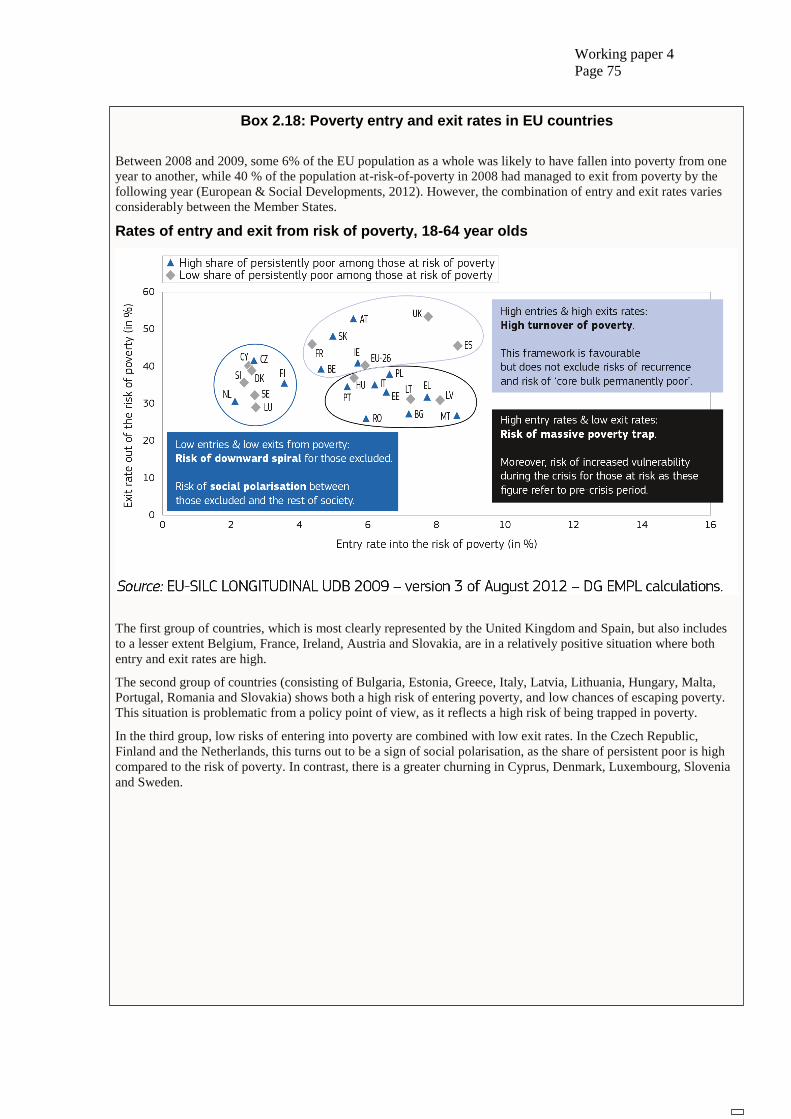
Working paper 4
Page 75
Box 2.18: Poverty entry and exit rates in EU countries
Between 2008 and 2009, some 6% of the EU population as a whole was likely to have fallen into poverty from one
year to another, while 40 % of the population at-risk-of-poverty in 2008 had managed to exit from poverty by the
following year (European & Social Developments, 2012). However, the combination of entry and exit rates varies
considerably between the Member States.
Rates of entry and exit from risk of poverty, 18-64 year olds
The first group of countries, which is most clearly represented by the United Kingdom and Spain, but also includes
to a lesser extent Belgium, France, Ireland, Austria and Slovakia, are in a relatively positive situation where both
entry and exit rates are high.
The second group of countries (consisting of Bulgaria, Estonia, Greece, Italy, Latvia, Lithuania, Hungary, Malta,
Portugal, Romania and Slovakia) shows both a high risk of entering poverty, and low chances of escaping poverty.
This situation is problematic from a policy point of view, as it reflects a high risk of being trapped in poverty.
In the third group, low risks of entering into poverty are combined with low exit rates. In the Czech Republic,
Finland and the Netherlands, this turns out to be a sign of social polarisation, as the share of persistent poor is high
compared to the risk of poverty. In contrast, there is a greater churning in Cyprus, Denmark, Luxembourg, Slovenia
and Sweden.
Working paper 4
Page 76
Section E: Review of Current Practices
1. Review of national practices
[TO BE DEVELOPED]
2. Comparability of Poverty Estimates
International comparability of poverty estimates has improved in recent decades. However, there is no
universal approach to poverty measurement that would fit all countries.
a. MDGs and their impact on poverty comparability
The MDG indicators on poverty were not fully suitable for comparing poverty in the UNECE region.
About half of the UNECE countries are middle and higher income countries, where physical survival
is generally given, the majority of the poor live above $1 per day, and many of the MDG indicators
are of limited relevance for their stage of development. Surveys needed for the estimation of some of
the internationally agreed upon indicators are not always conducted in these countries. They have in
place and continue to use alternative indicators that are more relevant to them and their national
policies.
Nevertheless, thanks to the MDGs, the low-income countries made a big and important step towards
comparability of poverty estimates, often based on indicators available from surveys conducted in
such countries under the supervision of United Nations and other international organizations.
Imperfect as it might be, the “$1-a-day” poverty line has been adopted as one the main official
indicators for monitoring progress towards the First Millennium Development Goal, aimed at
eradicating extreme poverty and hunger by 2015. In particular, the first target (1.A) explicitly points
towards “halving the proportion of people whose in-come is less than one dollar a day” with respect to
1990. To better fit countries' needs, the internationally-comparable absolute poverty lines have been
amended to $1.00, $1.25 or $2.50 per day. The need to use a universal poverty line as indicator was
reaffirmed with the recently adopted new global Sustainable Development Goals6. Goal 1: “End
poverty in all its forms everywhere”, first target (1.1) states: “By 2030, eradicate extreme poverty for
all people everywhere, currently measured as people living on less than $1.25 a day”.
Figure 3 is based on data from official reports and databases on UNECE countries reporting on
MDGs. It shows that the majority of the countries are using international approaches when publishing
official estimates for MDG reporting. In the few occasions when both national and international
approaches are used, one can usually see a difference in the results. Despite these discrepancies, the
work on calculation of internationally comparable estimates has made a significant progress.
6 https://sustainabledevelopment.un.org/
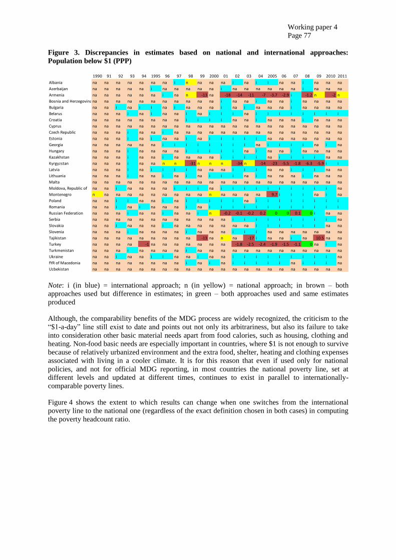
Working paper 4
Page 77
Figure 3. Discrepancies in estimates based on national and international approaches:
Population below $1 (PPP)
Note: i (in blue) = international approach; n (in yellow) = national approach; in brown – both
approaches used but difference in estimates; in green – both approaches used and same estimates
produced
Although, the comparability benefits of the MDG process are widely recognized, the criticism to the
“$1-a-day” line still exist to date and points out not only its arbitrariness, but also its failure to take
into consideration other basic material needs apart from food calories, such as housing, clothing and
heating. Non-food basic needs are especially important in countries, where $1 is not enough to survive
because of relatively urbanized environment and the extra food, shelter, heating and clothing expenses
associated with living in a cooler climate. It is for this reason that even if used only for national
policies, and not for official MDG reporting, in most countries the national poverty line, set at
different levels and updated at different times, continues to exist in parallel to internationally-
comparable poverty lines.
Figure 4 shows the extent to which results can change when one switches from the international
poverty line to the national one (regardless of the exact definition chosen in both cases) in computing
the poverty headcount ratio.
1990 91 92 93 94 1995 96 97 98 99 2000 01 02 03 04 2005 06 07 08 09 2010 2011
Albania na na na na na na na i n na na na i na i i na na i na na na
Azerbaijan na na na na na i na na na na na i na na na na na na i na na na
Armenia na na na na na na i na n -13 na -18 -14 -11 -7 -3.7 -2.9 i -1.2 n -2 n
Bosnia and Herzegovina na na na na na na na na na na na i na na i na na i na na na na
Bulgaria na na i na i i na i na na na i na i na na na i na na na na
Belarus na na na i na i na na i na i i i na i i i i i i i i
Croatia na na na na na na na na i i i i na na i na na na i na na na
Cyprus na na na na na na na na na na na na na na na na na na na na na na
Czech Republic na na na i na na i na na na na na na na na na na na na na na na
Estonia na na na i na i na na i na i i i i i na na na na na na na
Georgia na na na na na na i i i i i i i i na i i i i na i na
Hungary na na na i na na na na i i i i i na i na na i na na na na
Kazakhstan na na na i na na i na na na na i i i i na i i i i na na
Kyrgyzstan na na na i na na n n -31 n n n -34 n -14 -23 -5.5 -1.8 -6.3 -5.9 i i
Latvia na na na i na i i i i na na na i i i na na i i i na na
Lithuania na na na i na na i na i na i i i na i na na na i na na na
Malta na na na na na na na na na na na na na na na na na na na na na na
Moldova, Republic of na na i na na na na i i i na i i i i i i i i i i na
Montenegro n na na na na na na na na na n na na na na 9.7 i i i na i na
Poland na na i i na na i na i i i i i na i i i i i i i i
Romania na na i na i na na na i na i i i i i i i i i i i i
Russian Federation na na na i na na i na na i n -0.2 -0.1 -0.2 0.2 0 0 0.1 0 i na na
Serbia na na na na na na na na na na na na i i i i i i i i i na
Slovakia na na i na na na i na na na na na na na i i i i i i na na
Slovenia na na na i na na na na i na na na i i i na na na na na na na
Tajikistan na na na na na na na na na -13 na n na -17 i na na i na 10.5 na na
Turkey na na na na -1 na na na na na na na -1.8 -2.5 -2.4 -1.9 -1.5 -1.1 0 na i na
Turkmenistan na na na i na na na na i na na na na na na na na na na na na na
Ukraine na na i na na i i na na i na na i i i i i i i i i na
fYR of Macedonia na na na na na na na na i na i na i i i i i na i i i na
Uzbekistan na na na na na na na na na na na na na na na na na na na na na na
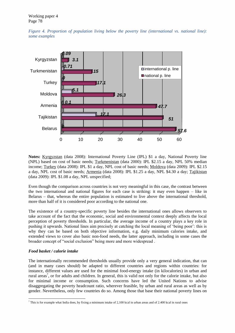
Working paper 4
Page 78
Figure 4. Proportion of population living below the poverty line (international vs. national line):
some examples
Notes: Kyrgyzstan (data 2008): International Poverty Line (IPL) $1 a day, National Poverty line
(NPL) based on cost of basic needs; Turkmenistan (data 2000): IPL $2.15 a day, NPL 50% median
income; Turkey (data 2008): IPL $1 a day, NPL cost of basic needs; Moldova (data 2009): IPL $2.15
a day, NPL cost of basic needs; Armenia (data 2008): IPL $1.25 a day, NPL $4.30 a day; Tajikistan
(data 2009): IPL $1.08 a day, NPL unspecified;
Even though the comparison across countries is not very meaningful in this case, the contrast between
the two international and national figures for each case is striking: it may even happen – like in
Belarus – that, whereas the entire population is estimated to live above the international threshold,
more than half of it is considered poor according to the national one.
The existence of a country-specific poverty line besides the international ones allows observers to
take account of the fact that the economic, social and environmental context deeply affects the local
perception of poverty thresholds. In particular, the average income of a country plays a key role in
pushing it upwards. National lines aim precisely at catching the local meaning of ‘being poor’: this is
why they can be based on both objective information, e.g. daily minimum calories intake, and
extended views to cover also basic non-food needs, the latter approach, including in some cases the
broader concept of “social exclusion” being more and more widespread .
Food basket / calorie intake
The internationally recommended thresholds usually provide only a very general indication, that can
(and in many cases should) be adapted to different countries and regions within countries: for
instance, different values are used for the minimal food-energy intake (in kilocalories) in urban and
rural areas7, or for adults and children. In general, this is valid not only for the calorie intake, but also
for minimal income or consumption. Such concerns have led the United Nations to advise
disaggregating the poverty headcount ratio, wherever feasible, by urban and rural areas as well as by
gender. Nevertheless, only few countries do so. Among those that base their national poverty lines on
7 This is for example what India does, by fixing a minimum intake of 2,100 kcal in urban areas and of 2.400 kcal in rural ones
0 10 20 30 40 50 60
Belarus
Tajikistan
Armenia
Moldova
Turkey
Turkmenistan
Kyrgyzstan
57.6
51
47.7
26.3
17.1
15
3.1
0
17.1
0.1
5.1
0
0.71
0.09
international p. line
national p. line
Working paper 4
Page 79
a food basket, only Kazakhstan, Kyrgyzstan and Uzbekistan distinguish between towns and
countryside, whereas only Uzbekistan presents data separated by sex. One should consider, however,
that in order to disaggregate by gender, it is necessary either to record and analyse data on an
individual (rather than household) basis, which is quite rare and expensive, or to refer to the gender of
the household head.
Basic non-food needs / Social exclusion
Many countries use, in addition to the food-basket based indicator, also another, less strict one, for
gauging less severe poverty. This latter index is usually named as national poverty line according to
basic needs, and refers to the income required to purchase (or the consumption level corresponding
to) essential amounts of food, clothes, heating, and housing availability. According to the World
Bank, this is the most appropriate approach to building up a poverty line8.
Whereas absolute poverty relates primarily to material deprivation and subsistence, in some countries
the adopted absolute poverty concept is founded on a needs-based definition of a social subsistence
level that not only guarantees physical survival but also a minimum level of participation in social
life. People are considered poor if they do not have the means to buy goods and services that are
necessary for a socially integrated life9.
8 See World Bank, Introduction to Poverty Analysis. Poverty Manual, Washington DC, Aug. 2005 9 Poverty measurement in Switzerland, Swiss Federal Statistical Office, October 2013
Working paper 4
Page 80
b. Eurostat’s relative measures on poverty and their impact on comparability
In defining poverty, institutions like the European Union have considered that for the wealthiest
countries poverty estimates should not be based on “absolute” needs, often identified with a great deal
of arbitrariness, high sensitivity to the choice of the base year, the currency exchange rate and the
basket of goods chosen to compute the PPP. Rather, the approach suggested by Eurostat for EU
member States is to measure poverty by the share of people living below a certain percentage of the
median income. This is also the most frequently used measure in wealthier societies. Many countries
use relative poverty lines defined as a certain percentage of the median income in the country. The
most common threshold in this case is 60% of median income.
This approach also suffers from comparability loss, as for example, in times of crisis. In countries
affected by crisis, the change in the percentage of people living under relative poverty line may appear
counterintuitive, because the median income to which the line relates may itself decrease significantly
under such circumstances. Given that crisis makes these types of poverty estimates less precise, and at
the same time affects countries in different ways and degrees, comparability across countries is likely
to deteriorate, regrettably just in times when the poor need more policy attention.
Furthermore, the relative poverty indicator identifies especially those who are “at risk of poverty”, i.e.
not the poorest among the poor. At the same time, the use of thresholds lower than 60% is
discouraged within the EU, because:
a) Income data are less reliable as one moves down the distribution;
b) Even for the new members from Central and Eastern Europe, 60% of median income is
already very low;
c) Lowering the threshold does not overcome the objections against the 60%: in particular, it is
debatable to state that a lower line could assess extreme (instead of relative) poverty.
The type of data source can be also a reason for reduced comparability, especially in wealthier
countries, some of which have started to use income registers to identify the poor, e.g. tax return
register, the labour and welfare administration and the state housing bank. While registers proved to
be an efficient source of poverty statistics, some of the drawbacks include missing information on
informal work or illegal activities, inter-household transfers and rental income. The advantages of
using registers, on the other hand, are that there is no risk of non-response and sampling errors and no
need for population weighting. In general, the results of EU-SILC and register-based estimates from
the countries where they are available show a good correspondence, however, as to more specific
target groups, such as single parents, the data often differs.
c. Poverty measurement in the Commonwealth of Independent States: Issues of data
comparability
The CIS countries have developed national poverty reduction strategies aimed to achieve one of the
most important Millennium Development Goal to half, by 2015, poverty and hunger.
Most CIS countries use internationally accepted fundamental concepts of poverty measurement:
absolute poverty based on the extent to which income or expenditures correspond to an
established minimum subsistence level;
relative poverty based on the extent to which income or expenditures correspond to median
levels;
subjective poverty based on subjective views of people regarding their well-being.
Working paper 4
Page 81
Data sources
At present, the key data sources for measuring poverty and inequalities in the CIS countries are
sample household surveys of income and expenditures (living standards). Such surveys are conducted
on a regular basis and cover over 100,000 households across the CIS. The surveys follow common
principles; however, they still have considerable variations in sample designs, date collection and
processing modalities and survey designs.
Most CIS countries use for reference population census records for designing household samples.
Some countries utilize also additional sources: Moldova uses lists of power consumers, Tajikistan
uses lists of houses in cities and household data in rural areas, and Ukraine uses data from the
Household Register. In Belarus, population census data are used during five years after such census
was conducted and in the subsequent five years they use registers of electors to update samples.
When designing a sample, all households living in a country, apart from collective households
(individuals staying for a long time in hospitals, care homes for elderly people, boarding schools and
other institutions, monastery, religious communities and other collective dwelling quarters), are to be
covered. All CIS countries use the territorial principle for designing samples which is in line with the
international standards.
The share of surveyed households in general population ranges from 0.1% in Russia and Ukraine, to
1% in Armenia.
A household survey design includes, as a rule, the collection of information on income, expenditures,
food consumption, availability of consumer durables and other characteristics of households’ lives. In
most CIS countries there are continuous improvements in household surveys and changes in sample
design methodologies and survey programmes are considerably expanding.
National estimates of absolute poverty
Absolute poverty concept is used for official estimates of poor population almost in all CIS countries.
This is because for most countries one of the key objectives of poverty measurements is to determine
the population requiring social support.
In Ukraine, according to the National Poverty Reduction Strategy approved in 2001, the official
poverty line is set at the level of 75% of median equivalent income per capita per month. In addition
to that, from 2000, there is a government social standard, minimum subsistence, which serves as an
absolute poverty line.
Absolute poverty concept is based on setting a poverty line, i.e. such level of income (or
consumption), below which a family is not able to buy food and other living essentials at a minimum
level.
Measurements using national poverty lines are regularly conducted in Russia from 1992, in Belarus
from 1995, from 1996 in Kazakhstan and Kyrgyzstan, in Moldova and Ukraine from 2000, in
Azerbaijan from 2001 and in Armenia from 2004.
In Tajikistan, the national Statistics Agency, with the World Bank’s support, conducted several
rounds of living standards surveys in the country. Such surveys resulted in the estimates for 1999,
2003, 2007 and 2009. At present, the Statistics Agency in cooperation with the World Bank’s experts
is conducting activities to assess poverty line based on the results of a sample household budget
survey.
Working paper 4
Page 82
The CIS countries have achieved, since 2001, considerable progress in poverty reduction. The
progress in absolute poverty reduction in most CIS countries is well ahead of the Millennium
Development targets.
Percentage of population whose income (expenditures) is below national poverty lines
(% of total population)
2001 2005 2010 2012 2013 2014
Azerbaijan 49,0 29,3 9,1 6,0 5,3 5,0
Armenia … 53,5 1)
35,8 32,4 32,0 …
Belarus 28,9 12,7 5,2 6,3 5,5 4,8
Kazakhstan 46,7 31,6 6,5 3,8 2,9 2,8
Kyrgyzstan 56,4 43,1 33,7 38,0 37,0 30,6
Moldova 54,6 29,1 21,9 16,6 12,7 10,5
Russia 27,5 17,8 12,5 10,7 10,8 11,2
Tajikistan 81,0 2)
53.5 3)
46.74)
… 35,6 …
Uzbekistan 27,5 26,2 … 16,0 5)
14,1 …
Ukraine 83,7 28,4 8,6 9,0 8,3 8,6 1)
2004. 2)
1999. 3)
2007. 4)
2009. 5)
2011.
In most countries rural poverty is still an issue because poverty levels in rural areas are higher in
urban areas.
It should be noted that the percentages of poor population vary considerably across the countries and
it is explained not only by differences in living standards in these countries but also by different
methodological approaches to estimations: use of different lines for estimating poor population as
well as different indicators (income or expenditures) to characterize well-being levels.
Poverty levels depending on residence
(% of population residing in a location)
Year Share of population whose
income/expenditures are below
national poverty line
Urban areas Rural areas
Armenia 2013 32,2 31,7
Belarus
2014 3,7 7,9
Kazakhstan 2014 1,3 4,7
Kyrgyzstan 2014 26,9 32,6
Moldova 2013 4,6 18,8
Tajikistan 2009 36,7 50,8
Ukraine 2014 8,3 9,3
Some countries (Belarus, Kazakhstan, Russia, and Ukraine) use minimum subsistence levels as
national poverty lines.
Minimum subsistence standard represents the quantities and structure of consumption of basic goods
and services at a minimum permissible level required to maintain active physical state of adults and
social and physical development of children and youth.
Minimum subsistence values are set for the population at large, as well as for specific socio-
demographic groups: working age population, retirees, and children of different age groups.
Working paper 4
Page 83
The structure of a consumption basket for defining a minimum subsistence level is prepared and
approved by relevant government and legislative authorities of the CIS countries.
A food basket is based on consumption standards prepared by national Nutrition Institutions in
Azerbaijan, Kazakhstan and Russia; by Health Ministry’s departments in Belarus, Kyrgyzstan and
Ukraine; and by the Institute of Economy, Finance and Statistics in Moldova. Food packages are
defined for specific socio-demographic groups. In most countries the consumption standards are
developed based on human physiological needs in energy and nutrients recommended by the UN
Food and Agricultural Organization (FAO) and the World Health Organization (WHO).
Belarus, Kazakhstan and Russia include non-food goods and services into minimum subsistence
threshold as a fixed percentage of the cost of minimum food basket. In Russia, the cost of food
comprises 50% of the minimum subsistence value, the remaining 50% account for non-food goods
and services; in Kazakhstan such distribution is 60% and 40%. In Belarus, the cost of non-food goods
and services is set as a fixed percentage of 77% of the cost of minimum food basket.
Azerbaijan, Armenia, Kyrgyzstan, Moldova, Tajikistan and Uzbekistan use poverty lines for
estimating poverty levels. As a rule, they use lower values for estimating poverty levels than for
calculating minimum subsistence values. For instance, in 2014, the poverty line in Kyrgyzstan was
50% of the minimum subsistence value, in Moldova – 77%.
Poverty line has several values:
- extreme poverty line (food poverty line) is based on the cost of a food basket that proves daily food
intake per capita: 2,232 Kcal in Armenia, 2,100 Kcal in Kyrgyzstan, 2,282 Kcal in Moldova and
2,250 Kcal in Tajikistan;
- general poverty line, which represents minimum consumption including food and non-food goods
and services.
Starting from 2009, Armenia is using three poverty thresholds:
- food poverty line;
- lower general poverty line (food component equals 70% of the cost of a consumer basket); and
- upper general poverty line (food component equals 56,5% of the cost of a consumer basket).

Working paper 4
Page 84
Absolute poverty estimates in the CIS countries, 2014
National poverty line Percent of
population having
income (consumer
expenditures)
below the national
poverty line (%)
units of national
currency, per
capita, per month
% of an
average
salary
Azerbaijan Poverty line 130 manat 29 5,0
Armenia
(2013)
Upper general poverty
line 39 193 dram 27 32,0
Lower general poverty
line 32 318 dram 22 13,3
Food poverty line 22 993 dram 16 2,7
Belarus Minimum subsistence 1 311 800
Belarus rouble 22 4,8
Kazakhstan Minimum subsistence 19 068 tenge 16 2,8
Minimum food basket 11 441 tenge 9 0,1
Kyrgyzstan General poverty line 2 485 som 20 30,6
Extreme poverty line 1466 som 12 1,2
Moldova
(2013)
Absolute poverty line
1 196 leu 32 10,5
Extreme poverty line 647 leu 17 0,3
Russia Minimum subsistence 8 050 rouble 25 11,2
Ukraine Minimum subsistence 1 176 hryvna 34 8,6
The composition of subsistence minimums (poverty line) is revised with different time intervals and
at various times in the CIS countries. Generally, such revisions are aimed to increase consumption
standards for maintaining health and life of people. Last time the composition of the subsistence
minimum was revised in 2013 in Russia, in 2014 in Belarus and in 2015 in Azerbaijan.
Statistical analysis of welfare indicators used to measure poverty is based on the results of household
budget surveys, which allow analysing the distribution and social differentiation of the population by
levels of wealth and gaining information on the living standards of different population groups.
Each country decides for itself what to take as a main criterion of wealth: income or expenditures.
When estimating poverty levels, most CIS countries use the indicators based on the consumption of
goods and services by the population. This is explained by the fact that during surveys households are
reluctant to provide data on their income. Aggregated consumption indicators in the CIS countries
include cash expenditures as well as imputed value of food and noon-food goods and services which
households receive without pay (in-kind goods and services).
In-kind inflows play an important role in the assessment of living standards of the population in the
CIS countries, especially in rural areas.
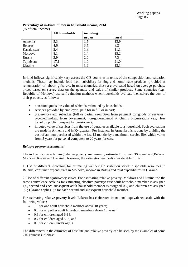
Working paper 4
Page 85
Percentage of in-kind inflows in household income, 2014
(% of total income)
All households including
urban rural
Armenia 5,3 1,5 13,9
Belarus 4,6 3,5 8,2
Kazakhstan 5,4 1,8 11,1
Moldova 8,1 1,4 15,2
Russia 2,9 2,0 7,3
Tajikistan 17,1 1,0 21,0
Ukraine 6,9 3,9 13,1
In-kind inflows significantly vary across the CIS countries in terms of the composition and valuation
methods. These may include food from subsidiary farming and home-made products, provided as
remuneration of labour, gifts, etc. In most countries, these are evaluated based on average purchase
prices based on survey data on the quantity and value of similar products. Some countries (e.g.,
Republic of Moldova) use self-valuation methods when households evaluate themselves the cost of
their products, as follows:
non-food goods the value of which is estimated by households;
services provided by employer , paid for in full or in part;
preferences and subsidies (full or partial exemption from payment for goods or services),
received in-kind from government, non-governmental or charity organizations (e.g., free
travel on public transport for pensioners);
imputed value of services from the use of durables available to a household. Such evaluations
are made in Armenia and in Kyrgyzstan. For instance, in Armenia this is done by dividing the
cost of an item purchased within the last 12 months by a maximum service life, which varies
from 5 years for personal computers to 20 years for cars.
Relative poverty assessments
The indicators characterizing relative poverty are currently estimated in some CIS countries (Belarus,
Moldova, Russia and Ukraine), however, the estimation methods considerably differ:
1. Use of different indicators for estimating wellbeing distribution series: disposable resources in
Belarus, consumer expenditures in Moldova, income in Russia and total expenditures in Ukraine.
2. Use of different equivalency scales. For estimating relative poverty, Moldova and Ukraine use the
same equivalence scale as for estimating absolute poverty: first adult household member is assigned
1,0, second and each subsequent adult household member is assigned 0,7, and children are assigned
0,5; Ukraine applies 0,7 for each second and subsequent household member.
For estimating relative poverty levels Belarus has elaborated its national equivalence scale with the
following values:
1,0 for one adult household member above 18 years;
0,8 for any other adult household members above 18 years;
0,9 for children aged 6-18;
0,7 for children aged 3- 6; and
0,5 for children under age 3.
The differences in the estimates of absolute and relative poverty can be seen by the examples of some
CIS countries in 2014:
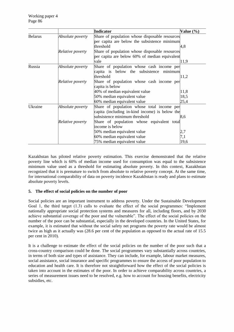
Working paper 4
Page 86
Indicator Value (%)
Belarus
Absolute poverty
Share of population whose disposable resources
per capita are below the subsistence minimum
threshold 4,8
Relative poverty
Share of population whose disposable resources
per capita are below 60% of median equivalent
vale 11,9
Russia Absolute poverty
Share of population whose cash income per
capita is below the subsistence minimum
threshold 11,2
Relative poverty
Share of population whose cash income per
capita is below
40% of median equivalent value 11,8
50% median equivalent value 18,5
60% median equivalent value 25,4
Ukraine Absolute poverty
Share of population whose total income per
capita (including in-kind income) is below the
subsistence minimum threshold 8,6
Relative poverty
Share of population whose equivalent total
income is below
50% median equivalent value 2,7
60% median equivalent value 7,1
75% median equivalent value 19,6
Kazakhstan has piloted relative poverty estimation. This exercise demonstrated that the relative
poverty line which is 60% of median income used for consumption was equal to the subsistence
minimum value used as a threshold for estimating absolute poverty. In this context, Kazakhstan
recognized that it is premature to switch from absolute to relative poverty concept. At the same time,
for international comparability of data on poverty incidence Kazakhstan is ready and plans to estimate
absolute poverty levels.
5. The effect of social policies on the number of poor
Social policies are an important instrument to address poverty. Under the Sustainable Development
Goal 1, the third target (1.3) calls to evaluate the effect of the social programmes: “Implement
nationally appropriate social protection systems and measures for all, including floors, and by 2030
achieve substantial coverage of the poor and the vulnerable”. The effect of the social policies on the
number of the poor can be substantial, especially in the developed countries. In the United States, for
example, it is estimated that without the social safety net programs the poverty rate would be almost
twice as high as it actually was (28.6 per cent of the population as opposed to the actual rate of 15.5
per cent in 2010).
It is a challenge to estimate the effect of the social policies on the number of the poor such that a
cross-country comparison could be done. The social programmes vary substantially across countries,
in terms of both size and types of assistance. They can include, for example, labour market measures,
social assistance, social insurance and specific programmes to ensure the access of poor population to
education and health care. It is therefore not straightforward how the effect of the social policies is
taken into account in the estimates of the poor. In order to achieve comparability across countries, a
series of measurement issues need to be resolved, e.g. how to account for housing benefits, electricity
subsidies, etc.
Working paper 4
Page 87
6. Metadata considerations
At national level, poverty lines are set using various definitions and methods. Terms such as “relative
poverty”, “absolute poverty”, “severe poverty” or “extreme poverty” should be used in conjunction
with their specific definitions. Metadata are needed to explain how national poverty lines were
determined, ensuring users can interpret the information correctly.
In measuring poverty, even variation in the base year can make the results hardly comparable. At the
international level, the standard measure of $1.25 (PPP) per day is used, measured in 2005 prices. In
the past, $1.00 per day and $1.08 per day, in 1993 prices, have been used. These changes show the
importance of including the metadata alongside the data, even if standard definitions are used. In an
MDG report, further details, such as the basket used for the PPP conversion, can be covered by a
reference.
Maintenance of good metadata is an important way of supporting cross-country comparability. Work
on monitoring MDGs has revealed that metadata are often missing, incomplete or incorrect. In some
cases, the exact or even broad definitions are missing. In several cases, the methodology is not clearly
specified and sometimes even the definition is not provided. Publishing the national poverty line
without any further specification makes comparative analysis difficult.
In general, data sources are listed in national reports. However, in several cases it is not clear to which
indicator or which period they refer. Important for the interpretation is a reference to the primary
sources. These are often missing or not specific enough. It is of imminent importance that such
metadata is available along with the poverty estimates provided in national reports.
7. (Tentative) Recommendations
1. Reach an international agreement on the poverty criteria, e.g. when using poverty thresholds
for the cost of basic food or non-food needs or when using certain percentage of the median
income.
2. Publish all the necessary metadata.
3. Disaggregate data whenever possible, especially with regard to the distinction between urban
and rural areas, age and sex. Differences in results may be extremely large, independent of the
threshold adopted.
________________
Related Documents