CHAPTER 2 MODELLING AND ANALYSIS OF DIGITAL BEAMFORMING ...shodhganga.inflibnet.ac.in/bitstream/10603/24772/7/07_chapter 2.pdf · 17 CHAPTER 2 MODELLING AND ANALYSIS OF DIGITAL BEAMFORMING

17

CHAPTER 2

MODELLING AND ANALYSIS OF

DIGITAL BEAMFORMING ALGORITHM

2.1. SMART ANTENNA BASICS

Smart antenna refers to a system of antenna arrays with smart signal

processing algorithm which is used to calculate beam forming vectors, to

track and direct the beam towards the mobile user (Jeffrey Reed 2002).

A smart antenna is a digital wireless communication antenna system that

takes the advantage of diversity effect at the source (transmitter), the

destination (receiver), or both. In conventional wireless communications, a

single antenna is used at the source, and another single antenna is used at the

destination. Such systems are vulnerable to problems caused by multipath

effects (Simon Haykins, 2002) such as fading and inter symbol interference

(ISI). In a digital communication system, multi-path fading and delay spread

lead to inter symbol interference (ISI) and co-channel interference (CCI). The

use of smart antennas can reduce or eliminate these problems resulting in

wider coverage and greater capacity. Most specifically, the features and

benefits of the smart antenna system include signal gain, interference

rejection, increase of coverage and capacity.

Smart antenna systems are customarily categorized as switched beam,

phased array, and adaptive array systems. Switched beam antennas are cheap,

but inflexible and use multiple small, immobile sub sectors. Base Station

selects one sub sector to use, based on strongest signal it receives. It suffers

18

from limited gain. Dynamically Phased Array/beam steering uses multiple

small, immobile sub sectors. It suffers from multipath interference. Whereas,

adaptive antenna array tracks the Direction of Arrival (DOA) and steers the

beam automatically towards the mobile user. Adaptive antennas origin in

radar applications some 40 years ago, and modern radar systems are

motivated the research in the area of mobile communication during the last

decades. While the requirements and the applicability are different in radar

and mobile communication applications, the solutions to key problems were

quite similar in both fields of research.

Adaptive antenna array system in its simplest form, consists of a

Uniform Linear Array (ULA) which are excited by a set of amplitude and

phase distributions determined by adaptive beamforming algorithm. The

block diagram is shown in 2.1. The adaptive beamforming algorithm along

with DOA algorithm optimizes the array output beam pattern, in such way

that maximum radiated power is produced in the direction of desired mobile

users, and deep nulls are generated in the direction of undesired signals

representing co-channel interference from mobile users in adjacent cells.

Figure 2.1 Block diagram of adaptive array system and its radiation

pattern

19

Adaptive antenna array technology uses a variety of signalprocessing algorithms to effectively locate and track several signals and todynamically minimize interference and maximize intended signal. Variousarray geometries are linear, circular and planar arrays. While a fixed-beamnetwork can choose a beam from a few predefined patterns, a fully adaptivearray has the flexibility in synthesizing the radiation pattern in any givendirection.

2.1.1 Wireless Multiple Access Techniques

One of the most important challenges with respect to wireless accessis the limited capacity of the air interface which is due to the fact that theavailable transmission bandwidth is finite. Therefore, in the field ofcommunications, the term multiple access could be defined as a means ofallowing multiple users to simultaneously share the bandwidth with leastpossible degradation in the performance of the system. The conventionalschemes are: FDMA, TDMA and CDMA. FDMA scheme provides onechannel per carrier, whereas TDMA allocates different time slots to differentsubcarriers using the same carrier frequency and thus interleaves signals fromvarious users in an organized manner. On the other hand, CDMA scheme is aspread spectrum method, that uses a separate code for each user. VariousCDMA signals occupy the same bandwidth and appear as random noise toeach other. In theory, the capacity provided by the three multiple access is thesame and is not altered by dividing the spectrum into frequencies, time slotsor codes (Godara, 1997). In practice, the performance of each system differs,leading to different system capacities. The SDMA scheme, also referred to asspace diversity, uses an array of antennas, in which simultaneous calls indifferent cells can be established at the same carrier frequency. The advent ofadaptive antenna array processing has the potential to combine SDMA alongwith TDMA, FDMA and CDMA to meet the requirements of third generationcommunication systems.

20

Orthogonal frequency multiplexing (OFDM) has emerged as a

successful air-interface technique for cellular based systems. OFDM is a

multicarrier modulation technique, a serial data bit stream is converted into

several blocks of data to be transmitted in different, parallel and orthogonal

subcarriers, subdividing the available bandwidth into narrowband

subchannels. Broadband wireless systems such as IEEE 802.11 (Wi-Fi) and

802.16d (Fixed WiMAX) have adopted OFDM because of its notable

advances on interference mitigating capabilities, robustness over frequency-

selective channels and simplicity of implementation. OFDMA maintain the

same benefits of OFDM and guarantees major scalability and MIMO

compatibilities in the fourth generation cellular systems (4G). Adaptive

antenna systems (AAS) may encompass different MIMO techniques such as

Space-Time Block Coding (STBC), beamforming and spatial multiplexing

(SM). For the open loop AAS, the multiple antennas can be used for STBC,

SM or combinations. When the closed loop AAS is employed, channel

reciprocity can be obtained in TDD mode, or feedback in FDD mode, the

multiple antennas can be used either for beamforming or for CL MIMO by

exploiting transmit antenna precoding techniques.

2.1.2 Uplink and downlink

Uplink beamforming is used to receive as much power as possible

from the desired user and as little power as possible from any undesired users.

Also, the downlink beamforming is used to transmit as much power as

possible to the desired user and as low power as possible to any undesired

users. For the application of adaptive antennas, FDD and TDD are well

known methods for transmission/reception. In FDD, transmission and

reception is performed at different frequencies, the radio channel is not

reciprocal. Additionally, small scale fading and channel statistics are not the

same in uplink and downlink. In the uplink case, the signal has already

21

propagated through the channel, and beamforming is performed at the place

of reception. In the downlink case, beamforming has to be performed before

the signal propagates through the channel. The channel information needed

for uplink beamforming is available at the smart antenna base station through

the pilot signal transmitted from each of the mobile terminals. However, since

the channel information of the downlink is not known to the base station, the

optimal parameters for the downlink beamforming are often borrowed from

the results obtained during the uplink.

A promising approach for the downlink, is to adaptively multiplex

user data onto an OFDM transmission system, where orthogonal time-

frequency resources are given to the user who can utilize them best, the

spectral efficiency will instead increase with the number of active users. To

implement downlink beamforminig, advanced systems like MIMO-

OFDM/SDMA and LTE need the knowledge of the channel state information

(CSI). This is obtained by TDD systems. In TDD system, uplink and

downlink transmission are time duplexed over the same frequency bandwidth.

Using the reciprocity principle it is possible to use the estimated uplink

channel for downlink transmission. Novel technologies such as orthogonal

frequency division multiplexing (OFDM) and Multiple Input Multiple Output

(MIMO), can enhance the performance of the current and future wireless

communication systems.

2.1.3 Adaptive beamforming in 4G Mobile Networks

3G and 4G cellular networks are designed to provide mobile

broadband access offering high quality of service as well as high spectral

efficiency. The main two candidates for 4G systems are WiMAX and

LTE(Carmen 2011). While in details WiMAX and LTE are different, there

are many concepts, features, and capabilities commonly used in both systems

22

to meet the requirements and expectations for 4G cellular networks. The

physical layer of both technologies use Orthogonal Frequency Division

Multiple Access (OFDMA) as the multiple access scheme together with space

time processing (STP) and link adaptation techniques (LA). In particular,

Space Time Processing has become one of the most studied technologies

because it provides solutions to ever increasing interference or limited

bandwidth (Paulraj & Papadias, 1997).

STP implies the signal processing performed on a system consisting

of several antenna elements in order to exploit both the spatial (space) and

temporal (time) dimensions of the radio channel. STP techniques can be

applied at the transmitter, the receiver or both. When STP is applied at only

one end of the link, Smart Antenna (SA) techniques are used. If STP is

applied at both the transmitter and the receiver, multiple-input, multiple-

output (MIMO) techniques are used. Both technologies have emerged as a

wide area of research and development in wireless communications,

promising to solve the traffic capacity bottlenecks in 4G broadband wireless

access networks (Paulraj & Papadias, 1997).

SDMA cellular systems have gained special attention to provide the

services demanded by mobile network users in 3G and 4G cellular networks,

because it is considered as the most sophisticated application of smart antenna

technology (Balanis, 2005) allowing the simultaneous use of any conventional

channel (frequency, time slot or code) by many users within a cell by

exploiting their position. OFDM combined with SDMA has been chosen as

multiple access for downlink in Long Term Evolution(LTE),(Hanzo et

al,2010). In order to cope with frequency selective channels, multiple transmit

and receive antennas can be readily combined with OFDM in the time domain

as space-time block coded(STBC-OFDM) and space frequency block

code(SFBC-OFDM) in frequency domain. OFDM-adaptive array system

23

beamforming can be applied to either time-domain or frequency domain.

Time domain beamforming is called pre-FFT because the array processing is

done before the FFT step and in the frequency domain process, beamforming

is done after FFT step(Heakle and Mangoud,2007). Borio(2006) suggests that

pre-FFT applied over the whole signal, requiring only one set of weights and

one FFT operator. In spite of its relative simplicity, the pre-FFT scheme offers

good results in most of the wireless applications.

The quality of a wireless link can be described by three basic

parameters, namely the transmission rate, the transmission range and the

transmission reliability. With the advent of MIMO assisted OFDM systems,

the above mentioned three parameters may be simultaneously improved. Next

generation cellular systems will have to provide a large number of users with

very high data transmission rates, and MIMO is a very useful tool towards

increasing the spectral efficiency of the wireless transmission. Akyildiz et.

al(2010) suggested that MIMO technology in LTE-Advanced are

beamforming, spatial multiplexing and spatial diversity. These techniques

require some level of channel state information(CSI) at the base station so that

the system can adapt to the radio channel conditions and significant

performance improvement can be obtained. MIMO systems may be classified

based on what type of CSI can be made practically available to the

transmitter. In general, transmit antenna algorithms can be classified as:

space time codes(need no CSI), MRC/blind adaptive beam steering (need full

CSI), adaptive beamforming algorithms(partial CSI). TDD systems gather this

information from uplink, provided that the same carrier frequency is used for

transmission and reception. The idea is to perform an intelligent SDMA so

that the radiation pattern of the base station is adapted to each user to obtain

the highest possible gain in the direction of that user. The intelligence

obviously lies on the base stations that gather the CSI of each user

equipment(UE) and decide on the resource allocation accordingly.

24

In communication systems that use OFDM and MIMO is

conventionally carried out on a subcarrier basis. There are two types of BF:

sub carrier wise and symbol-wise. The computational requirements are high

for each antenna. Hence symbol wise BF which performs the transmit and

receive BF operations in the time domain for the mitigation of co-channel

interference on spatially correlated channel(Pollok 2009). A novel iterative

algorithm may be incorporated at the base and mobile stations for the

computation of optimum weights which further increases system's capacity

and bandwidth efficiency, as well as in quality-of-service in mobile networks.

2.2 PROPAGATION CHARACTERISTICS AND CONSTRAINTS

2.2.1 Signal model

The message signal is usually modeled as discrete stochastic process

which is used to analyze a sequence of data that consists of the present

observation and past observation of the process. Most of the signals in the real

world are random, or contain random components due to factors such as

additive noise or quantization errors. For example, the sequence

)](),.......1(),([ Mnununu represents a partial discrete-time observation

consisting of samples of the present value and M past values of the process.

Its autocorrelation function is,

*( , ) [ ( ) ( )], 0, 1, 2,.r n n k E u n u n k k (2.1)

where E[.] denotes the expectation operator and * denotes complex conjugate.

This second-order characterization of the process offers two important

advantages. First, it lends itself to practical measurements and second, it is

well suited for linear operations on stochastic processes. The procedure for

estimating the parameters of a complex sinusoid with the help of correlation

matrix leads to the measurement of mean square value and auto correlation

25

matrix. The correlation matrix of a discrete-time stochastic process can be

defined as the expectation of the outer product of the observation vector u(n)

with itself. The dimension of the correlation matrix is M-by-M and is denoted

as R and it is written as:

nTunuER (2.2)

By substituting ‘u(n)’ into equation (2.2) and by using the property

defined in equation (2.1), the expanded matrix form of the correlation matrix

can be expressed as,

)0()2()1("""

)2()0()1()1()1()0(

rMrMr

MrrrMrrr

R (2.3)

2.2.2 Linear and constant envelope modulation schemes

The performance and the selection of the modulation scheme of a

cellular system is mainly depends on the power efficiency, spectral efficiency,

adjacent channel interference, BER performance and the implementation

complexity (Ali, 1999). Linear and constant envelope modulation techniques

such as QPSK and GMSK are popular in the cellular environment. QPSK is

predominantly noted for its spectral efficiency and it is used extensively in

CDMA cellular service and DVB (Digital video broadcasting). GMSK is a

constant envelope modulation scheme which avoids the linearity

requirements, but the spectral efficiency is lower, and it is used in GSM,

DECT and DCS. The RF band width is controlled by the Gaussian low-pass

filter bandwidth and the bandwidth efficiency is less than QPSK. However,

QPSK effectively utilizes bandwidth; whereas, GMSK requires more

26

NRZ signal

X

X

AcCos(wct)

AcSin(wct)

QPSK signal90°

bandwidth to effectively recover the carrier. Both QPSK and GMSK have

strong features that provide a desirable cellular environment.

Most digital transmitters operate their power amplifiers at or near

saturation to achieve maximum power efficiency. At saturation, it poses a

threat to the signal, exposing it to phase and angle distortions. These

distortions spread the transmitted signal into the adjacent channel, causing

interference. To resolve this issue, a filter is used to suppress the side lobes.

Nyquist pulse-shaping techniques, such as the Raised Cosine (RC) filter and

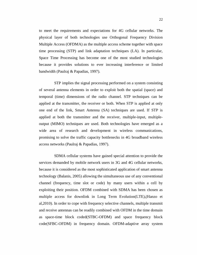
Gaussian filter, are used to reduce ISI. Figure 2.2 is the block diagram of

generation of QPSK signal.

Figure 2.2 QPSK modulator

First, the system converts a bit stream into a Non-Return-to-Zero

(NRZ) signal which is multiplied by an in-phase (I) and quadrature (Q) signal,

keeping in mind that each carrier phase is separated by 90°. The two

components are then summed to achieve the desired QPSK signal output. In

order to optimize the signal, QPSK uses the RC filter. This prevents the signal

from spreading its energy into the adjacent channels. Ideally, the Nyquist

filter is free of ISI. However, all practical Low Pass Filters (LPF) exhibit

27

NRZsignal

Integrator

Gaussianfilter

Differentialencoder

Cos() X

Cos(wct)

InputOutput

d(k)

Sin() X

Sin(wct)

phase and amplitude distortions so special pulse shaping filters are needed to

ensure that the total transmitted signal arrives at the receiver. As the roll-off

factor of the RC filter decreases, the spectrum becomes more compact. This

requires a more complex receiver at demodulation. However, since QPSK is

predominantly noted for its bandwidth efficient feature, it is preferable to

operate at higher values of roll-off in order to accommodate for the increasing

demand for more users within a limited channel bandwidth. Nevertheless,

another tradeoff is that a complex receiver is needed at the end of the filter to

recover the carrier.

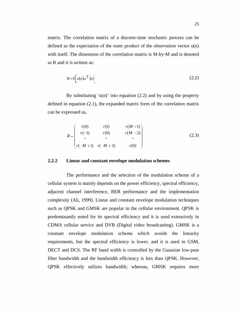
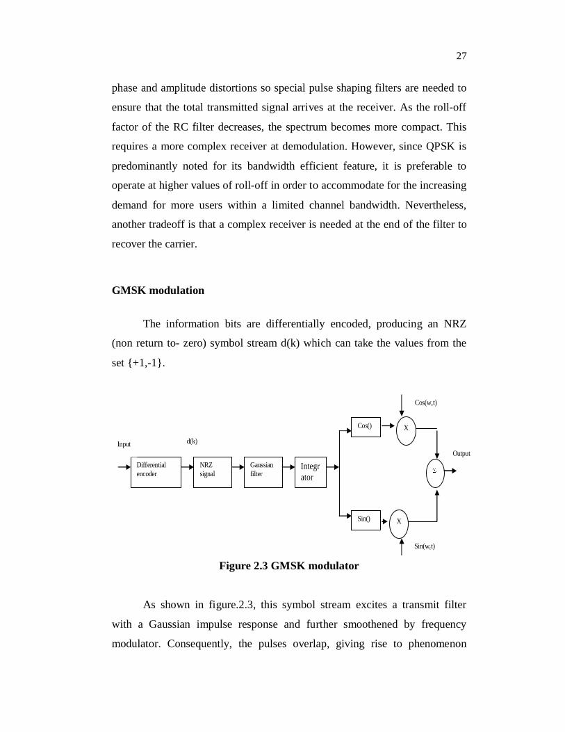
GMSK modulation

The information bits are differentially encoded, producing an NRZ

(non return to- zero) symbol stream d(k) which can take the values from the

set {+1,-1}.

Figure 2.3 GMSK modulator

As shown in figure.2.3, this symbol stream excites a transmit filter

with a Gaussian impulse response and further smoothened by frequency

modulator. Consequently, the pulses overlap, giving rise to phenomenon

28

known as ISI. The extent of overlap is determined by the product of

bandwidth of Gaussian filter and data bit duration; the smaller the bandwidth

bit time product (BT), the more the data bits or pulses overlap (Diana, 2000).

A gaussian pulse is good choice of shaping function since it provides a

particularly compact frequency domain spectrum which in turn eliminates the

broad pattern of side lobes of a rectangular pulse (Berger, 2006). Filtering

allows the transmitted bandwidth to be significantly reduced without losing

the content of the digital data. This improves the spectral efficiency of the

signal.

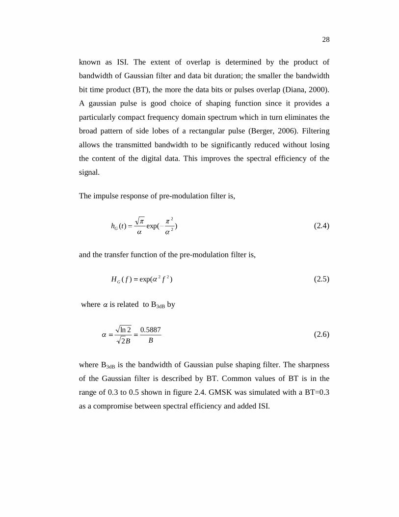
The impulse response of pre-modulation filter is,

)exp()( 2

2

thG (2.4)

and the transfer function of the pre-modulation filter is,

)exp()( 22 ffHG (2.5)

where is related to B3dB by

BB5887.0

22ln (2.6)

where B3dB is the bandwidth of Gaussian pulse shaping filter. The sharpness

of the Gaussian filter is described by BT. Common values of BT is in the

range of 0.3 to 0.5 shown in figure 2.4. GMSK was simulated with a BT=0.3

as a compromise between spectral efficiency and added ISI.

29

-40 -30 -20 -10 0 10 20 30 400

0.2

0.4

0.6

0.8

1

1.2

1.4

Time

Impulse response of Gaussian filter

BT=0.3

BT=0.5

Figure 2.4 Gaussian Pulse shape

The impulse response of the filter to rectangular signal of duration ‘T’ is

)2ln22()

2ln22(

21)(

TtBQ

TtBQ

Ttg (2.7)

where Q(t) is a function,

dxxtQ )2

exp(2

1)(2

, (2.8)

and B is the bandwidth of low pass filter having a Gaussian shaped spectrum.

As with any natural resource, it is important to make use of RF spectrum by

using channel bands that are too wide. Therefore narrower filters are used to

reduce the occupied bandwidth of the transmission.

Due to its linear amplification feature, QPSK is able to maintain

low spectral sidelobes; thus providing good adjacent channel performance.

This is an important contribution to wireless systems because it

30

enables a higher channel reuse factor. Furthermore, QPSK’s importance in

CDMA is evident with its efficient bandwidth use, enabling more users

within a limited channel bandwidth. GMSK makes its contribution to

cellular systems in communications from the mobile to the base station. In

the case of uplink, power is drained significantly from the mobile,

necessitating a power efficient amplifier. GMSK fulfills this need.

Furthermore, due to its frequency modulating characteristics, GMSK shows

a greater immunity to signal fluctuations. If most efficient bandwidth

utilization and moderate hardware complexity is the key requirement, QPSK

will be better choice. Out of band power, tolerance against filter parameters

and non linear power amplifiers are important features, GMSK is the best

solution (Mundra 1993). QPSK and GMSK each provide beneficial features,

and although neither dominates the other, both contribute to the

advancement of wireless telecommunication systems. Hence, the proposed

system is analyzed with both of the modulation schemes.

2.2.3. Wireless channel

Free space propagation occurs when a unique direct signal path

exists between a transmitter and a receiver. Reflection, refraction, diffraction

and scattering determine the presence of many signal replicas at the receiver,

leading to the phenomenon referred to as multipath. Besides, the complexity

of the scenario is increased by the effects due to mobility, which cause short

term fading and long term fading of the received signal. In a multipath

scenario, each signal component is characterized by its amplitude, phase shift,

delay and direction of arrival (DoA). When there is no direct path between

transmitter and receiver, the entire received field is due to multipath. The

inphase component, )(txI and the quadrature component, )(txQ , of the

incoming signal is modeled as complex Gaussian random process. These two

processes have zero mean because of the absence of LOS between transmitter

31

0 200 400 600 800 1000 1200 1400 1600 1800 2000-20

-15

-10

-5

0

5

10

sample index

and receiver. The channel is modeled in complex base band signal asN

i

tfcji

iieAN

tc1

)2(1)( where ‘Ai’ is the amplitude

of the ith complex sinusoid and i is the random phase uniformly distributed

from zero to 2 , ‘f’ is the Doppler frequency shift. Thus the statistics of the

envelope )()(( 22 txtx QI follows a Rayleigh distribution,

otherwise

zeP

z

z

rxPz

rx

FAD .............0

..0........

2

)(

2

(2.9)

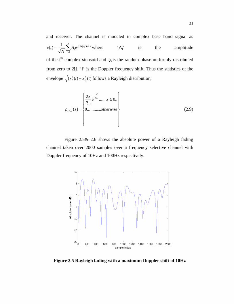
Figure 2.5& 2.6 shows the absolute power of a Rayleigh fading

channel taken over 2000 samples over a frequency selective channel with

Doppler frequency of 10Hz and 100Hz respectively.

Figure 2.5 Rayleigh fading with a maximum Doppler shift of 10Hz

32

Experimental studies have shown that Rayleigh fading is a proper

model for heavily built-up urban environment, characterized by the presence

of rich scattering and absence of LOS between the communication nodes.

2.2.4 Vector Channel modeling

For design, simulation, and planning of wireless systems, the

physical process by which the signals are received at the array may be

modeled as narrowband or broadband.

Narrow band Array

It is important to recognize the narrowband model to describe the

difference in the signal received at one antenna relative to another antenna.

Consider a situation where a plane wave is received at multiple antennas as

shown in figure 2.7. In this two-dimensional representation, the signal

observed at one antenna will be delayed version of the signal observed at

some other antenna. Let antenna ‘1’ be the reference antenna. The signal

0 200 400 600 800 1000 1200 1400 1600 1800 2000-50

-40

-30

-20

-10

0

10

sample index

Figure 2.6 Rayleigh fading with a maximum Doppler shift of 100Hz

33

Incidentwave

First and kth antennaelements

Incidentwave fronts

x

y

1 k

kd

sinkd

observed at this antenna is given by,

x 1(t) = G1( ) r (t)+ n 1(t) (2.10)

where r (t) is the incident signal and n 1(t) is the measured noise for the first

antenna. The quantity denotes the plane wave’s direction of arrival (DOA)

and G1( ) is the gain for the first element at DOA . The signal observed at

the kth antenna is k k k kx (t) G ( ) r (t ) n (t) (2.11)

Figure 2.7 Narrow band model of received signals

where k is the time difference of direction of arrival(TDOA). From

figure 2.7,

kk

d sinc

(2.12)

where dk is the separation of the first and kth antennas and ‘c’ is the velocity

of the incident wave. Therefore, for sufficiently small values of k ,

kr(t ) r(t) (2.13)

34

The above equation is called the narrowband array approximation. The phase

shift is in terms of the signal carrier wavelength c ,

k kk c k

c c

2 c d sin 2 d sinc

(2.14)

Assuming that the received signal is in a complex base band representation,

we have

k kr(t ) a ( )r(t) , where, kjkk e)(G)(a (2.15)

The signal experienced at each element can be represented in vector form as

1 1 1

M M M

x (t) a ( )r(t) n (t). .

x(t) . . a( )r(t) n(t). .x (t) a ( )r(t) n (t)

(2.16)

where Tjjk

KiK eea ],......,1[)( )()(1 is the array steering vector towards the

direction k. )( kiis the propagation delay between the first and the ith

element for a waveform coming from direction k. TM tntntn )](),......([)( 1

is

the noise vector.

Broadband model

The broadband beamformer structure is shown in figure 2.8. It

samples the propagating wave field in both space and time and is often used

when signals of significant frequency extent (broadband) are of interest (Van

Veen and Buckley, 1988). The outputs are expressed as,

35

J

i

K

pipi pTtxwty

1

1

0

*, )()( (2.17)

where K-1 is the number of delays in each of the J sensors channels and T is

the duration of a single delay. In vector form: )()( txwty H where

Tj TKtxtxTKtxTtxtxtx ])1((),....(),...)1((),......(),([)( 2111

TKJK wwwwww ],...,...,....,[ )1(,0,2)1(,11,10,1 . The frequency response of the system

with tap weights Jpwp 0,* and a tap delay of T seconds is given by,

)1(*)( pTjpewwr or )()( dwr H (2.18)

Assume that the signal is a complex plane wave with DOA ‘ ’ and

frequency ‘ ’. For convenience let the phase be zero at the first sensor. This

implies that .2,)()( )]([1 Jlekxandekx lkj

lkj

)(l represents the time delay due to propagation from the first to thethl sensor. Substitution into eqn 2.17 results in the beamformer output

),()( ])([*, reeweky kjpjpl

kj l (2.19)

where ),(r is the frequency response represented in the vector form as

),(),( dwr H .

36

2.2.5 Channel State Information (CSI)

In wireless communication, channel state information (CSI) refers to

known channel properties of a communication link. CSI needs to be estimated

at the receiver and usually quantized and fed back to the transmitter.

Therefore, the transmitter and receiver can have different CSI. Since the

channel conditions vary, instantaneous CSI needs to be estimated on a short

term basis. A popular approach is called training sequence, where a known

signal is transmitted and the channel matrix H is estimated using the

combined knowledge of the transmitted and received signal. In multi antenna

communication, the receiver can accurately track the instantaneous state of

the channel from pilot signals that are typically embedded within the

Figure 2.8 Broad-band beamformer structure

Weightcontrol

Errorsignal

y(t)

TT

w1 w12

TT

w2 w2

TT

Wj1 Wj2

W 1,K-1

W 2,K-1

W j,K-1

X1(t)

X2(t)

XJ(t)

37

transmissions. In practice, the CSI available at the transmitter is subject to

errors caused by limited channel state feedback, estimation errors, short

channel coherence time etc. The system model of channel estimation is shown

in figure 2.9.

Channel estimation is done at the receiver during the training phase.

The estimated channel values are also fedback to the transmitter. The

transmitter adapts the beamforming vector based on the predicted channel

values. The delay involved in the feedback and the time varying nature of the

wireless channel together lead to a different channel at the time of

transmission than the channel that is fedback. Therefore, the adaptation at the

transmitter is done based on the past channel values.

The idea behind channel prediction is to use past and present

channel samples to predict future power level of the Rayleigh channel. In a

narrowband flat-fading channel, the system is modeled as

nHxy (2.20)

where ‘y’ and ‘x’ are the receive and transmit vectors, respectively, and ‘H’

and ‘n’ are the channel matrix and the noise vector, respectively. Since the

channel conditions vary, instantaneous CSI needs to be estimated on a short-

term basis. A popular approach is so-called training sequence (or pilot

Figure 2.9 Channel state information-system model

ChannelEstimation

Symbol Detection

Feedback channel

AdaptiveBeamforming

38

sequence), where a known signal is transmitted and the channel matrix H is

estimated using the combined knowledge of the transmitted and received

signal. Wajid (2009) suggested downlink beamforming using perfect

instantaneous and covariance based CSI are the suitable methods to estimate

CSI. In practice, the CSI available at the transmitter is subject to errors caused

by limited channel feedback, estimation errors and short channel coherence

time etc. Generally, there are two types of channel estimators: Least squares

estimators (LSE) and Minimum mean square estimator (MMSE).

LS is a simple method for estimation and it is used as an initial step.

Yucek (2007) suggests least squares (LS) method for OFDM signal, whose

LS estimate of the channel frequency response (H) can be calculated using

the received signal and the knowledge of the transmitted symbols as,

)()()(

)()()(ˆ

kXkWkH

kXkYkH LS (2.21)

If the channel and noise distributions are unknown, then the least-

square estimator (also known as the minimum-variance unbiased estimator)

is,

1)( HHestiamteLS PPYPH (2.22)

where ()H denotes the conjugate transpose and the training matrix

],....[ 1 NPPP .

The received SINR of the ith user can be written as

K

illiii

Hi

iiHi

wRw

wRwSINR

,1

2 (2.23)

39

where }{ Hiii HHER is the downlink channel covariance matrix for the ith

user. If the channel co-variance matrix assumed to be perfectly known, the

downlink beamforming is subjected to the condition:

iK

illiii

Hi

iiHi

k

kk

wRw

wRww

,1

2

2

1

min (2.24)

where i is the minimum acceptable SINR for the ith user. . denotes the

Euclidean norm of a vector.

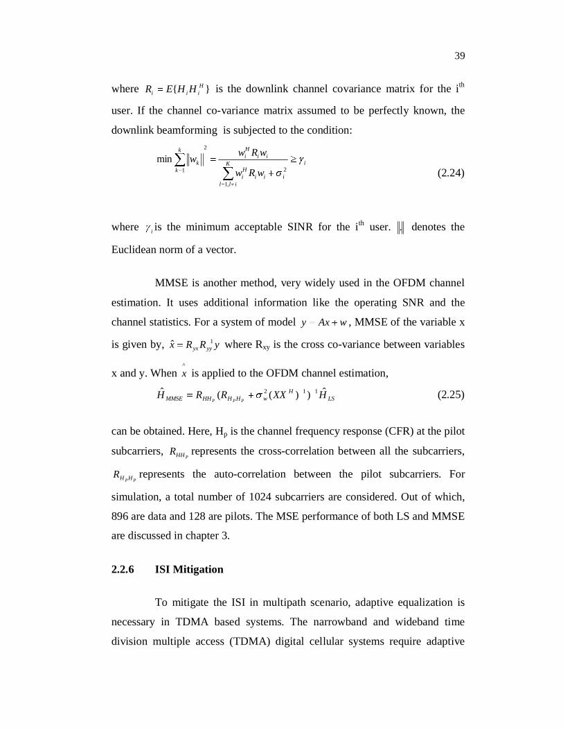
MMSE is another method, very widely used in the OFDM channel

estimation. It uses additional information like the operating SNR and the

channel statistics. For a system of model wAxy , MMSE of the variable x

is given by, yRRx yyyx1ˆ where Rxy is the cross co-variance between variables

x and y. When^x is applied to the OFDM channel estimation,

LSH

wHHHHMMSE HXXRRHPPP

ˆ))((ˆ 112 (2.25)

can be obtained. Here, Hp is the channel frequency response (CFR) at the pilot

subcarriers,PHHR represents the cross-correlation between all the subcarriers,

PPHHR represents the auto-correlation between the pilot subcarriers. For

simulation, a total number of 1024 subcarriers are considered. Out of which,

896 are data and 128 are pilots. The MSE performance of both LS and MMSE

are discussed in chapter 3.

2.2.6 ISI Mitigation

To mitigate the ISI in multipath scenario, adaptive equalization is

necessary in TDMA based systems. The narrowband and wideband time

division multiple access (TDMA) digital cellular systems require adaptive

40

equalization at the demodulator to combat the ISI resulting from the time-

variant multipath propagation of the signal through the channel. Whereas,

OFDM is the promising technique to combat multipath in receiver.

2.2.6.1 Equalization

An equalizer is a compensator for channel distortion. For

communication channel in which the channel characteristics are known or time

varying, optimum transmit or receive filters can not be designed directly. For

these cases, an equalizer is needed to compensate for the ISI created by the

distortion in the system. There are three types of equalization methods

commonly used: Maximum Liklihood (ML) detection, Linear equalization,

Non linear equalization. Linear equalizers are easy to implement and effective

where the ISI is not severe (using Zero forcing rule or mean square error

criterion). Adaptive equalization will be needed to overcome the severe ISI

affecting transmission at high data rate rates. In addition to the ISI due to

multipath, spectrally efficient GMSK introduces considerable amount of

controlled phase ISI. Hence, the LMS or Gradient equalizer is used to

implement adaptive equalization. It is a stochastic gradient optimization

algorithm based on traditional optimization technique called method of

Steepest Descent. The LMS algorithm is basically a simplification of the

Method of Steepest Descent, where instantaneous values are used instead of

actual values. The weight update equation,

][*][]1[ nYnwnw i (2.26)

where Ti TMnYYTMnYnY )])((.....,),........0(,........)(([][ represents the tap-

inputs at the time instant(or iteration). The error ][n is computed from the

equalized output using either a training sequence or the decoded output as

reference.

41

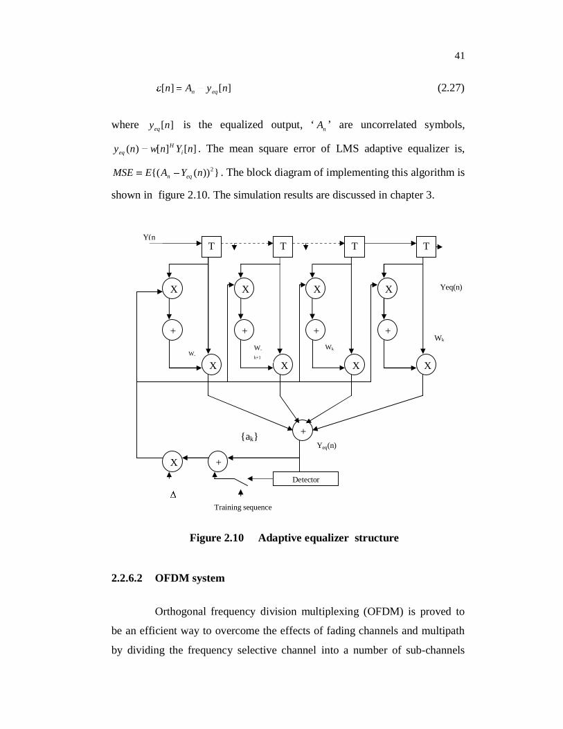
][][ nyAn eqn (2.27)

where ][nyeq is the equalized output, ‘ nA ’ are uncorrelated symbols,

][][)( nYnwny iH

eq . The mean square error of LMS adaptive equalizer is,

}))({( 2nYAEMSE eqn . The block diagram of implementing this algorithm is

shown in figure 2.10. The simulation results are discussed in chapter 3.

2.2.6.2 OFDM system

Orthogonal frequency division multiplexing (OFDM) is proved to

be an efficient way to overcome the effects of fading channels and multipath

by dividing the frequency selective channel into a number of sub-channels

Yeq(n)

T

X

X

+

T

X

X

+

T

X

X

+

T

X

X

+

+

+XDetector

Y(n

WkWkW-

k+1W-

Yeq(n){ak}

Training sequence

Figure 2.10 Adaptive equalizer structure

42

corresponding to the OFDM sub-carrier frequencies. In order to increase the

spectral efficiency in OFDM systems and to promote the interference

suppression in multipath channels, a multiple antenna array can be used at the

receiver (Borio, 2006). In an OFDM system, the beamforming algorithm can

be applied in either time domain or frequency domain. Time domain array

processing has lower complexity, because only one FFT is required. Time

domain beamforming is called pre-FFT beamforming because the array

processing is done before the FFT step in time domain, and frequency domain

beamforming can be called post FFT because the array processing is done

after the FFT step in frequency domain. Post-FFT requires set of weights for

each array branch, so that the total number of weights processed is equal to

the number of elements times the number of sub carriers, which requires a

high computational complexity. Even though, Borio and Ribeiro (2006)

suggested that pre-FFT can be performed with conventional LMS, RLS and

SMI algorithm with appreciable BER, the development of suitable adaptive

algorithm may further improves the performance of the system.

At the transmitter (figure 2.11), the input random data is converted

from serial to parallel and then mapped to any one of the modulation types

(BPSK, QPSK, 16QAM, 64QAM). The obtained N samples are then passed

through the IFFT block. Cyclic prefix (CP) was added to the data once the

data was converted into time domain and ready to be transmitted. The

addition of the CP (of lengths such as ¼, 1/8, 1/16 and 1/32) to the data before

it was actually transmitted to cater the problems related to the multipath

propagation and provided a resistance against ISI. The transmitted data is then

fed to the channel.

43

Random datagenerator

Modulator(BPSK,QPSK,16QAM,64QAM)

Cyclic PrefixInsertion

IFFT

Figure.2.11 OFDM Transmitter functional scheme

In order to design an efficient wireless channel, multipath spread,

fading characteristics, path loss, doppler spread and co-channel interference

are the important factor to be kept in mind. As a result, the transmitted OFDM

signal suffers from multipath effects and other channel effects. At the

receiver, an array of antennas are deployed. The received signal is passed

through a beamformer which is located before the FFT stage. The process

starts with the removal of the cyclic prefix that was initially added to the

transmitted signal as earlier explained in the transmitter module. After cyclic

prefix removal, the data was converted back into frequency domain from the

time domain using the FFT. Once the data conversion is completed, the data

is passed to the de-modulator where the data is demodulated according to

modulation schemes applied on the data during the transmission. The de-

modulated data is analyzed and compared to the original data by Bit-Error-

Rate (BER) calculator.

Figure.2.12 Pre-FFT beamforming scheme

y k[j]

w k,1

w k,2

r k,1[n]

r k,2[n]

w k,L

Cyclic prefixsuppression

Pre-FFT Beamformer

y k[n]

r k,L[n]

+ FFTCyclic prefixsuppression

Cyclic prefixsuppression

44

A Pre-FFT beamformer (figure 2.12) was employed as spatial

processing at reception. Each replica of the received signal rk,h[n] is multiplied

by the conjugate of a complex weight wk,h[n] and then summed up to form the

spatially filtered signal y[n]. In this method, the array weighting is applied

over the whole signal in time domain, that is, before FFT operation. The base

band sampled signal at the output of the pre-FFT beamformer is obtained by a

linear combination of the components directly detected by the K elements.

The array weighting process in pre-FFT scheme can be expressed, in vectorial

notation, as : ][][ mrwmy H , where ‘w’ is the 1K is the complex weight

vector. In this scheme, the complex weights are determined by a suitable

adaptive algorithm which minimizes the mean square error (MSE). In order to

evaluate the MSE, a reference signal is needed, which is a pilot tone

embedded into the OFDM frame.

}{2

kHk

T XwsEMSE (2.28)

The beamforming weight set ‘wk’ that minimizes the above

equation and nullifies the MSE gradient and hence the performance of the

system is improved.

2.3 DIGITAL BEAMFORMING ALGORITHMS

The increasing demand for mobile communication services in a

limited RF spectrum motivates the need for better techniques to improve

spectrum utilization in terms of digital beamforming algorithm. This

challenging scenario involves the emerging 4G technologies like World wide

interoperability of Microwave Access (WiMAX), and Long term Evolution

(LTE). However, in order to satisfy the increasing demand of network

capacity, the exploitation of the spatial domain of the communication channel

by means of multiple antenna system is followed (Godara, 1997). This can be

45

a key improvement for enhancing the spectral efficiency of the wireless

systems. Spatial Division Multiples Access (SDMA) cellular systems have

gained special attention to provide the services demanded by mobile network

users in 3G and 4G cellular networks, because it is considered as the most

sophisticated application of smart antenna technology (Balanis, 2005)

allowing the simultaneous use of any conventional channel (frequency, time

slot or code) by many users within a cell by exploiting their position.

Basically, Digital beamforming is the marriage of antenna

technology and digital technology. Digital beamforming need a reference for

the underlying principle to compare their operation’s outcome with some

desired property of the received signals. This reference may be of temporal or

spatial nature. Generally the goal of the adaptive beamforming is to optimize

the beamformer response, so the output contains only minimal contribution

due to noise and signals arriving from other than the desired signal direction.

This is performed by choosing weights based on the statistics of the data

captured by the array according to some optimum criterion. Adaptive

beamforming method may be roughly divided in to different classes according

to their reference they use to adaptively determine the weights. Historically,

temporal reference based algorithms were used. This class of algorithms relies

on the existence of a reference or training sequence embedded within the data

stream. To exploit the information and to estimate the direction of arrival,

spatial reference is also needed.

2.3.1 Temporal Reference algorithms

This class of adaptive algorithms is designed to act as a spatial (or

spatio-temporal in the wideband case) filter, in such a way, that complex

weights are calculated directly from the statistics of the received array data.

To do so, an error signal is minimized by adjusting complex weights in a

continuous, iterative, or in a block-wise fashion. To adjust the weights in an

46

optimum way, it is necessary to know enough about the desired signal, called

temporal reference. A generic adaptive beamforming system is shown in

figure 2.13. Conventional adaptive beamforming algorithms such as least

mean square (LMS), constant modulus algorithm (CMA), recursive least

square (RLS) have been simulated and analyzed using ULA of eight

elements.

(i) Least Mean Square algorithm (LMS)

One of the simplest algorithm for adaptive processing is based on

least mean square (LMS) algorithm for continuous adaptation. The LMS

algorithm is stated by the following equations:

Output vector, ][][][ nxnwny H

Error vector, ][][][ nyndn

Weight update vector, ][][][]1[ * nnxnwnw (2.29)

where ][nx is the input data sequence, ][ny is the output sequence,‘ w ’ is the

update weight vector and ][nd is the desired signal sequence. It has been

shown that starting with an arbitrary initial weight vector, the LMS algorithm

will converge and stay stable as long as the value of is chosen

as:max

10 where max is the maximum eigenvalue (or trace) of the

Covariance Matrix. Within the margin, the larger the value of , faster the

convergence but less stability around the minimum value. On the other hand,

smaller the value of , slower the convergence but the algorithm will be

more stable around the optimum value. When the eigenvalues are

widespread, convergence can be slow.

47

(ii) Recursive Least Squares algorithms (RLS)

The recursive least squares (RLS) algorithm offers an alternative to

the LMS algorithm as a tool for solution of adaptive filtering problems. The

fundamental difference between the RLS algorithm and the LMS algorithm

may be stated as: The step size parameter in the LMS algorithm is replaced

by the inverse of the correlation matrix of the input vector x(n), which has the

effect of whitening the tap inputs. The convergence behavior of the RLS

algorithm is as follows:

i. The rate of convergence of the RLS algorithm is typically in

an order of magnitude faster than that of the LMS algorithm.

ii. The rate of convergence of the RLS algorithm is invariant to

the eigen value spread of the ensemble average correlation

matrix of the input vector x(n).

iii. The excess mean-square error of the RLS algorithm converges

to zero as the number of iterations ‘n’, approaches infinity.

(iii) Constant Modulus Algorithms (CMA)

When training sequences are unavailable, blind algorithms become

attractive. Generally, these techniques exploit some known property of the

desired signal so that an indirect measure of the output SINR can be obtained.

The constant modulus algorithm (CMA) is perhaps the most well-known

blind algorithm and is used in many practical applications, because it requires

no carrier synchronization (Tong 1998). In general, the CMA seeks a beam-

former weight vector that minimizes a cost function of the form

p qpq nJ (| y | 1) . (2.30)

48

The weight update equation is,

w(n 1) w(n) (n)x(n 1) (2.31)

A particular choice of p and q yields a specific cost function, called

the (p, q) CMA cost function. The objective of CM beamforming is to restore

the array output ‘yn’ to a constant envelope signal.

2.3.2 Performance comparison of conventional algorithms

Literature suggests numerous adaptive algorithms and diversity

algorithms for beamforming applications (Reed, 2006). The best algorithm for

the particular array must not only account for the signal environment at hand,

but also for a number of other practical considerations including

synchronization, the presence or absence of array data, the computational

complexity and hardware cost. Signal environment considerations include the

nature of the desired signal’s channel, its SNR, number of interfering signals

as well as their powers and DOAs relative to their desired signal. Hence, there

is no algorithm which satisfies all the above requirements.

In this chapter, some of the blind and non-blind adaptive algorithms

are analyzed based on their performance in the given channel conditions and

various parameters like HPBW, percentage of power in the side lobe, null

point suppression and number of iterations required to optimize the weight

vectors are compared. Let us analyze one by one. LMS is simple and less

complex. If the input vector and desired response are available at each

iteration, the LMS algorithm is generally the best choice for many

applications of adaptive signal processing (Reed, 2006).

The CMA cost function is most important since noise and

interference compute the constant modulus property of the desired signal

(Denno, 2004).

49

A potential drawback of the CMA is the capture effect. In an

environment containing multiple CM signals, a CMA beamformer will

typically extract the strongest signal. This may or may not be the desired

signal. To extract the original signal, the successive interference cancellation

is made so as to determine the original signal. The only difficulty of the RLS

algorithm is the update of the inverse data co-variance matrix. The RLS

computation is obtained for three different cases, i.e. high SNR (SNR = 30dB

or more), medium SNR (Input SNR 10dB) and low SNR.

All the cellular mobile applications use the 120o sector for the

coverage of users, hence the calculations are obtained for -60o to +60o. The

various parameters such as HPBW, side lobe level, null levels and the

convergence rate are calculated by assuming the desired user and the

interferers are moving in the scanning sector of -60o to 60o, and they are

tabulated (Tables 2.1). From the observations, LMS and RLS are found to be

better compared to other conventional algorithms.

Table 2.1 Advantages and performance of conventional algorithms

Algorithm Advantage HPBW (Deg) Side lobelevel (dB’s)

Null levels(dB’s)

LMS Simple stable, lowcomplexity 17-18 -12 to -15 -25 to -30

RLS Update of the inverse dataco-variance matrix 18-20 -14 to -15 -25 to -40

CMANo carrier synchronization,robust to symbol timingerror

23-25 -12 to -18 -25 to -35

Wiener Depends on the update ofco-variance inverse matrix 18-20 -13 to -14 -20 to -30

MVDR

Minimum powercontributed by noise andinterference, fixed gain,max SNR in desireddirections,

20-25 -13.5 to -15 -30 to -35

50

Drawbacks of conventional algorithm

Each of the conventional algorithms has its own advantage and

disadvantage. From the above Table 2.1, it is understood that the HPBW is

larger (Simon 2002), approximately from 17o to 25o and side lobe level is at

an average of 13.5dB. The classical RLS algorithm uses the constant

forgetting factor 0< <1, this achieves low misadjustment and good stability,

but its tracking ability is poor. The recursive equation for updating the tap-

weight vector of RLS algorithm is based on Kalman gain and posteriori error

which in turn depends on forgetting factor ‘ ’. A smaller value of forgetting

factor improves tracking, but also increases misadjustment, which could

affect the stability of the algorithm. The Weiner solutions require the

computation of inverse of the array correlation matrix (Rxx-1) and the

calculation of output vector. Normally, inverse matrix operation affects the

convergence rate and the speed of the algorithm.

The unconstrained LMS is not subjected to constraints at each

iteration, but it estimates the gradient of MSE quadratic error and then

moving the weights in the opposite direction with respect to the gradient by a

small quantity, which is determined by a constant step size. This step size

largely influences the convergence characteristic of the algorithm in terms of

speed and closeness to the optimal solution. The selection of a too small step

size results in a lower rate of convergence. The main draw back of the LMS is

its sensitivity to the convergence behavior.

Constant modulus (CMA) algorithm operates on the principle that

the amplitude of the communication signal is distorted by interference and

multipath fading. The main drawback of the CMA is, in hostile environment,

the algorithm may incorrectly select an interferer having the same envelope of

the desired signal. CMA is a gradient based algorithm which works on the

51

premise that the existence of interference causes fluctuation in the amplitude

of the array output.

2.3.3 Spatial Reference algorithm

This class of algorithm estimates the direction of arrival (DOA)

from the available samples. This can be done either by eigen value

decomposistion of the estimated array correlation (covariance) matrix, or by

singular value decomposition of the array data matrix.

Direction of Arrival (DOA) algorithm

In an adaptive array antennas, to locate the desired signal, some

popular direction of arrival estimation algorithms such as MUSIC and

ESPRIT are used. MUSIC and ESPRIT DOA estimation algorithms provide

high angular resolution and hence they are explored by various parameters of

the adaptive antenna system. Literature suggests that MUSIC algorithm is

highly accurate and stable and provides high angular resolution compared to

ESPRIT and hence MUSIC can be widely used in mobile communication to

estimate the DOA of the arriving signals.

Multiple Signal Classification (MUSIC) Algorithm

The MUSIC method is a relatively simple and efficient eigen

structure method of DOA estimation. This method estimates the noise

subspace from the available samples by either eigenvalue decomposition of

the estimated array correlation matrix or singular value decomposition of the

data matrix. Once the noise subspace has been estimated, a search for ‘M’

directions is made by looking for steering vectors that are orthogonal to the

noise subspace. In narrowband condition, if M signals impinge on an L

52

dimensional array from distinct DOAs M,......., 21 , the array model may be

written as ,

)()()()( tntsAtx (2.32)

where )](,....(),([)( 21 MaaaA is the steering matrix,T

M tstststs )](....),........(),([)( 21 denotes the baseband signal waveforms, and

n(t) is spatial white noise. The spatial covariance matrix:

)}()({ txtxER H

= )}()({)}()({ tntnEAtstsAE HHH

= IASAH 2 (2.33)

where )}()({ tstsES H is the source covariance matrix; )}()({ tntnE H I2 is

the noise covariance matrix , that is a reflection of the noise having a common

variance 2 at all sensors and being uncorrelated among all sensors. This is

normally accomplished by searching for peaks in the MUSIC spectrum given

by,

)()()()()(aUUa

aaP HNN

H

H

MUSIC (2.34)

or, alternatively,

)()(1)(

aUUaP H

NNHMUSIC , (2.35)

where UN denotes an L by L-M dimensional matrix with its L-M columns

being the eigen vectors corresponding to the L-M smallest eigenvalues of the

array correlation matrix, and a denotes the steering vector corresponding to

53

-100 -80 -60 -40 -20 0 20 40 60 80 100-12

-10

-8

-6

-4

-2

0

0 20 40 60 80 100 120 140 160 180-18

-16

-14

-12

-10

-8

-6

-4

-2

0

The Direction Angle In Degrees

The Spatial MUSIC Spectrum

direction . The signal components are orthogonal to the noise subspace

eigenvectors, the denominator approaches ‘0’ for angle , thus producing the

peaks in the MUSIC spectrum. For ULA, the peak searching is efficiently

replaced by a polynomial rooting problem, the resulting method is known as

Root-MUSIC.

Simulation results

DOA estimations are simulated using MATLAB. Performance of

the algorithm has been analyzed by considering mean square error for 50

trials. Figure 2.13 shows the output of MUSIC for an array of eight elements

for the SOI at 85° & 115° and for SNR=10dB. Figure 2.14 shows the output of

MUSIC for an array of eight elements for the SOI at 0° for SNR=10dB.

Figure 2.13 Response of MUSIC

for SOI at 85° & 115°Figure 2.14 Response of MUSIC for

SOI at 0°

54

Adaptivebeamformer & DOA Wireless channel

Channel StateInformation(CSI)

Symbol Detection/Equalization

Infosymbols

2.3.4 Scheme of proposed adaptive beamforming algorithm

A new beamforming algorithm becomes necessary for the fast

convergence and adaptation of weight vectors in a continuous manner.

The important aspects to be considered in the design of a novel adaptive

beamforming algorithms are the type of modulation scheme, type of wireless

channel, channel state information, and ISI mitigation due to multipath in

wireless communication link. The incoming signal comprising of user

information and multiple interferers occupy the same frame. The received

signal is modulated and passed through the channel, the output vector is

generated with initial amplitude and phase distributions. The proposed

beamforming algorithm (figure 2.16) updates the weights based on the

channel estimation and the signal is directed towards the DOA estimated by

MUSIC algorithm. In the receiver side, the symbol is detected and the ISI is

equalized by adaptive equalizer.

Figure 2.15 Scheme of proposed beamforming algorithm