Chapter 2 – Fundamental Simulation Concepts Slide 1 of 57 Chapter 2 Fundamental Simulation Concepts Last revision June 21, 2009

Welcome message from author
This document is posted to help you gain knowledge. Please leave a comment to let me know what you think about it! Share it to your friends and learn new things together.
Transcript

Chapter 2 – Fundamental Simulation Concepts Slide 1 of 57
Chapter 2
Fundamental Simulation Concepts
Last revision June 21, 2009
Chapter 2 – Fundamental Simulation Concepts Slide 2 of 57Simulation with Arena, 5th ed.
What We’ll Do ...
• Underlying ideas, methods, and issues in simulation
• Software-independent (setting up for Arena)
• Example of a simple processing system Decompose problem Terminology Simulation by hand Some basic statistical issues
• Spreadsheet simulation Simple static, dynamic models
• Overview of a simulation study
Chapter 2 – Fundamental Simulation Concepts Slide 3 of 57Simulation with Arena, 5th ed.
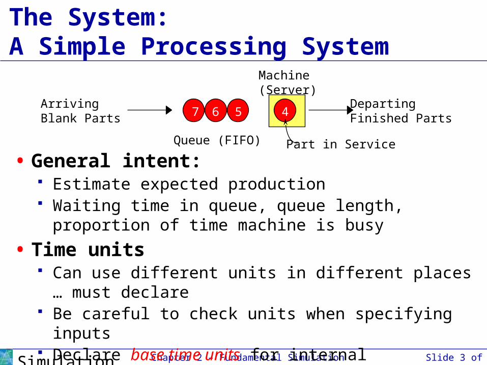
The System:A Simple Processing System
ArrivingBlank Parts
DepartingFinished Parts
Machine(Server)
Queue (FIFO) Part in Service
4567
• General intent: Estimate expected production Waiting time in queue, queue length, proportion of time
machine is busy
• Time units Can use different units in different places … must declare Be careful to check units when specifying inputs Declare base time units for internal calculations, outputs Be reasonable (interpretation, roundoff error)

Chapter 2 – Fundamental Simulation Concepts Slide 4 of 57Simulation with Arena, 5th ed.
Model Specifics
• Initially (time 0) empty and idle• Base time units: minutes• Input data (assume given for now …), in minutes:
Part Number Arrival Time Interarrival Time Service Time1 0.00 1.73 2.902 1.73 1.35 1.763 3.08 0.71 3.394 3.79 0.62 4.525 4.41 14.28 4.466 18.69 0.70 4.367 19.39 15.52 2.078 34.91 3.15 3.369 38.06 1.76 2.37
10 39.82 1.00 5.3811 40.82 . .
. . . .
. . . .
• Stop when 20 minutes of (simulated) time have passed
Chapter 2 – Fundamental Simulation Concepts Slide 5 of 57Simulation with Arena, 5th ed.
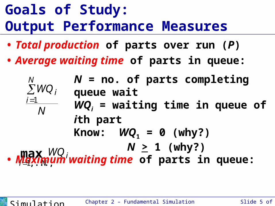
Goals of Study:Output Performance Measures• Total production of parts over run (P)
• Average waiting time of parts in queue:
• Maximum waiting time of parts in queue:
N = no. of parts completing queue waitWQi = waiting time in queue of ith partKnow: WQ1 = 0 (why?)
N > 1 (why?)N
WQN
ii
1
iNi
WQmax,...,1
Chapter 2 – Fundamental Simulation Concepts Slide 6 of 57Simulation with Arena, 5th ed.
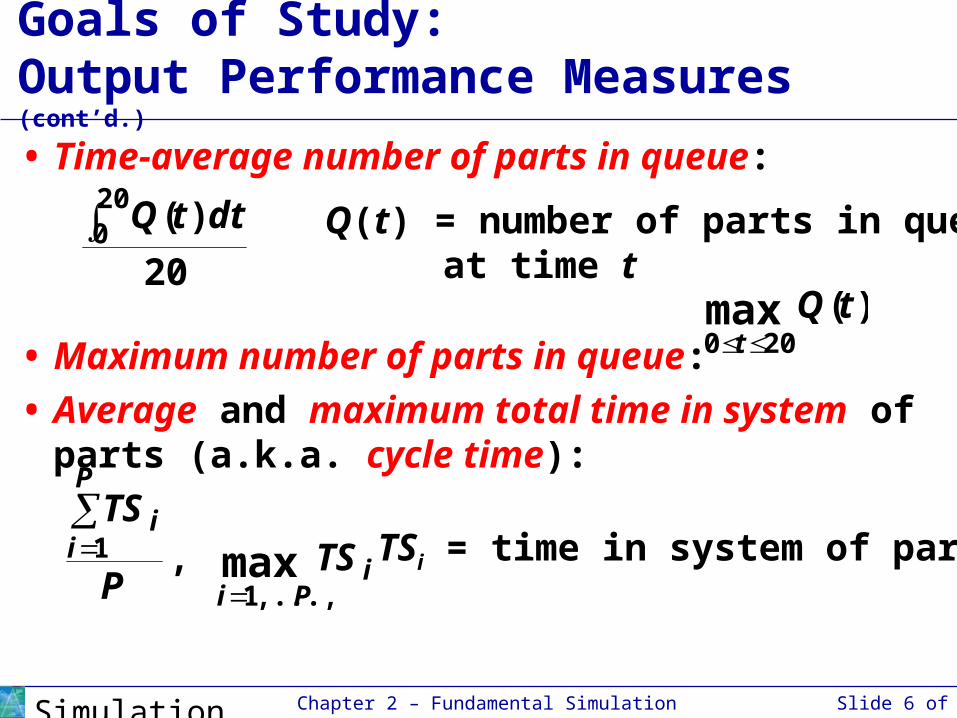
Goals of Study:Output Performance Measures (cont’d.)
• Time-average number of parts in queue:
• Maximum number of parts in queue:
• Average and maximum total time in system of parts (a.k.a. cycle time):
Q(t) = number of parts in queue at time t20
)(200 dttQ
)(max200
tQt
iPi
P
ii
TSP
TS
max,...,1
1 ,
TSi = time in system of part i
Chapter 2 – Fundamental Simulation Concepts Slide 7 of 57Simulation with Arena, 5th ed.
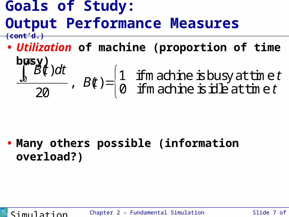
Goals of Study:Output Performance Measures (cont’d.)
• Utilization of machine (proportion of time busy)
• Many others possible (information overload?)
20
0( ) 1 if machine is busy at time , ( ) 0 if machine is idle at time 20
B t dt tB t t
Chapter 2 – Fundamental Simulation Concepts Slide 8 of 57Simulation with Arena, 5th ed.
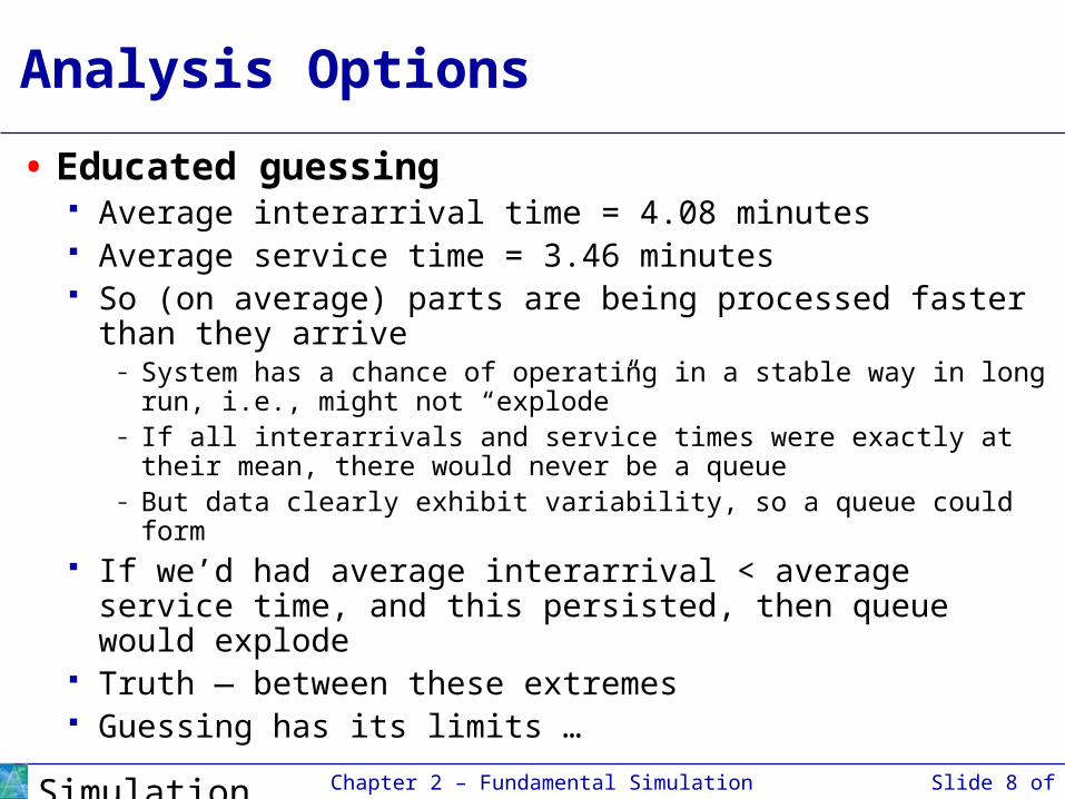
Analysis Options
• Educated guessing Average interarrival time = 4.08 minutes Average service time = 3.46 minutes So (on average) parts are being processed faster than they
arrive– System has a chance of operating in a stable way in long run, i.e.,
might not “explode”– If all interarrivals and service times were exactly at their mean,
there would never be a queue– But data clearly exhibit variability, so a queue could form
If we’d had average interarrival < average service time, and this persisted, then queue would explode
Truth — between these extremes Guessing has its limits …

Chapter 2 – Fundamental Simulation Concepts Slide 9 of 57Simulation with Arena, 5th ed.
Analysis Options (cont’d.)
• Queueing theory Requires additional assumptions about model Popular, simple model: M/M/1 queue
– Interarrival times ~ exponential– Service times ~ exponential, indep. of interarrivals– Must have E(service) < E(interarrival)– Steady-state (long-run, forever)– Exact analytic results; e.g., average waiting time in queue is
Problems: validity, estimating means, time frame Often useful as first-cut approximation
time) E(service
time) ivalE(interarr 2
S
A
SA
S
,

Chapter 2 – Fundamental Simulation Concepts Slide 10 of 57Simulation with Arena, 5th ed.
Mechanistic Simulation
• Individual operations (arrivals, service times) will occur exactly as in reality
• Movements, changes occur at right “times,” in right order
• Different pieces interact
• Install “observers” to get output performance measures
• Concrete, “brute-force” analysis approach
• Nothing mysterious or subtle But a lot of details, bookkeeping Simulation software keeps track of things for you
Chapter 2 – Fundamental Simulation Concepts Slide 11 of 57Simulation with Arena, 5th ed.
Pieces of a Simulation Model
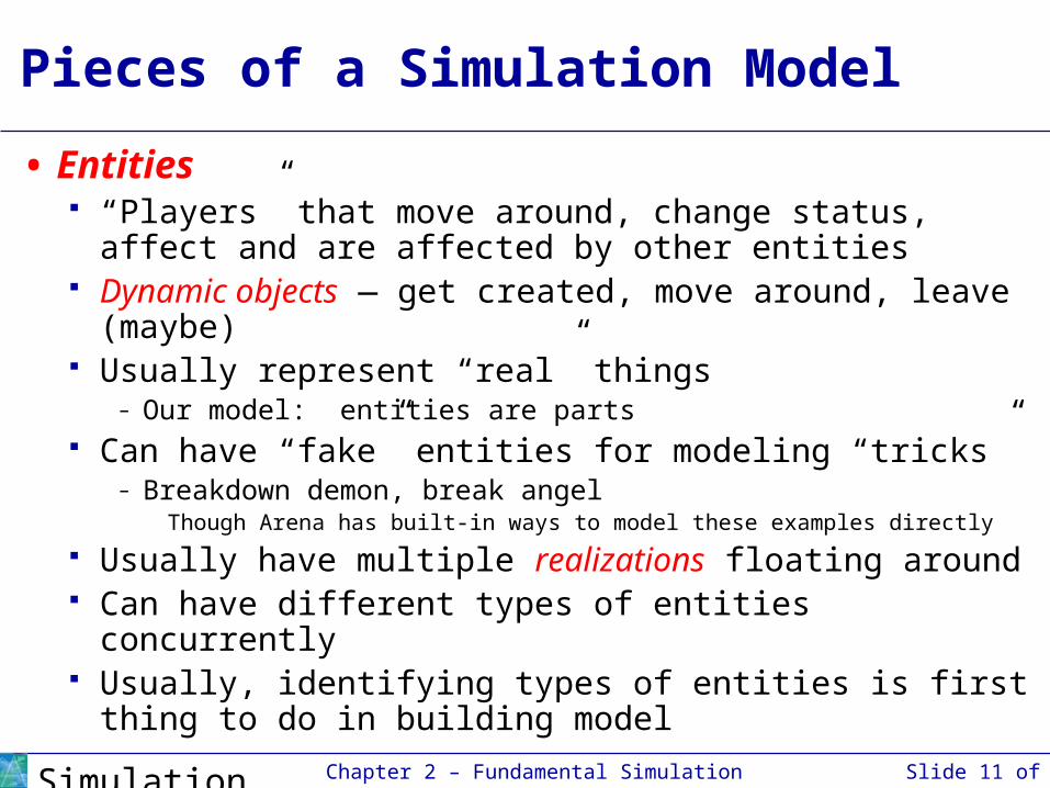
• Entities “Players” that move around, change status, affect and are
affected by other entities Dynamic objects — get created, move around, leave
(maybe) Usually represent “real” things
– Our model: entities are parts Can have “fake” entities for modeling “tricks”
– Breakdown demon, break angelThough Arena has built-in ways to model these examples directly
Usually have multiple realizations floating around Can have different types of entities concurrently Usually, identifying types of entities is first thing to do in
building model

Chapter 2 – Fundamental Simulation Concepts Slide 12 of 57Simulation with Arena, 5th ed.
Pieces of a Simulation Model (cont’d.)
• Attributes Characteristic of all entities: describe, differentiate All entities have same attribute “slots” but different values
for different entities, for example:– Time of arrival– Due date– Priority– Color
Attribute value tied to a specific entity Like “local” (to entities) variables Some automatic in Arena, some you define
Chapter 2 – Fundamental Simulation Concepts Slide 13 of 57Simulation with Arena, 5th ed.
Pieces of a Simulation Model (cont’d.)
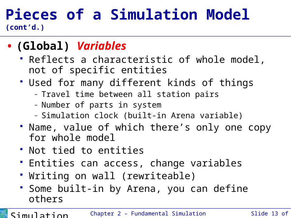
• (Global) Variables Reflects a characteristic of whole model, not of specific
entities Used for many different kinds of things
– Travel time between all station pairs– Number of parts in system– Simulation clock (built-in Arena variable)
Name, value of which there’s only one copy for whole model
Not tied to entities Entities can access, change variables Writing on wall (rewriteable) Some built-in by Arena, you can define others
Chapter 2 – Fundamental Simulation Concepts Slide 14 of 57Simulation with Arena, 5th ed.
Pieces of a Simulation Model (cont’d.)
• Resources What entities compete for
– People– Equipment– Space
Entity seizes a resource, uses it, releases it Think of a resource being assigned to an entity, rather than
an entity “belonging to” a resource “A” resource can have several units of capacity
– Seats at a table in a restaurant– Identical ticketing agents at an airline counter
Number of units of resource can be changed during simulation
Chapter 2 – Fundamental Simulation Concepts Slide 15 of 57Simulation with Arena, 5th ed.
Pieces of a Simulation Model (cont’d.)
• Queues Place for entities to wait when they can’t move on (maybe
since resource they want to seize is not available) Have names, often tied to a corresponding resource Can have a finite capacity to model limited space — have
to model what to do if an entity shows up to a queue that’s already full
Usually watch length of a queue, waiting time in it
Chapter 2 – Fundamental Simulation Concepts Slide 16 of 57Simulation with Arena, 5th ed.
Pieces of a Simulation Model (cont’d.)
• Statistical accumulators Variables that “watch” what’s happening Depend on output performance measures desired “Passive” in model — don’t participate, just watch Many are automatic in Arena, but some you may have to
set up and maintain during simulation At end of simulation, used to compute final output
performance measures
Chapter 2 – Fundamental Simulation Concepts Slide 17 of 57Simulation with Arena, 5th ed.
Pieces of a Simulation Model (cont’d.)
• Statistical accumulators for simple processing system Number of parts produced so far Total of waiting times spent in queue so far No. of parts that have gone through queue Max time in queue we’ve seen so far Total of times spent in system Max time in system we’ve seen so far Area so far under queue-length curve Q(t) Max of Q(t) so far Area so far under server-busy curve B(t)
Chapter 2 – Fundamental Simulation Concepts Slide 18 of 57Simulation with Arena, 5th ed.
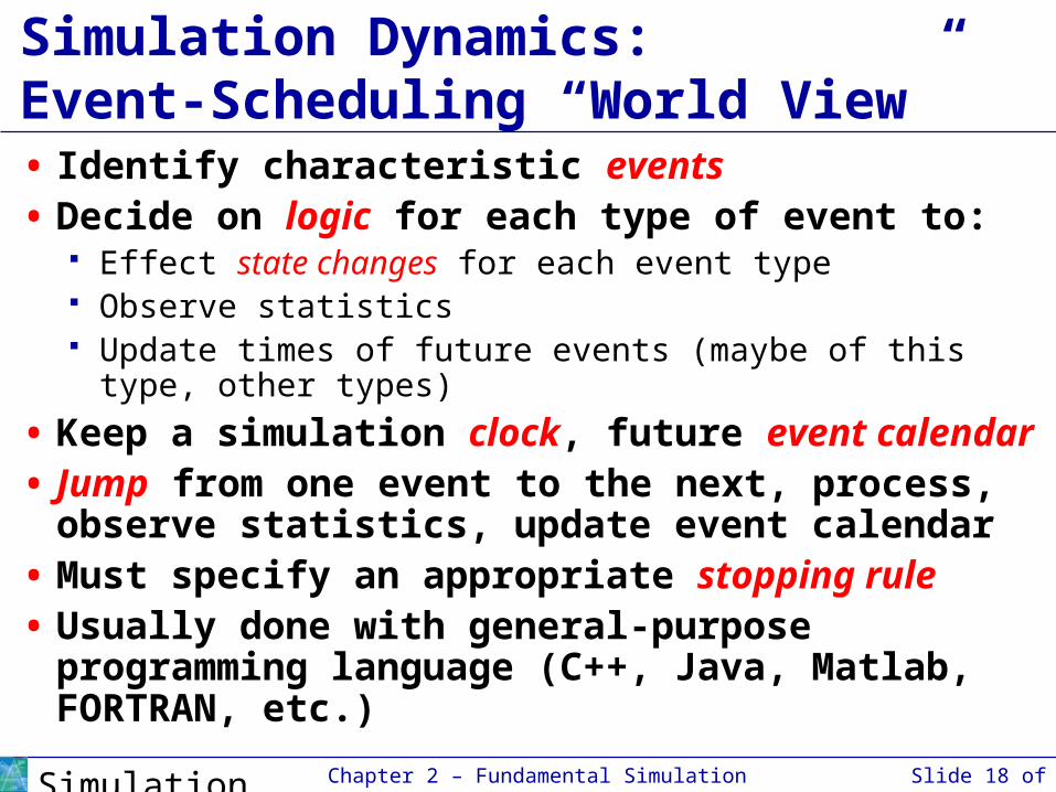
Simulation Dynamics:Event-Scheduling “World View”• Identify characteristic events• Decide on logic for each type of event to:
Effect state changes for each event type Observe statistics Update times of future events (maybe of this type, other
types)
• Keep a simulation clock, future event calendar• Jump from one event to the next, process,
observe statistics, update event calendar• Must specify an appropriate stopping rule• Usually done with general-purpose programming
language (C++, Java, Matlab, FORTRAN, etc.)

Chapter 2 – Fundamental Simulation Concepts Slide 19 of 57Simulation with Arena, 5th ed.
Events for theSimple Processing System• Arrival of a new part to system
Update time-persistent statistical accumulators (from last event to now)
– Area under Q(t)– Max of Q(t)– Area under B(t)
“Mark” arriving part with current time (use later) If machine is idle:
– Start processing (schedule departure), Make machine busy, Tally waiting time in queue (0)
Else (machine is busy):– Put part at end of queue, increase queue-length variable
Schedule next arrival event
Chapter 2 – Fundamental Simulation Concepts Slide 20 of 57Simulation with Arena, 5th ed.
Events for theSimple Processing System (cont’d.)
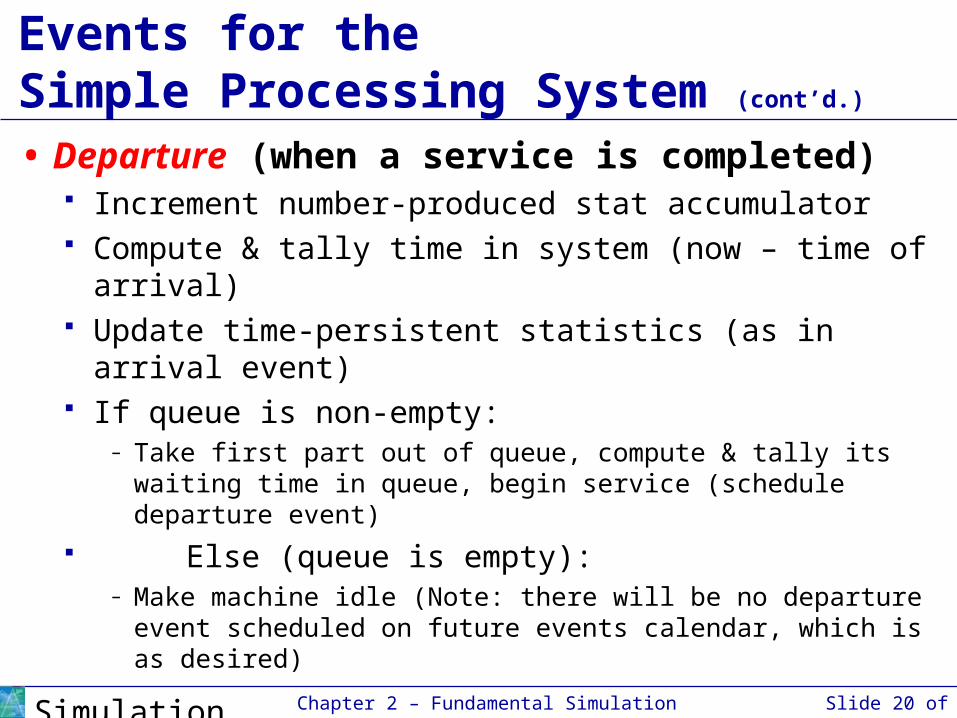
• Departure (when a service is completed) Increment number-produced stat accumulator Compute & tally time in system (now – time of arrival) Update time-persistent statistics (as in arrival event) If queue is non-empty:
– Take first part out of queue, compute & tally its waiting time in queue, begin service (schedule departure event)
Else (queue is empty):– Make machine idle (Note: there will be no departure event
scheduled on future events calendar, which is as desired)
Chapter 2 – Fundamental Simulation Concepts Slide 21 of 57Simulation with Arena, 5th ed.
Events for theSimple Processing System (cont’d.)
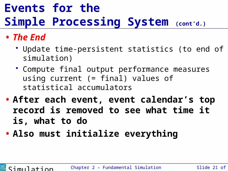
• The End Update time-persistent statistics (to end of simulation) Compute final output performance measures using current
(= final) values of statistical accumulators
• After each event, event calendar’s top record is removed to see what time it is, what to do
• Also must initialize everything
Chapter 2 – Fundamental Simulation Concepts Slide 22 of 57Simulation with Arena, 5th ed.
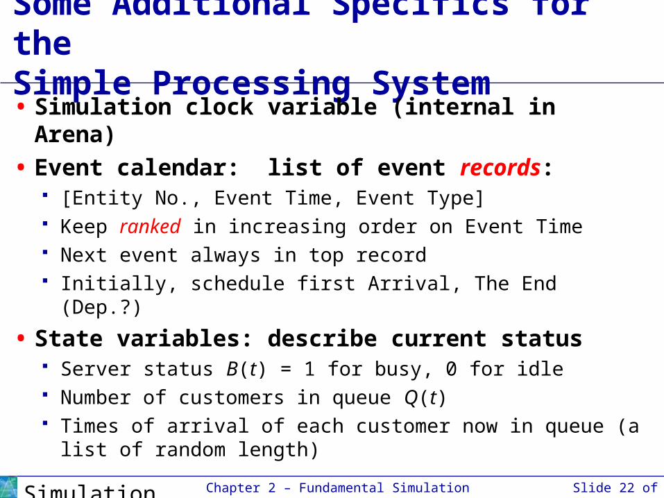
Some Additional Specifics for theSimple Processing System• Simulation clock variable (internal in Arena)
• Event calendar: list of event records: [Entity No., Event Time, Event Type] Keep ranked in increasing order on Event Time Next event always in top record Initially, schedule first Arrival, The End (Dep.?)
• State variables: describe current status Server status B(t) = 1 for busy, 0 for idle Number of customers in queue Q(t) Times of arrival of each customer now in queue (a list of
random length)

Chapter 2 – Fundamental Simulation Concepts Slide 23 of 57Simulation with Arena, 5th ed.
Simulation by Hand
• Manually track state variables, statistical accumulators
• Use “given” interarrival, service times
• Keep track of event calendar
• “Lurch” clock from one event to next
• Will omit times in system, “max” computations here (see text for complete details)

Chapter 2 – Fundamental Simulation Concepts Slide 24 of 57Simulation with Arena, 5th ed.
System
Clock
B(t)
Q(t)
Arrival times of custs. in queue
Event calendar
Number of completed waiting times in queue
Total of waiting times in queue
Area under Q(t)
Area under B(t)
Q(t) graph B(t) graph
Time (Minutes) Interarrival times 1.73, 1.35, 0.71, 0.62, 14.28, 0.70, 15.52, 3.15, 1.76, 1.00, ...
Service times 2.90, 1.76, 3.39, 4.52, 4.46, 4.36, 2.07, 3.36, 2.37, 5.38, ...
Simulation by Hand:Setup
0
1
2
3
4
0 5 10 15 20
012
0 5 10 15 20
Chapter 2 – Fundamental Simulation Concepts Slide 25 of 57Simulation with Arena, 5th ed.
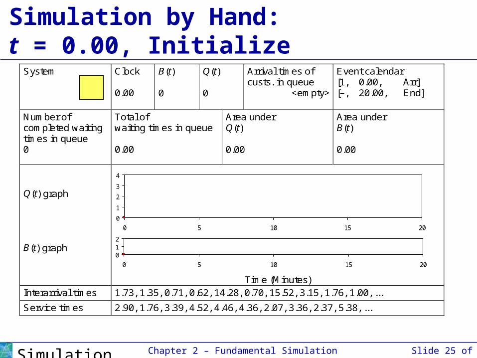
System
Clock 0.00
B(t) 0
Q(t) 0
Arrival times of custs. in queue
<empty>
Event calendar [1, 0.00, Arr] [–, 20.00, End]
Number of completed waiting times in queue 0
Total of waiting times in queue 0.00
Area under Q(t) 0.00
Area under B(t) 0.00
Q(t) graph B(t) graph
Time (Minutes) Interarrival times 1.73, 1.35, 0.71, 0.62, 14.28, 0.70, 15.52, 3.15, 1.76, 1.00, ...
Service times 2.90, 1.76, 3.39, 4.52, 4.46, 4.36, 2.07, 3.36, 2.37, 5.38, ...
Simulation by Hand:t = 0.00, Initialize
0
1
2
3
4
0 5 10 15 20
012
0 5 10 15 20
Chapter 2 – Fundamental Simulation Concepts Slide 26 of 57Simulation with Arena, 5th ed.
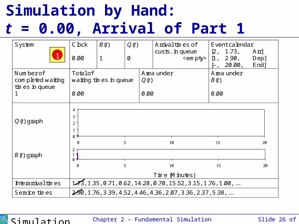
System
Clock 0.00
B(t) 1
Q(t) 0
Arrival times of custs. in queue
<empty>
Event calendar [2, 1.73, Arr] [1, 2.90, Dep] [–, 20.00, End]
Number of completed waiting times in queue 1
Total of waiting times in queue 0.00
Area under Q(t) 0.00
Area under B(t) 0.00
Q(t) graph B(t) graph
Time (Minutes) Interarrival times 1.73, 1.35, 0.71, 0.62, 14.28, 0.70, 15.52, 3.15, 1.76, 1.00, ...
Service times 2.90, 1.76, 3.39, 4.52, 4.46, 4.36, 2.07, 3.36, 2.37, 5.38, ...
Simulation by Hand:t = 0.00, Arrival of Part 1
0
1
2
3
4
0 5 10 15 20
012
0 5 10 15 20
1
Chapter 2 – Fundamental Simulation Concepts Slide 27 of 57Simulation with Arena, 5th ed.
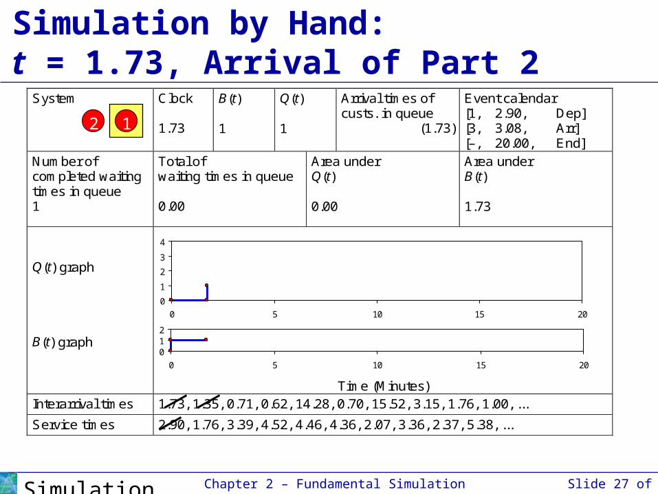
System
Clock 1.73
B(t) 1
Q(t) 1
Arrival times of custs. in queue
(1.73)
Event calendar [1, 2.90, Dep] [3, 3.08, Arr] [–, 20.00, End]
Number of completed waiting times in queue 1
Total of waiting times in queue 0.00
Area under Q(t) 0.00
Area under B(t) 1.73
Q(t) graph B(t) graph
Time (Minutes) Interarrival times 1.73, 1.35, 0.71, 0.62, 14.28, 0.70, 15.52, 3.15, 1.76, 1.00, ...
Service times 2.90, 1.76, 3.39, 4.52, 4.46, 4.36, 2.07, 3.36, 2.37, 5.38, ...
Simulation by Hand:t = 1.73, Arrival of Part 2
0
1
2
3
4
0 5 10 15 20
012
0 5 10 15 20
12
Chapter 2 – Fundamental Simulation Concepts Slide 28 of 57Simulation with Arena, 5th ed.
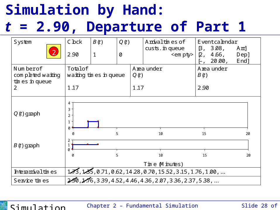
System
Clock 2.90
B(t) 1
Q(t) 0
Arrival times of custs. in queue
<empty>
Event calendar [3, 3.08, Arr] [2, 4.66, Dep] [–, 20.00, End]
Number of completed waiting times in queue 2
Total of waiting times in queue 1.17
Area under Q(t) 1.17
Area under B(t) 2.90
Q(t) graph B(t) graph
Time (Minutes) Interarrival times 1.73, 1.35, 0.71, 0.62, 14.28, 0.70, 15.52, 3.15, 1.76, 1.00, ...
Service times 2.90, 1.76, 3.39, 4.52, 4.46, 4.36, 2.07, 3.36, 2.37, 5.38, ...
Simulation by Hand:t = 2.90, Departure of Part 1
0
1
2
3
4
0 5 10 15 20
012
0 5 10 15 20
2
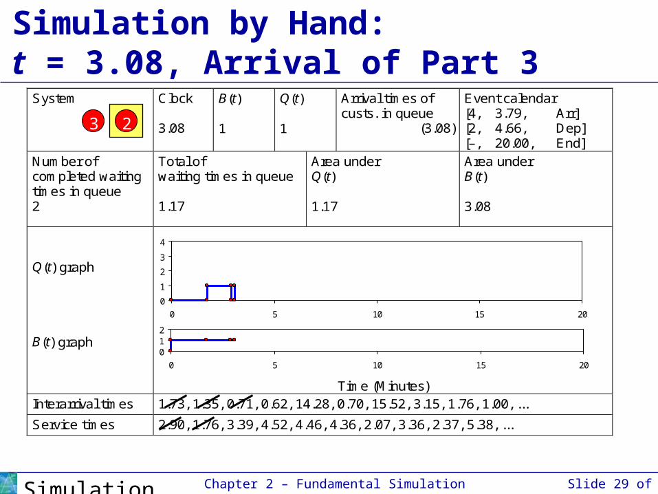
Chapter 2 – Fundamental Simulation Concepts Slide 29 of 57Simulation with Arena, 5th ed.
System
Clock 3.08
B(t) 1
Q(t) 1
Arrival times of custs. in queue
(3.08)
Event calendar [4, 3.79, Arr] [2, 4.66, Dep] [–, 20.00, End]
Number of completed waiting times in queue 2
Total of waiting times in queue 1.17
Area under Q(t) 1.17
Area under B(t) 3.08
Q(t) graph B(t) graph
Time (Minutes) Interarrival times 1.73, 1.35, 0.71, 0.62, 14.28, 0.70, 15.52, 3.15, 1.76, 1.00, ...
Service times 2.90, 1.76, 3.39, 4.52, 4.46, 4.36, 2.07, 3.36, 2.37, 5.38, ...
Simulation by Hand:t = 3.08, Arrival of Part 3
0
1
2
3
4
0 5 10 15 20
012
0 5 10 15 20
23

Chapter 2 – Fundamental Simulation Concepts Slide 30 of 57Simulation with Arena, 5th ed.
System
Clock 3.79
B(t) 1
Q(t) 2
Arrival times of custs. in queue
(3.79, 3.08)
Event calendar [5, 4.41, Arr] [2, 4.66, Dep] [–, 20.00, End]
Number of completed waiting times in queue 2
Total of waiting times in queue 1.17
Area under Q(t) 1.88
Area under B(t) 3.79
Q(t) graph B(t) graph
Time (Minutes) Interarrival times 1.73, 1.35, 0.71, 0.62, 14.28, 0.70, 15.52, 3.15, 1.76, 1.00, ...
Service times 2.90, 1.76, 3.39, 4.52, 4.46, 4.36, 2.07, 3.36, 2.37, 5.38, ...
Simulation by Hand:t = 3.79, Arrival of Part 4
0
1
2
3
4
0 5 10 15 20
012
0 5 10 15 20
234
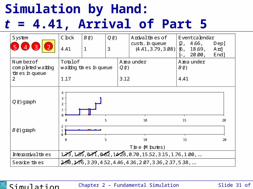
Chapter 2 – Fundamental Simulation Concepts Slide 31 of 57Simulation with Arena, 5th ed.
System
Clock 4.41
B(t) 1
Q(t) 3
Arrival times of custs. in queue
(4.41, 3.79, 3.08)
Event calendar [2, 4.66, Dep] [6, 18.69, Arr] [–, 20.00, End]
Number of completed waiting times in queue 2
Total of waiting times in queue 1.17
Area under Q(t) 3.12
Area under B(t) 4.41
Q(t) graph B(t) graph
Time (Minutes)
Interarrival times 1.73, 1.35, 0.71, 0.62, 14.28, 0.70, 15.52, 3.15, 1.76, 1.00, ...
Service times 2.90, 1.76, 3.39, 4.52, 4.46, 4.36, 2.07, 3.36, 2.37, 5.38, ...
Simulation by Hand:t = 4.41, Arrival of Part 5
0
1
2
3
4
0 5 10 15 20
012
0 5 10 15 20
2345
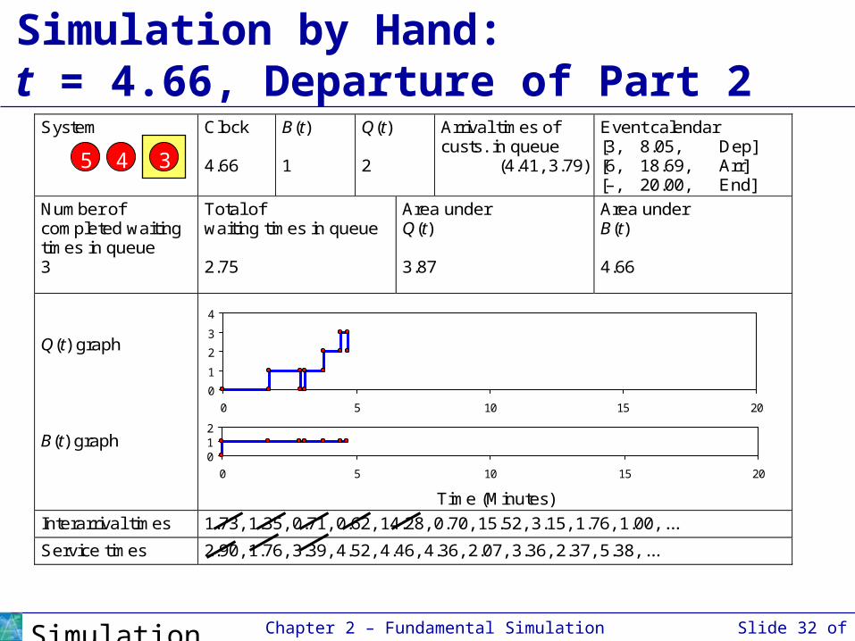
Chapter 2 – Fundamental Simulation Concepts Slide 32 of 57Simulation with Arena, 5th ed.
System
Clock 4.66
B(t) 1
Q(t) 2
Arrival times of custs. in queue
(4.41, 3.79)
Event calendar [3, 8.05, Dep] [6, 18.69, Arr] [–, 20.00, End]
Number of completed waiting times in queue 3
Total of waiting times in queue 2.75
Area under Q(t) 3.87
Area under B(t) 4.66
Q(t) graph B(t) graph
Time (Minutes)
Interarrival times 1.73, 1.35, 0.71, 0.62, 14.28, 0.70, 15.52, 3.15, 1.76, 1.00, ...
Service times 2.90, 1.76, 3.39, 4.52, 4.46, 4.36, 2.07, 3.36, 2.37, 5.38, ...
Simulation by Hand:t = 4.66, Departure of Part 2
0
1
2
3
4
0 5 10 15 20
012
0 5 10 15 20
345
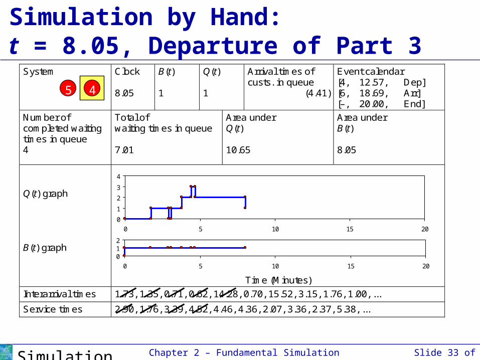
Chapter 2 – Fundamental Simulation Concepts Slide 33 of 57Simulation with Arena, 5th ed.
System
Clock 8.05
B(t) 1
Q(t) 1
Arrival times of custs. in queue
(4.41)
Event calendar [4, 12.57, Dep] [6, 18.69, Arr] [–, 20.00, End]
Number of completed waiting times in queue 4
Total of waiting times in queue 7.01
Area under Q(t) 10.65
Area under B(t) 8.05
Q(t) graph B(t) graph
Time (Minutes)
Interarrival times 1.73, 1.35, 0.71, 0.62, 14.28, 0.70, 15.52, 3.15, 1.76, 1.00, ...
Service times 2.90, 1.76, 3.39, 4.52, 4.46, 4.36, 2.07, 3.36, 2.37, 5.38, ...
Simulation by Hand:t = 8.05, Departure of Part 3
0
1
2
3
4
0 5 10 15 20
012
0 5 10 15 20
45
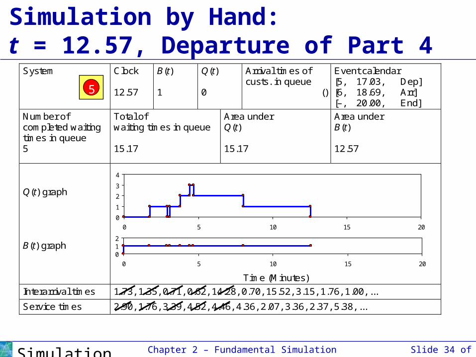
Chapter 2 – Fundamental Simulation Concepts Slide 34 of 57Simulation with Arena, 5th ed.
System
Clock 12.57
B(t) 1
Q(t) 0
Arrival times of custs. in queue
()
Event calendar [5, 17.03, Dep] [6, 18.69, Arr] [–, 20.00, End]
Number of completed waiting times in queue 5
Total of waiting times in queue 15.17
Area under Q(t) 15.17
Area under B(t) 12.57
Q(t) graph B(t) graph
Time (Minutes)
Interarrival times 1.73, 1.35, 0.71, 0.62, 14.28, 0.70, 15.52, 3.15, 1.76, 1.00, ...
Service times 2.90, 1.76, 3.39, 4.52, 4.46, 4.36, 2.07, 3.36, 2.37, 5.38, ...
Simulation by Hand:t = 12.57, Departure of Part 4
0
1
2
3
4
0 5 10 15 20
012
0 5 10 15 20
5
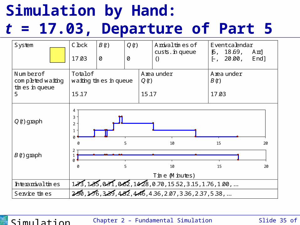
Chapter 2 – Fundamental Simulation Concepts Slide 35 of 57Simulation with Arena, 5th ed.
System
Clock 17.03
B(t) 0
Q(t) 0
Arrival times of custs. in queue ()
Event calendar [6, 18.69, Arr] [–, 20.00, End]
Number of completed waiting times in queue 5
Total of waiting times in queue 15.17
Area under Q(t) 15.17
Area under B(t) 17.03
Q(t) graph B(t) graph
Time (Minutes)
Interarrival times 1.73, 1.35, 0.71, 0.62, 14.28, 0.70, 15.52, 3.15, 1.76, 1.00, ...
Service times 2.90, 1.76, 3.39, 4.52, 4.46, 4.36, 2.07, 3.36, 2.37, 5.38, ...
Simulation by Hand:t = 17.03, Departure of Part 5
0
1
2
3
4
0 5 10 15 20
012
0 5 10 15 20

Chapter 2 – Fundamental Simulation Concepts Slide 36 of 57Simulation with Arena, 5th ed.
System
Clock 18.69
B(t) 1
Q(t) 0
Arrival times of custs. in queue ()
Event calendar [7, 19.39, Arr] [–, 20.00, End] [6, 23.05, Dep]
Number of completed waiting times in queue 6
Total of waiting times in queue 15.17
Area under Q(t) 15.17
Area under B(t) 17.03
Q(t) graph B(t) graph
Time (Minutes)
Interarrival times 1.73, 1.35, 0.71, 0.62, 14.28, 0.70, 15.52, 3.15, 1.76, 1.00, ...
Service times 2.90, 1.76, 3.39, 4.52, 4.46, 4.36, 2.07, 3.36, 2.37, 5.38, ...
Simulation by Hand:t = 18.69, Arrival of Part 6
0
1
2
3
4
0 5 10 15 20
012
0 5 10 15 20
6

Chapter 2 – Fundamental Simulation Concepts Slide 37 of 57Simulation with Arena, 5th ed.
System
Clock 19.39
B(t) 1
Q(t) 1
Arrival times of custs. in queue
(19.39)
Event calendar [–, 20.00, End] [6, 23.05, Dep] [8, 34.91, Arr]
Number of completed waiting times in queue 6
Total of waiting times in queue 15.17
Area under Q(t) 15.17
Area under B(t) 17.73
Q(t) graph B(t) graph
Time (Minutes)
Interarrival times 1.73, 1.35, 0.71, 0.62, 14.28, 0.70, 15.52, 3.15, 1.76, 1.00, ...
Service times 2.90, 1.76, 3.39, 4.52, 4.46, 4.36, 2.07, 3.36, 2.37, 5.38, ...
Simulation by Hand:t = 19.39, Arrival of Part 7
0
1
2
3
4
0 5 10 15 20
012
0 5 10 15 20
67
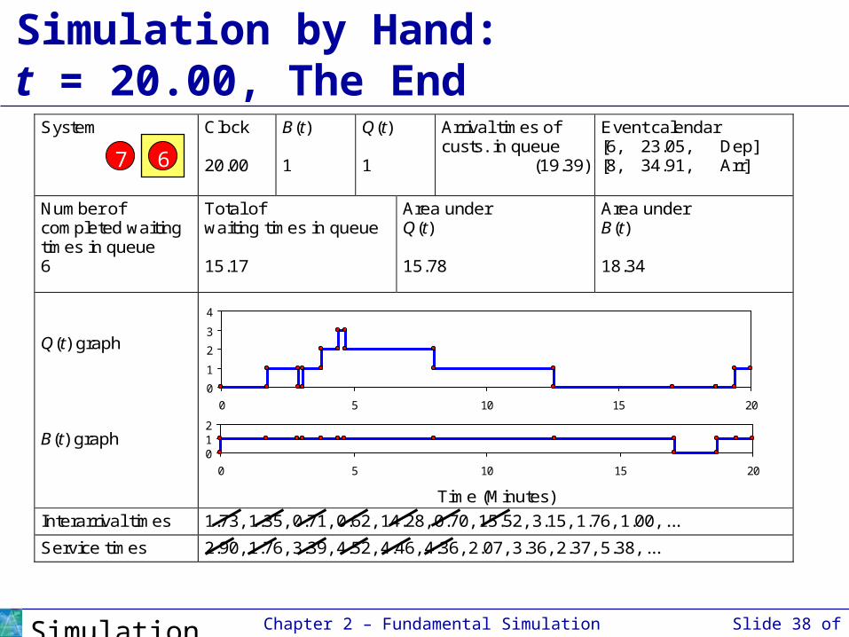
Chapter 2 – Fundamental Simulation Concepts Slide 38 of 57Simulation with Arena, 5th ed.
Simulation by Hand:t = 20.00, The End
0
1
2
3
4
0 5 10 15 20
012
0 5 10 15 20
67
System
Clock 20.00
B(t) 1
Q(t) 1
Arrival times of custs. in queue
(19.39)
Event calendar [6, 23.05, Dep] [8, 34.91, Arr]
Number of completed waiting times in queue 6
Total of waiting times in queue 15.17
Area under Q(t) 15.78
Area under B(t) 18.34
Q(t) graph B(t) graph
Time (Minutes)
Interarrival times 1.73, 1.35, 0.71, 0.62, 14.28, 0.70, 15.52, 3.15, 1.76, 1.00, ...
Service times 2.90, 1.76, 3.39, 4.52, 4.46, 4.36, 2.07, 3.36, 2.37, 5.38, ...

Chapter 2 – Fundamental Simulation Concepts Slide 39 of 57Simulation with Arena, 5th ed.
Simulation by Hand:Finishing Up• Average waiting time in queue:
• Time-average number in queue:
• Utilization of drill press:
part per minutes 53261715
queue in times of No.queue in times of Total
..
part 79020
7815value clock Final
curve under Area.
.)( tQ
less)(dimension 92020
3418value clock Final
curve under Area.
.)( tB
Chapter 2 – Fundamental Simulation Concepts Slide 40 of 57Simulation with Arena, 5th ed.
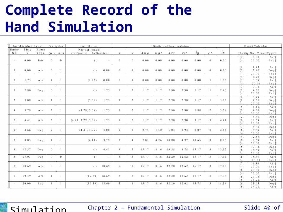
Complete Record of theHand Simulation
Chapter 2 – Fundamental Simulation Concepts Slide 41 of 57Simulation with Arena, 5th ed.
Event-Scheduling Logic via Programming• Clearly well suited to standard programming
language (C, C++, Java, etc.)
• Often use “utility” libraries for: List processing Random-number generation Random-variate generation Statistics collection Event-list and clock management Summary and output
• Main program ties it together, executes events in order

Chapter 2 – Fundamental Simulation Concepts Slide 42 of 57Simulation with Arena, 5th ed.
Simulation Dynamics:Process-Interaction World View• Identify characteristic entities in system• Multiple copies of entities co-exist, interact,
compete• “Code” is non-procedural• Tell a “story” about what happens to a “typical”
entity• May have many types of entities, “fake” entities
for things like machine breakdowns• Usually requires special simulation software
Underneath, still executed as event-scheduling
• View normally taken by Arena Arena translates your model description into a program in
SIMAN simulation language for execution
Chapter 2 – Fundamental Simulation Concepts Slide 43 of 57Simulation with Arena, 5th ed.
Randomness in Simulation
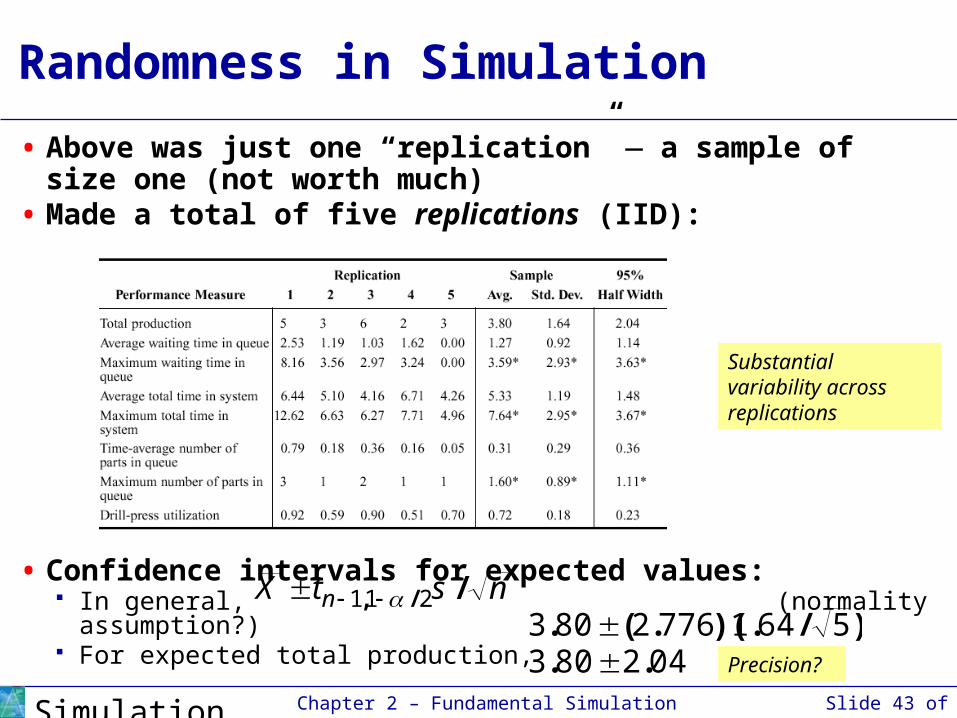
• Above was just one “replication” — a sample of size one (not worth much)
• Made a total of five replications (IID):
• Confidence intervals for expected values: In general, (normality assumption?) For expected total production,
nstX n //, 211 )/.)(.(. 56417762803
042803 ..
Substantial variability across replications
Precision?

Chapter 2 – Fundamental Simulation Concepts Slide 44 of 57Simulation with Arena, 5th ed.
Comparing Alternatives
• Usually, simulation is used for more than just a single model “configuration”
• Often want to compare alternatives, select or search for best (via some criterion)
• Simple processing system: What would happen if arrival rate doubled? Cut interarrival times in half Rerun model for double-time arrivals Make five replications
Chapter 2 – Fundamental Simulation Concepts Slide 45 of 57Simulation with Arena, 5th ed.
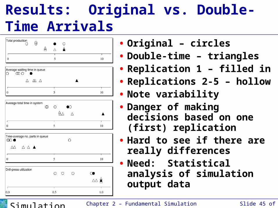
Results: Original vs. Double-Time Arrivals
• Original – circles• Double-time – triangles• Replication 1 – filled in• Replications 2-5 – hollow• Note variability• Danger of making decisions
based on one (first) replication
• Hard to see if there are really differences
• Need: Statistical analysis of simulation output data
Chapter 2 – Fundamental Simulation Concepts Slide 46 of 57Simulation with Arena, 5th ed.
Simulating with Spreadsheets:Introduction• Popular, ubiquitous tool
• Can use for simple simulation models Typically, only static models
– Risk analysis, financial/investment scenarios
Only (very) simplest of dynamic models
• Two examples Newsvendor problem (static) Waiting times in single-server queue (dynamic)
– Special recursion valid only in this case
Chapter 2 – Fundamental Simulation Concepts Slide 47 of 57Simulation with Arena, 5th ed.
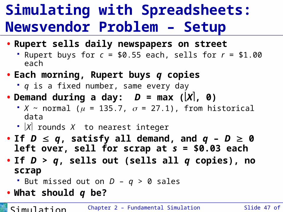
Simulating with Spreadsheets:Newsvendor Problem – Setup• Rupert sells daily newspapers on street
Rupert buys for c = $0.55 each, sells for r = $1.00 each
• Each morning, Rupert buys q copies q is a fixed number, same every day
• Demand during a day: D = max (X, 0) X ~ normal ( = 135.7, = 27.1), from historical data X rounds X to nearest integer
• If D q, satisfy all demand, and q – D 0 left over, sell for scrap at s = $0.03 each
• If D > q, sells out (sells all q copies), no scrap But missed out on D – q > 0 sales
• What should q be?
Chapter 2 – Fundamental Simulation Concepts Slide 48 of 57Simulation with Arena, 5th ed.
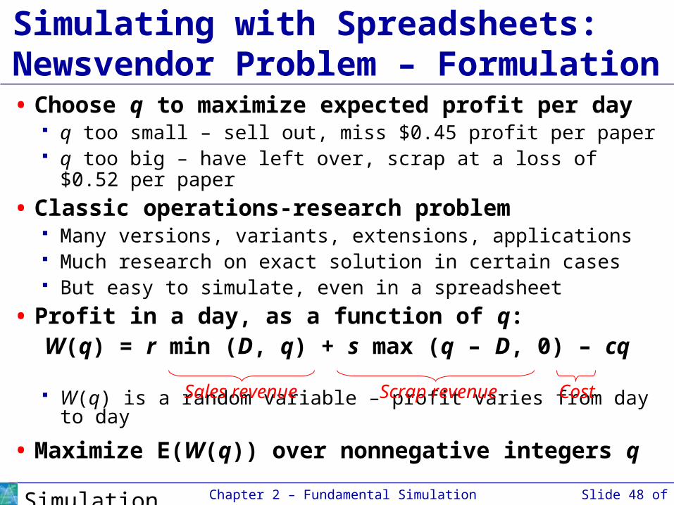
Simulating with Spreadsheets:Newsvendor Problem – Formulation• Choose q to maximize expected profit per day
q too small – sell out, miss $0.45 profit per paper q too big – have left over, scrap at a loss of $0.52 per paper
• Classic operations-research problem Many versions, variants, extensions, applications Much research on exact solution in certain cases But easy to simulate, even in a spreadsheet
• Profit in a day, as a function of q:W(q) = r min (D, q) + s max (q – D, 0) – cq
W(q) is a random variable – profit varies from day to day
• Maximize E(W(q)) over nonnegative integers q
Sales revenue Scrap revenue Cost
Chapter 2 – Fundamental Simulation Concepts Slide 49 of 57Simulation with Arena, 5th ed.
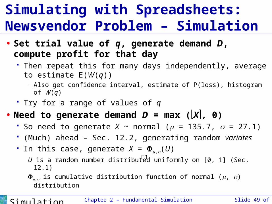
Simulating with Spreadsheets:Newsvendor Problem – Simulation• Set trial value of q, generate demand D, compute
profit for that day Then repeat this for many days independently, average to
estimate E(W(q))– Also get confidence interval, estimate of P(loss), histogram of W(q)
Try for a range of values of q
• Need to generate demand D = max (X, 0) So need to generate X ~ normal ( = 135.7, = 27.1) (Much) ahead – Sec. 12.2, generating random variates In this case, generate X = ,(U)
U is a random number distributed uniformly on [0, 1] (Sec. 12.1)
, is cumulative distribution function of normal (, ) distribution
1
Chapter 2 – Fundamental Simulation Concepts Slide 50 of 57Simulation with Arena, 5th ed.
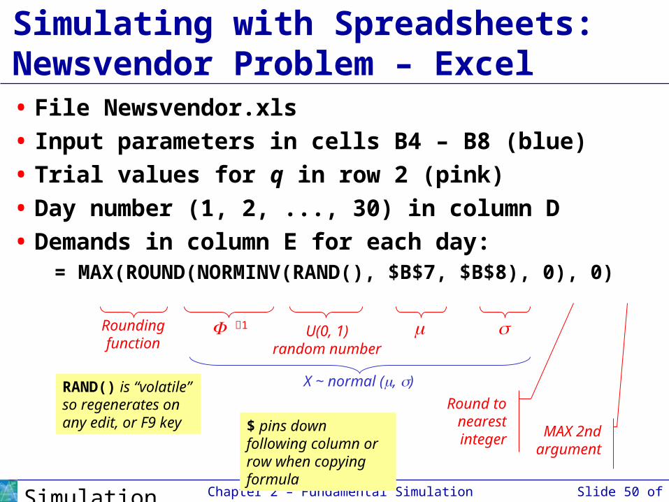
Simulating with Spreadsheets:Newsvendor Problem – Excel• File Newsvendor.xls
• Input parameters in cells B4 – B8 (blue)
• Trial values for q in row 2 (pink)
• Day number (1, 2, ..., 30) in column D
• Demands in column E for each day:= MAX(ROUND(NORMINV(RAND(), $B$7, $B$8), 0), 0)
Roundingfunction
1 U(0, 1)random number
X ~ normal (, )
Round to nearestinteger MAX 2nd
argument
$ pins down following column or row when copying formula
RAND() is “volatile” so regenerates on any edit, or F9 key
Chapter 2 – Fundamental Simulation Concepts Slide 51 of 57Simulation with Arena, 5th ed.
Simulating with Spreadsheets:Newsvendor Problem – Excel (cont’d.)
• For each q: “Sold” column: number of papers sold that day “Scrap” column: number of papers scrapped that day “Profit” column: profit (+, –, 0) that day Placement of “$” in formulas to facilitate copying
• At bottom of “Profit” columns (green): Average profit over 30 days Half-width of 95% confidence interval on E(W(q))
– Value 2.045 is upper 0.975 critical point of t distribution with 29 d.f.– Plot confidence intervals as “I-beams” on left edge
Estimate of P(W(q) < 0)– Uses COUNTIF function
• Histograms of W(q) at bottom Vertical red line at 0, separates profits, losses

Chapter 2 – Fundamental Simulation Concepts Slide 52 of 57Simulation with Arena, 5th ed.
Simulating with Spreadsheets:Newsvendor Problem – Results• Fine point – used same daily demands (column E)
for each day, across all trial values of q Would have been valid to generate them independently Why is it better to use same demands for all q?
• Results Best q is about 140, maybe a little less Randomness in all results (tap F9 key)
– All demands, profits, graphics change– Confidence-interval, histogram plots change– Reminder that these are random outputs, random plots
Higher q more variability in profit– Histograms at bottom are wider for larger q– Higher chance of both large profits, but higher chance of loss, too– Risk/return tradeoff can be quantified – risk taker vs. risk-averse
Chapter 2 – Fundamental Simulation Concepts Slide 53 of 57Simulation with Arena, 5th ed.
Simulating with Spreadsheets:Single-Server Queue – Setup• Like hand simulation, but:
Interarrival times ~ exponential with mean 1/ = 1.6 min. Service times ~ uniform on [a, b] = [0.27, 2.29] min. Stop when 50th waiting time in queue is observed
– i.e., when 50th customer begins service, not exits system
• Watch waiting times in queue WQ1, WQ2, ..., WQ50
Important – not watching anything else, unlike before
• Si = service time of customer i,Ai = interarrival time between custs. i – 1 and i
• Lindley’s recursion (1952): Initialize WQ1 = 0,
WQi = max (WQi – 1 + Si – 1 – Ai, 0), i = 2, 3, ...
Chapter 2 – Fundamental Simulation Concepts Slide 54 of 57Simulation with Arena, 5th ed.
Simulating with Spreadsheets:Single-Server Queue – Simulation• Need to generate random variates: let U ~ U[0, 1]
Exponential (mean 1/): Ai = –(1/) ln(1 – U) Uniform on [a, b]: Si = a + (b – a) U
• File MU1.xls• Input parameters in cells B4 – B6 (blue)
Some theoretical outputs in cells B8 – B10
• Customer number (i = 1, 2, ..., 50) in column D• Five IID replications (three columns for each)
IA = interarrival times, S = service times WQ = waiting times in queue (plot, thin curves)
– First one initialized to 0, remainder use Lindley’s recursionCurves rise from 0, variation increases toward right
– Creates positive autocorrelation down WQ columnsCurves have less abrupt jumps than if WQi’s were independent
Chapter 2 – Fundamental Simulation Concepts Slide 55 of 57Simulation with Arena, 5th ed.
Simulating with Spreadsheets:Single-Server Queue – Results• Column averages (green)
Average interarrival, service times close to expectations Average WQi within each replication
– Not too far from steady-state expectation– Considerable variation– Many are below it (why?)
• Cross-replication (by customer) averages (green) Column T, thick line in plot to dampen noise
• Why no sample variance, histograms of WQi’s? Could have computed both, as in newsvendor; two issues:
– Nonstationarity – what is a “typical” WQi here?– Autocorrelation – biases variance estimate, may bias histogram if
run is not “long enough”
Chapter 2 – Fundamental Simulation Concepts Slide 56 of 57Simulation with Arena, 5th ed.
Simulating with Spreadsheets:Recap• Popular for static models
Add-ins – @RISK, Crystal Ball
• Inadequate tool for dynamic simulations if there’s any complexity Extremely easy to simulate single-server queue in Arena –
Chapter 3 main example Can build very complex dynamic models with Arena – most
of rest of book
Chapter 2 – Fundamental Simulation Concepts Slide 57 of 57Simulation with Arena, 5th ed.
Overview of a Simulation Study
• Understand system
• Be clear about goals
• Formulate model representation
• Translate into modeling software
• Verify “program”
• Validate model
• Design experiments
• Make runs
• Analyze, get insight, document results
More: Chapter 13
Related Documents