Chapter 2 Evaluation of Analytical Methods

Chapter 2

Evaluation of Analytical Methods

I. The Selection of a Valid Method of Analysis

• Physical basis of analytical methodsTable 2-1. “Skoog” Table 1-1 (p. 2).

• Instrumental methodsNo easily detectable characteristic may modify it chemically so that it can be measured more easily.If interference is a major problem purify the sample before analysis breaks analysis into preparatory and quantitative stages development of analytical techniques in which separation and quantitation are effected sequentially.

TABLE 2-1. “Skoog” Table 1-1 (p. 2).

II. The Quality of Data

1. Variability in Analytical data

• Random errorRandom (indeterminate) errors cause imprecise measurements and are assessed by means of the precision.

Random error, er = xi - where x is an estimate of population mean, (an unlimited number of determinations)

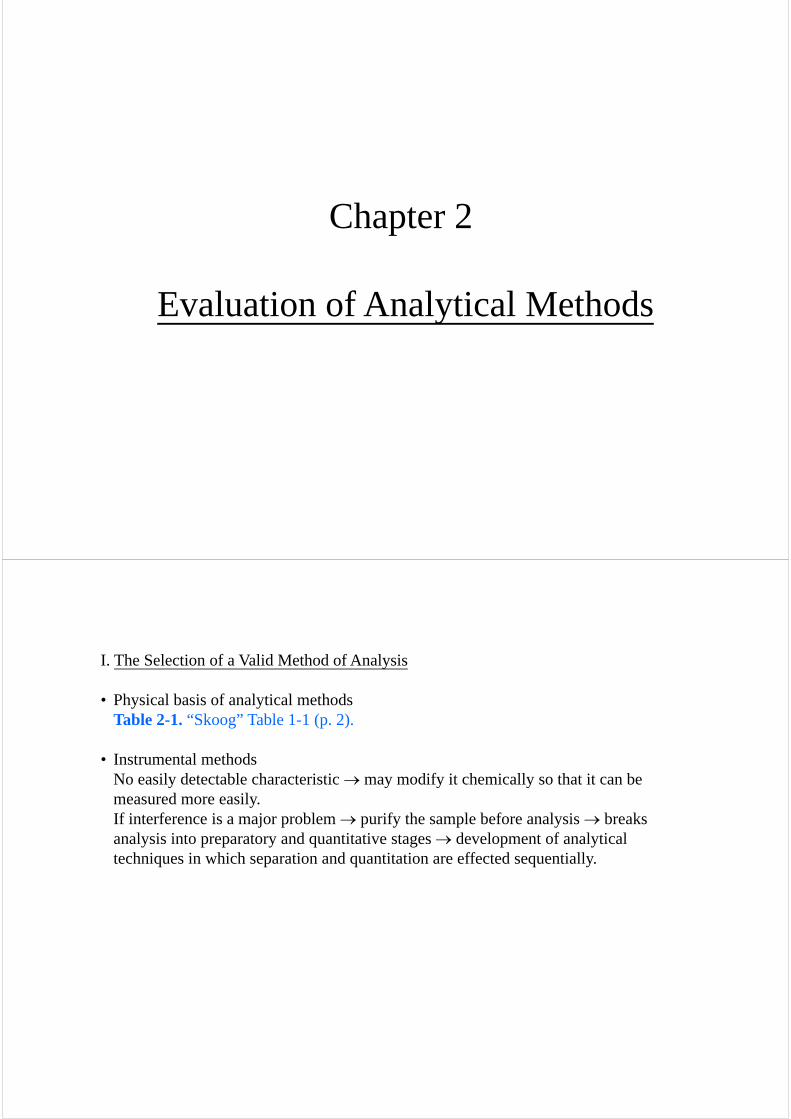
Table 2-2. “Skoog” Table 1-5 (p. 6).Table 2-3. “Holme” Table 1.4 (p. 7).

• Systematic errorSystematic errors cause inaccurate (incorrect) results and are referred to in terms of accuracy.

Bias = - 0

where is the population mean for the concentration of an analyte in a sample that has a true concentration of 0.

Determining bias involves analyzing one or more standard reference materials whose analyte concentration is known.Systematic errors have three sources: instrumental, personal, and method.

Standard error of the mean:

SEM = s/n1/2

TABLE 2-2. D.A. Skoog & J.J. Leary, Principles of Instrumental Analysis, 4th Ed., 1992.

TABLE 2-3. D.J. Holme & H. Peck, Analytical Biochemistry, 2nd Ed., Longman, 1993.

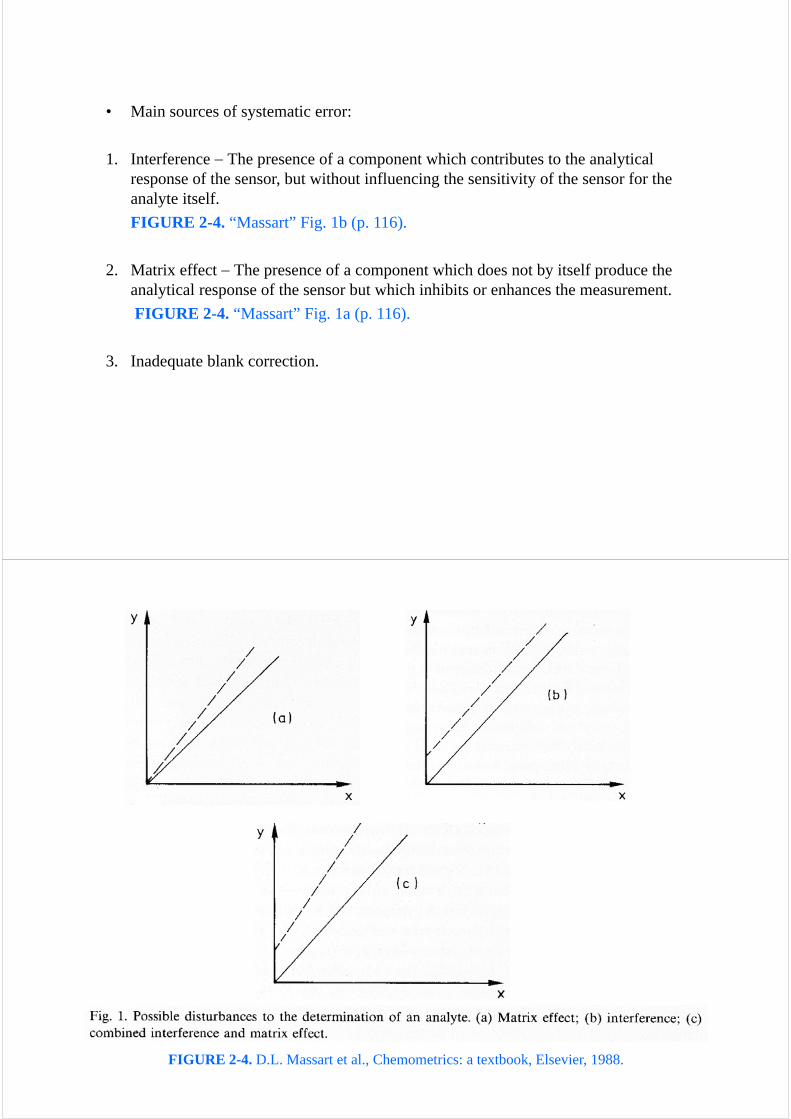
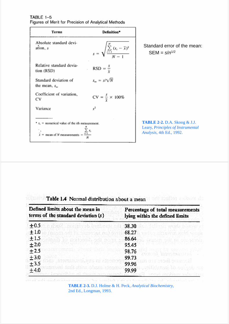
• Main sources of systematic error:

1. Interference The presence of a component which contributes to the analytical response of the sensor, but without influencing the sensitivity of the sensor for the analyte itself.

FIGURE 2-4. “Massart” Fig. 1b (p. 116).

2. Matrix effect The presence of a component which does not by itself produce the analytical response of the sensor but which inhibits or enhances the measurement.

FIGURE 2-4. “Massart” Fig. 1a (p. 116).

3. Inadequate blank correction.

FIGURE 2-4. D.L. Massart et al., Chemometrics: a textbook, Elsevier, 1988.

2. Signal-to-Noise Ratio

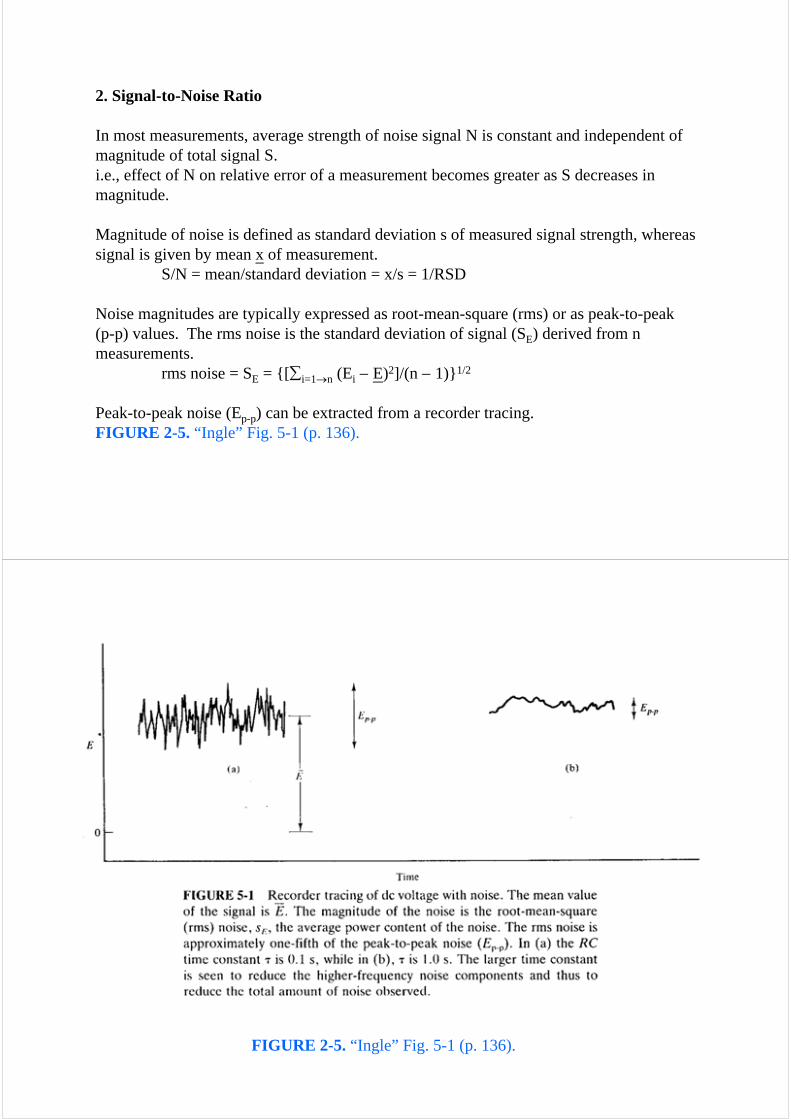
In most measurements, average strength of noise signal N is constant and independent of magnitude of total signal S.i.e., effect of N on relative error of a measurement becomes greater as S decreases in magnitude.

Magnitude of noise is defined as standard deviation s of measured signal strength, whereas signal is given by mean x of measurement.

S/N = mean/standard deviation = x/s = 1/RSD

Noise magnitudes are typically expressed as root-mean-square (rms) or as peak-to-peak (p-p) values. The rms noise is the standard deviation of signal (SE) derived from n measurements.

rms noise = SE = {[i=1n (Ei E)2]/(n 1)}1/2

Peak-to-peak noise (Ep-p) can be extracted from a recorder tracing.FIGURE 2-5. “Ingle” Fig. 5-1 (p. 136).

FIGURE 2-5. “Ingle” Fig. 5-1 (p. 136).

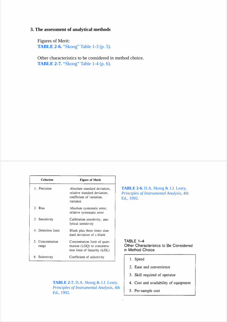
3. The assessment of analytical methods

Figures of Merit:TABLE 2-6. “Skoog” Table 1-3 (p. 5).

Other characteristics to be considered in method choice.TABLE 2-7. “Skoog” Table 1-4 (p. 6).

TABLE 2-6. D.A. Skoog & J.J. Leary, Principles of Instrumental Analysis, 4th Ed., 1992.

TABLE 2-7. D.A. Skoog & J.J. Leary, Principles of Instrumental Analysis, 4th Ed., 1992.

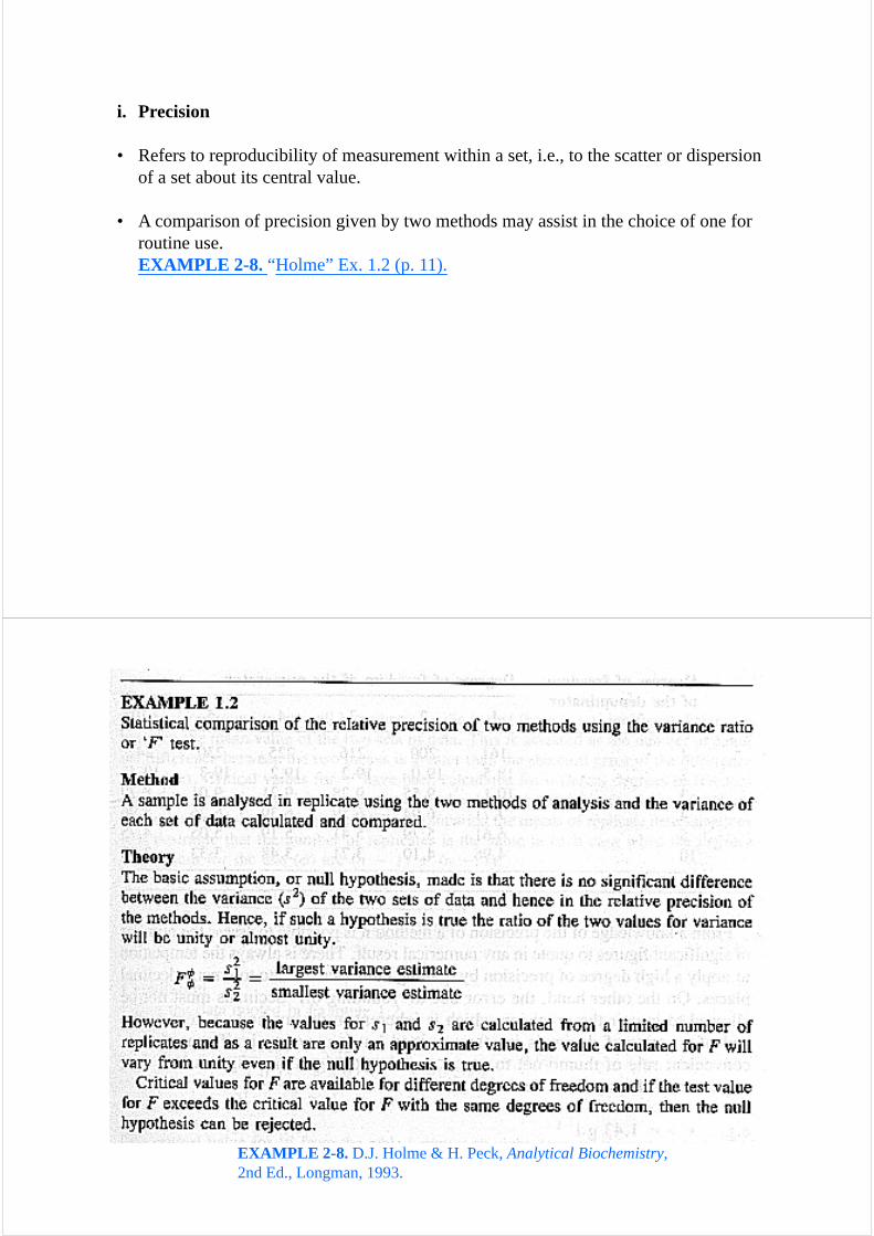
i. Precision

• Refers to reproducibility of measurement within a set, i.e., to the scatter or dispersion of a set about its central value.

• A comparison of precision given by two methods may assist in the choice of one for routine use.EXAMPLE 2-8. “Holme” Ex. 1.2 (p. 11).

EXAMPLE 2-8. D.J. Holme & H. Peck, Analytical Biochemistry, 2nd Ed., Longman, 1993.

EXAMPLE 2-8 (Cont.). D.J. Holme & H. Peck, Analytical Biochemistry, 2nd Ed., Longman, 1993.

EXAMPLE 2-8 (Cont.). D.J. Holme & H. Peck, Analytical Biochemistry, 2nd Ed., Longman, 1993.

ii. Accuracy

• Defined as closeness of the mean of replicate analyses to the true value of the sample.

• Assess accuracy by comparing the means of replicate analyses by two methods using the “t” test.EXAMPLE 2-9. “Holme” Ex. 1.3 (p. 13).

• Paired t-testEXAMPLE 2-10. “Miller” Sec. 3.4 (p. 58).

EXAMPLE 2-9. D.J. Holme & H. Peck, Analytical Biochemistry, 2nd Ed., Longman, 1993.

Alternatively, assuming population standard deviations are equal,

Pooled s2 = {(n11)s12+(n21)s2

2}/(n1+n21)

t = (x1 x2)/{s(1/n1+1/n2)1/2}

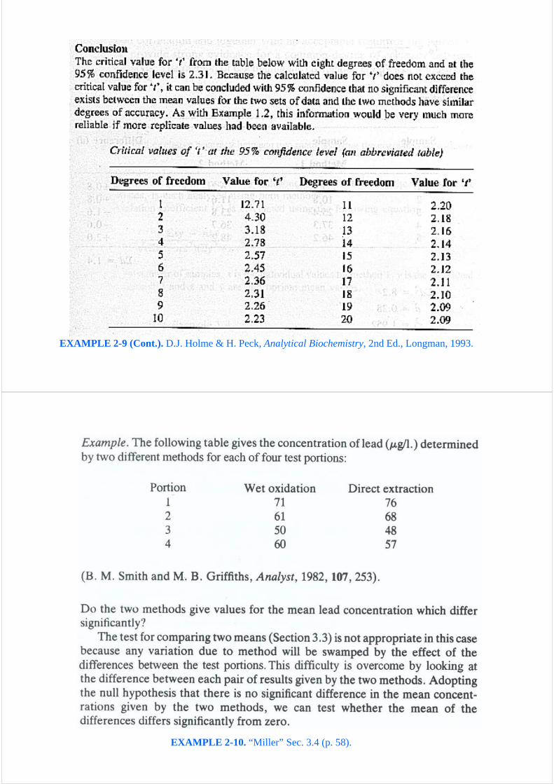
EXAMPLE 2-9 (Cont.). D.J. Holme & H. Peck, Analytical Biochemistry, 2nd Ed., Longman, 1993.

EXAMPLE 2-10. “Miller” Sec. 3.4 (p. 58).

EXAMPLE 2-10 (Cont.). “Miller” Sec. 3.4 (p. 58).

iii. Sensitivity

Two factors limit sensitivity: the slope of the calibration curve, and the reproducibility or precision of the measuring device.Most calibration curves are linear:

y = mx + ybl or sensitivity, S = dy/dxwhere y = measured signal

x = concentration of the analyteybl = instrument signal for a blankm = slope of the straight line

FIGURE 2-11. “Massart” Fig. 3 (p. 110).The slope of the calibration graph is a conventional way of expressing sensitivity and is particularly useful when comparing two methods.

a) Calibration sensitivity = m

b) Analytical sensitivity, = m/ss

where ss = standard deviation of the signalsAdvantages:

1. Relatively insensitive to amplification factors,2. Independent of the measurement units for S.

Disadvantage:Often concentration dependent, because ss often varies with concentration.

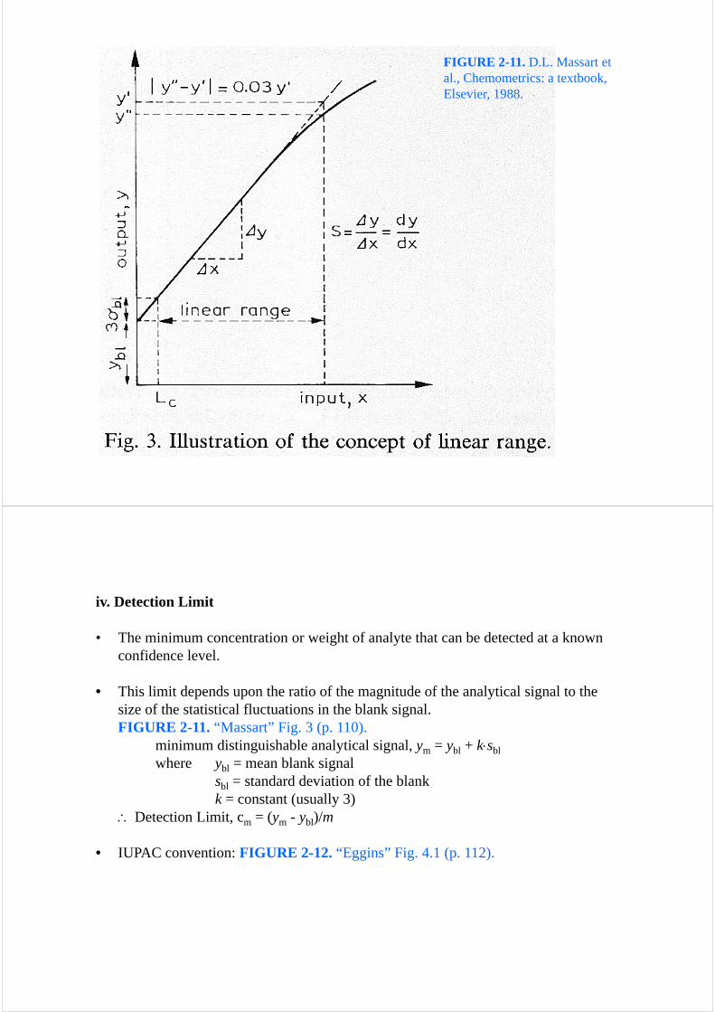
FIGURE 2-11. D.L. Massart et al., Chemometrics: a textbook, Elsevier, 1988.

iv. Detection Limit

• The minimum concentration or weight of analyte that can be detected at a known confidence level.

• This limit depends upon the ratio of the magnitude of the analytical signal to the size of the statistical fluctuations in the blank signal.FIGURE 2-11. “Massart” Fig. 3 (p. 110).

minimum distinguishable analytical signal, ym = ybl + ksbl

where ybl = mean blank signalsbl = standard deviation of the blankk = constant (usually 3)

Detection Limit, cm = (ym - ybl)/m

• IUPAC convention: FIGURE 2-12. “Eggins” Fig. 4.1 (p. 112).

FIGURE 2-12. B.R. Eggins, Chemical Sensors and Biosensors, Wiley, 2002.

v. Applicable Concentration Range (Linear Dynamic Range)• From the lowest concentration at which quantitative measurements can be made (limit

of quantitation, LOQ) to the concentration at which the calibration curve departs from linearity (limit of linearity, LOL).FIGURE 2-11. “Massart” Fig. 3 (p. 110).

• LOQ is generally taken as being equal to ten times the standard deviation when the analyte concentration is zero (i.e., 10sbl).

• An analytical method should have a range of at least two orders of magnitude.

vi. Selectivity• An interfering substance is defined as one that causes a predetermined systematic

error in the analytical results.• Selectivity coefficient: the degree to which it is free from interference by other

species contained in the sample matrix.e.g., A sample containing an analyte A and a potential interfering species B.

y = mACA + mBCB + yblDefine the selectivity coefficient for B with respect to A as

kB,A = mB/mASubstituting,

y = mA(CA + kB,ACB) + ybl

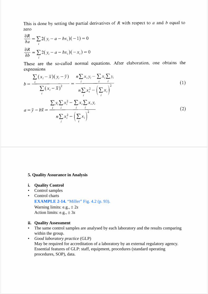
4. CalibrationCalibration function, y = g(x)For most analytical techniques, y = a + bx

i/. The method of least squaresRelationship between each observation pair can be represented as

yi = + xi + ei

FIGURE 2-12. “Massart” Fig. 1 (p. 76).

FIGURE 2-12. D.L. Massart et al., Chemometrics: a textbook, Elsevier, 1988.

5. Quality Assurance in Analysis

i. Quality Control• Control samples• Control charts

EXAMPLE 2-14. “Miller” Fig. 4.2 (p. 93).Warning limits: e.g., 2sAction limits: e.g., 3s

ii. Quality Assessment• The same control samples are analysed by each laboratory and the results comparing

within the group.• Good laboratory practice (GLP)

May be required for accreditation of a laboratory by an external regulatory agency.Essential features of GLP: staff, equipment, procedures (standard operating procedures, SOP), data.

EXAMPLE 2-14. J. C. Miller & J. N. Miller, Statistics for Analytical Chemistry, 3rd Ed., Ellis Horwood and Prentice Hall, 1993.