Chapter 18 Technology First understand the technology constraint of a firm. Later we will talk about constraints imposed by consumers and firm’s competitors.

• Chapter 18 Technology• First understand the technology constraint

of a firm. Later we will talk about constraints imposed by consumers and firm’s competitors (the demand curve faced by the firm, the market structure)

• Inputs: labor and capital• Inputs and outputs measured in flow units,

i.e., how many units of labor per week, how many units of output per week, etc.

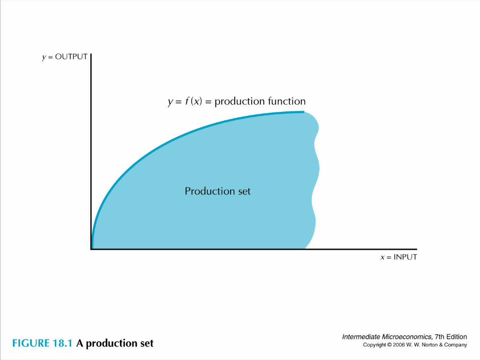
• Consider the case of one input (x) and one output (y). To describe the tech constraint of a firm, list all the technologically feasible ways to produce a given amount of outputs.

• The set of all combinations of inputs and outputs that comprise a technologically feasible way to produce is called a production set.

• A production function measures the maximum possible output that you can get from a given amount of input.

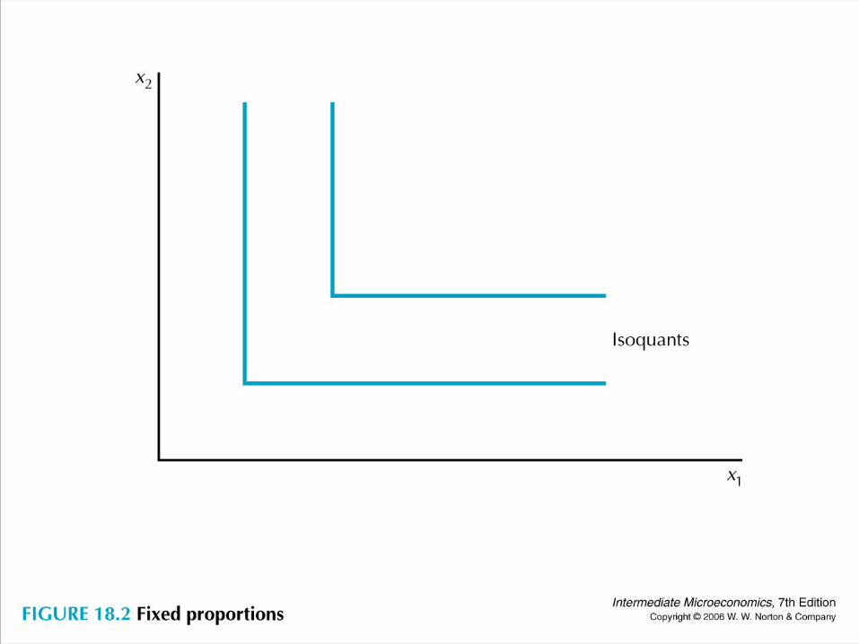
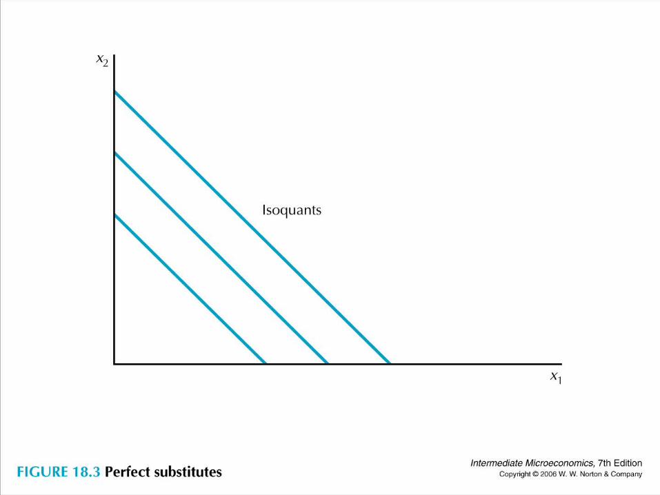
• Isoquant is another way to express the production function. It is a set of all possible combinations of inputs that are just sufficient to produce a given amount of output. Isoquant looks very much like indifference curve, but you cannot label it arbitrarily, neither can you do any monotonic transformation of the label.

• Some useful examples of production function. Two inputs, x1 and x2.

• Fixed proportion (perfect complement): f(x1,x2)=min{x1,x2}

• Perfect substitutes: f(x1,x2)=x1+x2

• Cobb-Douglas f(x1,x2)=A(x1)a(x2)b, cannot normalize to a+b=1 arbitrarily

• Some often-used assumptions on the production function

• Monotonicity: if you increase the amount of at least one input, you produce at least as much output as before

• Monotonicity holds because of free disposal, that is, can free dispose of any extra inputs

• Convexity: if y=f(x1,x2)=f(z1,z2), then f(tx1+(1-t)z1,tx2+(1-t)z2)y for any t[0,1]

• Some terms often used to describe the production function

• Marginal product: operate at (x1,x2), increase a bit of x1 and hold x2, how much more y can we get per additional unit of x1?

• Marginal product of factor 1: MP1(x1,x2)=∆y/∆x1=(f(x1+ ∆x1,x2)-f(x1,x2))/∆x1 (it is a rate, just like MU)

• Marginal rate of technical substitution factor 1 for factor 2: operate at (x1,x2), increase a bit of x1 and hold y, how much less x2 can you use? Measures the trade-off between two inputs in production

• MRTS1,2(x1,x2)=∆x2/∆x1=?

• ∆y=MP1(x1,x2)∆x1+MP2(x1,x2)∆x2=0

• MRTS1,2(x1,x2)=∆x2/∆x1=-MP1(x1,x2)/MP2(x1,x2) (it is a slope, just like MRS)

• Law of diminishing marginal product: holding all other inputs fixed, if we increase one input, the marginal product of that input becomes smaller and smaller (diminishing MU)

• Diminishing MRTS: the slope of an isoquant decreases in absolute value as we increase x1 (diminishing MRS)

• Short run: at least one factor of production is fixed

• Long run: all factors of production can be varied

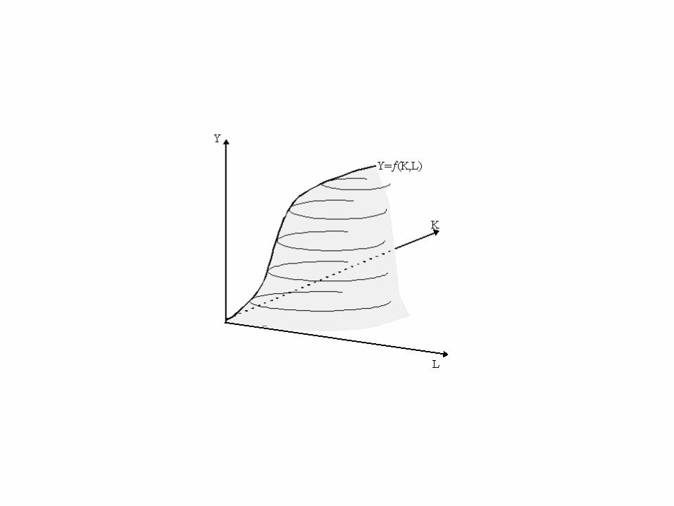
• Can also plot the short run production function y=f(x1,k)

• Returns to scale: if we use twice as much of each input, how much output will we get?

• constant returns to scale (CRS): for all t>0, f(tx1,tx2)=tf(x1,x2)

• Idea is if we double the inputs, we can just set two plants and so we can double the outputs

• Increasing returns to scale (IRS): for all t>1, f(tx1,tx2)>tf(x1,x2)

• Decreasing returns to scale (DRS): for all t>1, f(tx1,tx2)<tf(x1,x2)

• MP, MRTS, returns to scale