FOR SCIENTISTS AND ENGINEERS A STRATEGIC APPROACH 4/E PHYSICS RANDALL D. KNIGHT Chapter 17 Lecture © 2017 Pearson Education, Inc.

Welcome message from author
This document is posted to help you gain knowledge. Please leave a comment to let me know what you think about it! Share it to your friends and learn new things together.
Transcript
FOR SCIENTISTS AND ENGINEERS A STRATEGIC APPROACH 4/E PHYSICS
RANDALL D. KNIGHT
Chapter 17 Lecture
© 2017 Pearson Education, Inc.

© 2017 Pearson Education, Inc.
Chapter 17 Superposition
IN THIS CHAPTER, you will understand and use the ideas of superposition.
Slide 17-2

© 2017 Pearson Education, Inc.
Chapter 17 Preview
Slide 17-3
© 2017 Pearson Education, Inc.
Chapter 17 Preview
Slide 17-4
© 2017 Pearson Education, Inc.
Chapter 17 Preview
Slide 17-5
© 2017 Pearson Education, Inc.
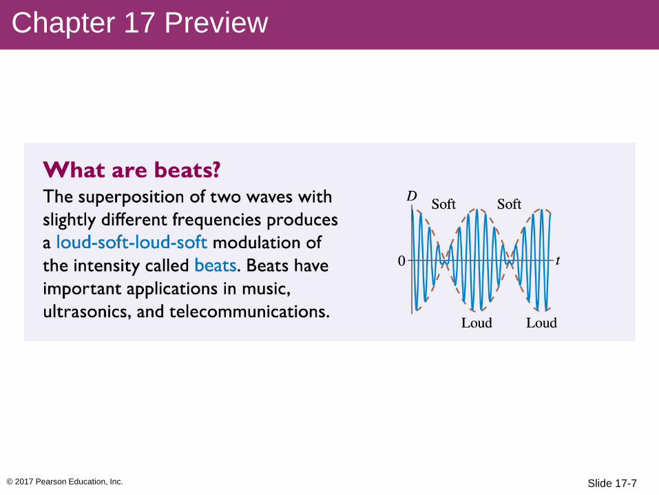
Chapter 17 Preview
Slide 17-6
© 2017 Pearson Education, Inc.
Chapter 17 Preview
Slide 17-7

© 2017 Pearson Education, Inc.
Chapter 17 Preview
Slide 17-8

© 2017 Pearson Education, Inc.
Chapter 17 Content, Examples, and QuickCheck Questions
Slide 17-9
© 2017 Pearson Education, Inc.
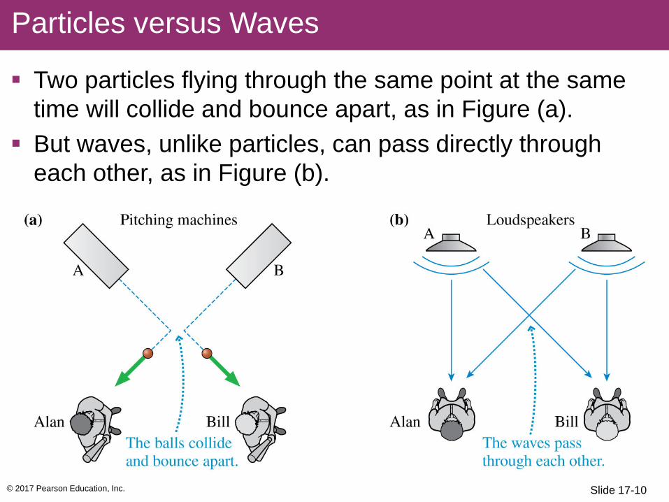
Two particles flying through the same point at the same time will collide and bounce apart, as in Figure (a).
But waves, unlike particles, can pass directly through each other, as in Figure (b).
Particles versus Waves
Slide 17-10
© 2017 Pearson Education, Inc.
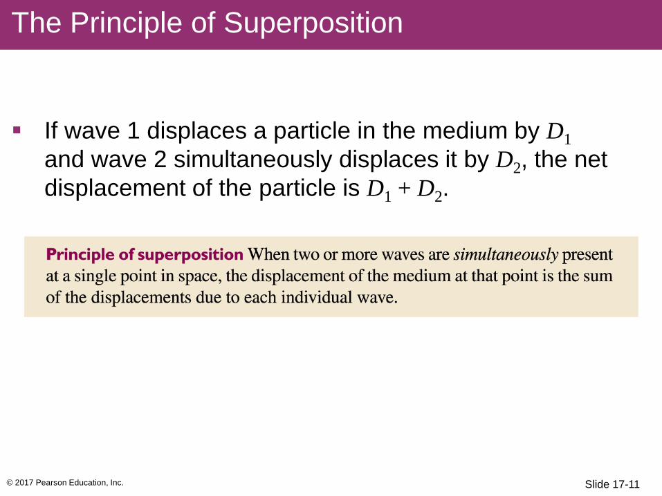
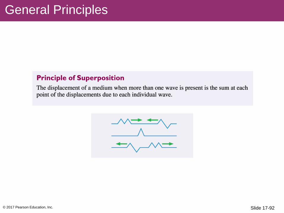
If wave 1 displaces a particle in the medium by D1 and wave 2 simultaneously displaces it by D2, the net displacement of the particle is D1 + D2.
The Principle of Superposition
Slide 17-11

© 2017 Pearson Education, Inc.
The figure shows the superposition of two waves on a string as they pass through each other.
The principle of superposition comes into play wherever the waves overlap.
The solid line is the sum at each point of the two displacements at that point.
The Principle of Superposition
Slide 17-12
© 2017 Pearson Education, Inc.
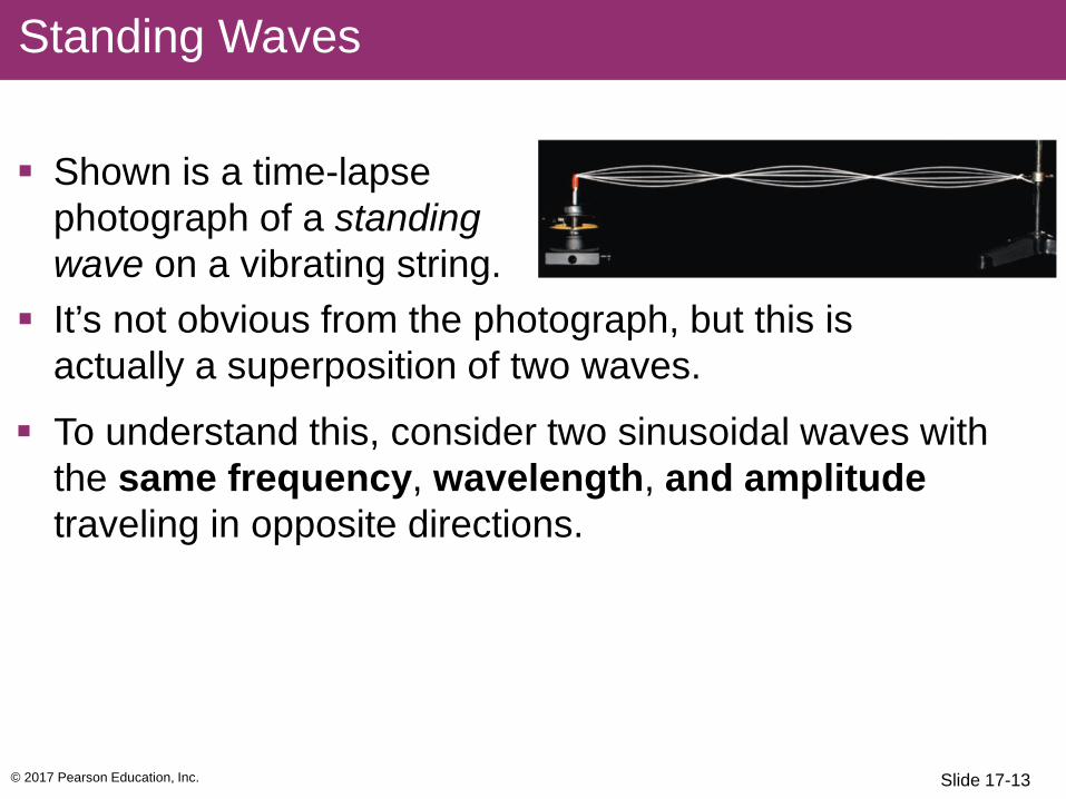
Shown is a time-lapse photograph of a standing wave on a vibrating string.
It’s not obvious from the photograph, but this is actually a superposition of two waves.
To understand this, consider two sinusoidal waves with the same frequency, wavelength, and amplitude traveling in opposite directions.
Standing Waves
Slide 17-13

© 2017 Pearson Education, Inc.
Standing Waves
Antinode Node Slide 17-14
© 2017 Pearson Education, Inc.
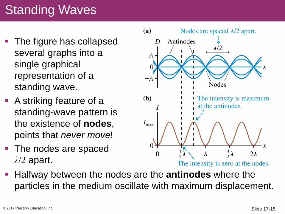
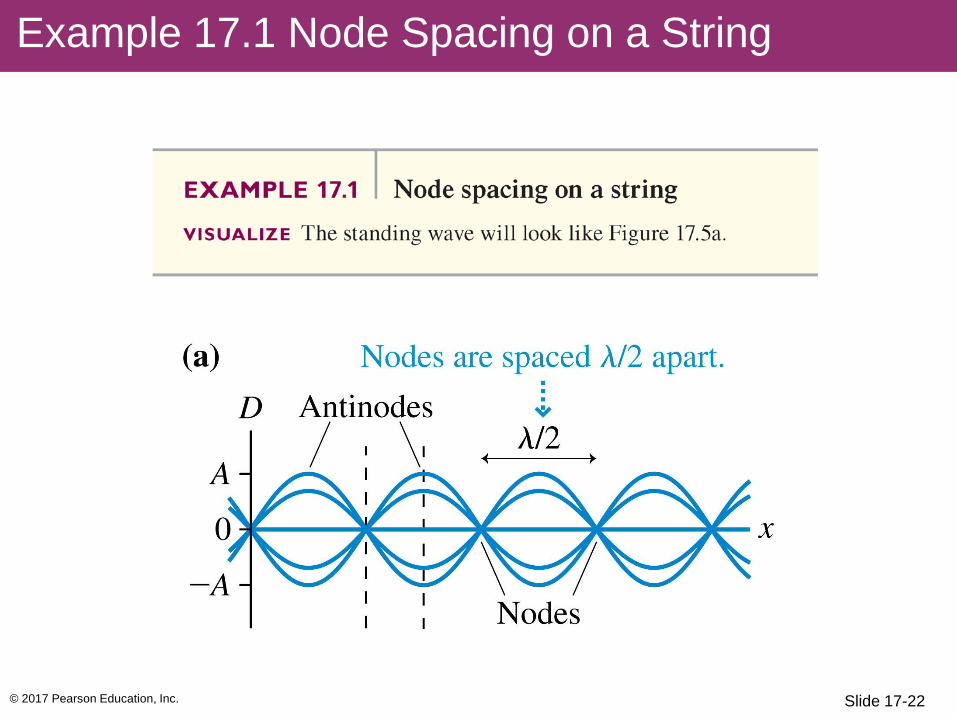
The figure has collapsed several graphs into a single graphical representation of a standing wave.
A striking feature of a standing-wave pattern is the existence of nodes, points that never move!
The nodes are spaced λ/2 apart.
Halfway between the nodes are the antinodes where the particles in the medium oscillate with maximum displacement.
Standing Waves
Slide 17-15

© 2017 Pearson Education, Inc.
In Chapter 16 you learned that the intensity of a wave is proportional to the square of the amplitude:
Intensity is maximum at points of constructive interference and zero at points of destructive interference.
Standing Waves
Slide 17-16

© 2017 Pearson Education, Inc.
This photograph shows the Tacoma Narrows suspension bridge just before it collapsed. Aerodynamic forces
caused the amplitude of a particular standing wave of the bridge to increase dramatically.
The red line shows the original line of the deck of the bridge.
Standing Waves
Slide 17-17

© 2017 Pearson Education, Inc.
A sinusoidal wave traveling to the right along the x-axis with angular frequency ω = 2πf, wave number k = 2π/λ and amplitude a is
An equivalent wave traveling to the left is
We previously used the symbol A for the wave amplitude, but here we will use a lowercase a to represent the amplitude of each individual wave and reserve A for the amplitude of the net wave.
The Mathematics of Standing Waves
Slide 17-18

© 2017 Pearson Education, Inc.
According to the principle of superposition, the net displacement of the medium when both waves are present is the sum of DR and DL:
We can simplify this by using a trigonometric identity, and arrive at
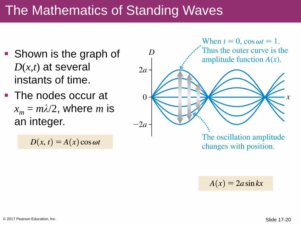
Where the amplitude function A(x) is defined as
The amplitude reaches a maximum value of Amax = 2a at points where sin kx = 1.
The Mathematics of Standing Waves
Slide 17-19
© 2017 Pearson Education, Inc.
Shown is the graph of D(x,t) at several instants of time.
The nodes occur at xm = mλ/2, where m is an integer.
The Mathematics of Standing Waves
Slide 17-20

© 2017 Pearson Education, Inc.
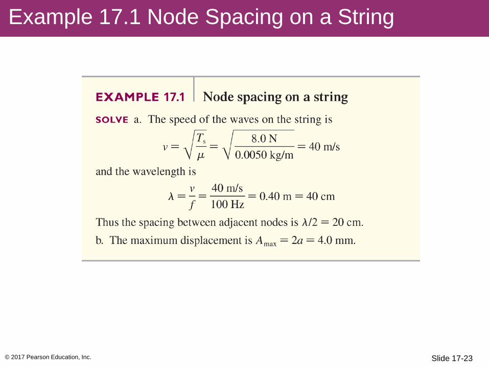
Example 17.1 Node Spacing on a String
Slide 17-21
© 2017 Pearson Education, Inc.
Example 17.1 Node Spacing on a String
Slide 17-22
© 2017 Pearson Education, Inc.
Example 17.1 Node Spacing on a String
Slide 17-23

© 2017 Pearson Education, Inc.
A string with a large linear density is connected to one with a smaller linear density. The tension is the same in both strings, so the wave
speed is slower on the left, faster on the right. When a wave
encounters such a discontinuity, some of the wave’s energy is transmitted forward and some is reflected.
Waves on a String with a Discontinuity
Slide 17-24
© 2017 Pearson Education, Inc.
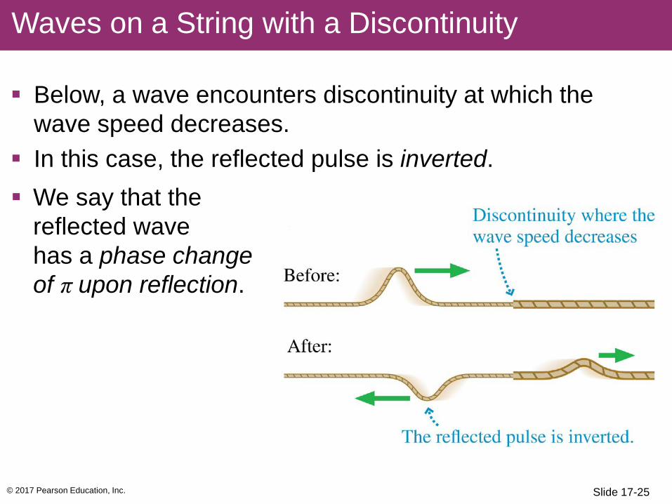
Below, a wave encounters discontinuity at which the wave speed decreases.
In this case, the reflected pulse is inverted. We say that the
reflected wave has a phase change of π upon reflection.
Waves on a String with a Discontinuity
Slide 17-25
© 2017 Pearson Education, Inc.
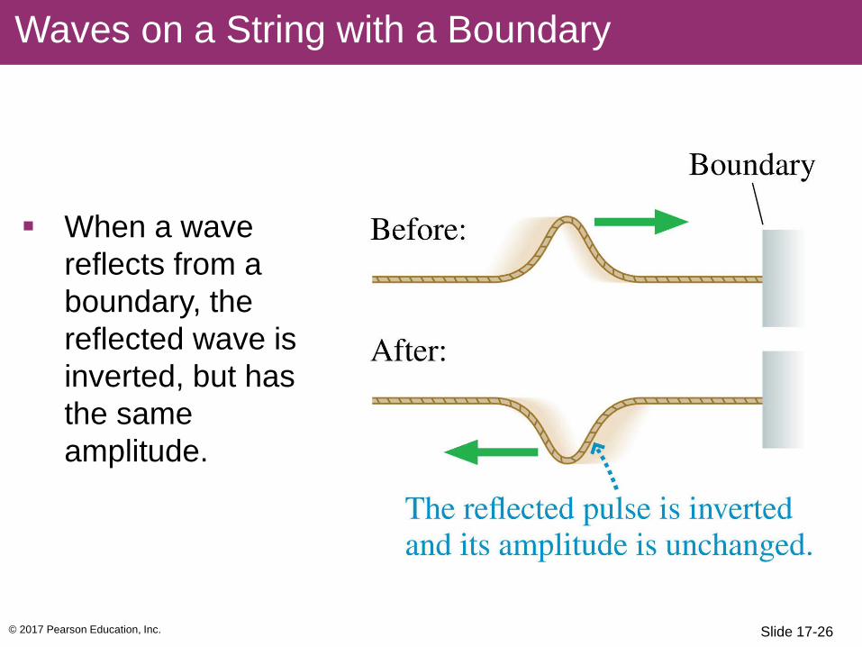
When a wave reflects from a boundary, the reflected wave is inverted, but has the same amplitude.
Waves on a String with a Boundary
Slide 17-26

© 2017 Pearson Education, Inc.
The figure shows a string of length L tied at x = 0 and x = L.
Reflections at the ends of the string cause waves of equal amplitude and wavelength to travel in opposite directions along the string.
These are the conditions that cause a standing wave!
Creating Standing Waves
Slide 17-27

© 2017 Pearson Education, Inc.
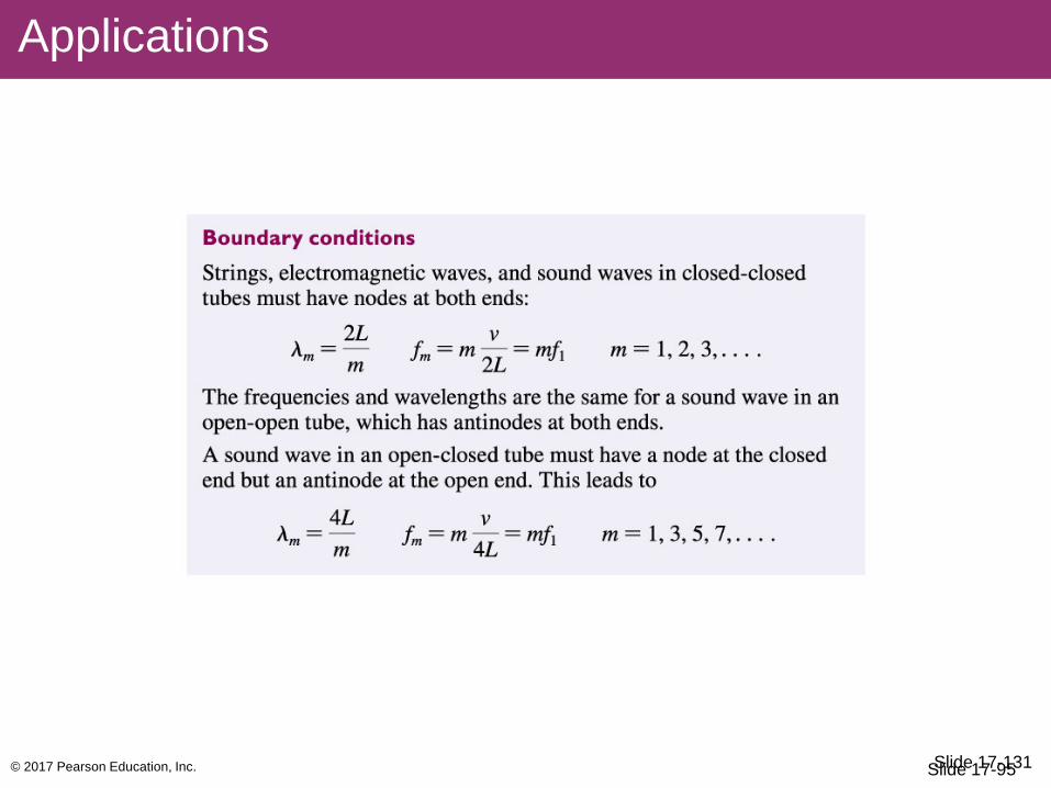
For a string of fixed length L, the boundary conditions can be satisfied only if the wavelength has one of the values:
Because λf = v for a sinusoidal wave, the oscillation frequency corresponding to wavelength λm is
The lowest allowed frequency is called the fundamental frequency: f1 = v/2L.
Standing Waves on a String
Slide 17-28
© 2017 Pearson Education, Inc.
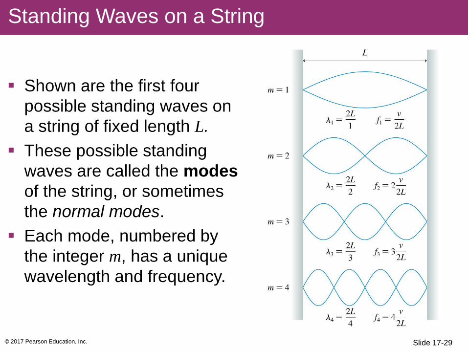
Shown are the first four possible standing waves on a string of fixed length L.
These possible standing waves are called the modes of the string, or sometimes the normal modes.
Each mode, numbered by the integer m, has a unique wavelength and frequency.
Standing Waves on a String
Slide 17-29

© 2017 Pearson Education, Inc.
m is the number of antinodes on the standing wave. The fundamental mode, with m = 1, has λ1 = 2L. The frequencies of the normal modes form a series:
f1, 2f1, 3f1, … The fundamental frequency f1 can be found as the
difference between the frequencies of any two adjacent modes: f1 = Δf = fm+1 – fm.
Below is a time-exposure photograph of the m = 3 standing wave on a string.
Standing Waves on a String
Slide 17-30
© 2017 Pearson Education, Inc.
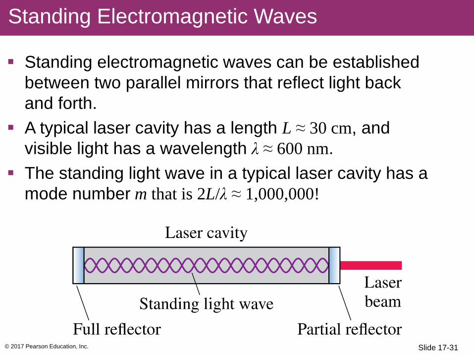
Standing electromagnetic waves can be established between two parallel mirrors that reflect light back and forth.
A typical laser cavity has a length L ≈ 30 cm, and visible light has a wavelength λ ≈ 600 nm.
The standing light wave in a typical laser cavity has a mode number m that is 2L/λ ≈ 1,000,000!
Standing Electromagnetic Waves
Slide 17-31

© 2017 Pearson Education, Inc.
Example 17.3 The Standing Light Wave Inside a Laser
Slide 17-32

© 2017 Pearson Education, Inc.
Example 17.3 The Standing Light Wave Inside a Laser
Slide 17-33

© 2017 Pearson Education, Inc.
A long, narrow column of air, such as the air in a tube or pipe, can support a longitudinal standing sound wave.
A closed end of a column of air must be a displacement node, thus the boundary conditions—nodes at the ends—are the same as for a standing wave on a string.
It is often useful to think of sound as a pressure wave rather than a displacement wave: The pressure oscillates around its equilibrium value.
The nodes and antinodes of the pressure wave are interchanged with those of the displacement wave.
Standing Sound Waves
Slide 17-34
© 2017 Pearson Education, Inc.
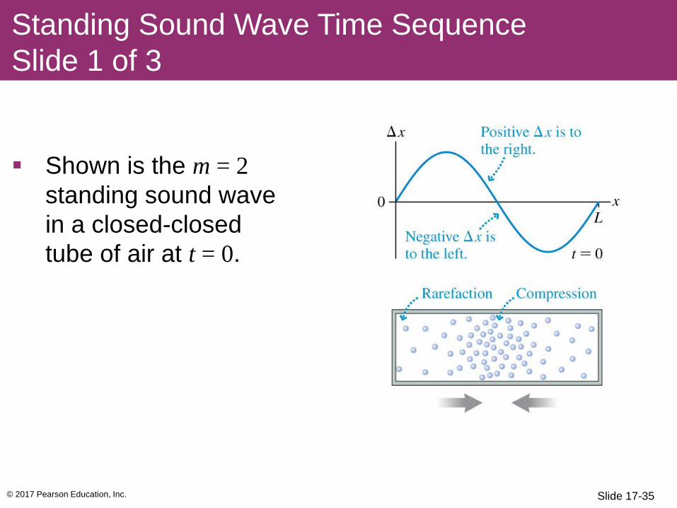
Shown is the m = 2 standing sound wave in a closed-closed tube of air at t = 0.
Standing Sound Wave Time Sequence Slide 1 of 3
Slide 17-35
© 2017 Pearson Education, Inc.
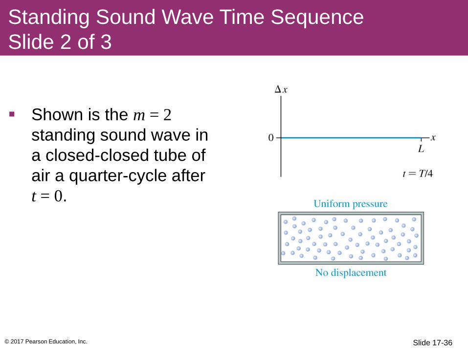
Shown is the m = 2 standing sound wave in a closed-closed tube of air a quarter-cycle after t = 0.
Standing Sound Wave Time Sequence Slide 2 of 3
Slide 17-36

© 2017 Pearson Education, Inc.
Shown is the m = 2 standing sound wave in a closed-closed tube of air a half-cycle after t = 0.
Standing Sound Wave Time Sequence Slide 3 of 3
Slide 17-37

© 2017 Pearson Education, Inc.
Shown are the displacement Δx and pressure graphs for the m = 2 mode of standing sound waves in a closed-closed tube.
The nodes and antinodes of the pressure wave are interchanged with those of the displacement wave.
Standing Sound Waves
Slide 17-38
© 2017 Pearson Education, Inc.
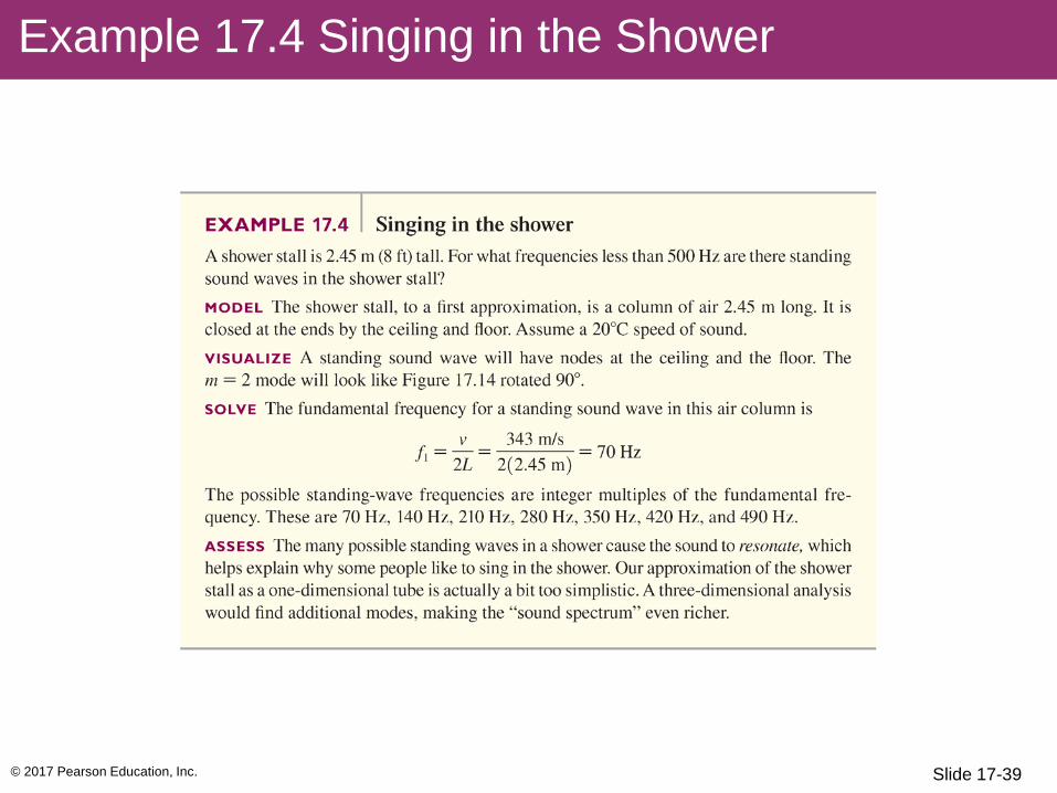
Example 17.4 Singing in the Shower
Slide 17-39
© 2017 Pearson Education, Inc.
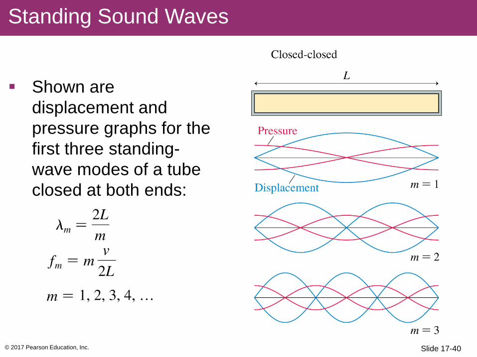
Shown are displacement and pressure graphs for the first three standing-wave modes of a tube closed at both ends:
Standing Sound Waves
Slide 17-40
© 2017 Pearson Education, Inc.
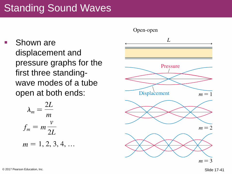
Shown are displacement and pressure graphs for the first three standing-wave modes of a tube open at both ends:
Standing Sound Waves
Slide 17-41
© 2017 Pearson Education, Inc.
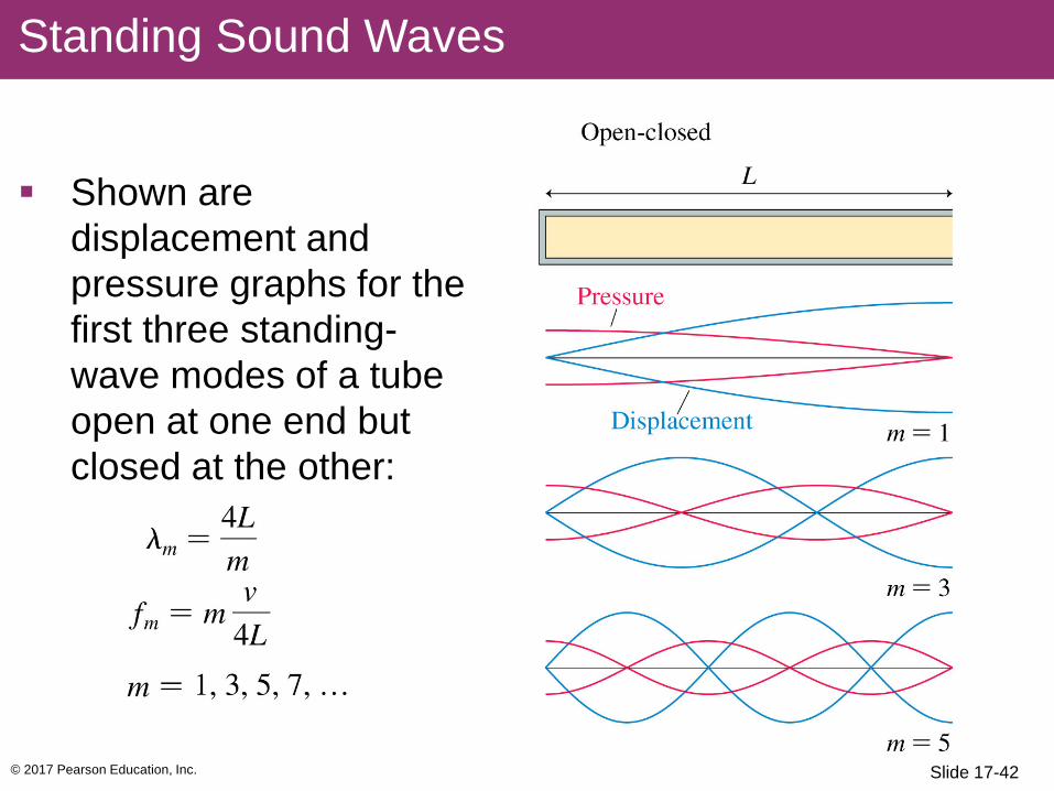
Shown are displacement and pressure graphs for the first three standing-wave modes of a tube open at one end but closed at the other:
Standing Sound Waves
Slide 17-42
© 2017 Pearson Education, Inc.
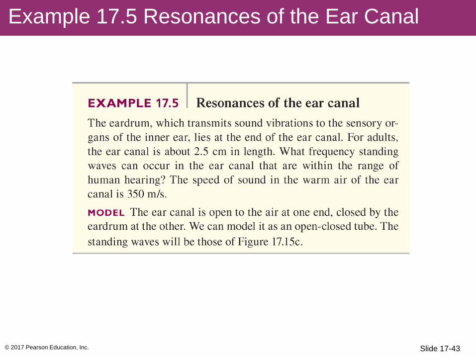
Example 17.5 Resonances of the Ear Canal
Slide 17-43
© 2017 Pearson Education, Inc.
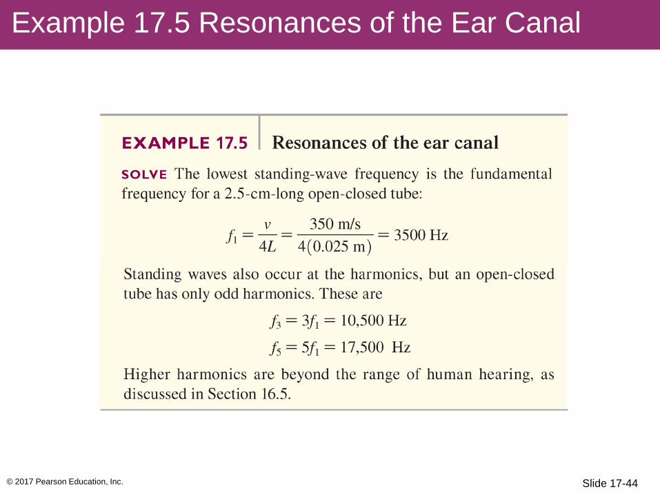
Example 17.5 Resonances of the Ear Canal
Slide 17-44
© 2017 Pearson Education, Inc.
Example 17.5 Resonances of the Ear Canal
Slide 17-45

© 2017 Pearson Education, Inc.
Instruments such as the harp, the piano, and the violin have strings fixed at the ends and tightened to create tension.
A disturbance generated on the string by plucking, striking, or bowing it creates a standing wave on the string.
The fundamental frequency is the musical note you hear when the string is sounded:
where Ts is the tension in the string and μ is its linear density.
Musical Instruments
Slide 17-46
© 2017 Pearson Education, Inc.
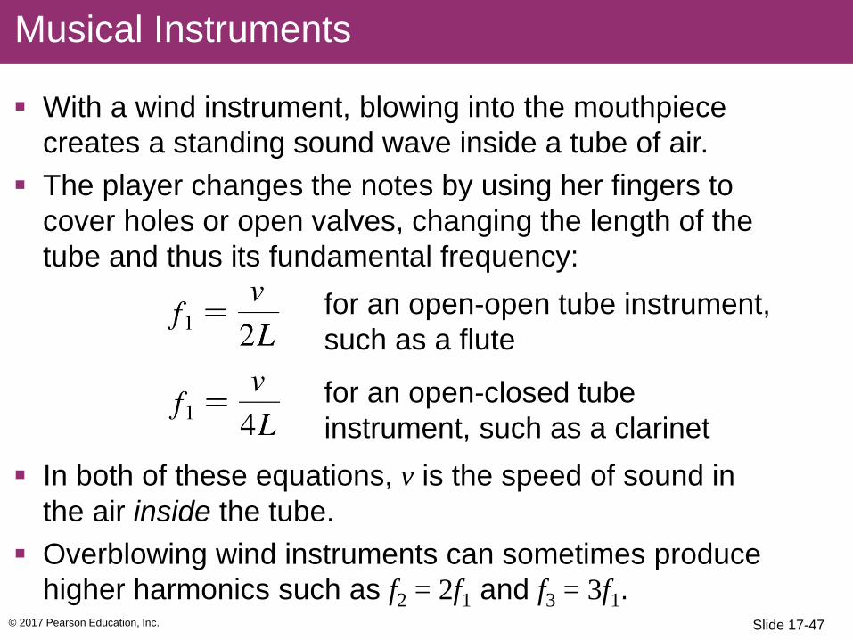
With a wind instrument, blowing into the mouthpiece creates a standing sound wave inside a tube of air.
The player changes the notes by using her fingers to cover holes or open valves, changing the length of the tube and thus its fundamental frequency:
In both of these equations, v is the speed of sound in the air inside the tube.
Overblowing wind instruments can sometimes produce higher harmonics such as f2 = 2f1 and f3 = 3f1.
for an open-open tube instrument, such as a flute
for an open-closed tube instrument, such as a clarinet
Musical Instruments
Slide 17-47
© 2017 Pearson Education, Inc.
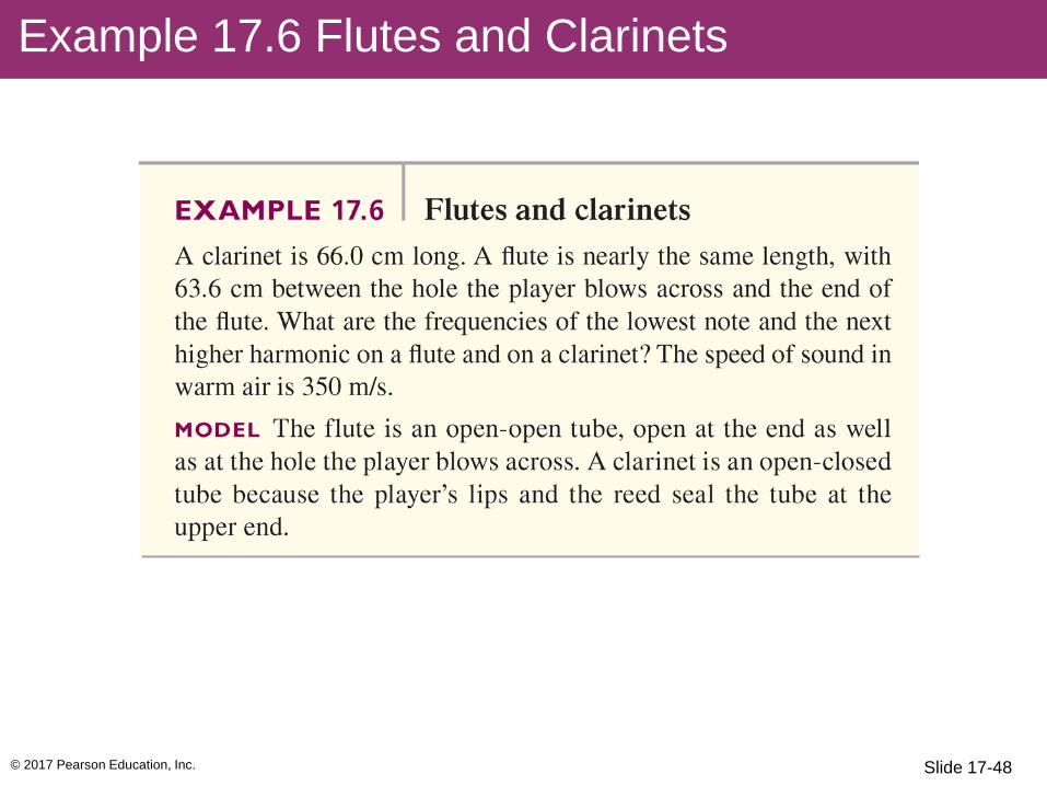
Example 17.6 Flutes and Clarinets
Slide 17-48

© 2017 Pearson Education, Inc.
Example 17.6 Flutes and Clarinets
Slide 17-49
© 2017 Pearson Education, Inc.
Example 17.6 Flutes and Clarinets
Slide 17-50
© 2017 Pearson Education, Inc.
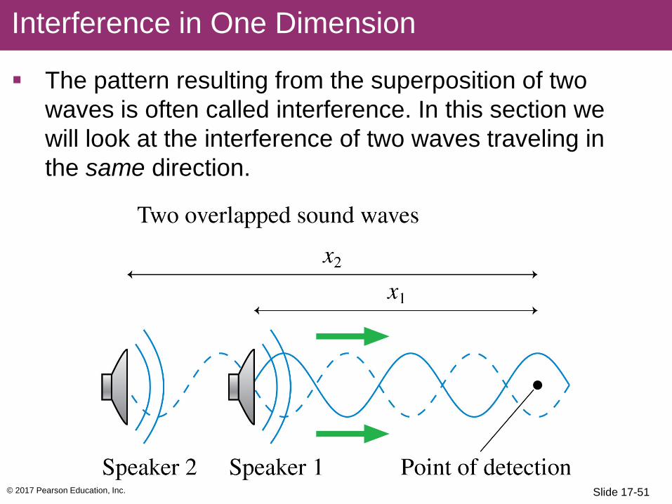
The pattern resulting from the superposition of two waves is often called interference. In this section we will look at the interference of two waves traveling in the same direction.
Interference in One Dimension
Slide 17-51
© 2017 Pearson Education, Inc.
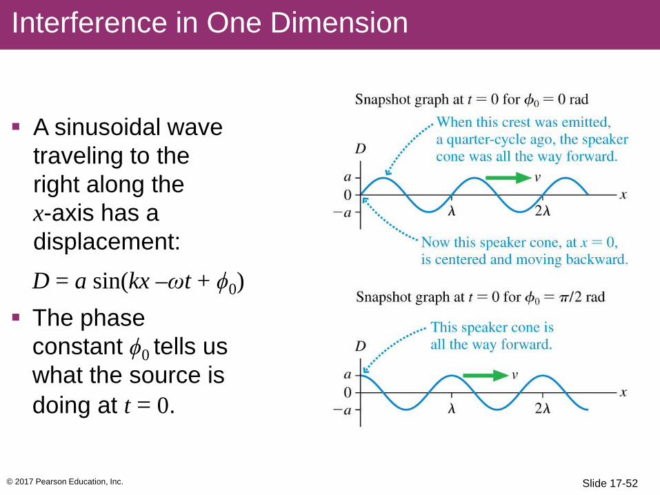
A sinusoidal wave traveling to the right along the x-axis has a displacement:
The phase constant ϕ0 tells us what the source is doing at t = 0.
Interference in One Dimension
D = a sin(kx –ωt + ϕ0)
Slide 17-52

© 2017 Pearson Education, Inc.
The two waves are in phase, meaning that
D1(x) = D2(x)
The resulting amplitude is A = 2a for maximum constructive interference.
Constructive Interference
D = D1 + D2
D1 = a sin(kx1 – ωt + ϕ10)
D2 = a sin(kx2 –ωt + ϕ20)
Slide 17-53

© 2017 Pearson Education, Inc.
Destructive Interference
The two waves are out of phase, meaning that
D1(x) = −D2(x)
The resulting amplitude is A = 0 for perfect destructive interference.
Slide 17-54
D = D1 + D2
D1 = a sin(kx1 – ωt + ϕ10)
D2 = a sin(kx2 –ωt + ϕ20)
© 2017 Pearson Education, Inc.
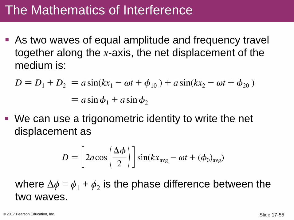
As two waves of equal amplitude and frequency travel together along the x-axis, the net displacement of the medium is:
We can use a trigonometric identity to write the net displacement as
where Δϕ = ϕ1 + ϕ2 is the phase difference between the two waves.
The Mathematics of Interference
Slide 17-55

© 2017 Pearson Education, Inc.
The amplitude has a maximum value A = 2a if cos(Δϕ/2) = ±1.
This is maximum constructive interference, when
where m is an integer. Similarly, the amplitude is zero if cos(Δϕ/2) = 0. This is perfect destructive interference, when:
The Mathematics of Interference
Slide 17-56

© 2017 Pearson Education, Inc.
Shown are two identical sources located one wavelength apart:
Δx = λ The two waves are
“in step” with Δϕ = 2π, so we have maximum constructive interference with A = 2a.
Interference in One Dimension
Slide 17-57
© 2017 Pearson Education, Inc.
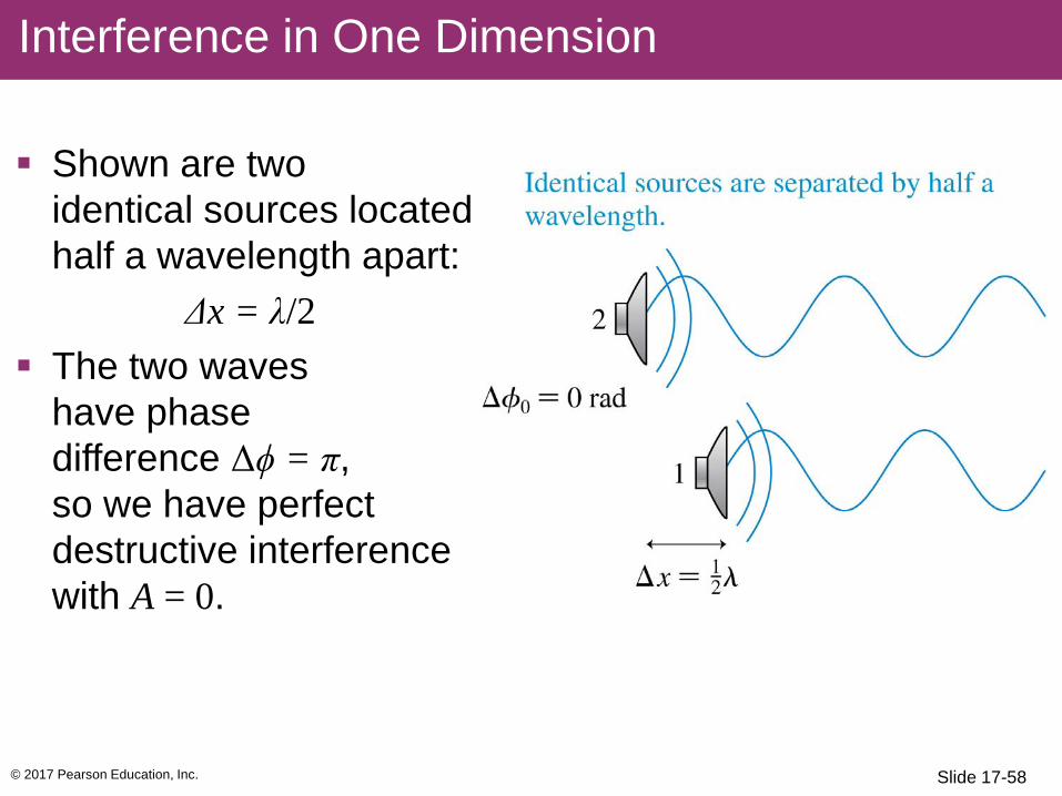
Shown are two identical sources located half a wavelength apart:
Δx = λ/2 The two waves
have phase difference Δϕ = π, so we have perfect destructive interference with A = 0.
Interference in One Dimension
Slide 17-58
© 2017 Pearson Education, Inc.
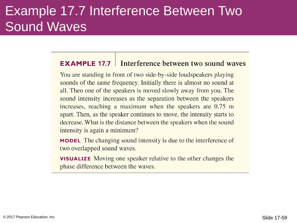
Example 17.7 Interference Between Two Sound Waves
Slide 17-59
© 2017 Pearson Education, Inc.
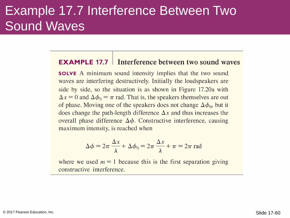
Example 17.7 Interference Between Two Sound Waves
Slide 17-60
© 2017 Pearson Education, Inc.
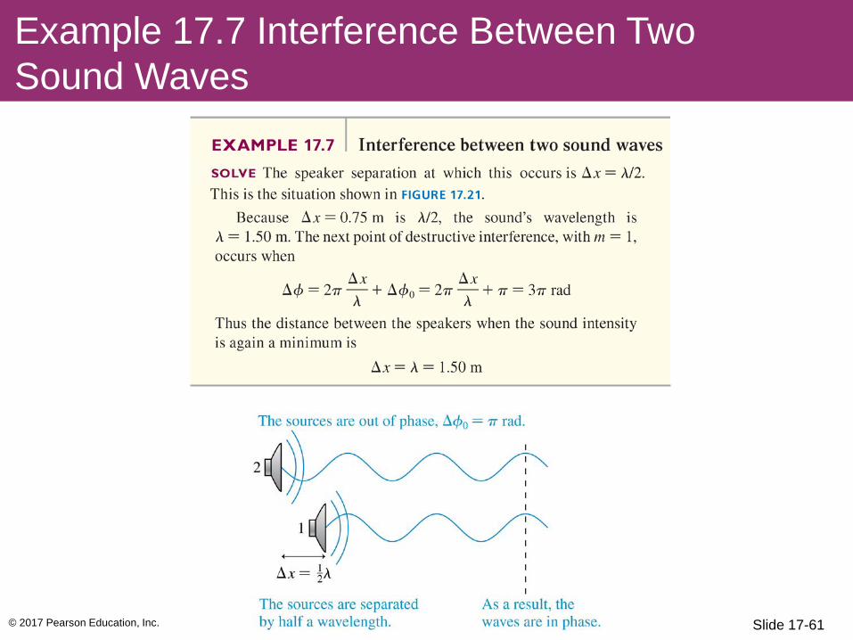
Example 17.7 Interference Between Two Sound Waves
Slide 17-61

© 2017 Pearson Education, Inc.
Example 17.7 Interference Between Two Sound Waves
Slide 17-62

© 2017 Pearson Education, Inc.
It is entirely possible, of course, that the two waves are neither exactly in phase nor exactly out of phase.
Shown are the calculated interference of two waves that differ in phase by 40º, 90º and 160º.
The Mathematics of Interference
Slide 17-63

© 2017 Pearson Education, Inc.
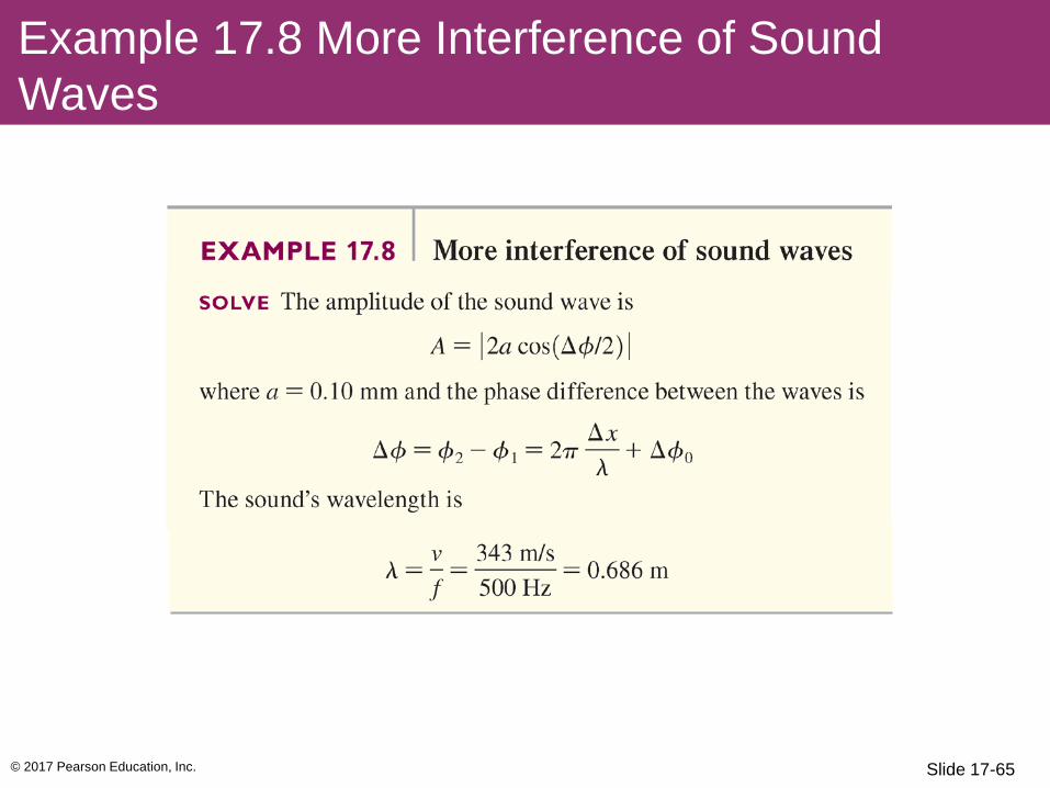
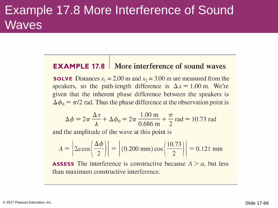
Example 17.8 More Interference of Sound Waves
Slide 17-64
© 2017 Pearson Education, Inc.
Example 17.8 More Interference of Sound Waves
Slide 17-65
© 2017 Pearson Education, Inc.
Example 17.8 More Interference of Sound Waves
Slide 17-66

© 2017 Pearson Education, Inc.
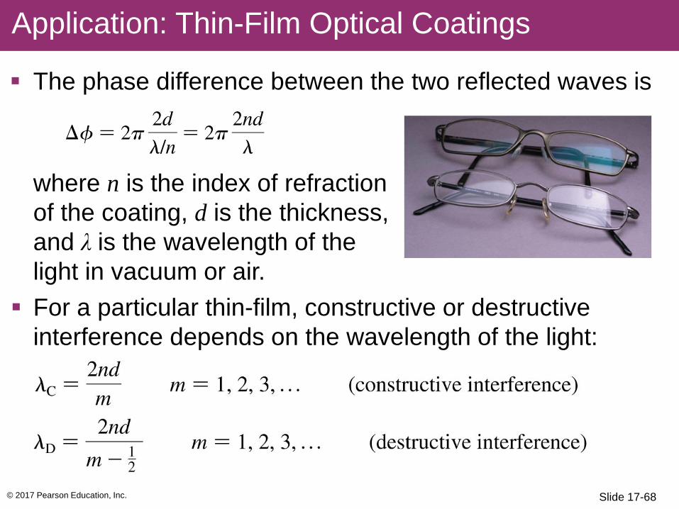
Thin transparent films, placed on glass surfaces, such as lenses, can control reflections from the glass.
Antireflection coatings on the lenses in cameras, microscopes, and other optical equipment are examples of thin-film coatings.
Application: Thin-Film Optical Coatings
Slide 17-67
© 2017 Pearson Education, Inc.
The phase difference between the two reflected waves is
where n is the index of refraction of the coating, d is the thickness, and λ is the wavelength of the light in vacuum or air.
For a particular thin-film, constructive or destructive interference depends on the wavelength of the light:
Application: Thin-Film Optical Coatings
Slide 17-68

© 2017 Pearson Education, Inc.
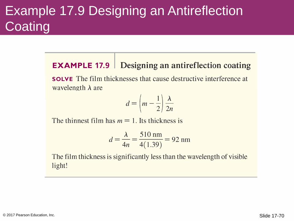
Example 17.9 Designing an Antireflection Coating
Slide 17-98 Slide 17-69
© 2017 Pearson Education, Inc.
Example 17.9 Designing an Antireflection Coating
Slide 17-70
© 2017 Pearson Education, Inc.
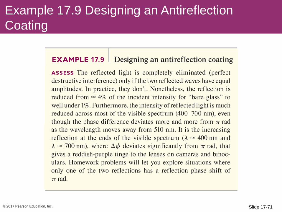
Example 17.9 Designing an Antireflection Coating
Slide 17-71
© 2017 Pearson Education, Inc.
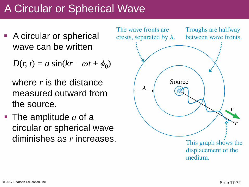
A circular or spherical wave can be written
where r is the distance measured outward from the source.
The amplitude a of a circular or spherical wave diminishes as r increases.
A Circular or Spherical Wave
D(r, t) = a sin(kr – ωt + ϕ0)
Slide 17-72

© 2017 Pearson Education, Inc.
Interference in Two and Three Dimensions
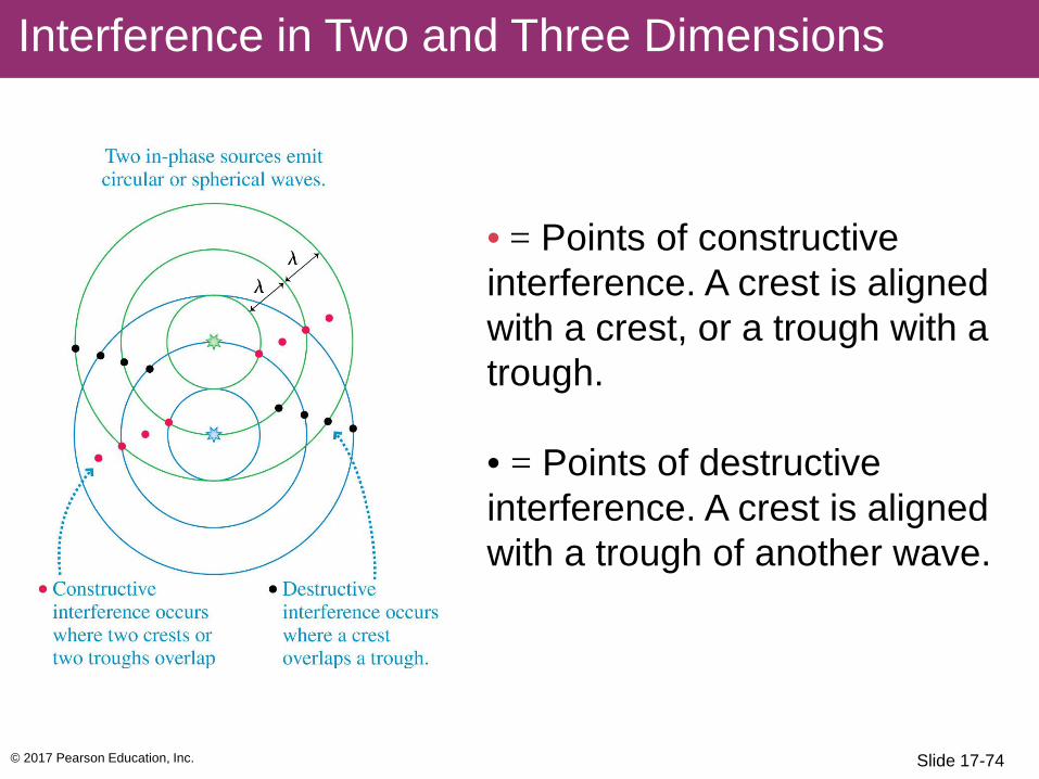
Two overlapping water waves create an interference pattern.
Slide 17-73
© 2017 Pearson Education, Inc.
• = Points of constructive interference. A crest is aligned with a crest, or a trough with a trough. • = Points of destructive interference. A crest is aligned with a trough of another wave.
Interference in Two and Three Dimensions
Slide 17-74
© 2017 Pearson Education, Inc.
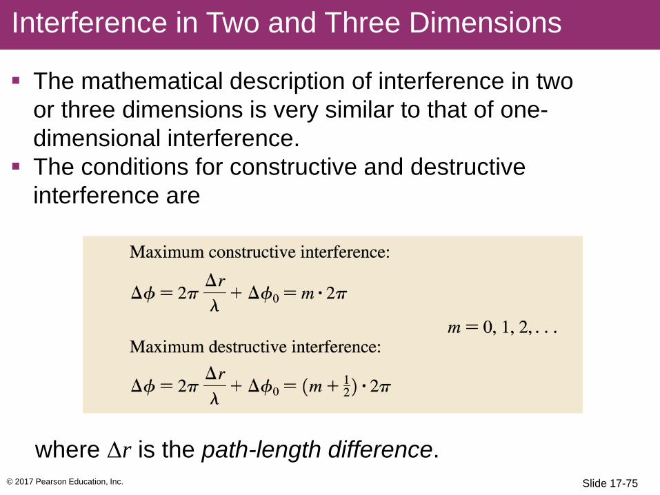
The mathematical description of interference in two or three dimensions is very similar to that of one-dimensional interference.
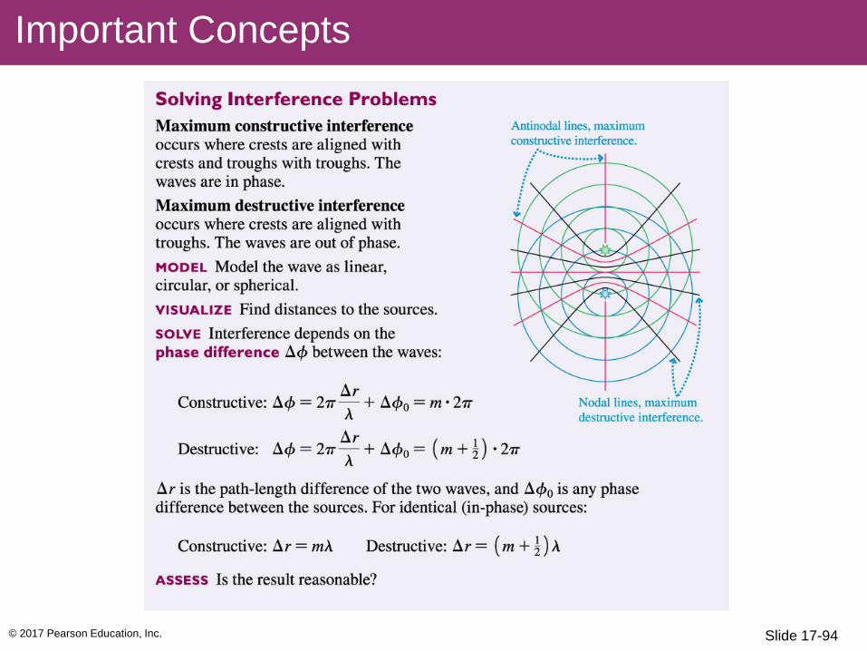
The conditions for constructive and destructive interference are
where Δr is the path-length difference.
Interference in Two and Three Dimensions
Slide 17-75

© 2017 Pearson Education, Inc.
The figure shows two identical sources that are in phase.
The path-length difference Δr determines whether the interference at a particular point is constructive or destructive.
Interference in Two and Three Dimensions
Slide 17-76

© 2017 Pearson Education, Inc.
Interference in Two and Three Dimensions
Slide 17-77

© 2017 Pearson Education, Inc.
Problem-Solving Strategy: Interference of Two Waves
Slide 17-78

© 2017 Pearson Education, Inc.
Problem-Solving Strategy: Interference of Two Waves
Slide 17-79
© 2017 Pearson Education, Inc.
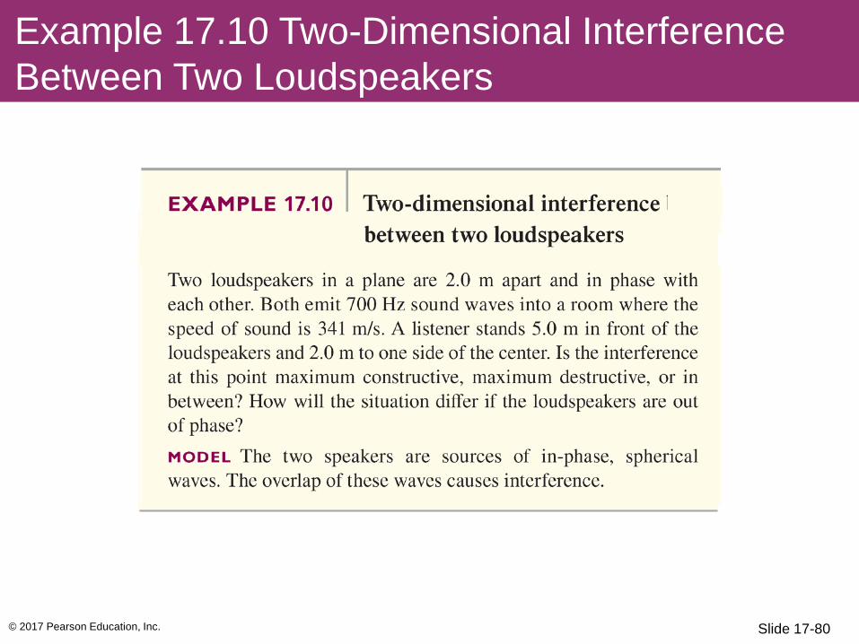
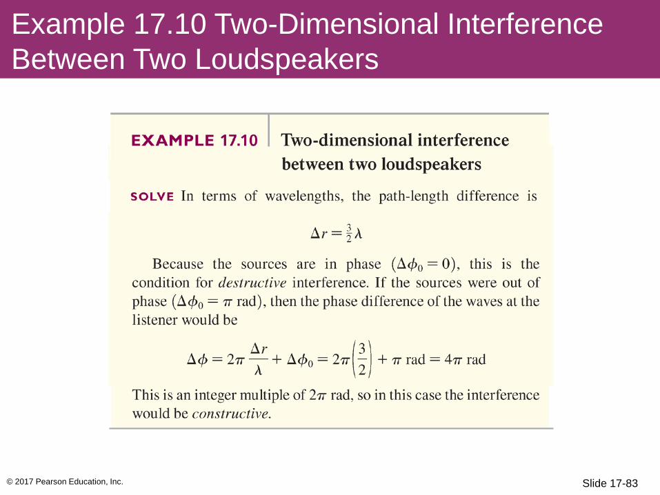
Example 17.10 Two-Dimensional Interference Between Two Loudspeakers
Slide 17-80

© 2017 Pearson Education, Inc.
Example 17.10 Two-Dimensional Interference Between Two Loudspeakers
Slide 17-81

© 2017 Pearson Education, Inc.
Example 17.10 Two-Dimensional Interference Between Two Loudspeakers
Slide 17-82
© 2017 Pearson Education, Inc.
Example 17.10 Two-Dimensional Interference Between Two Loudspeakers
Slide 17-83

© 2017 Pearson Education, Inc.
Example 17.10 Two-Dimensional Interference Between Two Loudspeakers
Slide 17-84
© 2017 Pearson Education, Inc.
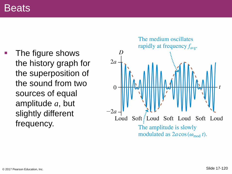
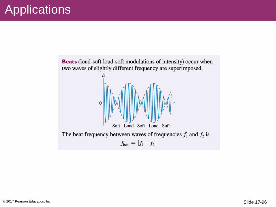
The figure shows the history graph for the superposition of the sound from two sources of equal amplitude a, but slightly different frequency.
Beats
Slide 17-120
© 2017 Pearson Education, Inc.
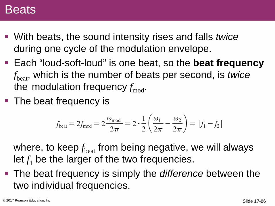
With beats, the sound intensity rises and falls twice during one cycle of the modulation envelope.
Each “loud-soft-loud” is one beat, so the beat frequency fbeat, which is the number of beats per second, is twice the modulation frequency fmod.
The beat frequency is
where, to keep fbeat from being negative, we will always let f1 be the larger of the two frequencies.
The beat frequency is simply the difference between the two individual frequencies.
Beats
Slide 17-86
© 2017 Pearson Education, Inc.
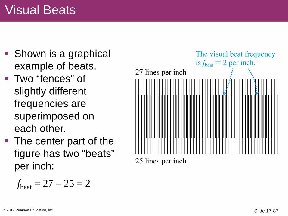
Shown is a graphical example of beats.
Two “fences” of slightly different frequencies are superimposed on each other.
The center part of the figure has two “beats” per inch:
Visual Beats
fbeat = 27 – 25 = 2
Slide 17-87

© 2017 Pearson Education, Inc.
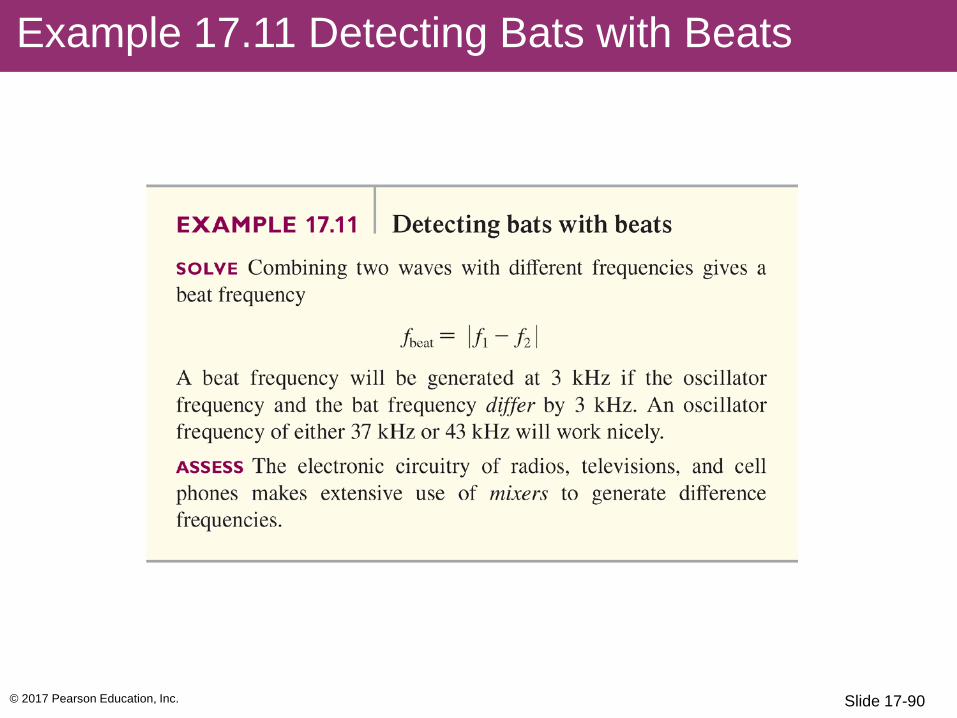
Example 17.11 Detecting Bats with Beats
Slide 17-88
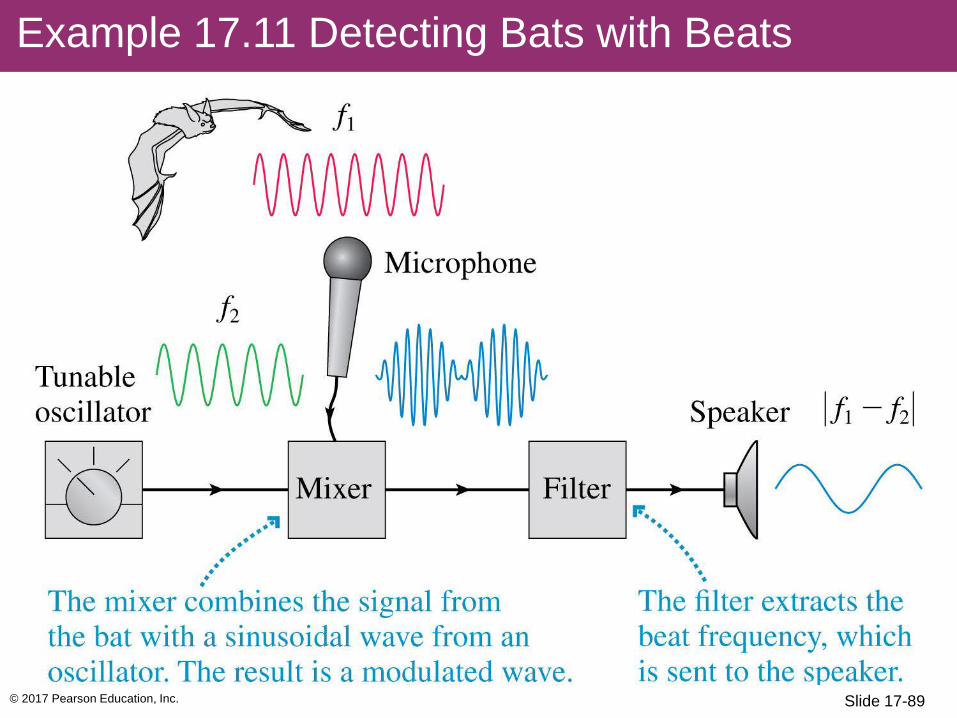
© 2017 Pearson Education, Inc.
Example 17.11 Detecting Bats with Beats
Slide 17-89
© 2017 Pearson Education, Inc.
Example 17.11 Detecting Bats with Beats
Slide 17-90

© 2017 Pearson Education, Inc.
Chapter 17 Summary Slides
Slide 17-91
© 2017 Pearson Education, Inc.
General Principles
Slide 17-92

© 2017 Pearson Education, Inc.
Important Concepts
Slide 17-93
© 2017 Pearson Education, Inc.
Important Concepts
Slide 17-94
© 2017 Pearson Education, Inc.
Applications
Slide 17-131 Slide 17-95
© 2017 Pearson Education, Inc.
Applications
Slide 17-96
Related Documents

![AH8-HC6 Lecture Chapter 17 - CISD ch 17.pdfMicrosoft PowerPoint - AH8-HC6 Lecture Chapter 17 [Compatibility Mode] Author: bford Created Date: 5/2/2018 11:12:17 AM ...](https://static.cupdf.com/doc/110x72/5f686ecdab24d17307391da0/ah8-hc6-lecture-chapter-17-cisd-ch-17pdf-microsoft-powerpoint-ah8-hc6-lecture.jpg)