Capital Structure Decisions: Extensions A t a meeting of the Financial Man- agement Association, a panel ses- sion focused on how firms actually set their target capital structures. The par- ticipants included financial managers from Hershey Foods, Verizon, EG&G (a high-tech firm), and a number of other firms in vari- ous industries. Although there were minor differences in philosophy and procedures among the companies, several themes emerged. First, in practice it is difficult to specify an optimal capital structure—indeed, managers even feel uncomfortable about specifying an optimal capital structure range. Thus, finan- cial managers worry primarily about whether their firms are using too little or too much debt, not about the precise optimal amount of debt. Second, even if a firm’s actual capital structure varies widely from the theoretical optimum, this might not have much effect on its stock price. Overall, financial managers believe that capital structure decisions are sec- ondary in importance to operating decisions, especially those relating to capital budgeting and the strategic direction of the firm. In general, financial managers focus on identifying a “prudent” level of debt rather than on setting a precise optimal level. A prudent level is defined as one that captures most of the benefits of debt yet (1) keeps finan- cial risk at a manageable level, (2) ensures future financing flexibility, and (3) allows the firm to maintain a desirable credit rating. Thus, a prudent level of debt will protect the company against financial distress under all but the worst economic scenarios, and it will ensure access to money and capital markets under most conditions. As you read this chapter, think about how you would make capital structure deci- sions if you had that responsibility. At the same time, don’t forget the very important message from the FMA panel session: Establishing the right capital structure is an imprecise process at best, and it should be based on both informed judgment and quantitative analyses. chapter 17

Welcome message from author
This document is posted to help you gain knowledge. Please leave a comment to let me know what you think about it! Share it to your friends and learn new things together.
Transcript

Capital Structure Decisions: Extensions
At a meeting of the Financial Man-
agement Association, a panel ses-
sion focused on how firms actually
set their target capital structures. The par-
ticipants included financial managers from
Hershey Foods, Verizon, EG&G (a high-tech
firm), and a number of other firms in vari-
ous industries. Although there were minor
differences in philosophy and procedures
among the companies, several themes
emerged.
First, in practice it is difficult to specify an
optimal capital structure—indeed, managers
even feel uncomfortable about specifying an
optimal capital structure range. Thus, finan-
cial managers worry primarily about whether
their firms are using too little or too much
debt, not about the precise optimal amount of
debt. Second, even if a firm’s actual capital
structure varies widely from the theoretical
optimum, this might not have much effect on
its stock price. Overall, financial managers
believe that capital structure decisions are sec-
ondary in importance to operating decisions,
especially those relating to capital budgeting
and the strategic direction of the firm.
In general, financial managers focus on
identifying a “prudent” level of debt rather
than on setting a precise optimal level. A
prudent level is defined as one that captures
most of the benefits of debt yet (1) keeps finan-
cial risk at a manageable level, (2) ensures
future financing flexibility, and (3) allows the
firm to maintain a desirable credit rating.
Thus, a prudent level of debt will protect the
company against financial distress under all
but the worst economic scenarios, and it will
ensure access to money and capital markets
under most conditions.
As you read this chapter, think about
how you would make capital structure deci-
sions if you had that responsibility. At the
same time, don’t forget the very important
message from the FMA panel session:
Establishing the right capital structure is an
imprecise process at best, and it should be
based on both informed judgment and
quantitative analyses.
chapter 17
Capital Structure Theory: Arbitrage Proofs of the Modigliani-Miller Models 607
The textbook’s Web sitecontains an Excel file thatwill guide you throughthe chapter’s calculations.The file for this chapter isFM12 Ch 17 Tool Kit.xls,and we encourage youto open the file and fol-low along as you readthe chapter.
1See Franco Modigliani and Merton H. Miller, “The Cost of Capital, Corporation Finance and the Theory of Investment,”American Economic Review, June 1958, pp. 261–297; “The Cost of Capital, Corporation Finance and the Theory ofInvestment: Reply,” American Economic Review, September 1958, pp. 655–669; “Taxes and the Cost of Capital: A Correction,” American Economic Review, June 1963, pp. 433–443; and “Reply,” American Economic Review, June1965, pp. 524–527. In a survey of Financial Management Association members, the original MM article was judgedto have had the greatest impact on the field of finance of any work ever published. See Philip L. Cooley and J. LouisHeck, “Significant Contributions to Finance Literature,” Financial Management, Tenth Anniversary Issue 1981, pp. 23–33. Note that both Modigliani and Miller won Nobel Prizes—Modigliani in 1985 and Miller in 1990.
Chapter 16 presented basic material on capital structure, including an introductionto capital structure theory. We saw that debt concentrates a firm’s business riskon its stockholders, thus raising stockholders’ risk, but it also increases theexpected return on equity. We also saw that there is some optimal level of debtthat maximizes a company’s stock price, and we illustrated this concept with asimple model. Now we go into more detail on capital structure theory. This willgive you a deeper understanding of the benefits and costs associated with debtfinancing.
17.1 Capital Structure Theory: Arbitrage Proofs of the Modigliani-Miller Models
Until 1958, capital structure theory consisted of loose assertions about investorbehavior rather than carefully constructed models that could be tested by formalstatistical analysis. In what has been called the most influential set of financialpapers ever published, Franco Modigliani and Merton Miller (MM) addressedcapital structure in a rigorous, scientific fashion, and they set off a chain ofresearch that continues to this day.1
Assumptions
As we explain in this chapter, MM employed the concept of arbitrage to developtheir theory. Arbitrage occurs if two similar assets—in this case, levered andunlevered stocks—sell at different prices. Arbitrageurs will buy the undervaluedstock and simultaneously sell the overvalued stock, earning a profit in the process,and this will continue until market forces of supply and demand cause the pricesof the two assets to be equal. For arbitrage to work, the assets must be equivalent,or nearly so. MM show that, under their assumptions, levered and unleveredstocks are sufficiently similar for the arbitrage process to operate.
No one, not even MM, believes that their assumptions are sufficiently correctto cause their models to hold exactly in the real world. However, their models doshow how money can be made through arbitrage if one can find ways aroundproblems with the assumptions. Here are the initial MM assumptions. Note thatsome of them were later relaxed:
1. There are no taxes, either personal or corporate.2. Business risk can be measured by �EBIT, and firms with the same degree of
business risk are said to be in a homogeneous risk class.3. All present and prospective investors have identical estimates of each firm’s
future EBIT; that is, investors have homogeneous expectations about expectedfuture corporate earnings and the riskiness of those earnings.
4. Stocks and bonds are traded in perfect capital markets. This assumption implies,among other things, (a) that there are no brokerage costs and (b) that investors(both individuals and institutions) can borrow at the same rate as corporations.
5. Debt is riskless. This applies to both firms and investors, so the interest rate onall debt is the risk-free rate. Further, this situation holds regardless of howmuch debt a firm (or individual) uses.
6. All cash flows are perpetuities; that is, all firms expect zero growth, hence have an“expectationally constant” EBIT, and all bonds are perpetuities. “Expectationallyconstant” means that the best guess is that EBIT will be constant, but after thefact the realized level could be different from the expected level.
MM without Taxes
MM first analyzed leverage under the assumption that there are no corporate orpersonal income taxes. On the basis of their assumptions, they stated and alge-braically proved two propositions:2
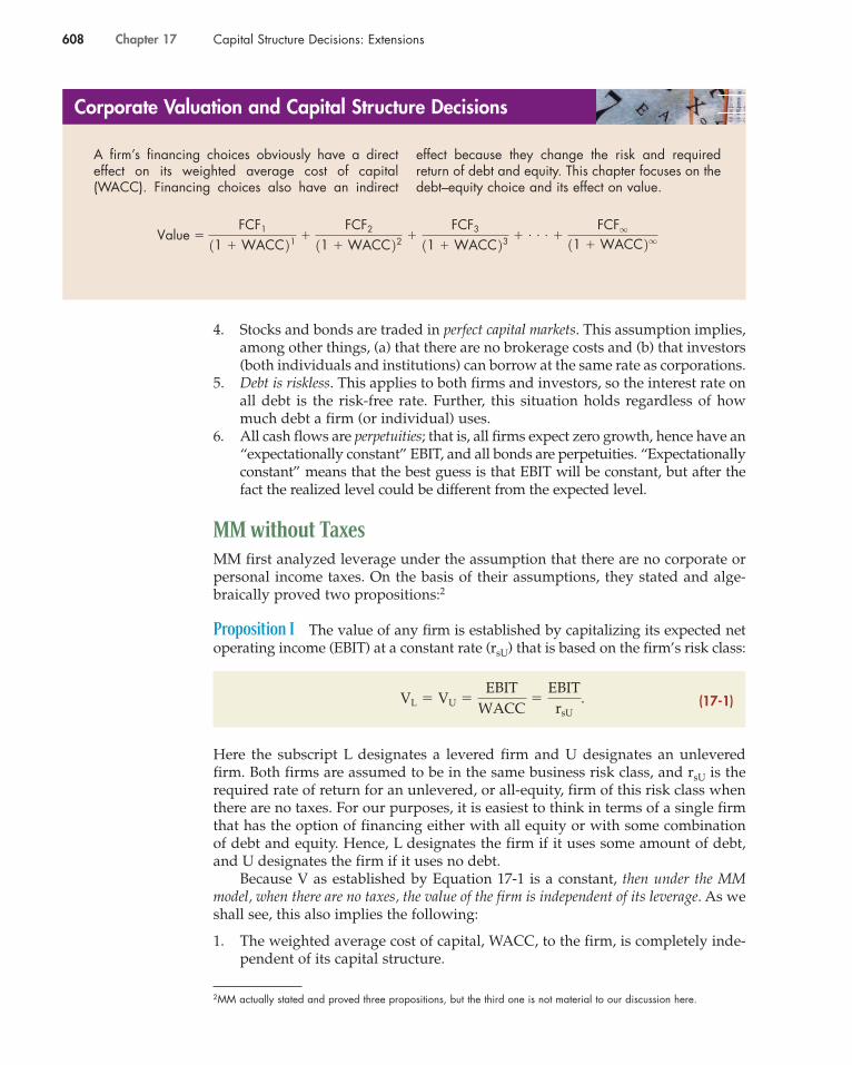
Proposition I The value of any firm is established by capitalizing its expected netoperating income (EBIT) at a constant rate (rsU) that is based on the firm’s risk class:
Here the subscript L designates a levered firm and U designates an unleveredfirm. Both firms are assumed to be in the same business risk class, and rsU is therequired rate of return for an unlevered, or all-equity, firm of this risk class whenthere are no taxes. For our purposes, it is easiest to think in terms of a single firmthat has the option of financing either with all equity or with some combinationof debt and equity. Hence, L designates the firm if it uses some amount of debt,and U designates the firm if it uses no debt.
Because V as established by Equation 17-1 is a constant, then under the MMmodel, when there are no taxes, the value of the firm is independent of its leverage. As weshall see, this also implies the following:
1. The weighted average cost of capital, WACC, to the firm, is completely inde-pendent of its capital structure.
VL � VU �EBIT
WACC�
EBIT
rsU
.
608 Chapter 17 Capital Structure Decisions: Extensions
2MM actually stated and proved three propositions, but the third one is not material to our discussion here.
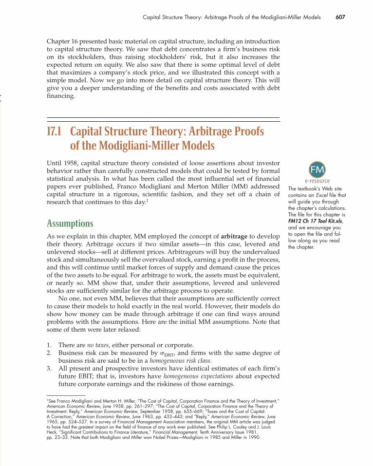
A firm’s financing choices obviously have a directeffect on its weighted average cost of capital(WACC). Financing choices also have an indirect
effect because they change the risk and requiredreturn of debt and equity. This chapter focuses on thedebt–equity choice and its effect on value.
Corporate Valuation and Capital Structure Decisions
Value �FCF1
11 � WACC 21 �FCF2
11 � WACC 22 �FCF3
11 � WACC 23 � . . . �FCF
q
11 � WACC 2q
(17-1)
Capital Structure Theory: Arbitrage Proofs of the Modigliani-Miller Models 609
2. Regardless of the amount of debt the firm uses, its WACC is equal to the costof equity that it would have if it used no debt.
Proposition II When there are no taxes, the cost of equity to a levered firm, rsL, isequal to (1) the cost of equity to an unlevered firm in the same risk class, rsU, plus(2) a risk premium whose size depends on both the difference between an unlevered firm’s costs of debt and equity and the amount of debt used:
Here D � market value of the firm’s debt, S � market value of its equity, and rd �
the constant cost of debt. Equation 17-2 states that as debt increases, the cost of equity alsorises, and in a mathematically precise manner (even though the cost of debt does not rise).
Taken together, the two MM propositions imply that using more debt in thecapital structure will not increase the value of the firm, because the benefits ofcheaper debt will be exactly offset by an increase in the riskiness of the equity,hence in its cost. Thus, MM argue that in a world without taxes, both the value of a firmand its WACC would be unaffected by its capital structure.
MM’s Arbitrage Proof
MM used an arbitrage proof to support their propositions.3 They showed that,under their assumptions, if two companies differed only (1) in the way they werefinanced and (2) in their total market values, then investors would sell shares ofthe higher-valued firm, buy those of the lower-valued firm, and continue thisprocess until the companies had exactly the same market value. To illustrate,assume that two firms, L and U, are identical in all important respects except thatFirm L has $4,000,000 of 7.5% debt while Firm U uses only equity. Both firms haveEBIT � $900,000, and �EBIT is the same for both firms, so they are in the same busi-ness risk class.
MM assumed that all firms are in a zero-growth situation; that is, EBIT isexpected to remain constant, which will occur if ROE is constant, all earnings arepaid out as dividends, and there are no taxes. Under the constant EBIT assump-tion, the total market value of the common stock, S, is the present value of a per-petuity, which is found as follows:
Equation 17-3 is merely the value of a perpetuity whose numerator is the netincome available to common stockholders, all of which is paid out as dividends,and whose denominator is the cost of common equity. Since there are no taxes, thenumerator is not multiplied by (1 � T) as it would be if we calculated NOPAT asin Chapters 3 and 15.
S �Dividends
rsL
�Net income
rsL
�
1EBIT � rdD 2rsL
.
rsL � rsU � Risk premium � rsU � 1rsU � rd 2 1D>S 2 .
3By arbitrage we mean the simultaneous buying and selling of essentially identical assets that sell at different prices.The buying increases the price of the undervalued asset, and the selling decreases the price of the overvalued asset.Arbitrage operations will continue until prices have adjusted to the point where the arbitrageur can no longer earn aprofit, at which point the market is in equilibrium. In the absence of transaction costs, equilibrium requires that theprices of the two assets be equal.
(17-2)
(17-3)

610 Chapter 17 Capital Structure Decisions: Extensions
Assume that initially, before any arbitrage occurs, both firms have the sameequity capitalization rate: rsU � rsL � 10%. Under this condition, according toEquation 17-3, the following situation would exist:
Firm U:
Firm L:
Thus before arbitrage, and assuming that rsU � rsL (which implies that capitalstructure has no effect on the cost of equity), the value of the levered Firm Lexceeds that of the unlevered Firm U.
MM argued that this is a disequilibrium situation that cannot persist. To seewhy, suppose you owned 10% of L’s stock, so the market value of your investmentwas 0.10($6,000,000) � $600,000. According to MM, you could increase yourincome without increasing your exposure to risk. For example, suppose you (1) sold your stock in L for $600,000, (2) borrowed an amount equal to 10% of L’s debt($400,000), and then (3) bought 10% of U’s stock for $900,000. Note that you wouldreceive $1,000,000 from the sale of your 10% of L’s stock plus your borrowing, andyou would be spending only $900,000 on U’s stock, so you would have an extra$100,000, which you could invest in riskless debt to yield 7.5%, or $7,500 annually.
Now consider your income positions:
� $10,000,000.
The total market value of Firm L � VL � DL � SL � $4,000,000 � $6,000,000
� $6,000,000.
�$900,000 � 0.0751$4,000,000 2
0.10�
$600,000
0.10
Value of Firm L’s stock � SL �EBIT � rdD
rsL
� $9,000,000.
The total market value of Firm U � VU � DU � SU � $0 � $9,000,000
�$900,000 � $0
0.10� $9,000,000.
Value of Firm U’s stock � SU �EBIT � rdD
rsU
Old Income: 10% of L’s $600,000 equity income $60,000
New Income: 10% of U’s $900,000 equity income $90,000
Less 7.5% interest on $400,000 loan (30,000) $60,000
Plus 7.5% interest on extra $100,000 7,500
Total new income $67,500
Capital Structure Theory: Arbitrage Proofs of the Modigliani-Miller Models 611
Thus, your net income from common stock would be exactly the same as before,$60,000, but you would have $100,000 left over for investment in riskless debt,which would increase your income by $7,500. Therefore, the total return on your$600,000 net worth would rise to $67,500. Further, your risk, according to MM,would be the same as before, because you would have simply substituted$400,000 of “homemade” leverage for your 10% share of Firm L’s $4 million of cor-porate leverage. Thus, neither your “effective” debt nor your risk would havechanged. Therefore, you would have increased your income without raising yourrisk, which is obviously a desirable thing to do.
MM argued that this arbitrage process would actually occur, with sales of L’sstock driving its price down and purchases of U’s stock driving its price up, untilthe market values of the two firms were equal. Until this equality was established,gains could be obtained by switching from one stock to the other; hence the profitmotive would force equality to be reached. When equilibrium is established, thevalues of Firms L and U, and their weighted average costs of capital, would beequal. Thus, according to Modigliani and Miller, both a firm’s value and its WACCmust be independent of capital structure.
Note that each of the assumptions listed at the beginning of this section is nec-essary for the arbitrage proof to work exactly. For example, if the companies didnot have identical business risk, or if transactions costs were significant, then thearbitrage process could not be invoked. We discuss other implications of theassumptions later in the chapter.
Arbitrage with Short Sales
Even if you did not own any stock in L, you still could reap benefits if U and L didnot have the same total market value. Your first step would be to sell short$600,000 of stock in L. To do this, your broker would let you borrow stock in Lfrom another client. Your broker would then sell the stock for you and give youthe proceeds, or $600,000 in cash. You would supplement this $600,000 by borrow-ing $400,000. With the $1 million total, you would buy 10% of the stock in U for$900,000, and have $100,000 remaining.
Your position would then consist of $100,000 in cash and two portfolios. Thefirst portfolio would contain $900,000 of stock in U, and it would generate $90,000of income. Because you own the stock, we’ll call it the “long” portfolio. The otherportfolio would consist of $600,000 of stock in L and $400,000 of debt. The valueof this portfolio is $1 million, and it would generate $60,000 of dividends and$30,000 of interest. However, you would not own this second portfolio—youwould “owe” it. Since you borrowed the $400,000, you would owe the $30,000 ininterest. And since you borrowed the stock in L, you would “owe the stock” to theclient from whom it was borrowed. Therefore, you would have to pay your bro-ker the $60,000 of dividends paid by L, which the broker would then pass on tothe client from whom the stock was borrowed. So, your net cash flow from the sec-ond portfolio would be a negative $90,000. Because you would “owe” this portfo-lio, we’ll call it the “short” portfolio.
Where would you get the $90,000 that you must pay on the short portfolio?The good news is that this is exactly the amount of cash flow generated by yourlong portfolio. Because the cash flows generated by each portfolio are the same,the short portfolio “replicates” the long portfolio.
Here is the bottom line. You started out with no money of your own. By sell-ing L short, borrowing $400,000, and purchasing stock in U, you ended up with$100,000 in cash plus the two portfolios. The portfolios mirror one another, so their

612 Chapter 17 Capital Structure Decisions: Extensions
net cash flow is zero. This is perfect arbitrage: You invest none of your ownmoney, you have no risk, you have no future negative cash flows, but you end upwith cash in your pocket.
Not surprisingly, many traders would want to do this. The selling pressure onL would cause its price to fall, and the buying pressure on U would cause its priceto rise, until the two companies’ values were equal. To put it another way, if thelong and short replicating portfolios have the same cash flows, then arbitrage will forcethem to have the same value.
This is one of the most important ideas in modern finance. Not only does itgive us insights into capital structure, but it is the fundamental building blockunderlying the valuation of real and financial options and derivatives as dis-cussed in Chapters 9 and 23. Without the concept of arbitrage, the options andderivatives markets we have today simply would not exist.
MM with Corporate Taxes
MM’s original work, published in 1958, assumed zero taxes. In 1963, they pub-lished a second article that incorporated corporate taxes. With corporate incometaxes, they concluded that leverage will increase a firm’s value. This occursbecause interest is a tax-deductible expense; hence more of a levered firm’s oper-ating income flows through to investors.
Later in this chapter we present a proof of the MM propositions when person-al taxes as well as corporate taxes are allowed. The situation when corporationsare subject to income taxes, but there are no personal taxes, is a special case of thesituation with both personal and corporate taxes, so we only present results here.
Proposition I The value of a levered firm is equal to the value of an unlevered firmin the same risk class (VU) plus the value of the tax shield (VTax shield) due to the taxdeductibility of interest expenses. The value of the tax shield, which is often calledthe gain from leverage, is the present value of the annual tax savings. The annual taxsaving is equal to the interest payment multiplied by the tax rate, T: Annual tax sav-ing � (rdT)(D). MM assume a no-growth firm, so the present value of the annual taxsaving is the present value of a perpetuity. They assume that the appropriate dis-count rate for the tax shield is the interest rate on debt, so the value of the tax shieldis VTax shield � (rdT)(D)/rd � TD. Therefore, the value of a levered firm is
The important point here is that when corporate taxes are introduced, the value ofthe levered firm exceeds that of the unlevered firm by the amount TD. Since thegain from leverage increases as debt increases, this implies that a firm’s value ismaximized at 100% debt financing.
Because all cash flows are assumed to be perpetuities, the value of the unlev-ered firm can be found by using Equation 17-3 and incorporating taxes. With zerodebt (D � $0), the value of the firm is its equity value:
VU � S �
EBIT11 � T 2rsU
.
� VU � TD.
VL � VU � VTax shield(17-4)
(17-5)
Capital Structure Theory: Arbitrage Proofs of the Modigliani-Miller Models 613
Note that the discount rate, rsU, is not necessarily equal to the discount rate inEquation 17-1. The rsU from Equation 17-1 is the required discount rate in a worldwith no taxes. The rsU in Equation 17-5 is the required discount rate in a worldwith taxes.
Proposition II The cost of equity to a levered firm is equal to (1) the cost of equityto an unlevered firm in the same risk class plus (2) a risk premium whose sizedepends on the difference between the costs of equity and debt to an unleveredfirm, the amount of financial leverage used, and the corporate tax rate:
Note that Equation 17-6 is identical to the corresponding without-tax equation, 17-2, except for the term (1 � T) in 17-6. Because (1 � T) is less than 1, corporatetaxes cause the cost of equity to rise less rapidly with leverage than it would in theabsence of taxes. Proposition II, coupled with the fact that taxes reduce the effec-tive cost of debt, is what produces the Proposition I result, namely, that the firm’svalue increases as its leverage increases.
As shown in Chapter 16, Professor Robert Hamada extended the MM analy-sis to define the relationship between a firm’s beta, b, and the amount of leverageit has. The beta of an unlevered firm is denoted by bU, and Hamada’s equation is
Note that beta, like the cost of stock shown in Equation 17-6, increases withleverage.
Illustration of the MM Models
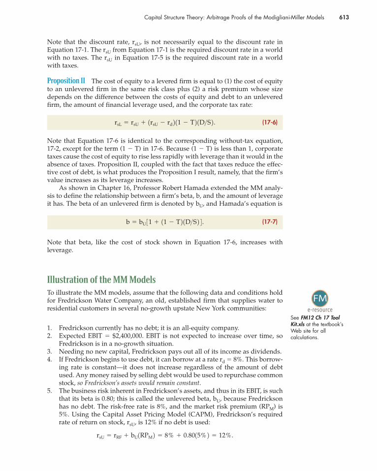
To illustrate the MM models, assume that the following data and conditions holdfor Fredrickson Water Company, an old, established firm that supplies water toresidential customers in several no-growth upstate New York communities:
1. Fredrickson currently has no debt; it is an all-equity company.2. Expected EBIT � $2,400,000. EBIT is not expected to increase over time, so
Fredrickson is in a no-growth situation.3. Needing no new capital, Fredrickson pays out all of its income as dividends.4. If Fredrickson begins to use debt, it can borrow at a rate rd � 8%. This borrow-
ing rate is constant—it does not increase regardless of the amount of debtused. Any money raised by selling debt would be used to repurchase commonstock, so Fredrickson’s assets would remain constant.
5. The business risk inherent in Fredrickson’s assets, and thus in its EBIT, is suchthat its beta is 0.80; this is called the unlevered beta, bU, because Fredricksonhas no debt. The risk-free rate is 8%, and the market risk premium (RPM) is5%. Using the Capital Asset Pricing Model (CAPM), Fredrickson’s requiredrate of return on stock, rsU, is 12% if no debt is used:
rsU � rRF � bU1RPM 2 � 8% � 0.8015% 2 � 12%.
b � bU 31 � 11 � T 2 1D>S 2 4 .
rsL � rsU � 1rsU � rd 2 11 � T 2 1D>S 2 .
See FM12 Ch 17 ToolKit.xls at the textbook’sWeb site for all calculations.
(17-6)
(17-7)

614 Chapter 17 Capital Structure Decisions: Extensions
With Zero Taxes To begin, assume that there are no taxes, so T � 0%. At any levelof debt, Proposition I (Equation 17-1) can be used to find Fredrickson’s value in anMM world, $20 million:
If Fredrickson uses $10 million of debt, its stock’s value must be $10 million:
We can also find Fredrickson’s cost of equity, rsL, and its WACC at a debt levelof $10 million. First, we use Proposition II (Equation 17-2) to find rsL, Fredrickson’slevered cost of equity:
Now we can find the company’s weighted average cost of capital:
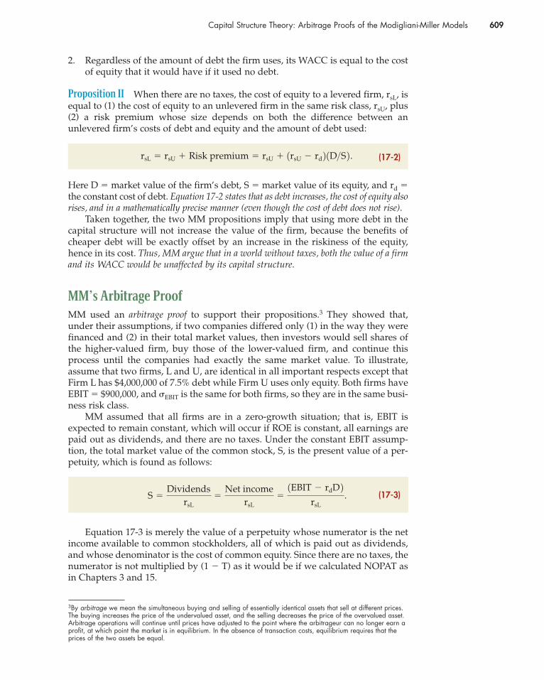
Fredrickson’s value and cost of capital based on the MM model without taxesat various debt levels are shown in Panel a on the left side of Figure 17-1. Here wesee that in an MM world without taxes, financial leverage simply does not matter:The value of the firm, and its overall cost of capital, are both independent of the amount of debt.
With Corporate Taxes To illustrate the MM model with corporate taxes, assumethat all of the previous conditions hold except these two:
1. Expected EBIT � $4,000,000.4
2. Fredrickson has a 40% federal-plus-state tax rate, so T � 40%.
Other things held constant, the introduction of corporate taxes would lowerFredrickson’s net income, hence its value, so we increased EBIT from $2.4 millionto $4 million to make the comparison between the two models easier.
When Fredrickson has zero debt but pays taxes, Equation 17-5 can be used tofind its value, $20 million:
VU �
EBIT11 � T 2rsU
�
$4 million10.6 20.12
� $20 million.
� 1$10>$20 2 18% 2 11.0 2 � 1$10>$20 2 116.0% 2 � 12.0%.
WACC � 1D>V 2 1rd 2 11 � T 2 � 1S>V 2rsL
� 12% � 4.0% � 16.0%.
� 12% � 112% � 8% 2 1$10 million>$10 million 2 rsL � rsU � 1rsU � rd 2 1D>S 2
S � V � D � $20 million � $10 million � $10 million.
VL � VU �EBIT
rsU
�$2.4 million
0.12� $20.0 million.
4If we had left Fredrickson’s EBIT at $2.4 million, the introduction of corporate taxes would have reduced the firm’svalue from $20 million to $12 million:
Corporate taxes reduce the amount of operating income available to investors in an unlevered firm by the factor (1 � T), so the value of the firm would be reduced by the same amount, holding rsU constant.
VU �
EBIT11 � T 2rsU
�
$2.4 million10.6 20.12
� $12.0 million.
Capital Structure Theory: Arbitrage Proofs of the Modigliani-Miller Models 615
V = 20
10
20
30
20 40 60 80 100
Cost of Capital(%)
0
Debt/Value Ratio (%)
WACC
rd
10
20
30
20 40 60 80 100
Cost of Capital(%)
0
Debt/Value Ratio (%)
rs
rs
WACC
r (1 – T)d
10
VU = 20
30
20
Value of Firm, V($)
0
Debt ($)
VL
10
30
5 33.30
b. With Corporate Taxesa. Without Taxes
15105
Value of Firm, V($)
Debt ($)
VUU
33.33 VL
10 15 20 25 30
TD
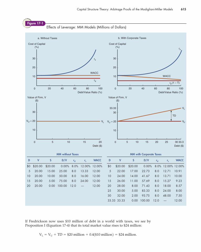
Effects of Leverage: MM Models (Millions of Dollars)Figure 17-1
MM without Taxes MM with Corporate Taxes
D V S D/V rd rs WACC D V S D/V rd rs WACC
$0 $20.00 $20.00 0.00% 8.0% 12.00% 12.00% $0 $20.00 $20.00 0.00% 8.0% 12.00% 12.00%
5 20.00 15.00 25.00 8.0 13.33 12.00 5 22.00 17.00 22.73 8.0 12.71 10.91
10 20.00 10.00 50.00 8.0 16.00 12.00 10 24.00 14.00 41.67 8.0 13.71 10.00
15 20.00 5.00 75.00 8.0 24.00 12.00 15 26.00 11.00 57.69 8.0 15.27 9.23
20 20.00 0.00 100.00 12.0 — 12.00 20 28.00 8.00 71.43 8.0 18.00 8.57
25 30.00 5.00 83.33 8.0 24.00 8.00
30 32.00 2.00 93.75 8.0 48.00 7.50
33.33 33.33 0.00 100.00 12.0 — 12.00
If Fredrickson now uses $10 million of debt in a world with taxes, we see byProposition I (Equation 17-4) that its total market value rises to $24 million:
VL � VU � TD � $20 million � 0.41$10 million 2 � $24 million.

616 Chapter 17 Capital Structure Decisions: Extensions
Therefore, the implied value of Fredrickson’s equity is $14 million:
We can also find Fredrickson’s cost of equity, rsL, and its WACC at a debt levelof $10 million. First, we use Proposition II (Equation 17-6) to find rsL, the leveredcost of equity:
The company’s weighted average cost of capital is 10%:
Note that we could also find the levered beta and then the levered cost of equity.First, we apply Hamada’s equation to find the levered beta:
Applying the CAPM, the levered cost of equity is
Notice that this is the same levered cost of equity that we obtained directly usingEquation 17-6.
Fredrickson’s value and cost of capital at various debt levels with corporatetaxes are shown in Panel b on the right side of Figure 17-1. In an MM world withcorporate taxes, financial leverage does matter: The value of the firm is maximized,and its overall cost of capital is minimized, if it uses almost 100% debt financing.The increase in value is due solely to the tax deductibility of interest payments,which lowers both the cost of debt and the equity risk premium by (1 � T).5
rsL � rRF � b1RPM 2 � 8% � 1.142915% 2 � 0.1371 � 13.71%.
� 1.1429.
� 0.80 31 � 11 � 0.4 2 1$10 million>$14 million 2 4 b � bU 31 � 11 � T 2 1D>S 2 4
� 1$10>$24 2 18% 2 10.6 2 � 1$14>$24 2 113.71% 2 � 10.0%.
WACC � 1D>V 2 1rd 2 11 � T 2 � 1S>V 2rsL
� 12% � 1.71% � 13.71%.
� 12% � 112% � 8% 2 10.6 2 1$10 million>$14 million 2 rsL � rsU � 1rsU � rd 2 11 � T 2 1D>S 2
S � V � D � $24 million � $10 million � $14 million.
5In the limiting case, where the firm used 100% debt financing, the bondholders would own the entire company;thus, they would have to bear all the business risk. (Up until this point, MM assume that the stockholders bear all therisk.) If the bondholders bear all the risk, then the capitalization rate on the debt should be equal to the equity capi-talization rate at zero debt, rd � rsU � 12%.
The income stream to the stockholders in the all-equity case was $4,000,000(1 � T) � $2,400,000, and thevalue of the firm was
With all debt, the entire $4,000,000 of EBIT would be used to pay interest charges—rd would be 12%, so I � 0.12(Debt) � $4,000,000. Taxes would be zero, and investors (bondholders) would get the entire $4,000,000 of operating income; they would not have to share it with the government. Thus, at 100% debt, the value of the firmwould be
There is, of course, a transition problem in all this—MM assume that rd � 8% regardless of how much debt the firmhas until debt reaches 100%, at which point rd jumps to 12%, the cost of equity. As we shall see later in the chapter,rd realistically rises as the use of financial leverage increases.
VL �$4,000,000
0.12� $33,333,333 � D.
VU �$2,400,000
0.12� $20,000,000.
Introducing Personal Taxes: The Miller Model 617
To conclude this section, compare the “Without Taxes” and “With CorporateTaxes” sections of Figure 17-1. Without taxes, both WACC and the firm’s value (V)are constant. With corporate taxes, WACC declines and V rises as more and moredebt is used, so the optimal capital structure, under MM with corporate taxes, is100% debt.
6See Merton H. Miller, “Debt and Taxes,” Journal of Finance, May 1977, pp. 261–275.
17.2 Introducing Personal Taxes: The Miller Model
Although MM included corporate taxes in the second version of their model, theydid not extend the model to include personal taxes. However, in his presidentialaddress to the American Finance Association, Merton Miller presented a model toshow how leverage affects firms’ values when both personal and corporate taxesare taken into account.6 To explain Miller’s model, we begin by defining Tc as thecorporate tax rate, Ts as the personal tax rate on income from stocks, and Td as thepersonal tax rate on income from debt. Note that stock returns are expected tocome partly as dividends and partly as capital gains, so Ts is a weighted averageof the effective tax rates on dividends and capital gains. However, essentially alldebt income comes from interest, which is effectively taxed at investors’ top rates,so Td is higher than Ts.
With personal taxes included, and under the same set of assumptions used inthe earlier MM models, the value of an unlevered firm is found as follows:
The (1 � Ts) term takes account of personal taxes. Note that to find the value of the unlevered firm we can either discount pre-personal-tax cash flows at the pre-personal-tax rate of rsU or the after-personal-tax cash flows at the after-personal-taxrate of rsU(1 � Ts). Therefore, the numerator of the second form of Equation 17-8shows how much of the firm’s operating income is left after the unlevered firmpays corporate income taxes and its stockholders subsequently pay personal taxeson their equity income. Note also that the discount rate, rsU, in Equation 17-8 is not
VU �
EBIT11 � Tc 2rsU
�
EBIT11 � Tc 2 11 � Ts 2rsU11 � Ts 2 .
Is there an optimal capital structure under the MM zero-tax model?
What is the optimal capital structure under the MM model with corporate taxes?
How does the Proposition I equation differ between the two models?
How does the Proposition II equation differ between the two models?
Why do taxes result in a “gain from leverage” in the MM model with corporate taxes?
An unlevered firm has a value of $100 million. An otherwise identical but levered firm has $30 million in debt. Under the MM zero-tax model, what is the value of the levered firm? Under the MMcorporate tax model, what is the value of a levered firm if the corporate tax rate is 40%? ($100 million;$112 million)
SELF-TEST
(17-8)
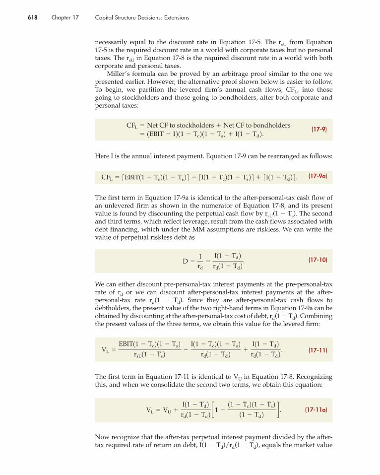
necessarily equal to the discount rate in Equation 17-5. The rsU from Equation 17-5 is the required discount rate in a world with corporate taxes but no personaltaxes. The rsU in Equation 17-8 is the required discount rate in a world with bothcorporate and personal taxes.
Miller’s formula can be proved by an arbitrage proof similar to the one wepresented earlier. However, the alternative proof shown below is easier to follow.To begin, we partition the levered firm’s annual cash flows, CFL, into those going to stockholders and those going to bondholders, after both corporate andpersonal taxes:
Here I is the annual interest payment. Equation 17-9 can be rearranged as follows:
The first term in Equation 17-9a is identical to the after-personal-tax cash flow ofan unlevered firm as shown in the numerator of Equation 17-8, and its presentvalue is found by discounting the perpetual cash flow by rsU(1 � Ts). The secondand third terms, which reflect leverage, result from the cash flows associated withdebt financing, which under the MM assumptions are riskless. We can write thevalue of perpetual riskless debt as
We can either discount pre-personal-tax interest payments at the pre-personal-taxrate of rd or we can discount after-personal-tax interest payments at the after-personal-tax rate rd(1 � Td). Since they are after-personal-tax cash flows todebtholders, the present value of the two right-hand terms in Equation 17-9a can beobtained by discounting at the after-personal-tax cost of debt, rd(1 � Td). Combiningthe present values of the three terms, we obtain this value for the levered firm:
The first term in Equation 17-11 is identical to VU in Equation 17-8. Recognizingthis, and when we consolidate the second two terms, we obtain this equation:
Now recognize that the after-tax perpetual interest payment divided by the after-tax required rate of return on debt, I(1 � Td)/rd(1 � Td), equals the market value
VL � VU �
I11 � Td 2rd11 � Td 2 c1 �
11 � Tc 2 11 � Ts 211 � Td 2 d .
VL �
EBIT11 � Tc 2 11 � Ts 2rsU11 � Ts 2 �
I11 � Tc 2 11 � Ts 2rd11 � Td 2 �
I11 � Td 2rd11 � Td 2 .
D �I
rd
�
I11 � Td 2rd11 � Td 2 .
CFL � 3EBIT11 � Tc 2 11 � Ts 2 4 � 3I11 � Tc 2 11 � Ts 2 4 � 3I11 � Td 2 4 .
� 1EBIT � I 2 11 � Tc 2 11 � Ts 2 � I11 � Td 2 . CFL � Net CF to stockholders � Net CF to bondholders
618 Chapter 17 Capital Structure Decisions: Extensions
(17-9)
(17-9a)
(17-10)
(17-11a)
(17-11)

of the debt, D. Substituting D into the preceding equation and rearranging, weobtain this expression, called the Miller model:
The Miller model provides an estimate of the value of a levered firm in a worldwith both corporate and personal taxes.
The Miller model has several important implications:
1. The term in brackets,
when multiplied by D, represents the gain from leverage. The bracketed termthus replaces the corporate tax rate, T, in the earlier MM model with corporatetaxes, VL � VU � TD.
2. If we ignore all taxes, that is, if Tc � Ts � Td � 0, then the bracketed term iszero, so in that case Equation 17-12 is the same as the original MM modelwithout taxes.
3. If we ignore personal taxes, that is, if Ts � Td � 0, then the bracketed termreduces to [1 � (1 � Tc)] � Tc, so Equation 17-12 is the same as the MM modelwith corporate taxes.
4. If the effective personal tax rates on stock and bond incomes were equal, thatis, if Ts � Td, then (1 � Ts) and (1 � Td) would cancel, and the bracketed termwould again reduce to Tc.
5. If (1 � Tc)(1 � Ts) � (1 � Td), then the bracketed term would be zero, and thevalue of using leverage would also be zero. This implies that the tax advantageof debt to the firm would be exactly offset by the personal tax advantage of equi-ty. Under this condition, capital structure would have no effect on a firm’s valueor its cost of capital, so we would be back to MM’s original zero-tax theory.
6. Because taxes on capital gains are lower than on ordinary income and can bedeferred, the effective tax rate on stock income is normally less than that onbond income. This being the case, what would the Miller model predict as thegain from leverage? To answer this question, assume that the tax rate on cor-porate income is Tc � 34%, the effective rate on bond income is Td � 28%, andthe effective rate on stock income is Ts � 15%.7 Using these values in theMiller model, we find that a levered firm’s value exceeds that of an unleveredfirm by 22% of the market value of corporate debt:
� 0.22D.
� 11 � 0.78 2D � c1 �
11 � 0.34 2 11 � 0.15 211 � 0.28 2 dD
Gain from leverage � c1 �
11 � Tc 2 11 � Ts 211 � Td 2 dD
c1 �
11 � Tc 2 11 � Ts 211 � Td 2 d ,
Miller model: VL � VU � c1 �
11 � Tc 2 11 � Ts 211 � Td 2 dD.
Introducing Personal Taxes: The Miller Model 619
7In a 1978 article, Miller and Scholes described how investors could, theoretically, shelter or delay income fromstock to the point where the effective personal tax rate on such income is essentially zero. See Merton H. Millerand Myron S. Scholes, “Dividends and Taxes,” Journal of Financial Economics, December 1978, pp. 333–364.However, the 1986 changes in the tax law eliminated most of the shelters Miller and Scholes discussed.
(17-12)
620 Chapter 17 Capital Structure Decisions: Extensions
Note that the MM model with corporate taxes would indicate a gain from lever-age of Tc(D) � 0.34D, or 34% of the amount of corporate debt. Thus, with theseassumed tax rates, adding personal taxes to the model lowers but does not eliminatethe benefit from corporate debt. In general, whenever the effective tax rate on incomefrom stock is less than the effective rate on income from bonds, the Miller model pro-duces a lower gain from leverage than is produced by the MM with-tax model.
In his paper, Miller argued that firms in the aggregate would issue a mix ofdebt and equity securities such that the before-tax yields on corporate securitiesand the personal tax rates of the investors who bought these securities wouldadjust until an equilibrium was reached. At equilibrium, (1 � Td) would equal (1 � Tc)(1 � Ts), so, as we noted earlier in point 5, the tax advantage of debt to thefirm would be exactly offset by personal taxation, and capital structure would haveno effect on a firm’s value or its cost of capital. Thus, according to Miller, the con-clusions derived from the original Modigliani-Miller zero-tax model are correct!
Others have extended and tested Miller’s analysis. Generally, these extensionsquestion Miller’s conclusion that there is no advantage to the use of corporate debt.In fact, Equation 17-12 shows that both Tc and Ts must be less than Td if there is to bezero gain from leverage. In the United States, for most corporations and investors,the effective tax rate on income from stock is less than on income from bonds; that is,Ts � Td. However, many corporate bonds are held by tax-exempt institutions, and inthose cases Tc is generally greater than Td. Also, for those high-tax-bracket individu-als with Td � Tc, Ts may be large enough so that (1 � Tc)(1 � Ts) is less than (1 � Td);hence there is an advantage to the use of corporate debt. Still, Miller’s work doesshow that personal taxes offset some of the benefits of corporate debt, so the taxadvantages of corporate debt are less than were implied by the earlier MM model,where only corporate taxes were considered.
As we note in the next section, both the MM and the Miller models are basedon strong and unrealistic assumptions, so we should regard our examples as indi-cating the general effects of leverage on a firm’s value, not a precise relationship.
How does the Miller model differ from the MM model with corporate taxes?
What are the implications of the Miller model if Tc � Ts � Td � 0?
What are the implications if Ts � Td � 0?
Considering the current tax structure in the United States, what is the primary implication of the Millermodel?
An unlevered firm has a value of $100 million. An otherwise identical but levered firm has $30 millionin debt. Under the Miller model, what is the value of a levered firm if the corporate tax rate is 40%, thepersonal tax rate on equity is 15%, and the personal tax rate on debt is 35%? ($106.46 million)
SELF-TEST
17.3 Criticisms of the MM and Miller Models
The conclusions of the MM and Miller models follow logically from their initialassumptions. However, both academicians and executives have voiced concernsover the validity of the MM and Miller models, and virtually no one believes they hold precisely. The MM zero-tax model leads to the conclusion that capitalstructure doesn’t matter, yet we observe systematic capital structure patternswithin industries. Further, when used with “reasonable” tax rates, both the MMmodel with corporate taxes and the Miller model lead to the conclusion that firmsshould use 100% debt financing, but firms do not (deliberately) go to that extreme.
Criticisms of the MM and Miller Models 621
People who disagree with the MM and Miller theories generally attack themon the grounds that their assumptions are not correct. Here are the main objections:
1. Both MM and Miller assume that personal and corporate leverage are perfectsubstitutes. However, an individual investing in a levered firm has less lossexposure as a result of corporate limited liability than if he or she used “home-made” leverage. For example, in our earlier illustration of the MM arbitrageargument, it should be noted that only the $600,000 our investor had in Firm Lwould be lost if that firm went bankrupt. However, if the investor engaged inarbitrage transactions and employed “homemade” leverage to invest in FirmU, then he or she could lose $900,000—the original $600,000 investment plusthe $400,000 loan less the $100,000 investment in riskless bonds. Thisincreased personal risk exposure would tend to restrain investors from engag-ing in arbitrage, and that could cause the equilibrium values of VL, VU, rsL, andrsU to be different from those specified by MM. Restrictions on institutionalinvestors, who dominate capital markets today, may also retard the arbitrageprocess, because many institutional investors cannot legally borrow to buystocks, hence are prohibited from engaging in homemade leverage.
Note, though, that while limited liability may present a problem toindividuals, it does not present a problem to corporations set up to undertakeleveraged buyouts (LBOs). Thus, after MM’s work became widely known,literally hundreds of LBO firms were established, and their founders madebillions recapitalizing underleveraged firms. “Junk bonds” were created toaid in the process, and the managers of underleveraged firms who did notwant their firms to be taken over increased debt usage on their own. Thus,MM’s work raised the level of debt in corporate America, and that probablyraised the level of economic efficiency.
2. If a levered firm’s operating income declined, it would sell assets and takeother measures to raise the cash necessary to meet its interest obligations andthus avoid bankruptcy. If our illustrative unlevered firm experienced thesame decline in operating income, it would probably take the less drasticmeasure of cutting dividends rather than selling assets. If dividends were cut,investors who employed homemade leverage would not receive cash to paythe interest on their debt. Thus, homemade leverage puts stockholders ingreater danger of bankruptcy than does corporate leverage.
3. Brokerage costs were assumed away by MM and Miller, making the switchfrom L to U costless. However, brokerage and other transaction costs do exist,and they too impede the arbitrage process.
4. MM initially assumed that corporations and investors can borrow at the risk-free rate. Although risky debt has been introduced into the analysis by others,to reach the MM and Miller conclusions it is still necessary to assume thatboth corporations and investors can borrow at the same rate. While majorinstitutional investors probably can borrow at the corporate rate, many insti-tutions are not allowed to borrow to buy securities. Further, most individualinvestors must borrow at higher rates than those paid by large corporations.
5. In his article, Miller concluded that an equilibrium would be reached, but toreach his equilibrium the tax benefit from corporate debt must be the same forall firms, and it must be constant for an individual firm regardless of theamount of leverage used. However, we know that tax benefits vary from firmto firm: Highly profitable companies gain the maximum tax benefit fromleverage, while the benefits to firms that are struggling are much smaller.Further, some firms have other tax shields such as high depreciation, pension
622 Chapter 17 Capital Structure Decisions: Extensions
plan contributions, and operating loss carryforwards, and these shields reducethe tax savings from interest payments.8 It also appears simplistic to assumethat the expected tax shield is unaffected by the amount of debt used. Higherleverage increases the probability that the firm will not be able to use the fulltax shield in the future, because higher leverage increases the probability offuture unprofitability and consequently lower tax rates. Note also that large,diversified corporations can use losses in one division to offset profits inanother. Thus, the tax shelter benefit is more certain in large, diversified firmsthan in smaller, single-product companies. All things considered, it appearslikely that the interest tax shield from corporate debt is more valuable to somefirms than to others.
6. MM and Miller assume that there are no costs associated with financial distress,and they ignore agency costs. Further, they assume that all market participantshave identical information about firms’ prospects, which is also incorrect.
These six points all suggest that the MM and Miller models lead to questionableconclusions, and that the models would be better if certain of their assumptionscould be relaxed. We discuss an extension of the models in the next section.
8For a discussion of the impact of tax shields, see Harry DeAngelo and Ronald W. Masulis, “Optimal CapitalStructure under Corporate and Personal Taxation,” Journal of Financial Economics, March 1980, pp. 3–30; ThomasW. Downs, “Corporate Leverage and Nondebt Tax Shields: Evidence on Crowding-Out,” The Financial Review,November 1993, pp. 549–583; John R. Graham, “Taxes and Corporate Finance: A Review,” The Review ofFinancial Studies, Winter 2003, pp. 1075–1129; Moshe Ben-Horim, Shalom Hochman, and Oded Palmon, “TheImpact of the 1986 Tax Reform Act on Corporate Financial Policy,” Financial Management, Autumn 1987, pp. 29–35; Jeffrey K. Mackie-Mason, “Do Taxes Affect Corporate Financing Decisions?” Journal of Finance,December 1990, pp. 1471–1493; John M. Harris, Jr., Rodney L. Roenfeldt, and Philip L. Cooley, “Evidence ofFinancial Leverage Clienteles,” Journal of Finance, September 1983, pp. 1125–1132; and Josef Zechner, “TaxClienteles and Optimal Capital Structure under Uncertainty,” Journal of Business, October 1990, pp. 465–491.9See Phillip R. Daves and Michael C. Ehrhardt, “Corporate Valuation: The Combined Impact of Growth and the TaxShield of Debt on the Cost of Capital and Systematic Risk,” Journal of Applied Finance, Fall/Winter 2002, pp. 31–38.
Should we accept that one of the models presented thus far (MM with zero taxes, MM with corporatetaxes, or Miller) is correct? Why or why not?
Are any of the assumptions used in the models worrisome to you, and what does “worrisome” mean inthis context?
SELF-TEST
17.4 An Extension to the MM Model: Nonzero Growth and a Risky Tax Shield
In this section we discuss an extension to the MM model that incorporates growthand different discount rates for the debt tax shield.9
MM assumed that firms pay out all of their earnings as dividends and there-fore do not grow. However, most firms do grow, and growth affects the MM andHamada results (as found in the first part of this chapter). Recall that for an unlev-ered firm, the WACC is just the unlevered cost of equity: WACC � rsU. If g is theconstant growth rate and FCF is the expected free cash flow, then the corporatevalue model from Chapter 15 shows that
VU �FCF
rsU � g. (17-13)
An Extension to the MM Model: Nonzero Growth and a Risky Tax Shield 623
As shown by Equation 17-4, the value of the levered firm is equal to the value ofthe unlevered firm plus gain from leverage, which is the value of the tax shield:
However, when there is growth, the value of the tax shield is not equal to TD as itis in the MM model with corporate taxes. If the firm uses debt and g is positive,then, as the firm grows, the amount of debt will increase over time; hence the sizeof the annual tax shield will also increase at the rate g, provided the debt ratioremains constant. Moreover, the value of this growing tax shield is greater thanthe value of the constant tax shield in the MM analysis.
MM assumed that corporate debt was riskless and that the firm would alwaysbe able to use its tax savings. Therefore, they discounted the tax savings at the costof debt, rd, which is the risk-free rate. However, corporate debt is not risk free—firms do occasionally default on their loans. Also, a firm may not be able to usetax savings from debt in the current year if it already has a pre-tax loss from oper-ations. Therefore, the flow of tax savings to the firm is not risk free; hence it shouldbe discounted at a rate greater than the risk-free rate. In addition, since debt is saferthan equity to an investor because it has a higher priority claim on the firm’s cashflows, its discount rate should be no greater than the unlevered cost of equity. Fornow, assume that the appropriate discount rate for the tax savings is rTS, which isgreater than or equal to the cost of debt, rd, and less than or equal to the unleveredcost of equity, rsU.
If rTS is the appropriate discount rate for the tax shield, rd is the interest rateon the debt, T is the corporate tax rate, and D is the current amount of debt, thenthe present value of this growing tax shield is
This formula is the same as the dividend growth formula from Chapter 8, with rdTD as the growing cash flow generated by the tax savings. SubstitutingEquation 17-14 into 17-4a provides a valuation equation that incorporatesconstant growth:
The difference between Equation 17-15 for the value of the levered firm and theexpression given in Equation 17-4 is the rd/(rTS � g) term in parentheses, whichreflects the added value of the tax shield due to growth. In the MM model, rTS �
rd � rRF and g � 0 so the term in parentheses is equal to 1.0.If rTS � rsU, growth can actually cause the levered cost of equity to be less than
the unlevered cost of equity.10 This happens because the combination of rapidgrowth and a low discount rate for the tax shield causes the value of the tax shieldto dominate the unlevered value of the firm. If this were true, then high-growth
VL � VU � a rd
rTS � gbTD.
VTax shield �rdTD
rTS � g.
VL � VU � VTax shield.
10See the paper by Daves and Ehrhardt in Footnote 9.
(17-14)
(17-15)
(17-4a)
624 Chapter 17 Capital Structure Decisions: Extensions
firms would tend to have larger amounts of debt than low-growth firms.However, this isn’t consistent with either intuition or what we observe in the mar-ket: High-growth firms actually tend to have lower levels of debt. Regardless ofthe growth rate, firms with more debt should have a higher cost of equity thanfirms with no debt. These inconsistencies can be prevented if rTS � rsU. With thisresult, the value of the levered firm becomes11
Based on this valuation equation, the expressions for the levered cost of equity and the levered beta that correspond to Equations 17-6 and 17-7 are
and
As in Chapter 16, bU is the beta of an unlevered firm and b is the beta of a leveredfirm. Because debt is not riskless, it has a beta, bD.
Although the derivations of Equations 17-17 and 17-18 reflect corporate taxesand growth, neither of these expressions has the corporate tax rate or the growthrate in it. This means the expression for the levered required rate of return, Equation17-17, is exactly the same as MM’s expression for the levered required rate of returnwithout taxes, Equation 17-2. And the expression for the levered beta, Equation 17-18, is exactly the same as Hamada’s equation (with risky debt), but without taxes.The reason the tax rate and the growth rate drop out of these two expressions is thatthe growing tax shield is discounted at the unlevered cost of equity, rsU, not at thecost of debt as in the MM model. The tax rate drops out because no matter how highthe level of T, the total risk of the firm will not be changed since the unlevered cashflows and the tax shield are discounted at the same rate. The growth rate drops outfor the same reason: An increasing debt level will not change the riskiness of theentire firm no matter what rate of growth prevails.12
Note that Equation 17-18 has the expression bD. Since MM and Hamadaassumed that corporate debt is riskless, its beta should be zero. However, ifcorporate debt is not riskless, then its beta, bD, may not be zero. Assuming bondslie on the Security Market Line, a bond’s required return, rd, can be expressed as rd � rRF � bDRPM. Solving for bD gives bD � (rd � rRF)/RPM.
b � bU � 1bU � bD 2DS .
rsL � rsU � 1rsU � rd 2DS
VL � VU �rdTD
rsU � g.
11See Steven N. Kaplan and Richard S. Ruback, “The Valuation of Cash Flow Forecasts: An Empirical Analysis,”Journal of Finance, September 1995, pp. 1059–1093, for a discussion of the compressed APV valuation method,which uses the assumption that rTS � rsU.12Of course Equations 17-14, 17-15, and 17-16 also apply to firms that don’t happen to be growing. In this specialcase, the difference between the Ehrhardt and Daves extension and the MM with taxes treatment is that MM assumethat the tax shield should be discounted at the risk-free rate, while this extension to their model shows that it is morereasonable for the tax shield to be discounted at the unlevered cost of equity, rsU. Because rsU is greater than the risk-free rate, the value of a nongrowing tax shield will be lower when discounted at this higher rate, giving a lowervalue of the levered firm than what MM would predict.
(17-16)
(17-17)
(17-18)
An Extension to the MM Model: Nonzero Growth and a Risky Tax Shield 625
Illustration of the MM Extension with Growth
Earlier in this chapter we examined Fredrickson Water Company, a zero-growthfirm with unlevered value of $20 million. To see how growth affects the leveredvalue of the firm and the levered cost of equity, let’s look at Peterson Power Inc.,which is similar to Fredrickson, except that it is growing. Peterson’s expected freecash flow is $1 million, and the growth rate in free cash flow is 7%. Just likeFredrickson, its unlevered cost of equity is 12% and it faces a 40% tax rate.Peterson’s unlevered value, VU � $1 million/(0.12 � 0.07) � $20 million, just likeFredrickson.
Suppose now that Peterson, like Fredrickson, uses $10 million of debt with acost of 8%. We see from Equation 17-16 that
and that the implied value of equity is
The increase in value due to leverage when there is 7% growth is $6.4 million, ver-sus the increase in value of only $4 million for Fredrickson. The reason for this dif-ference is that even though the debt tax shield is currently (0.08)(0.40)(10 million) �$0.32 million for each company, this tax shield will grow at a rate of 7% for Peterson,but it will remain fixed over time for Fredrickson. And even though Peterson andFredrickson have the same initial dollar value of debt, their debt weights, wD, arenot the same. Peterson’s wd � D/VL � $10/$26.4 � 37.88% while Fredrickson’swd is $10/$24 � 41.67%.
With $10 million in debt, Peterson’s new cost of equity is given by Equation 17-17:
This is higher than Fredrickson’s levered cost of equity of 13.71%. Finally,Peterson’s new WACC is (1.0 � 0.3788)14.44% � 0.3788(1 � 0.40)8% � 10.78%versus Fredrickson’s WACC of 10.0%.
So, using the MM and Hamada models to calculate the value of a levered firmand its cost of capital when there is growth will (1) underestimate the value of thelevered firm because they underestimate the value of the growing tax shield and(2) underestimate the levered WACC and levered cost of capital because, for agiven initial amount of debt, they overestimate the firm’s wd.
rsL � 12% � 112% � 8% 20.3788
0.6212� 14.44%.
S � VL � D � $26.4 million � $10 million � $16.4 million.
VL � $20 million � a 0.08 � 0.40 � $10 million
0.12 � 0.07b � $26.4 million
Why is the value of the tax shield different when a firm grows?
Why would it be inappropriate to discount tax shield cash flows at the risk-free rate as MM do?
How will your estimates of the levered cost of equity be biased if you use the MM or Hamada modelswhen growth is present? Why does this matter?
An unlevered firm has a value of $100 million. An otherwise identical but levered firm has $30 millionin debt. Suppose that the firm is growing at a constant rate of 5%, the corporate tax rate is 40%, the costof debt is 6%, and the unlevered cost of equity is 8% (assume rsU is the appropriate discount rate for thetax shield). What is the value of the levered firm? What is the value of the stock? What is the levered costof equity? ($124 million; $94 million; 8.64%)
SELF-TEST
626 Chapter 17 Capital Structure Decisions: Extensions
17.5 Risky Debt and Equity as an Option
In the previous sections we evaluated equity and debt using the standard dis-counted cash flow techniques. However, we learned in Chapter 13 that if there isan opportunity for management to make a change as a result of new informationafter a project or investment has been started, there might be an option componentto the project or investment being evaluated. This is the case with equity. To seewhy, consider Kunkel Inc., a small manufacturer of electronic wiring harnessesand instrumentation located in Minot, North Dakota. Kunkel’s current value (debtplus equity) is $20 million, and its debt consists of $10 million face value of 5-yearzero coupon debt. What decision does management make when the debt comesdue? In most cases it would pay the $10 million that is due. But what if the com-pany has done poorly and the firm is worth only $9 million? In that case, the firmis technically bankrupt, since its value is less than the amount of debt that is due.Management will choose to default on the loan—the firm will be liquidated orsold for $9 million, the debtholders will get all $9 million, and the stockholderswill get nothing. Of course, if the firm is worth $10 million or more, managementwill choose to repay the loan. The ability to make this decision—to pay or not topay—looks very much like an option, and the techniques we developed inChapter 9 can be used to value it.
Using the Black-Scholes Option Pricing Model to Value Equity
To put this decision into an option context, suppose P is Kunkel’s total value whenthe debt matures. Then if the debt is paid off, Kunkel’s stockholders will receivethe equivalent of P � $10 million if P � $10 million.13 They will receive nothing if P $10 million since management will default on the bond. This can berewritten as
This is exactly the same payoff as a European call option on the total value of thefirm, P, with a strike, or exercise, price equal to the face value of the debt, $10 mil-lion. We can use the Black-Scholes Option Pricing Model from Chapter 9 to deter-mine the value of this asset.
Recall from Chapter 9 that the value of a call option depends on five things:the price of the underlying asset, the strike price, the risk-free rate, the time toexpiration, and the volatility of the market value of the underlying asset. Here theunderlying asset is the total value of the firm. Assuming that volatility is 40% andthe risk-free rate is 6%, here are the assumptions for the Black-Scholes model:
P � $20 millionX � $10 milliont � 5 yearsrRF � 6%� � 40%
Payoff to stockholders � Max1P � $10 million, 0 2 .
13Actually, rather than receive cash of P � $10 million, the stockholders will keep the company, which is worth P � $10 million, rather than turn it over to the bondholders.
See FM12 Ch 17 ToolKit.xls at the textbook’sWeb site for all calculations.
Risky Debt and Equity as an Option 627
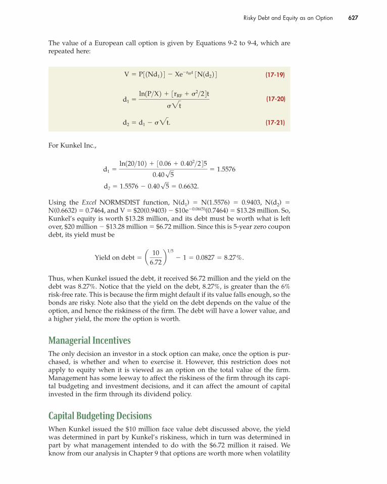
The value of a European call option is given by Equations 9-2 to 9-4, which arerepeated here:
For Kunkel Inc.,
Using the Excel NORMSDIST function, N(d1) � N(1.5576) � 0.9403, N(d2) �
N(0.6632) � 0.7464, and V � $20(0.9403) � $10e�0.06(5)(0.7464) � $13.28 million. So,Kunkel’s equity is worth $13.28 million, and its debt must be worth what is leftover, $20 million � $13.28 million � $6.72 million. Since this is 5-year zero coupondebt, its yield must be
Thus, when Kunkel issued the debt, it received $6.72 million and the yield on thedebt was 8.27%. Notice that the yield on the debt, 8.27%, is greater than the 6%risk-free rate. This is because the firm might default if its value falls enough, so thebonds are risky. Note also that the yield on the debt depends on the value of theoption, and hence the riskiness of the firm. The debt will have a lower value, anda higher yield, the more the option is worth.
Managerial Incentives
The only decision an investor in a stock option can make, once the option is pur-chased, is whether and when to exercise it. However, this restriction does notapply to equity when it is viewed as an option on the total value of the firm.Management has some leeway to affect the riskiness of the firm through its capi-tal budgeting and investment decisions, and it can affect the amount of capitalinvested in the firm through its dividend policy.
Capital Budgeting Decisions
When Kunkel issued the $10 million face value debt discussed above, the yieldwas determined in part by Kunkel’s riskiness, which in turn was determined inpart by what management intended to do with the $6.72 million it raised. Weknow from our analysis in Chapter 9 that options are worth more when volatility
Yield on debt � a 10
6.72b 1>5
� 1 � 0.0827 � 8.27%.
d2 � 1.5576 � 0.40√5 � 0.6632.
d1 �
ln120>10 2 � 30.06 � 0.402>2 450.40√5
� 1.5576
d2 � d1 � �2t.
d1 �
ln1P>X 2 � 3rRF � �2>2 4 t
�2t
V � P 3 1Nd1 2 4 � Xe�rRFt 3N1d2 2 4 (17-19)
(17-20)
(17-21)

628 Chapter 17 Capital Structure Decisions: Extensions
is higher. This means that if Kunkel’s management can find a way to increase itsriskiness without decreasing the total value of the firm, this will increase the valueof the equity while decreasing the value of the debt. Management can do this byselecting risky rather than safe investment projects. Table 17-1 shows the value ofthe equity, debt, and the yield on the debt for a range of possible volatilities. TheTool Kit for this chapter shows the calculations.
Kunkel’s current volatility is 40% so its equity is worth $13.28 million, and itsdebt is worth $6.72 million. However, if, after incurring the debt, managementundertakes projects that increase its riskiness from a volatility of 40% to a volatil-ity of 80%, the value of Kunkel’s equity will increase by $2.53 million to $15.81million, and the value of its debt will decrease by the same amount. This 19%increase in the value of the equity represents a transfer of wealth from the bond-holders to the stockholders. A corresponding transfer of wealth from stockholdersto bondholders would occur if Kunkel undertook projects that were safer thanoriginally planned. Table 17-1 shows that if management undertakes safe projectsand drives the volatility down to 30%, stockholders will lose (and bondholderswill gain) $0.45 million.
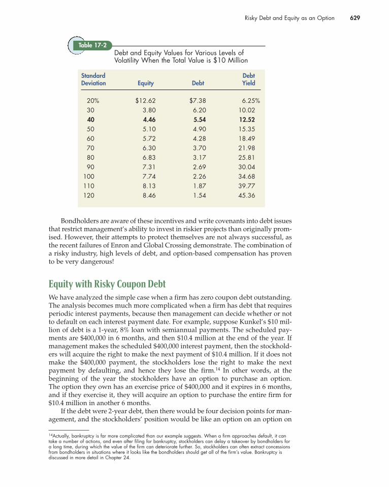
Such a strategy of investing borrowed funds in risky assets is called bait andswitch because the firm obtains the money, promising one investment policy, andthen switches to another policy. The bait and switch problem is more severe when afirm’s value is low relative to its level of debt. When Kunkel’s total value was $20million, doubling its volatility from 40% to 80% increased its equity value by 19%.But if Kunkel had done poorly in recent years and its total value were only $10 mil-lion, then the impact of increasing volatility would be much greater. Table 17-2 showsthat if Kunkel’s total value were only $10 million and if it issued $10 million facevalue of 5-year zero coupon debt, its equity would be worth $4.46 million at a volatil-ity of 40%. Doubling the volatility to 80% would increase the value of the equity to$6.83 million, or by 53%. The incentive for management to “roll the dice” with bor-rowed funds can be enormous, and if management owns lots of stock options, theirpayoff from rolling the dice is even greater than the payoff to the stockholders!
See FM12 Ch 17 ToolKit.xls at the textbook’sWeb site for details.
The Value of Kunkel’s Debt and Equityfor Various Levels of Volatility
Table 17-1
Standard DebtDeviation Equity Debt Yield
20% $12.62 $7.38 6.25%
30 12.83 7.17 6.89
40 13.28 6.72 8.27
50 13.86 6.14 10.25
60 14.51 5.49 12.74
70 15.17 4.83 15.66
80 15.81 4.19 18.99
90 16.41 3.59 22.74
100 16.96 3.04 26.92
110 17.46 2.54 31.56
120 17.90 2.10 36.68
Risky Debt and Equity as an Option 629
Bondholders are aware of these incentives and write covenants into debt issuesthat restrict management’s ability to invest in riskier projects than originally prom-ised. However, their attempts to protect themselves are not always successful, asthe recent failures of Enron and Global Crossing demonstrate. The combination ofa risky industry, high levels of debt, and option-based compensation has provento be very dangerous!
Equity with Risky Coupon Debt
We have analyzed the simple case when a firm has zero coupon debt outstanding.The analysis becomes much more complicated when a firm has debt that requiresperiodic interest payments, because then management can decide whether or notto default on each interest payment date. For example, suppose Kunkel’s $10 mil-lion of debt is a 1-year, 8% loan with semiannual payments. The scheduled pay-ments are $400,000 in 6 months, and then $10.4 million at the end of the year. Ifmanagement makes the scheduled $400,000 interest payment, then the stockhold-ers will acquire the right to make the next payment of $10.4 million. If it does notmake the $400,000 payment, the stockholders lose the right to make the nextpayment by defaulting, and hence they lose the firm.14 In other words, at thebeginning of the year the stockholders have an option to purchase an option.The option they own has an exercise price of $400,000 and it expires in 6 months,and if they exercise it, they will acquire an option to purchase the entire firm for$10.4 million in another 6 months.
If the debt were 2-year debt, then there would be four decision points for man-agement, and the stockholders’ position would be like an option on an option on
14Actually, bankruptcy is far more complicated than our example suggests. When a firm approaches default, it cantake a number of actions, and even after filing for bankruptcy, stockholders can delay a takeover by bondholders fora long time, during which the value of the firm can deteriorate further. So, stockholders can often extract concessionsfrom bondholders in situations where it looks like the bondholders should get all of the firm’s value. Bankruptcy is discussed in more detail in Chapter 24.
Debt and Equity Values for Various Levels ofVolatility When the Total Value is $10 Million
Table 17-2
Standard DebtDeviation Equity Debt Yield
20% $12.62 $7.38 6.25%
30 3.80 6.20 10.02
40 4.46 5.54 12.52
50 5.10 4.90 15.35
60 5.72 4.28 18.49
70 6.30 3.70 21.98
80 6.83 3.17 25.81
90 7.31 2.69 30.04
100 7.74 2.26 34.68
110 8.13 1.87 39.77
120 8.46 1.54 45.36
630 Chapter 17 Capital Structure Decisions: Extensions
an option on an option! These types of options are called compound options, andthe techniques to value them are beyond the scope of this book. However, theincentives discussed above for the case when the firm has risky zero coupon debtstill apply when the firm has to make periodic interest payments.15
15For more on viewing equity as an option, see D. Galai and R. Masulis, “The Option Pricing Model and the RiskFactor of Stock,” Journal of Financial Economics, 1976, pp. 53–81. For a discussion on compound options, seeRobert Geske, “The Valuation of Corporate Liabilities as Compound Options,” Journal of Financial and QuantitativeAnalysis, June 1984, pp. 541–552.
17.6 Capital Structure Theory: Our View
The great contribution of the capital structure models developed by MM, Miller,and their followers is that these models identified the specific benefits and costsof using debt—the tax benefits, financial distress costs, and so on. Prior to MM, nocapital structure theory existed, so we had no systematic way of analyzing theeffects of debt financing.
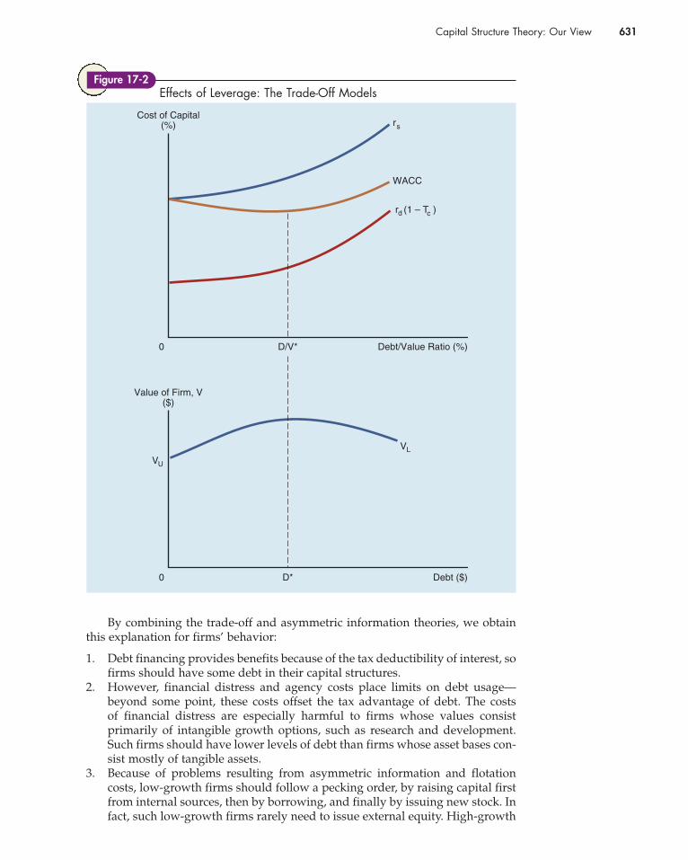
The trade-off model we discussed in Chapter 16 is summarized graphically inFigure 17-2. The top graph shows the relationships between the debt ratio and thecost of debt, the cost of equity, and the WACC. Both rs and rd(1 � Tc) rise steadilywith increases in leverage, but the rate of increase accelerates at higher debt lev-els, reflecting agency costs and the increased probability of financial distress. TheWACC first declines, then hits a minimum at D/V*, and then begins to rise. Notethat the value of D in D/V* in the upper graph is D*, the level of debt in the lowergraph that maximizes the firm’s value. Thus, a firm’s WACC is minimized and itsvalue is maximized at the same capital structure. Note also that the general shapesof the curves apply regardless of whether we are using the modified MM with cor-porate taxes model, the Miller model, or a variant of these models.
Unfortunately, it is impossible to quantify accurately the costs and benefits ofdebt financing, so it is impossible to pinpoint D/V*, the capital structure that maxi-mizes a firm’s value. Most experts believe such a structure exists for every firm, butthat it changes over time as firms’ operations and investors’ preferences change.Most experts also believe that, as shown in Figure 17-2, the relationship betweenvalue and leverage is relatively flat over a fairly broad range, so large deviations fromthe optimal capital structure can occur without materially affecting the stock price.
Now consider signaling theory, which we discussed in Chapter 16. Because ofasymmetric information, investors know less about a firm’s prospects than itsmanagers know. Further, managers try to maximize value for current stockhold-ers, not new ones. Therefore, if the firm has excellent prospects, management willnot want to issue new shares, but if things look bleak, then a new stock offeringwould benefit current stockholders. Consequently, investors take a stock offeringto be a signal of bad news, so stock prices tend to decline when new issues areannounced. As a result, new equity financings are relatively expensive. The neteffect of signaling is to motivate firms to maintain a reserve borrowing capacitydesigned to permit future investment opportunities to be financed by debt ifinternal funds are not available.
Discuss how equity can be viewed as an option. Who has the option and what decision can they make?
Why would management want to increase the riskiness of the firm? Why would this make bondholdersunhappy?
What can bondholders do to limit management’s ability to bait and switch?
SELF-TEST
Capital Structure Theory: Our View 631
By combining the trade-off and asymmetric information theories, we obtainthis explanation for firms’ behavior:
1. Debt financing provides benefits because of the tax deductibility of interest, sofirms should have some debt in their capital structures.
2. However, financial distress and agency costs place limits on debt usage—beyond some point, these costs offset the tax advantage of debt. The costs of financial distress are especially harmful to firms whose values consistprimarily of intangible growth options, such as research and development.Such firms should have lower levels of debt than firms whose asset bases con-sist mostly of tangible assets.
3. Because of problems resulting from asymmetric information and flotationcosts, low-growth firms should follow a pecking order, by raising capital firstfrom internal sources, then by borrowing, and finally by issuing new stock. Infact, such low-growth firms rarely need to issue external equity. High-growth
Debt ($)D*0
VU
VL
Value of Firm, V($)
Debt/Value Ratio (%)D/V*0
r (1 – T )d
Cost of Capital(%)
c
WACC
rs
Effects of Leverage: The Trade-Off ModelsFigure 17-2
632 Chapter 17 Capital Structure Decisions: Extensions
firms whose growth occurs primarily through increases in tangible assetsshould follow the same pecking order, but usually they will need to issue newstock as well as debt. High-growth firms whose values consist primarily ofintangible growth options may run out of internally generated cash, but theyshould emphasize stock rather than debt due to the severe problems thatfinancial distress imposes on such firms.
4. Finally, because of asymmetric information, firms should maintain a reserveof borrowing capacity in order to be able to take advantage of good invest-ment opportunities without having to issue stock at low prices, and thisreserve will cause the actual debt ratio to be lower than that suggested by thetrade-off models.
There is some evidence that managers do attempt to behave in ways that areconsistent with this view of capital structure. In a survey of CFOs, about two-thirdsof the CFOs said that they follow a “hierarchy in which the most advantageoussources of funds are exhausted before other sources are used.” The hierarchy usu-ally followed the pecking order of first internally generated cash flow, then debt,and finally external equity, which is consistent with the predicted behavior of mostlow-growth firms. But there were occasions in which external equity was the firstsource of financing, which would be consistent with the theory for either high-growth firms or firms whose agency and financial distress costs have exceeded thebenefit of the tax savings.16
16For more on capital budgeting issues, see Ravindra R. Kamath, “Long-Term Financing Decisions: Views andPractices of Financial Managers of NYSE Firms,” Financial Review, May 1997, pp. 350–356; Claire E. Crutchleyand Robert S. Hansen, “A Test of the Agency Theory of Managerial Ownership, Corporate Leverage, and CorporateDividends,” Financial Management, Winter 1989, pp. 36–46; Michael T. Dugan and Keith A. Shriver, “An EmpiricalComparison of Alternative Methods for Estimating the Degree of Operating Leverage,” Financial Review, May 1992,pp. 309–321; Dilip K. Ghosh, “Optimum Capital Structure Redefined,” Financial Review, August 1992, pp.411–429; William A. Kelly, Jr., and James A. Miles, “Capital Structure Theory and the Fisher Effect,” FinancialReview, February 1989, pp. 53–73; J. Michael Pinegar and Lisa Wilbricht, “What Managers Think of CapitalStructure Theory: A Survey,” Financial Management, Winter 1989, pp. 82–91; Frederick C. Scherr, “A MultiperiodMean-Variance Model of Optimal Capital Structure,” Financial Review, February 1987, pp. 1–31.
Summarize the trade-off and signaling theories of capital structure.
Are the trade-off and signaling theories mutually exclusive; that is, might both be correct?
Does capital structure theory provide managers with a model that can be used to set a precise optimalcapital structure?
SELF-TEST
Summary
In this chapter, we discussed a variety of topics related to capital structuredecisions. The key concepts covered are listed below:
• In 1958, Franco Modigliani and Merton Miller (MM) proved, under arestrictive set of assumptions including zero taxes, that capital structure isirrelevant; that is, according to the original MM article, a firm’s value is notaffected by its financing mix.
• MM later added corporate taxes to their model and reached the conclusionthat capital structure does matter. Indeed, their model led to the conclusionthat firms should use 100% debt financing.
• MM’s model with corporate taxes demonstrated that the primary benefit ofdebt stems from the tax deductibility of interest payments.

Questions 633
• Later, Miller extended the theory to include personal taxes. The introductionof personal taxes reduces, but does not eliminate, the benefits of debt financ-ing. Thus, the Miller model also leads to 100% debt financing.
• The introduction of growth changes the MM and Hamada results for the lev-ered cost of equity and the levered beta.
• If the firm is growing at a constant rate, the debt tax shield is discounted atrsU, and debt remains a constant proportion of the capital structure, then
and
• When debt is risky, management may choose to default on it. If the debt is zerocoupon debt, then this makes equity like an option on the value of the firm witha strike price equal to the face value of the debt. If the debt has periodic interestpayments, then the equity is like an option on an option, or a compound option.
• When a firm has risky debt and equity is like an option, management has anincentive to increase the firm’s risk in order to increase the equity value at theexpense of the debt value. This is called bait and switch.
Questions
Define each of the following terms:a. MM Proposition I without taxes; with corporate taxesb. MM Proposition II without taxes; with corporate taxesc. Miller modeld. Financial distress costse. Agency costsf. Trade-off modelg. Value of debt tax shieldh. Equity as an option
What term refers to the uncertainty inherent in projections of future ROIC?
Firms with relatively high nonfinancial fixed costs are said to have a high degreeof what?
“One type of leverage affects both EBIT and EPS. The other type affects only EPS.”Explain this statement.
Why is the following statement true? “Other things being the same, firms with rel-atively stable sales are able to carry relatively high debt ratios.”
Why do public utility companies usually have capital structures that are differentfrom those of retail firms?
Why is EBIT generally considered to be independent of financial leverage? Whymight EBIT actually be influenced by financial leverage at high debt levels?
b � bU � 1bU � bD 2DS .
rsL � rsU � 1rsU � rd 2DS
(17-1)
(17-5)
(17-6)
(17-7)
(17-2)
(17-3)
(17-4)
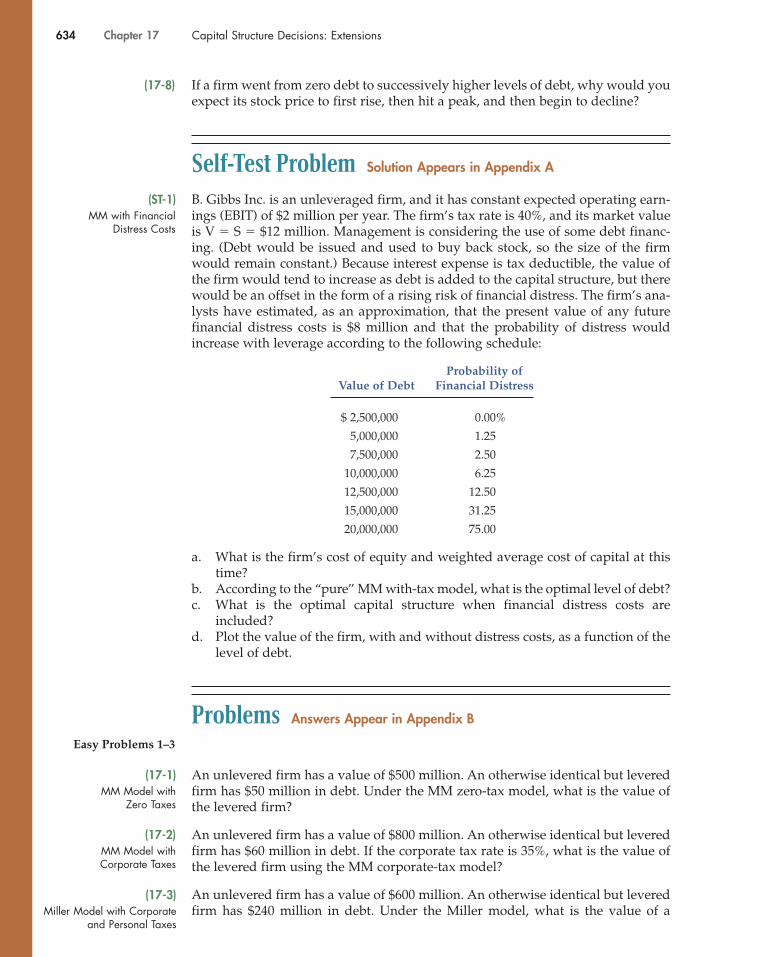
634 Chapter 17 Capital Structure Decisions: Extensions
If a firm went from zero debt to successively higher levels of debt, why would youexpect its stock price to first rise, then hit a peak, and then begin to decline?
Self-Test Problem Solution Appears in Appendix A
B. Gibbs Inc. is an unleveraged firm, and it has constant expected operating earn-ings (EBIT) of $2 million per year. The firm’s tax rate is 40%, and its market valueis V � S � $12 million. Management is considering the use of some debt financ-ing. (Debt would be issued and used to buy back stock, so the size of the firmwould remain constant.) Because interest expense is tax deductible, the value ofthe firm would tend to increase as debt is added to the capital structure, but therewould be an offset in the form of a rising risk of financial distress. The firm’s ana-lysts have estimated, as an approximation, that the present value of any futurefinancial distress costs is $8 million and that the probability of distress wouldincrease with leverage according to the following schedule:
(17-8)
MM with FinancialDistress Costs
(ST-1)
Probability ofValue of Debt Financial Distress
$ 2,500,000 0.00%
5,000,000 1.25
7,500,000 2.50
10,000,000 6.25
12,500,000 12.50
15,000,000 31.25
20,000,000 75.00
Easy Problems 1–3
MM Model withZero Taxes
(17-1)
MM Model withCorporate Taxes
(17-2)
Miller Model with Corporateand Personal Taxes
(17-3)
a. What is the firm’s cost of equity and weighted average cost of capital at thistime?
b. According to the “pure” MM with-tax model, what is the optimal level of debt?c. What is the optimal capital structure when financial distress costs are
included?d. Plot the value of the firm, with and without distress costs, as a function of the
level of debt.
Problems Answers Appear in Appendix B
An unlevered firm has a value of $500 million. An otherwise identical but leveredfirm has $50 million in debt. Under the MM zero-tax model, what is the value ofthe levered firm?
An unlevered firm has a value of $800 million. An otherwise identical but leveredfirm has $60 million in debt. If the corporate tax rate is 35%, what is the value ofthe levered firm using the MM corporate-tax model?
An unlevered firm has a value of $600 million. An otherwise identical but leveredfirm has $240 million in debt. Under the Miller model, what is the value of a
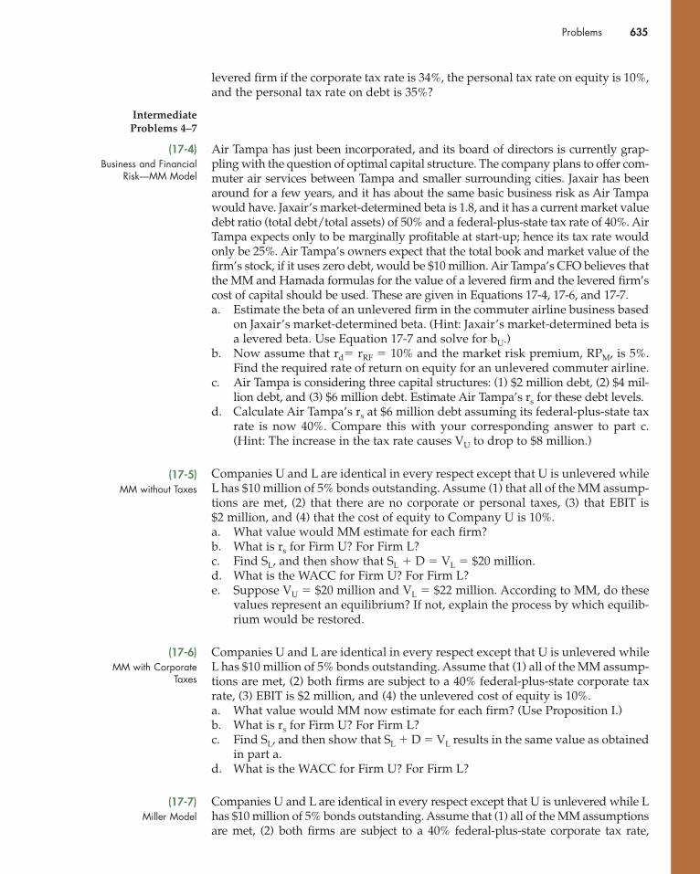
Problems 635
levered firm if the corporate tax rate is 34%, the personal tax rate on equity is 10%,and the personal tax rate on debt is 35%?
Air Tampa has just been incorporated, and its board of directors is currently grap-pling with the question of optimal capital structure. The company plans to offer com-muter air services between Tampa and smaller surrounding cities. Jaxair has beenaround for a few years, and it has about the same basic business risk as Air Tampawould have. Jaxair’s market-determined beta is 1.8, and it has a current market valuedebt ratio (total debt/total assets) of 50% and a federal-plus-state tax rate of 40%. AirTampa expects only to be marginally profitable at start-up; hence its tax rate wouldonly be 25%. Air Tampa’s owners expect that the total book and market value of thefirm’s stock, if it uses zero debt, would be $10 million. Air Tampa’s CFO believes thatthe MM and Hamada formulas for the value of a levered firm and the levered firm’scost of capital should be used. These are given in Equations 17-4, 17-6, and 17-7.a. Estimate the beta of an unlevered firm in the commuter airline business based
on Jaxair’s market-determined beta. (Hint: Jaxair’s market-determined beta isa levered beta. Use Equation 17-7 and solve for bU.)
b. Now assume that rd� rRF � 10% and the market risk premium, RPM, is 5%.Find the required rate of return on equity for an unlevered commuter airline.
c. Air Tampa is considering three capital structures: (1) $2 million debt, (2) $4 mil-lion debt, and (3) $6 million debt. Estimate Air Tampa’s rs for these debt levels.
d. Calculate Air Tampa’s rs at $6 million debt assuming its federal-plus-state taxrate is now 40%. Compare this with your corresponding answer to part c.(Hint: The increase in the tax rate causes VU to drop to $8 million.)
Companies U and L are identical in every respect except that U is unlevered whileL has $10 million of 5% bonds outstanding. Assume (1) that all of the MM assump-tions are met, (2) that there are no corporate or personal taxes, (3) that EBIT is$2 million, and (4) that the cost of equity to Company U is 10%.a. What value would MM estimate for each firm?b. What is rs for Firm U? For Firm L?c. Find SL, and then show that SL � D � VL � $20 million.d. What is the WACC for Firm U? For Firm L?e. Suppose VU � $20 million and VL � $22 million. According to MM, do these
values represent an equilibrium? If not, explain the process by which equilib-rium would be restored.
Companies U and L are identical in every respect except that U is unlevered whileL has $10 million of 5% bonds outstanding. Assume that (1) all of the MM assump-tions are met, (2) both firms are subject to a 40% federal-plus-state corporate taxrate, (3) EBIT is $2 million, and (4) the unlevered cost of equity is 10%.a. What value would MM now estimate for each firm? (Use Proposition I.)b. What is rs for Firm U? For Firm L?c. Find SL, and then show that SL � D � VL results in the same value as obtained
in part a.d. What is the WACC for Firm U? For Firm L?
Companies U and L are identical in every respect except that U is unlevered while Lhas $10 million of 5% bonds outstanding. Assume that (1) all of the MM assumptionsare met, (2) both firms are subject to a 40% federal-plus-state corporate tax rate,
Intermediate Problems 4–7
Business and FinancialRisk—MM Model
(17-4)
MM with CorporateTaxes
(17-6)
MM without Taxes
(17-5)
Miller Model
(17-7)

636 Chapter 17 Capital Structure Decisions: Extensions
(3) EBIT is $2 million, (4) investors in both firms face a tax rate of Td � 28% on debtincome and Ts � 20%, on average, on stock income, and (5) the appropriate requiredpre-personal-tax rate rsU is 10%.a. What is the value of the unlevered firm, VU? (Note that VU is now reduced by
the personal tax on stock income; hence VU � $12 million as in Problem 17-6.)b. What is the value of VL?c. What is the gain from leverage in this situation? Compare this with the gain
from leverage in Problem 17-6.d. Set Tc � Ts � Td � 0. What is the value of the levered firm? The gain from
leverage?e. Now suppose Ts � Td � 0, Tc� 40%. What are the value of the levered firm
and the gain from leverage?f. Assume that Td � 28%, Ts � 28%, and Tc � 40%. Now what are the value of
the levered firm and the gain from leverage?
Schwarzentraub Industries’ expected free cash flow for the year is $500,000; in thefuture free cash flow is expected to grow at a rate of 9%. The company currentlyhas no debt, and its cost of equity is 13%. Its tax rate is 40%. (Hint: Use Equations17-16 and 17-17.)a. Find VU.b. Find VL and rsL if Schwarzentraub uses $5 million in debt with a cost of 7%.
Use the extension to the MM model that allows for growth.c. Based on VU from part a, find VLand rsL using the MM model (with taxes) if
Schwarzentraub uses $5 million in 7% debt.d. Explain the difference between the answers to parts b and c.
International Associates (IA) is just about to commence operations as an interna-tional trading company. The firm will have book assets of $10 million, and itexpects to earn a 16% return on these assets before taxes. However, because of cer-tain tax arrangements with foreign governments, IA will not pay any taxes; thatis, its tax rate will be zero. Management is trying to decide how to raise therequired $10 million. It is known that the capitalization rate for an all-equity firmin this business is 11%; that is, rU � 11%. Further, IA can borrow at a rate rd � 6%.Assume that the MM assumptions apply.a. According to MM, what will be the value of IA if it uses no debt? If it uses $6
million of 6% debt?b. What are the values of the WACC and rs at debt levels of D � $0, D � $6 mil-
lion, and D � $10 million? What effect does leverage have on firm value? Why?c. Assume the initial facts of the problem (rd � 6%, EBIT � $1.6 million, rsU �
11%), but now assume that a 40% federal-plus-state corporate tax rate exists.Find the new market values for IA with zero debt and with $6 million of debt,using the MM formulas.
d. What are the values of the WACC and rs at debt levels of D � $0, D �
$6 million, and D � $10 million, assuming a 40% corporate tax rate? Plot therelationships between the value of the firm and the debt ratio, and betweencapital costs and the debt ratio.
e. What is the maximum dollar amount of debt financing that can be used? Whatis the value of the firm at this debt level? What is the cost of this debt?
ChallengingProblems 8–10
MM Extensionwith Growth
(17-8)
MM with andwithout Taxes
(17-9)

Mini Case 637
f. How would each of the following factors tend to change the values youplotted in your graph?(1) The interest rate on debt increases as the debt ratio rises.(2) At higher levels of debt, the probability of financial distress rises.
A. Fethe Inc. is a custom manufacturer of guitars, mandolins, and other stringedinstruments located near Knoxville, Tennessee. Fethe’s current value of opera-tions, which is also its value of debt plus equity, is estimated to be $5 million.Fethe has $2 million face-value zero coupon debt that is due in 2 years. The risk-free rate is 6%, and the standard deviation of returns for companies similar toFethe is 50%. Fethe’s owners view their equity investment as an option and wouldlike to know the value of their investment.a. Using the Black-Scholes Option Pricing Model, how much is Fethe’s equity
worth?b. How much is the debt worth today? What is its yield?c. How would the equity value and the yield on the debt change if Fethe’s man-
agers were able to use risk management techniques to reduce its volatility to30%? Can you explain this?
Spreadsheet Problem
Start with the partial model in the file FM12 Ch 17 P11 Build a Model.xls at thetextbook’s Web site. Rework Problem 17-10 using a spreadsheet model. Aftercompleting the problem as it appears, answer the following related questions.a. Graph the cost of debt versus the face value of debt for values of the face value
from $0.5 to $8 million.b. Graph the values of debt and equity for volatilities from 0.10 to 0.90 when the
face value of the debt is $2 million.c. Repeat part b, but instead using a face value of debt of $5 million. What can
you say about the difference between the graphs in part b and part c?
Cyberproblem
Please go to the textbook’s Web site to access any Cyberproblems.
Equity Viewed asan Option
(17-10)
Build a Model: EquityViewed as an Option
(17-11)
See FM12 Ch 17 P11Build a Model.xls fordetails.
Mini Case
David Lyons, CEO of Lyons Solar Technologies, is concerned about his firm’s levelof debt financing. The company uses short-term debt to finance its temporary work-ing capital needs, but it does not use any permanent (long-term) debt. Other solartechnology companies average about 30% debt, and Mr. Lyons wonders why theyuse so much more debt and how it affects stock prices. To gain some insights intothe matter, he poses the following questions to you, his recently hired assistant:a. BusinessWeek recently ran an article on companies’ debt policies, and the
names Modigliani and Miller (MM) were mentioned several times as leading
638 Chapter 17 Capital Structure Decisions: Extensions
researchers on the theory of capital structure. Briefly, who are MM, and whatassumptions are embedded in the MM and Miller models?
b. Assume that Firms U and L are in the same risk class, and that both have EBIT � $500,000. Firm U uses no debt financing, and its cost of equity is rsU �
14%. Firm L has $1 million of debt outstanding at a cost of rd � 8%. There areno taxes. Assume that the MM assumptions hold, and then:(1) Find V, S, rs, and WACC for Firms U and L.(2) Graph (a) the relationships between capital costs and leverage as meas-
ured by D/V, and (b) the relationship between value and D.c. Using the data given in part b, but now assuming that Firms L and U are both
subject to a 40% corporate tax rate, repeat the analysis called for in b-(1) andb-(2) under the MM with-tax model.
d. Now suppose investors are subject to the following tax rates: Td � 30% and Ts � 12%.(1) What is the gain from leverage according to the Miller model?(2) How does this gain compare with the gain in the MM model with
corporate taxes?(3) What does the Miller model imply about the effect of corporate debt on
the value of the firm; that is, how do personal taxes affect the situation?e. What capital structure policy recommendations do the three theories (MM
without taxes, MM with corporate taxes, and Miller) suggest to financial man-agers? Empirically, do firms appear to follow any one of these guidelines?
f. How is the analysis in part c different if Firms U and L are growing? Assumethat both firms are growing at a rate of 7% and that the investment in net oper-ating assets required to support this growth is 10% of EBIT.
g. What if L’s debt is risky? For the purpose of this example, assume that the valueof L’s operations is $4 million—which is the value of its debt plus equity.Assume also that its debt consists of 1-year zero coupon bonds with a face valueof $2 million. Finally, assume that L’s volatility is 0.60 (� � 0.60) and that therisk-free rate is 6%.
h. What is the value of L’s stock for volatilities between 0.20 and 0.95? Whatincentives might the manager of L have if she understands this relationship?What might debtholders do in response?
The following cases from Textchoice, ThomsonLearning’s online library, cover many of the conceptsdiscussed in this chapter and are available athttp://www.textchoice2.com.
Klein-Brigham Series:Case 7, “Seattle Steel Products,” Case 9, “KleenKar, Inc.,” Case 10, “Aspeon Sparkling Water,”Case 43, “Mountain Springs,” Case 57, “GretaCosmetics,” Case 74, “The Western Company,”Case 83, “Armstrong Production Company,” and
Case 99, “Moore Plumbing Supply Company,”focus on capital structure theory. Case 8, “JohnsonWindow Company,” and Case 56, “Isle MarineBoat Company,” cover operating and financialleverage.
Brigham-Buzzard Series:Case 8, “Powerline Network Corporation,” coversoperating leverage, financial leverage, and theoptimal capital structure.
Selected Additional Cases
Related Documents