Chapter 16 Predator-Prey Coevolution

Chapter 16

Predator-Prey Coevolution

Linda R. Van Thiel

Department of Biological Sciences Wayne State University Detroit, Michigan 48202

(313) 577-2776

Linda is the laboratory coordinator for the introductory biology course for non-majors and the two-semester freshman biology sequence for majors at Wayne State University. Linda received her B.S. in Biology from Northern Illinois University in 1973 and her M.S. in Physiology from Michigan State University in 1977. She has been in her present position since 1977. In addition to writing organizational materials and selected handouts for the three courses she coordinates, Linda has written a laboratory manual entitled Laboratory Exercises in Biology: From Chemistry to Sex, now in its third edition. She has also prepared pedagogical materials for the biology text authored by Peter Raven and George Johnson, published by Mosby Year Book; these materials include the extensive Instructor’s Resource Manual that accompanies the text. Her research interests include introductory laboratory instruction and the development of fool-proof, inexpensive laboratory exercises.

© 1994 Linda R. Van Thiel 293

Reprinted from: Van Thiel, L. R. 1994. Predator-prey coevolution. Pages 293-318, in Tested studies for laboratory teaching, Volume 15 (C. A. Goldman, Editor). Proceedings of the 15th Workshop/Conference of the Association for Biology Laboratory Education (ABLE), 390 pages.

- Copyright policy: http://www.zoo.utoronto.ca/able/volumes/copyright.htm

Although the laboratory exercises in ABLE proceedings volumes have been tested and due consideration has been given to safety, individuals performing these exercises must assume all responsibility for risk. The Association for Biology Laboratory Education (ABLE) disclaims any liability with regards to safety in connection with the use of the exercises in its proceedings volumes.

Association for Biology Laboratory Education (ABLE) ~ http://www.zoo.utoronto.ca/able

294 Predator-Prey Coevolution

Contents Introduction....................................................................................................................294 Materials ........................................................................................................................295 Notes for the Instructor ..................................................................................................296 Additional Directions.....................................................................................................296 Computer Instructions....................................................................................................296 Variations on the Theme................................................................................................297 Student Outline ..............................................................................................................298 Introduction....................................................................................................................298 Procedures......................................................................................................................301 Predator Calculations.....................................................................................................303 Prey Calculations ...........................................................................................................304 Student Questions ..........................................................................................................305 Appendix A: Tables for Data Collection .......................................................................306 Appendix B: Further Reading........................................................................................307 Appendix C: Predator-Prey Worksheet Formulae .........................................................308 Appendix D: Predator-Prey New Predator Number Formulae......................................309 Appendix E: Macintosh Excel Spreadsheet Tables .......................................................310 Appendix F: Sample Data Tables and Graphs...............................................................310 Introduction This laboratory exercise is distinctly different from the multitude of exercises that examine the fluctuations of prey and predator populations over many generations, that is, the typical rabbit-fox or deer-wolf situations. This exercise mandates that the total populations of prey and predator do not change over time. What may change is the number of individuals of each phenotype morph for prey and predators through interactive selective forces. If each predator morph captures approximately the same number of each prey morph, the numbers of each predator and prey morph in successive generations will not change significantly. When one predator morph captures significantly more or fewer prey, the numbers of each of the predator morphs change in the next generation. Similarly, if one prey morph is captured to a greater or lesser extent than the others, the number of each prey morph will change in the next generation. In this respect, therefore, this exercise does truly examine the evolution of a species and co-evolution of two interacting species as the numbers of each predator and prey morph change over successive generations. In addition to examining the selective pressures incurred by the type of predator morph, performing this exercise as described using two habitats examines the additional selective pressures conferred by the habitat. This provides for further discussions relating ecology and evolution. We have successfully presented this laboratory exercise at three different levels: introductory non-majors, introductory majors, and sophomore/junior ecology. The students at the introductory levels are not expected to understand the predator-prey calculations as fully as the ecology students. The amount of time spent on the theoretical background and the predator and prey calculations therefore needs to be adjusted accordingly. The beginning students are also provided with computer-generated data tables and graphs. The more advanced students are expected to construct their own tables and graphs. The optimum number of students foraging at any one time is probably 12, initially 4 of each predator, although we have worked with groups as small as 6 and as large as 15. The size and shape of the habitat area (i.e., lab table) further dictate the optimal number. If the class size is large enough, both habitats should be run simultaneously otherwise there may not be enough time in a 3-

Predator-Prey Coevolution 295

hour lab to introduce the topic, perform the exercise, and discuss the results. The procedures in the Student Outline, though, are written so that the two habitats are run sequentially. In all three classes, we expect the students to write a laboratory report. Again, the prepared tables and graphs ensure that all of the students in the less advanced classes start at the same point. The first time the exercise was performed with the introductory non-majors they were expected to construct their own graphs. Unfortunately, very few of the students had the ability to do this well. Their analysis of the data, therefore, suffered. At this level, I feel that the analysis of the data is the more important concept and thus I constructed a computer spreadsheet to generate the graphs. This spreadsheet also ensures accuracy, substantially reduces the time spent calculating the next generation values, and allows more time for discussing the results. In general, this is an entertaining, easily performed, inexpensive laboratory exercise. Dried beans are most readily obtained at a bulk foods store. Other types of prey can be substituted as well as indicated in the section entitled Variations on the Theme. I strongly recommend that plastic utensils be used the first time around just in case the first time is also the last time. If deemed successful, sturdy silverware is obtained more cheaply at a restaurant supply or warehouse store. When nature and class size allow, this exercise is best performed outside using a section of wide sidewalk and an equally-sized expanse of lawn as the two habitats. One drawback though, is that it is virtually impossible to collect all of the prey at the end of the exercise and one can expect to provide a full complement of prey for each laboratory section. Several problems are possible with this laboratory exercise. For some reason, the students want to return the prey captured in a round and add back the calculated number as well. This is not appropriate! To prevent this, make sure that they give you (the “Supreme Ruler”) their prey immediately after counting them. Collect each morph and then have the students count the number to be added for the next generation from this pool. Occasionally, the person entering data does it improperly by paying poor attention to the predator/row or prey/column distinctions. This often goes unnoticed. Although the evolutionary trends are affected, the exercise is not ruined unless numbers of prey captured are entered in a row in which a predator morph has become extinct. If this occurs on my spreadsheet, the total for that row (the extreme right hand column) will return the phrase “no forks!” (or knives, or spoons) as a warning. Similarly if more prey are reported captured than were initially in the environment, the total for that morph column will report the phrase “too many!” If more prey of all morphs are reported captured than were known to be in the environment, the total number of prey cell will report the phrase “OOPS!” Materials This list assumes a class of 24 students with both habitats running concurrently:

Student collection cups (24) Silverware morph: fork, knife, spoon (24 of each) Dried bean morphs: garbanzo, lentil, lima, pea (2 packages of exactly 500 for each) Extra dried bean morphs: garbanzo, lentil, lima, pea (2 packages of about 500 for each) Prey stockade cups (labeled): garbanzo, lentil, lima, pea (8) Foam mattress pad Calculators (minimum of 2) Computer with printer (optional, but strongly recommended)


Notes for the Instructor Additional Directions When there are multiple sections of a course being run, the first instructor should use the prey in the counted packets of 500 to start the exercise. Use the prey in the uncounted packets to add to the prey morphs that are increasing in the second and third generations. Leave the excess prey for the morphs that are decreasing in the appropriate prey stockade. Use the uncounted prey to replace prey that become physically damaged or those that escape where you cannot reach them (i.e., down a drain, under a cabinet). At the end of each class you must return the total number of each prey to 500. This should be fairly easy to do since you have the total count for each predator for the last round. Add or subtract to make 500 and place these in the appropriate package for 500. Any prey over 500 should be put in the appropriate uncounted packet(s). If for any reason you cannot return the total to 500, leave a note so that the next instructor does not start his/her session blindly with incorrect numbers! With regard to predators, if your class is not evenly divisible by three you may elect to participate as a predator if you are short by only one. Alternately, you may select one or two students whose counts will be doubled. Produce graphs for each generation via the computer if one is available. Reduce, then cut and paste (or tape) two or three graphs per page, and finally photocopy for each student in your class.

Computer Instructions All of the calculations necessary to do this experiment have been entered on a computer spreadsheet available from the author. Both Macintosh and MS-DOS versions are available. The Mac version is written in Excel 4.0. This spreadsheet can also be directly imported into MS-DOS Excel for Windows. The MS-DOS versions available include the earliest version of Lotus 1-2-3 (extension *.wks), version 2 of the same program (extension *.wk1), an early version of Borland’s Quattro (extension *.wkq), and a later version of Borland’s Quattro Pro (extension *.wq!). In general, the near-universal spreadsheet standard is the Lotus 1-2-3 *.wks file. I have found that nearly every spreadsheet, database, or word processing program can import such a file with very little difficulty. Consult the reference manual for the program available to you. The only negative point associated with importing the basic *.wks file is that it is so primitive that the warning phrases described in the fifth paragraph of the Introduction cannot be implemented. I will be glad to send a copy of the spreadsheet file(s) to any one requesting them. Please send a formatted disk or a check for $3.00 US to me and indicate what type of computer system(s) and spreadsheet program(s) you have available. As we have used both Quattro Pro and Macintosh Excel 4.0, I have basic directions for those programs available as well and will send you whichever seems most appropriate. You may need to restructure some of the graphic and printing parameters associated with the spreadsheet files to accommodate your specific computer system and printer. To prevent the inadvertent over-writing of any formulae in the spreadsheet, data can be entered only in the specified area, the brighter or different-colored portion of the screen. The rest of the spreadsheet is protected without a password. The data and calculations for each generation are visible on a single computer screen and are analogous to the tables present in the student's exercise.


Variations on the Theme Substitute other silverware morphs for the common fork, knife, and spoon. These could include the morphs of the large species Argentum megaserverous, specifically the meat fork, serving spoon, and carving knife. Obtaining these morphs, though, is significantly more costly for the Supreme Ruler. One could also enlist the species at the opposite end of the spectrum, Argentum humiliorus, that include the seafood fork, butter knife, and sugar spoon. Interesting data could also be acquired through the use of hybrid morphs like the grapefruit spoon with its serrated projections on its anterior edge. Substitute mutant plasticware for silverware. These forms are nearly identical in physical and behavioral attributes but lack the hard, shiny exoskeleton of the typical Argentum species. They are, therefore, quite brittle and have a much lower survival rate over time than the non-mutants. For this reason each plasticware individual produces significantly greater numbers of progeny in each successive generation than do the typical morphs that reproduce only to replace their own numbers. Plasticware probably most closely follows a Type III survivorship curve, while silverware more closely follows a Type I or Type II curve. The mutant hybrid spork, commonly found in fast food restaurants, would be an especially curious morph to test. It is a mutant with the additional hybrid attributes of the grapefruit spoon. Substitute other prey for the dried beans. One could use the multi-morphed prey, Pasta nonebullientum, that originated in China, but established significantly greater morphological diversity on the Italian peninsula. Cerealis frigidus is a type of prey enjoyed by silverware predators due to their ability to store sugar in very high amounts. This species is amphibious and inhabits both terrestrial and aquatic habitats. While most dry cereal morphs behave similarly on land, when immersed in liquid some remain crunchy and others become soggy, some float and others sink. A most interesting morph, commonly called the rice crispy, elicits a mating call when aquatic and can be identified by its characteristic “snap, crackle, pop.” Provide various colored and textured habitats on which the predators and prey can coevolve. A deep pile shag carpet provides a jungle-like habitat in which the smaller prey can readily hide. The sharper-toothed predators also have a tendency to get caught in the entwined strands. This can also be turned into an outdoor laboratory exercise providing such habitats as a sandbox, a small wading pool, a sidewalk or driveway, and/or a patch of lawn. In the latter example especially, one should provide substantially greater quantities of prey morphs as it will be impossible to collect the strays when the exercise is completed. At least though, the lost prey will be used as a food source by other furry and feathery prey organisms. Finally, one could assign students to physically adapt their predator to better capture one or more prey morphs. Alternately, adapt the prey to better evade capture by one or all predators. Determine whether such adaptation will prescribe to gradualism or punctuated evolutionary trends.


Student Outline

Introduction

Living organisms within a community interact in a variety of ways. The primary relationship between predator and prey is a familiar one. The predator organism finds the prey organism and uses it as a source of nutrition. It is quite obvious that this relationship is beneficial for the predator and deleterious for the prey. Through the process of evolution, a prey population with sufficient species diversity can, over time, change with respect to being preyed upon to increase their survivability. Some of the organisms within the population may display characteristics that decrease their chance of being eaten. These characteristics confer a reproductive advantage, the individuals survive, reproduce, and have a greater number of offspring that exhibit these positive characteristics. Other organisms may display negative characteristics that result in a greater chance of being preyed upon. Their traits will decrease within the population as these organisms fail to reproduce and pass on their traits. Through the process of natural selection these individuals are said to be selected against. Those with positive traits will become more common in future populations. Individuals within a species that have slightly different visible characteristics, or phenotypes, are called morphs. The genetic variation present is not significant enough to qualify the individuals as being different species. The existence of morphs merely reflects the overall genetic diversity within a species. Many forces within nature act upon the predator population that are not directly related to predation but nonetheless affect survival and reproductive fitness. Individuals that are well equipped to escape from predators may succumb to disease while enough of those that are good prey (at least to the predator) may survive to reproduce and pass on their genes. Because these natural forces change from year to year, the characteristics of individuals within a population vary over time. Traits that are reproductively advantageous one year may be deleterious the next. As a result, a great degree of genetic diversity is maintained within a species over time. This diversity enables a species to survive totally unexpected changes in the environment. Contrary to popular opinion, an alteration in the environment does not cause a change in an individual's genes. Rather it affects the entire population by allowing only those with an already different genetic pattern to survive. The peppered moth (Biston betularia) provides one of the best known examples of morph success in varying environments. Prior to the industrial revolution in Britain, the peppered moth existed primarily in its light-colored morph. These individuals were nearly invisible on the light lichen-covered trees on which they rested. A dark morph of the peppered moth existed, but individuals were rare as they were easy targets for birds. Surprisingly, the gene for dark coloration is dominant over the light gene. As industry increased, the tree trunks became darkened and the lichens were killed by the pollutants. The light-colored moths became the easy prey against the darker background while the dark individuals became difficult to spot. As a result fewer of the light morph and more of the dark morph survived to reproduce. The population of pepper moths in the industrialized areas shifted to the dark variety. In non-polluted areas though, the light-colored moth remained the predominant morph. The peppered moth, a prey species, therefore exhibits two morphs each with a greater or lesser ability to escape predation relative to the environment. Similarly, predators have morphs with different abilities to capture prey. A complex interaction exists between predator and prey species, and between each of them and its environment that enables each to survive, reproduce, and evolve. The evolution of each species is so closely connected with the evolution of the other that the two are said to coevolve with respect to one another. It is the interactive selection associated with this process that will be examined in this laboratory exercise. A simple series of encounters will illustrate how the physical and behavioral traits of different morphs of prey affect the survival and reproduction of each predator morph and vice versa.


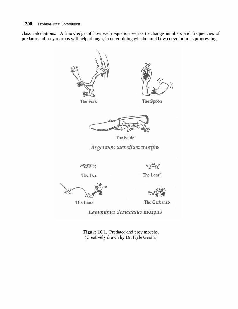
The predator in this exercise is the steely Argentum utensilum, commonly known as silverware (Figure 16.1). This ferocious species exhibits numerous morphs, the most common of which are the dinner knife, dinner fork, and teaspoon. Although the business end of each morph appears quite different, all possess a streamlined body that enables them to streak across the surface of their environs. All three morphs possess a mirror-like coat that reflects images of the habitat, confuses their prey and blinds them in bright sunlight. The favorite prey of all silverware is the meek, unassuming dried bean, Leguminus desicantus. In its mature form, the dried bean is protected by a hard coat that resists the stabbing of the fork predator morph and the smashing of the knife and spoon morphs. The bean also exhibits several morphs including the small, round pea; the large, nearly flat lima; the small, ovoid lentil; and the obese, rotund garbanzo. The peas and garbanzos are the more active of the four morphs and nimbly roll away from their captors. The dried bean is widespread, but proliferates in two primary habitats: the hard, flat, homogenous tabletop tundra and the soft, pliable hills and valleys of the foam mini-mountains. Every student in the class assumes the identity of a silverware predator and forages for the elusive dried bean prey. Each series of foraging between predator and prey corresponds to one reproductive cycle. At the end of each series, the number of each prey and predator morph will be adjusted according to calculations performed by the laboratory instructor (a.k.a. the Supreme Ruler). The bean morphs that succeed at evading capture will have their numbers increased as they produce a greater number of offspring. Those that are readily preyed upon will decrease in number in the next round as an ingested bean cannot reproduce. The frequency of each bean morph will, therefore, change in subsequent foraging series. Similarly, the frequency of each predator morph will change according to its success, or lack thereof. A silverware that captures many beans can produce a greater number of offspring; one that captures few or none cannot reproduce. The frequency of the successful predator will increase while the frequency of the poor predator will decrease. A highly unsuccessful predator may, in time, totally disappear from a given habitat. The total number of predators and prey remains constant through all generations, only the frequency of each morph changes. Therefore, the predator and prey populations evolve as the frequencies of the morphs change. Since the frequency of predator morph is dependent on the prey morph, the two are coevolving over time. The way in which this coevolution progresses may also be affected by the habitat in which the foraging takes place. The final analysis of this exercise will include comments about the coevolution in each habitat as well as a comparison between the two habitats. The initial assignment of student to predator is random. If a predator morph frequency decreases, the Supreme Ruler decides which student predator lives or dies. Since the total number of predators remains constant, the dead predator has the opportunity to be born again as a potentially more successful predator. As in all natural communities, there are several rules that control the foraging for prey by predators. These include, but are not limited to, those listed below:

1. Forage with silverware only — Argentum predators do not have hands! 2. Bean morphs can be captured only one at a time. Mass preying is not allowed. 3. Captured beans must be placed in the forager's collecting cup before foraging can continue. 4. Any bean that escapes the cup must be returned to the habitat. 5. A predator cannot physically alter its shape. 6. Predators cannot interfere with other predators. 7. Predators cannot steal the prey of others as long as the prey is in physical contact with the predator or

his/her collecting cup. 8. The Supreme Ruler will pick up and return any prey that escape the habitat. The calculations for the predator and prey frequency adjustments are presented after the laboratory procedures. Students are not required to memorize these equations nor are they expected to perform the


class calculations. A knowledge of how each equation serves to change numbers and frequencies of predator and prey morphs will help, though, in determining whether and how coevolution is progressing.

Figure 16.1. Predator and prey morphs. (Creatively drawn by Dr. Kyle Geran.)


Procedures 1. Randomly scatter 500 dried beans of each prey morph across the tabletop tundra habitat. Pick

up any that fall into the sink canyon or on the floor abyss. 2. The Supreme Ruler will divide the class into three equal groups and randomly assign each

group to be either a knife, fork, or spoon predator morph. He/she will distribute the silverware appropriately.

3. Enter the numbers of each predator and prey morph on the top and along the left side of the Tundra First Generation results table (Table 16.1).

4. The Supreme Ruler will signal the onset of the first round of foraging and allow it to continue for 3 minutes. Predators must follow the foraging rules previously stated!

5. After the first round is completed, each predator will count the number of each prey morph it captured and calculate the total number of prey. Enter this data in the Tundra First Generation results table and report it to the Supreme Ruler as well.

6. Place the captured beans in the appropriate prey stockades. Do not return the prey to the habitat.

7. Data from the entire class will be tabulated by the Supreme Ruler and shared with all students. He/she will use this data to calculate the numbers of predators and prey for the next round of foraging. Record the results of the Supreme Ruler's calculations at the bottom of the Tundra First Generation results table (Table 16.1).

8. Adjust the student predator identities as instructed by the Supreme Ruler. Using prey from the stockade, add the appropriate number of each bean morph to the habitat as instructed by the Supreme Ruler. Enter the new numbers of predators and prey at the top and along the left side of the Tundra Second Generation results table (see Appendix A).

9. Begin the second 3-minute round of tundra foraging. Repeat steps 3 to 8 compiling results for the second generation.

10. After the Supreme Ruler completes his/her calculations, enter the results in the chart at the bottom of the Tundra Second Generation results table (see Appendix A).

11. Begin the third 3-minute round of foraging on the tabletop tundra. Repeat steps 3 to 7 compiling results for the third generation. Do not add prey back into the tabletop habitat.

12. After the Supreme Ruler completes his/her calculations, enter the results in the chart at the bottom of the Tundra Third Generation results table (see Appendix A).

13. Calculate the number of prey in the tabletop tundra habitat. If there are more than 500 individuals of a prey morph, subtract the excess and transfer all individuals of that morph to the foam mini-mountains habitat. If there are fewer than 500 individuals of a morph, transfer these to the mountains and add more individuals from the appropriate prey stockade to bring the total to 500.

14. Students should return to their initial predator identities as determined in step 2. Enter the numbers of each predator and prey morph on the top and along the left side of the Foam Mini-Mountains First Generation results table (see Appendix A).


15. Begin the first 3-minute round of mountain foraging. Repeat steps 3 to 8 compiling results for the first foam mini-mountains generation.

Table 16.1. Tundra first generation results. Tabletop Tundra

1st generation

Prey

Number of individuals at start Garbanzo Lentil Lima Pea Total

Predators Number of individuals caught Your

identity Your results →

Number of individuals

Morph Garbanzo Lentil Lima Pea Total of all prey

Fork

Knife

Spoon

Total of all predators

*

* Total number of all prey caught by all predators Next generation prey Garbanzo Lentil Lima Pea Total

Add to habitat New total number

Next generation predator Fork Knife Spoon Total New numbers

16. After the Supreme Ruler completes his/her calculations, enter the results in the chart at the

bottom of the Foam Mini-Mountains First Generation results table (see Appendix A).

17. Begin the second 3-minute round of mountain foraging. Repeat steps 3 to 8 compiling results for the second generation.

18. After the Supreme Ruler completes his/her calculations, enter the results in the chart at the bottom of the Foam Mini-Mountains Second Generation results table (see Appendix A).

19. Begin the third 3-minute round of foraging on the mountains. Repeat steps 3 to 7 compiling results for the third generation. Do not add prey back into the foam mini-mountains habitat. Return all captured prey to the appropriate stockade.

20. After the Supreme Ruler completes his/her calculations, enter the results in the chart at the bottom of the Foam Mini-Mountains Third Generation results table (see Appendix A).


21. Students should collect all prey and return them to the appropriate morph stockade. Work collectively to re-establish a package of 500 individuals for each prey morph. Students should also relinquish their predator and return the silverware to the Supreme Ruler.

22. Study the three data sheets for each habitat and comment on whether and how coevolution between silverware and dried beans occurred in each habitat. Compare the results between the tabletop tundra and the foam mini-mountains and comment on the nature of the differences, if any, in coevolution between the two species.

23. Answer exercise questions and prepare a laboratory report as instructed by the Supreme Ruler.

Predator Calculations

The frequency of a future predator morph is related to the total number of prey captured by all predator morphs and the number of prey captured by the specific morph. To calculate the number of morphs of each type of predator for the next round, the following quantities must be known:

1. The number of predator morphs. 2. The total number of predators of all morphs. 3. The frequency of predators of each morph. 4. The number of prey caught by each predator morph. 5. The total number of prey caught by all predators.

During the first round there are three predator morphs; this value may decrease as the population evolves. The total number of predators equals the numbers of students. The frequency of each predator morph equals the number in that morph divided by the total number of predators. The total of the frequencies of all morphs cannot be greater than one. In the first round, the frequency for each morph is 0.33 since each morph represents one-third of the total. This number is expected to change in subsequent rounds as the population evolves. The final two quantities are determined during each foraging round. The new frequency of a predator morph is calculated using the following equation:

For example, if 3 knife morphs caught 50 dried beans, 3 spoon morphs caught 100 beans, and 3 fork morphs caught 75 beans the number of new knives would be:

The number of predators in the next round is calculated by multiplying the new morph frequency by the total number of predators. In the above example, the new number of knives is 0.22 multiplied by 9. The value is 1.98, which rounds off to 2 knives. The average morph is expected to catch 75 dried beans (= 225/3). Since the knife morph captured only 50 beans, it did less well than expected. As a result, the number of knife morphs in the next generation is reduced. Similar calculations for the fork and spoon morphs produces no change in forks (0.33 frequency; three forks) and an increase of one spoon (0.44 frequency; four total). Note that there is still a total of nine predators and that the

( ) frequency morph predator old + predators allby caught #

morph predatorby caught #

0.22 = 0.33 + 0.11 - = 0.33 + 22525- = 0.33 +

22575 - 50 = 0.33 +

2253

225 - 50 ⎟⎠⎞

⎜⎝⎛


frequencies add up to approximately one (0.22 + 0.33 + 0.44 = 0.99). It is very important to use the correct frequency for the calculation of each generation as these numbers are expected change as a result of each foraging round.

Prey Calculations

To calculate the number of prey the following quantities must be known:

1. The number of each prey morph that began the round. 2. The number of all prey that began the round. 3. The number of each prey morph that was caught in the round. 4. The total number of all prey caught during the round.

The number of all prey is a sum of the total of each of the prey morphs. Initially, there are 500 of each prey morph, therefore the number of all prey at the beginning of the first round of foraging equals 2,000. The total number of prey is kept constant at 2,000 through all generations. It is the number of each prey morph, and thus its frequency, that changes as the population evolves. The number of prey morphs to be added back to the habitat before the next round of foraging is readily calculated for each morph. This value may be equal to the numbers of a prey morph removed in capture. This prey morph is average in evading capture by all predators and simply maintains its numbers in the population (analogous to zero population growth). The value may be less that the number captured, indicating that the morph is easy prey, many get captured and fewer are available to reproduce for the next generation. The number added to the habitat may also be greater than the number captured, indicating an elusive prey morph that subsequently produces a greater number of its type for the next generation. The following equation is used to calculate the number of individuals of a prey morph to be added to the habitat in preparation for the next round of foraging:

For example, if the 225 prey caught by the nine predators included 25 garbanzos, 40 limas, 60 peas, and 100 lentils the number of garbanzos to be added to the next generation would be:

Therefore the number of garbanzos in the second generation will be 35 more than in the first generation (60 - 25 = 35). Similarly, 58 limas, 56 peas, and 51 lentils are added to the habitat. Note that the number added (60 + 58 + 56 + 51) equals the number caught (225) to maintain the 2,000 total population. The frequency of a prey morph for the next generation is calculated by the equation below. Note that the numerator (the part above the line) is the number of the morph that starts the next generation.

The total numbers of each prey morph in the second generation are: 535 garbanzos, 518 limas, 496 peas, and 451 lentils. The frequency of each morph is: 0.27 garbanzos, 0.26 limas, 0.25 peas, and 0.22 lentils (which add up to 1 as required). Since each morph began the round with a 0.25

caught)prey # (total x caught)prey all (# - round) of start@prey all # (total

caught) morphprey (# - round) of start@ morphprey # (total

60 60.2 = 225 x 0.27 = 225 x 1775475 = 225 x

225 - 200025 - 500 _

round of start@prey # total

added) morphprey (# + caught) morphprey (# - start)@ morphprey # (total


frequency (500/2000), the garbanzo and lima frequencies have increased, the pea frequency has stayed the same, and the lentil frequency has decreased. With respect to its own survival, the lentil is a poor prey morph. With respect to the silverware, the lentil is the best prey item as it is captured much more readily than any of the other dried beans. Note: The data presented in the above examples are strictly hypothetical. Do not expect similar trends with the experiment performed in class. Do not assume that class data are wrong if they do not follow the same trends.

Student Questions 1. How does the physical nature of each habitat (color, texture, etc.) affect the ability of each prey

morph to evade capture by all predators? 2. How does the physical nature of each habitat affect each predator morph's ability to capture all

of the dried bean prey? Explain your own predator morph experience(s) in greater detail. 3. Does each predator morph have a prey morph that it is particularly adept at capturing? Explain

your answer. Include an analysis of the physical nature of the prey and predator morphs. Support your explanation with numerical data from the laboratory exercise.

4. Does each predator morph have a prey morph that it is particularly poor at capturing? Explain your answer. Include an analysis of the physical nature of the prey and predator morphs. Support your explanation with numerical data from the laboratory exercise.

5. Does any prey morph evade capture by a particular predator morph especially well? Explain your answer. Include an analysis of the physical nature of the prey and predator morphs. Support your explanation with numerical data from the laboratory exercise.

6. Does any prey morph evade capture by a particular predator morph especially poorly? Explain your answer. Include an analysis of the physical nature of the prey and predator morphs. Support your explanation with numerical data from the laboratory exercise.

7. Analyze your laboratory data and explain whether or not coevolution between predator and prey morphs has occurred over three generations on the tabletop tundra.

8. Analyze your laboratory data and explain whether or not coevolution between predator and prey morphs has occurred over three generations on the foam mini-mountains.

9. Compare the coevolutionary trends between the tabletop tundra and the foam mini-mountains. Do the prey and predator morphs behave the same or differently in each of the habitats? Explain your answer.


APPENDIX A Tables for Data Collection Six tables are provided in the Student Outline for students to enter their results. I label these tables as T.1, T.2, and T.3 for tundra first generation, second generation, and third generation, respectively. Similarly, the tables for the Foam Mini-Mountain habitat are labeled M.1, M.2, and M.3. A table for tundra first generation (Table 16.1) is given in the Student Outline in this chapter. The remaining five tables are identical in appearance; in the upper-left cell the habitat and generation are added (see Table 16.1).

Prey Number of individuals at start Garbanzo Lentil Lima Pea Total

Predators Number of individuals caught Your

identity Your results →

Number of individuals

Morph Garbanzo Lentil Lima Pea Total of all prey

Fork

Knife

Spoon

Total of all predators

*

* Total number of all prey caught by all predators Next generation prey Garbanzo Lentil Lima Pea Total

Add to habitat New total number

Next generation predator Fork Knife Spoon Total New numbers


APPENDIX B Further Reading Abrahamson, W. G. 1988. Plant-animal interactions. McGraw-Hill Book Co., New York, 480

pages Begon, M., L. Harper, and C.R. Townsend. 1990. Ecology. Second edition. Blackwell Scientific

Publications, Boston, Massachusetts, 876 pages. Cockburn, A. 1991. An introduction to evolutionary ecology. Blackwell Scientific Publications,

Boston, Massachusetts, 370 pages. Futuyma, D. J. 1986. Evolutionary biology. Sinauer Associates, Sunderland, Massachusetts, 600

pages. Gilpin, M. E. 1975. Group selection in predator-prey communities. Princeton University Press,

Princeton, New Jersey, 108 pages


APPENDIX C Predator-Prey Worksheet Formulae (Refer to Table 16.2 in Appendix E)

Total All Predators (cell B14): The sum of the number of individual forks, knives, and spoons. These data are entered into the spreadsheet in the first generation for each habitat and are calculated in subsequent generations. Number of Predator Morphs (cell B16): The difference between the sum of the possible morphs (always three) and the morph categories that are equal to zero (uses a Criterion Table). Total Number of Each Prey Caught (cells D14, E14, F, or G14): The sum of the number of each prey caught by all three predator morphs. If this value exceeds the initial number of prey present then a warning “too many!” appears to alert the instructor. Total Number of Prey Caught By Each Predator (cells H10 to H12): The sum of the total number of prey caught by each predator morph. If a there were no individuals of a certain morph and a value greater than zero is entered is entered in any of the prey cells, a warning appears to alert the instructor. The warning depends on the predator morph category (i.e., “no forks!”). Total Number of Prey Caught By All Predators (cell H14): A summation of all prey caught by all predators in a given round of capture. The sum of cells D14 to G14 equals the sum of cells H10 to H12. A warning of “OOPS!” appears to the instructor if this value exceeds the number of prey ultimately available (i.e., 2,000). Number of Each Prey to Add Back to the Habitat (cells D19, E19, F19, and G19): The number of each prey to be returned to the habitat after a round of capture. It is related to the total number of prey caught, as explained in depth within the text of the exercise under the heading Prey Calculations. If this value is a decimal, it is rounded. Total Number of Prey to Add Back to the Habitat (cell H19): The sum of the calculated values for each of the prey. New Total Number of Each Prey in the Next Generation (cells D20, E20, F20, and G20): The sum of the number of each prey caught plus the number added back to the habitat subtracted from the original number of each prey morph present. New Total Number of Prey in the Next Generation (cell H20): The sum of the total number of each prey for all prey morphs. As a result of rounding the number of prey added calculation (E19 through G19), the total number of prey may fluctuate between 1,999 and 2,001. New Numbers of Each Predator (cells E23, F23, and G23): The number of each predator available for the next round of capture. It is related to the total number of prey caught, and the number caught by each predator. This calculation is explained in depth within the text of the exercise under the heading Predator Calculations. If the value is a decimal it is adjusted to be an integer through a series of conditional equations that are explained in depth in Appendix D. If the Total All Predator values equal zero, each of these values are entered as zero. This prevents unusual error messages from appearing prior to any data entry. New Numbers of All Predator (cell H23): The sum of the values for each new predator number, which is always equal to the original number of predators. If the Total All Predator value equals zero, this value is also zero, preventing unusual error messages from appearing prior to any data entry.


APPENDIX D Predator-Prey New Predator Number Formulae

(Refer to Table 16.3 in Appendix E) Round (K16, L16, and M16): Rounds the calculated New Predator Number (NPN) higher or lower. [Similar syntax in Lotus 1-2-3, Quattro and Excel.] Integer (K17, L17, and M17): Truncates the calculated NPN by deleting all numbers to right of the decimal. [Lotus 1-2-3 and Quattro use INTEGER syntax, Excel uses TRUNC syntax.] # - Round (K18, L18, and M18): Subtracts the rounded NPN from the calculated NPN, resulting in a positive or negative decimal value. [Similar syntax in Lotus 1-2-3, Quattro and Excel.] # - Integer (K19, L19, and M19): Subtracts the truncated NPN from the calculated NPN, resulting in a positive or negative decimal value. [Similar syntax in Lotus 1-2-3, Quattro and Excel.] 1st Conditional (K20, L20, and M20): If the Total All Predators value (sum of values in the left-most column) and the sum of the Round NPN values are equal, the number entered here is the NPN Round value. If they are not equal, but NPN Round equals NPN Integer, the number entered here is again the NPN Round value. If neither of the previous conditions are true and the NPN # - Round decimal value is less than the NPN # -Integer decimal value, then the number entered here is the NPN Integer value. Generally, NPN Round is the chosen value, unless this choice causes an increase in the total number of predators. [Nested IF statements with similar syntax in Lotus 1-2-3, Quattro and Excel.] 2nd Conditional (K21, L21, and M21): If the Total All Predators value and the sum of the Round NPN values are equal, the number entered here is the NPN Round value. If they are not equal, but NPN Round equals NPN Integer, the number entered here is again the NPN Round value. If neither of the previous conditions are true and the individual NPN # - Integer value is the maximum # - Integer value for all predators then the number entered here is the NPN Integer value. Generally, NPN Round is the chosen value, unless this choice causes an increase in the total number of predators. [Nested IF statements with similar syntax in Lotus 1-2-3, Quattro and Excel, the former use “..” to separate the extremes in the MAX function, Excel uses a colon.] 3rd Conditional (K22, L22, and M22): On rare occasions with certain data, the total number of predators becomes smaller than the initial number. As this is not allowed by the Rules, this statement compares the 1st and 2nd Conditional values. The larger of the two values is entered here. [Simple IF statement with similar syntax in Lotus 1-2-3, Quattro and Excel.] 4th Conditional and the Next Value (K23, L23, and M23): On rare occasions with certain data, the total number of predators becomes larger or smaller than the initial number. As this is not allowed by the Rules, when the sum of the 3rd Conditional values is greater then the initial Total All Predators value the difference between these two values is subtracted from the predator morph with the greatest number of individuals. [IF statement combined with an AND and an OR function. Lotus 1-2-3 and Quattro use a straightforward “1ST CONDITION AND 2ND CONDITION, TRUE” syntax; Excel syntax is “AND(1ST CONDITION, 2ND CONDITION,TRUE)”.]


APPENDIX E Macintosh Excel Spreadsheet Tables

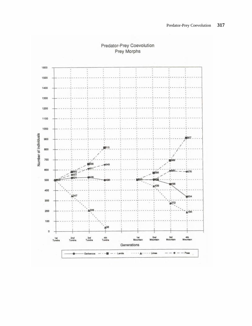
Tables 16.2 and 16.3 (pages 311 and 312) show the formulae associated with the worksheet calculations described in Appendix C and those associated with the new predator number conditionals described in Appendix D. APPENDIX F Sample Data Tables and Graphs The tables and graphs on pages 313–318 contain data derived at the morning session of my Predator-Prey Coevolution Workshop at the 1993 ABLE Conference in Toronto, Canada. The computer system was used a Macintosh IIsi with a Personal Laserwriter printer. The software used was Microsoft Excel 4.0.








Chapter 16 Predator-Prey Coevolution

Documents