Chapter 15: Time of Concentration - Irrigation ToolBoxirrigationtoolbox.com/NEH/Part630_Hydrology/NEH630-ch15draft.pdf · Chapter 15 Time of Concentration. ... its programs and activities

(210–VI–NEH, draft October 2008)

United StatesDepartment ofAgriculture

Natural ResourcesConservationService

Part 630 Hydrology National Engineering Handbook

Rain clouds

Cloud formation

Precipitation

Tran

spira

tion from

soi

l

f

rom

oce

an

Tran

spir

atio

n

OceanGround water

Rock

Deep percolation

SoilPercolation

Infiltration

Surface runoff

Evapora

tion fr

om ve

geta

tion

from

str

eam

s

Evaporation

Chapter 15 Time of Concentration

Part 630National Engineering Handbook

Time of ConcentrationChapter 15

(210–VI–NEH, draft October 2008)

Issued draft October 2008

The U.S. Department of Agriculture (USDA) prohibits discrimination in all its programs and activities on the basis of race, color, national origin, age, disability, and where applicable, sex, marital status, familial status, parental status, religion, sexual orientation, genetic information, political beliefs, re-prisal, or because all or a part of an individual’s income is derived from any public assistance program. (Not all prohibited bases apply to all programs.) Persons with disabilities who require alternative means for communication of program information (Braille, large print, audiotape, etc.) should con-tact USDA’s TARGET Center at (202) 720–2600 (voice and TDD). To file a complaint of discrimination, write to USDA, Director, Office of Civil Rights, 1400 Independence Avenue, SW., Washington, DC 20250–9410, or call (800) 795–3272 (voice) or (202) 720–6382 (TDD). USDA is an equal opportunity provider and employer.

(210–VI–NEH, draft October 2008) 15–i

Chapter 15 was originally prepared in 1971 by Kenneth M. Kent (retired). This version was prepared by Donald E. Woodward (retired), under the guidance of Claudia C. Hoeft, national hydraulic engineer, Washington, D.C. Annette Humpal, hydraulic engineer, Wisconsin, and Geoffrey Cer-relli, hydraulic engineer, Pennsylvania, provided the information in appen-dix 15B.

Acknowledgments



(210–VI–NEH, draft October 2008)15–ii

(210–VI–NEH, draft October 2008) 15–iii

Contents


630.1500 Introduction 15–1

630.1501 Definitions and basic relations 15–1

(a) Lag ..................................................................................................................15–1

(b) Time of concentration .................................................................................15–2

(c) Relation between lag and time of concentration .....................................15–2

630.1502 Methods for estimating time of concentration 15–3

(a) Watershed lag method .................................................................................15–3

(b) Velocity method ............................................................................................15–4

630.1503 Other considerations 15–7

(a) Field observations ........................................................................................15–7

(b) Surface flow ..................................................................................................15–7

(c) Travel time through bodies of water ..........................................................15–8

(d) Variation in lag and time of concentration ...............................................15–8

(e) Effects of urbanization ................................................................................15–8

(f) Geographic information systems ..............................................................15–9

630.1504 Examples 15–10

(a) Example of watershed lag method ..........................................................15–10

(b) Example of velocity method .....................................................................15–10

630.1505 References 15–14

Appendix 15A Other Methods for Computing Time of Concentration 15A–1

Appendix 15B Shallow Concentrated Flow Alternatives 15B–1

Appendix 15C Types of Flow 15C–1



(210–VI–NEH, draft October 2008)15–iv

Figures Figure 15–1 The relation of time of concentration (Tc) and 15–2lag (L) to the hydrograph

Figure 15–2 Velocity versus slope for shallow concentrated flow 15–6

Figure 15–3 Watershed map Falls Creek, Kent County, RI 15–10

Figure 15–4 Sample watershed 15–12

Figure 15B–1 Cerelli's shallow concentrated flow curves 15B–2

Figure 15B–2 TR–55 shallow concentrated flow curves 15B–3

Figure 15C–1 Types of flow 15C–1

Tables Table 15–1 Roughness coefficients for sheet flow 15–4

Table 15–2 Equations and assumptions developed from figure 15–2 15–5

Table 15–3 Maximum sheet flow lengths using the McCuen-Spiess 15–8Limitation Criteria

Table 15–4 Variation in lag time for selected events for selected 15–9streams in Maryland

Table 15–5 Field data and computed velocities at each cross 15–11section in reach R–2

Table 15–6 Field data and computed velocities and travel times 15–13for segments along reach R–4

Table 15B–1 Assumption used by Cerelli to develop shallow 15B–1concentrated flow curve

(210–VI–NEH, draft, October 2008)


630.1500 Introduction

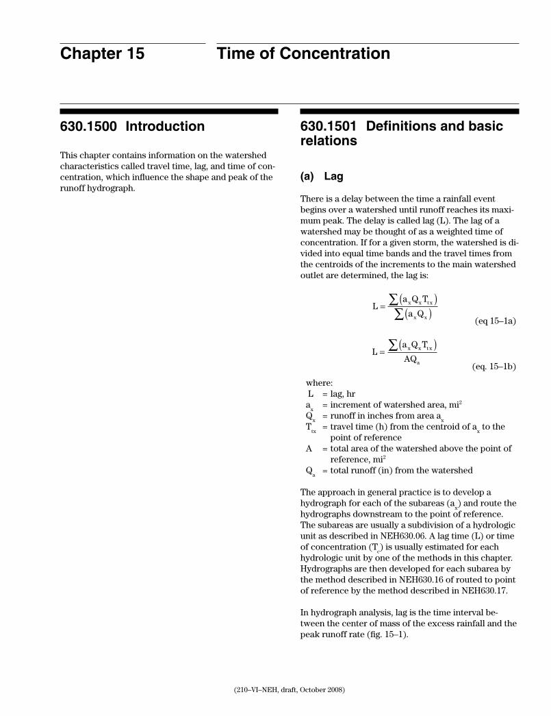
This chapter contains information on the watershed characteristics called travel time, lag, and time of con-centration, which influence the shape and peak of the runoff hydrograph.

630.1501 Definitions and basic relations

(a) Lag

There is a delay between the time a rainfall event begins over a watershed until runoff reaches its maxi-mum peak. The delay is called lag (L). The lag of a watershed may be thought of as a weighted time of concentration. If for a given storm, the watershed is di-vided into equal time bands and the travel times from the centroids of the increments to the main watershed outlet are determined, the lag is:

La Q T

a Qx x t x

x x

=( )

( )∑∑

(eq 15–1a)

La Q T

AQx x t x

a

=( )∑

(eq. 15–1b)

where: L = lag, hra

x = increment of watershed area, mi2

Qx

= runoff in inches from area ax

Ttx

= travel time (h) from the centroid of ax to the

point of referenceA = total area of the watershed above the point of

reference, mi2

Qa

= total runoff (in) from the watershed

The approach in general practice is to develop a hydrograph for each of the subareas (a

x) and route the

hydrographs downstream to the point of reference. The subareas are usually a subdivision of a hydrologic unit as described in NEH630.06. A lag time (L) or time of concentration (T

c) is usually estimated for each

hydrologic unit by one of the methods in this chapter. Hydrographs are then developed for each subarea by the method described in NEH630.16 of routed to point of reference by the method described in NEH630.17.

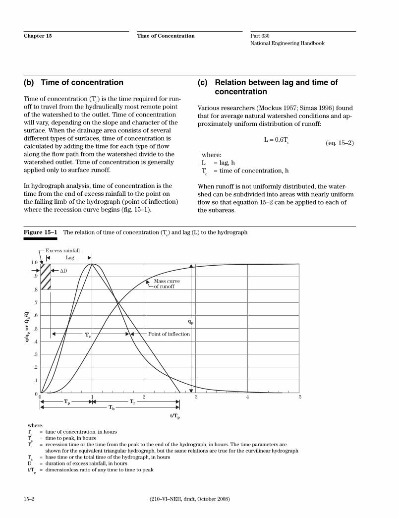
In hydrograph analysis, lag is the time interval be-tween the center of mass of the excess rainfall and the peak runoff rate (fig. 15–1).

Part 630 National Engineering Handbook


15–2 (210–VI–NEH, draft, October 2008)

(b) Time of concentration

Time of concentration (Tc) is the time required for run-

off to travel from the hydraulically most remote point of the watershed to the outlet. Time of concentration will vary, depending on the slope and character of the surface. When the drainage area consists of several different types of surfaces, time of concentration is calculated by adding the time for each type of flow along the flow path from the watershed divide to the watershed outlet. Time of concentration is generally applied only to surface runoff.

In hydrograph analysis, time of concentration is the time from the end of excess rainfall to the point on the falling limb of the hydrograph (point of inflection) where the recession curve begins (fig. 15–1).

(c) Relation between lag and time of concentration

Various researchers (Mockus 1957; Simas 1996) found that for average natural watershed conditions and ap-proximately uniform distribution of runoff:

L Tc= 0 6. (eq. 15–2)

where:L = lag, hT

c = time of concentration, h

When runoff is not uniformly distributed, the water-shed can be subdivided into areas with nearly uniform flow so that equation 15–2 can be applied to each of the subareas.

Figure 15–1 The relation of time of concentration (Tc) and lag (L) to the hydrograph

1.0

.9

.8

.7

.6

.5

.4

.3

.2

.1

0 0 1 2 3 4 5

q/q

p o

r Q

a/Q

t/Tp

Tp

Tc

qp

TrTb

Excess rainfall

∆D

Mass curveof runoff

Lag

Point of inflection

where: T

c = time of concentration, in hours

Tp

= time to peak, in hoursT

r = recession time or the time from the peak to the end of the hydrograph, in hours. The time parameters are

shown for the equivalent triangular hydrograph, but the same relations are true for the curvilinear hydrographT

b = base time or the total time of the hydrograph, in hours

D = duration of excess rainfall, in hourst/T

p = dimensionless ratio of any time to time to peak

Chapter 15

15–3(210–VI–NEH, draft, October 2008)

Time of Concentration Part 630 National Engineering Handbook

630.1502 Methods for estimating time of concentration

Two primary methods of computing time of concentra-tion were developed by the Soil Conservation Service (SCS), now the Natural Resources Conservation Service (NRCS).

(a) Watershed lag method

The SCS method for watershed lag was developed by Mockus in 1961. It spans a broad set of conditions ranging from heavily forested watersheds with steep channels and a high percent of the runoff resulting from subsurface flow, to meadows providing a high retardance to surface runoff, to smooth land surfaces and large paved areas.

L

S

Y=

+( )

0 8 0 7

0 51900

. .

. (eq. 15–3a)

Applying equation 15–2 yields:

T

S

Yc =+( )

0 8

0 7

0 5

1

1140.

.

.

(eq. 15–3b)

where:L = lag, hT

c = time of concentration, h = flow length, ftY = average watershed land slope, percentS = maximum potential retention, in

=′

−1 000

10,

cn

where: cn′ = the retardance factor

Flow length ( )—Flow length is defined as the path along which water flows from the watershed divide to the outlet. Flow length can be measured using aerial photographs, quadrangle sheets, or GIS techniques. Mockus (1973) developed a relationship between flow length and drainage area characteristics using data from Agricultural Research Service (ARS) watersheds. This relationship is:

= 209 0 6A . (eq. 15–4)

where: = flow length, ftA = drainage area, acres

Land slope (Y), in percent—The average land slope of the watershed, not to be confused with the slope of the flow path. The average land slope for small water-sheds can be determined several different ways:

• byassuminglandslopeisequaltothesoilmapunit slope, from the soil survey

• byusingaclinometer,asmeasuredinthefield

• bydrawingthreetofourlinesonatopographicmap perpendicular to the contour lines and determining the average slope of these lines

• bydeterminingtheaverageofthelandslopefrom grid points using a dot counter

• byusingthefollowingequation(Chow1964):

Y

MN

A=

( )100

(eq. 15–5)

where:Y = average land slope, in percent

M = summation of the length of the contour lines that pass through the watershed drainage area on the quad sheet, ft

N = contour interval used, ftA = drainage area, ft2

(1 acre = 43,560 ft2)

Retardance factor—The retardance factor, cn′, is a measure of surface conditions relating to the rate at which runoff concentrates at some point of interest. The retardance factor is approximately the same as the curve number (CN) as defined in NEH630.09.

Thick mulches in forests are associated with low retardance factors and reflect high degrees of retar-dance, as well as high infiltration rates. Hay meadows have relatively low retardance factors. Like thick mulches in forests, stem densities in meadows provide a high degree of retardance to overland flow in small watersheds. Conversely, bare surfaces with very little retardance to overland flows are represented by high retardance factors.




In practical usage, the runoff curve number (CN) is used as a surrogate for cn′, and the CN tables in NEH630.09 can be used to approximate the retardance factor, S, in equations 15–3a and 15–3b. A CN of less than 50 or greater than 95 should not be used in the solution of equation 15–3a and 15–3b.

Applications and limitations—The watershed lag equation was developed from data from 24 watersheds ranging in size from 1.3 acres to 9.2 square miles, with the majority less than 2,000 acres in size (Mockus 1961). Folmar and Miller (2000) revisited the develop-ment of this equation using additional watershed data and found that 5 to 19 square miles may be a more realistic upper limit.

(b) Velocity method

Another method for determining time of concentra-tion normally used within NRCS is called the velocity method. The velocity method assumes that time of concentration is the sum of travel times for segments along the hydraulically most remote flow path.

T T T T Tc t t t tn= + + +1 2 3 (eq. 15–6)

where:T


Tt = travel time of a segment, h

n = number of segments comprising the total hy-draulic length

The segments used in the velocity method may be of three types: sheet flow, shallow concentrated flow, and open channel flow.

The travel time for any given segment is equal to:

T

Vt =

3600 (eq. 15–7)

where:T

t = travel time, h = flow length, ftV = average velocity, ft/s3600 = a conversion factor (seconds to hours)

Sheet flow—Sheet flow is flow over plane surfaces. It usually occurs in the headwaters of a stream.

A simplified version of the Manning’s kinematic solu-tion may be used to compute travel time for sheet flow. This simplification of the kinematic equation was developed by Welle and Woodward (1986) after study-ing the impact of various parameters on the estimates.

TP S

t =( )

( )

0 0070 8

2

0 5 0 4

..

. .

n

(eq. 15–8)

where:T

t = travel time, h

n = roughness coefficient (table 15–1) = flow length, ftP

2 = 2-year, 24-hour rainfall, in

S = slope of hydraulic grade line, ft/ft

Table 15–1 Roughness coefficients for sheet flow (flow depth generally ≤ 0.1 feet)

Surface description n1

Smooth surface (concrete, asphalt, gravel, or bare soil) ..........................................................................0.011

Fallow (no residue) ............................................................0.05

Cultivated soils:

Residue cover ≤ 20% .......................................................0.06 Residue cover > 20% .......................................................0.17

Grass:

Short grass priarie ..........................................................0.15 Dense grasses2 .................................................................0.24 Bermudagrass .................................................................0.41

Range (natural) ...................................................................0.13

Woods:3

Light underbrush ..........................................................0.40 Dense underbrush 0.80

1 The n values are a composite of information compiled by Eng-man (1986)

2 Includes species such as weeping lovegrass, bluegrass, buffa-lograss, blue gramma grass, and native grass mixtures

3 When selecting n, consider cover to a height of about 0.1 ft. This is the only part of the plant cover that will obstruct sheet flow.

Chapter 15



This simplified form of Manning’s kinematic solution is based on the following assumptions:

• shallowsteadyuniformflow

• constantrainfallexcessintensity(thatpartofa rain available for runoff) both temporal and spatial

• rainfalldurationof24hours

• minoreffectofinfiltrationontraveltime

For sheet flow, the roughness coefficient is an effective roughness coefficient that includes the effects of rough-ness and the effects of raindrop impact including drag over the surface; obstacles such as litter, crop ridges, and rocks; and erosion and transport of sediment. These n values are only applicable for flow depths of approximately 0.1 foot or less, where sheet flow is said to occur. Table 15–1 gives roughness coefficient values for sheet flow for various surface conditions.

Shallow concentrated flow—After approximately 100 feet, sheet flow usually becomes shallow concen-trated flow collecting in swales, small rills, and gullies. Shallow concentrated flow is not assumed to have a well-defined channel. Velocities are developed using wide, rectangular channel flow concepts. Average velocity for shallow concentrated flow can be deter-mined using figure 15–2, in which average velocity is a function of watercourse slope and type of channel (Kent 1964). For slopes less than 0.005 foot per foot, the equations in table 15–2 may be used.

After estimating average velocity using figure 15–2, use equation 15–7 or the equations in table 15–2 to estimate travel time for the shallow concentrated flow segment.

It is assumed that shallow concentrated flow can be represented by one of seven flow types. The curves in figure 15–2 were used to develop the information in table 15–2.

Open channel flow—Open channels are assumed to begin where surveyed cross-sectional information has been obtained, where channels are visible on aerial photographs, or where blue lines (indicating streams) appear on U.S. Geological Survey (USGS) quadrangle sheets. Manning’s equation or water surface profile in-formation can be used to estimate average flow veloc-ity. Average flow velocity is usually determined for the bankfull elevation.

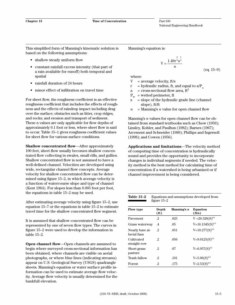
Manning’s equation is:

Vr s

=1 49

23

12.

n (eq. 15–9)

where:V = average velocity, ft/sr = hydraulic radius, ft, and equal to a/P

wa = cross-sectional flow area, ft2

Pw = wetted perimeter, ft

s = slope of the hydraulic grade line (channel slope), ft/ft

n = Manning’s n value for open channel flow

Manning’s n values for open channel flow can be ob-tained from standard textbooks such as Chow (1959); Linsley, Kohler, and Paulhus (1982); Barnes (1967); Arcement and Schneider (1989); Phillips and Ingersoll (1998); and Cowen (1956).

Applications and limitations—The velocity method of computing time of concentration is hydraulically sound and provides the opportunity to incorporate changes in individual segments if needed. The veloc-ity method is the best method for calculating time of concentration if a watershed is being urbanized or if channel improvement is being considered.

Flow type Depth (ft)

Manning’s n Equation (ft/s)

Pavement .2 .025 V =20.328(S)0.5

Grass waterway .4 .05 V=16.1345(S)0.5

Nearly bare al-luvial fans

.2 .051 V=10.277(S)0.5

Cultivated straight row

.2 .056 V=9.0125(S)0.5

Short-grass pasture

.2 .07 V=6.957(S)0.5

Trash fallow .2 .101 V=5.06(S)0.5

Forest .2 .175 V=2.53(S)0.5

Table 15–2 Equations and assumptions developed from figure 15–2




Figure 15–2 Velocity versus slope for shallow concentrated flow

Cul

tivat

ed, s

trai

ght r

ow

Min

imum

tilla

ge c

ultiv

atio

n; c

onto

ur o

r st

rip

crop

ped

and

woo

dlan

d

90807060

50

40

30

20

109876

5

4

3

Fore

st w

ith h

eavy

gro

und

litte

r an

d ha

y m

eado

w

Shor

t gra

ss p

astu

re

Nea

rly

bare

and

unt

illed

and

allu

vial

fans

wes

tern

mou

ntai

n re

gion

s

Gra

ssed

wat

erw

ay

Pave

d ar

ea s

tree

t flo

w a

nd s

mal

l upl

and

gulli

es

2

1.0

0.5

Velocity (ft/s)

Slo

pe

(%)

0.1

0.2

0.3

0.4

0.5

0.6

0.7

0.8

0.9

1.0 2 3 4 5 6 7 8 9 10 15 20

100

Chapter 15



The channel length can be considered to represented by the blue line length on a 15- or 30-minute quad sheet. This length represents an average flow length for a wide range of storms.

Use the average velocity and the valley length of the reach to compute the travel time through the reach by equation 15–7. If the stream is quite sinuous, the chan-nel length and valley length may be significantly dif-ferent. Use whichever is more appropriate for the flow depth of the event being evaluated.

Manning’s kinematic solution should not be used for sheet flow lengths greater than 100 feet. Equation 15–8 was developed for use with the standard NRCS rainfall intensity-duration relationships and will work with the new NOAA atlases dated 2002 and forward. It was also developed assuming the 2-year, 24-hour precipitation value would be used.

Time of concentration calculations are based on the 2-year frequency discharge or bankfull discharge. Con-sidering the variation in all the variables that impact time of concentration in a watershed, it is normally assumed that the time of concentration computed us-ing 2-year characteristics is representative of the travel time conditions for a wide range of frequencies.

When combinations of flow occur together, a com-pound hydrograph with more than one peak and lag time may result. Ideally, the various types of flow should be separated for lag analysis and combined at the end of the study. In practice, lag is usually deter-mined only for the direct runoff portion of flow.

The role of channel and valley storage is inportant in the development and translation of a flow wave and the estimation of lag. Both the hydraulics and storage may change from storm to storm with velocity distri-bution varying greatly both horizontally and vertically. As a result, an average lag may have a large variation.

For multiple subarea watersheds, the time of concen-tration must be computed for each subarea individu-ally and consideration must be given to the travel time through downstream subareas from upstream subareas.

630.1503 Other considerations

(a) Field observations

For an accurate estimate of the time of concentra-tion, field observations of significant factors should be made. These include:

• thetypeofmaterialinthebanksandbottomofthe channel

• anestimateofManning’sn value

• conditionofvegetationinthechannelanditsflood plain

• slopeofthechannelbed

• presenceofanysignificantobstructions

When the time of concentration is needed as part of calculations for a specific design, sufficient surveys and observations should be made to ascertain that the values used for calculations are realistic. When the time of concentration is needed for preliminary con-clusions, the time of concentration may be estimated by taking travel distances from maps or aerial photo-graphs. This may involve velocity estimates based on general knowledge of approximate sizes and charac-teristics for channels in the geographic area.

(b) Surface flow

Both of the standard methods, as well as most other methods, assume that flow reaching the channel as surface flow or quick return flow adds directly to the peak of the subarea hydrograph. Locally derived pro-cedures might be developed from data where a major portion of the contributing flow is other than surface flow. This is normally determined by making a site visit to the watershed.

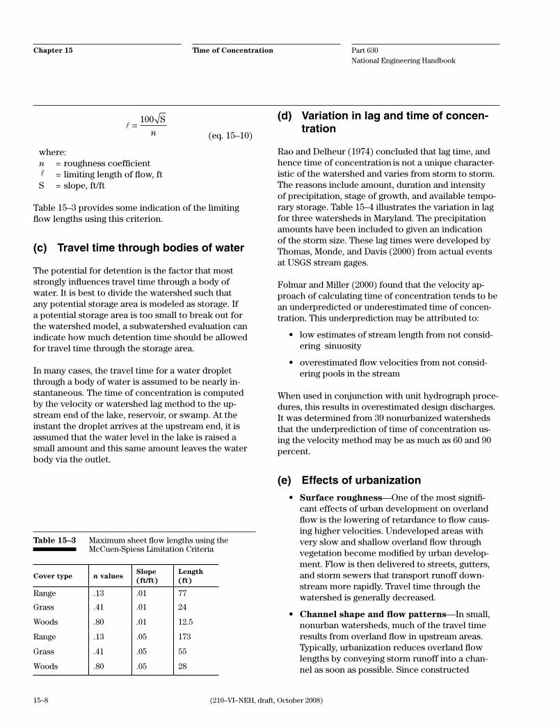
Kibler and Aron (1982) and others indicated the maxi-mum sheet flow length is less than 100 feet. McCuen and Spiess (1995) indicated that use of flow length as the limiting variable in the equation 15–8 could lead to less accurate designs. They indicated that the limita-tion should instead be based on:




=

100 S

n (eq. 15–10)

where:n = roughness coefficient = limiting length of flow, ftS = slope, ft/ft

Table 15–3 provides some indication of the limiting flow lengths using this criterion.

(c) Travel time through bodies of water

The potential for detention is the factor that most strongly influences travel time through a body of water. It is best to divide the watershed such that any potential storage area is modeled as storage. If a potential storage area is too small to break out for the watershed model, a subwatershed evaluation can indicate how much detention time should be allowed for travel time through the storage area.

In many cases, the travel time for a water droplet through a body of water is assumed to be nearly in-stantaneous. The time of concentration is computed by the velocity or watershed lag method to the up-stream end of the lake, reservoir, or swamp. At the instant the droplet arrives at the upstream end, it is assumed that the water level in the lake is raised a small amount and this same amount leaves the water body via the outlet.

(d) Variation in lag and time of concen-tration

Rao and Delheur (1974) concluded that lag time, and hence time of concentration

is not a unique character-

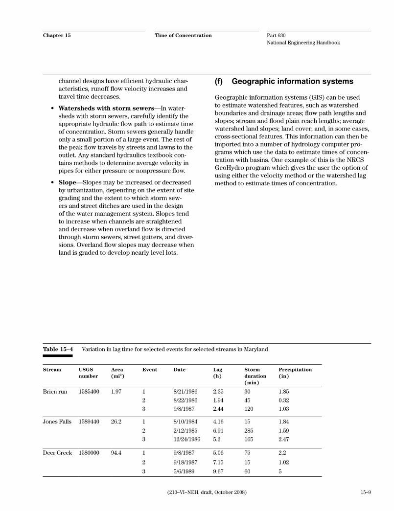
istic of the watershed and varies from storm to storm. The reasons include amount, duration and intensity of precipitation, stage of growth, and available tempo-rary storage. Table 15–4 illustrates the variation in lag for three watersheds in Maryland. The precipitation amounts have been included to given an indication of the storm size. These lag times were developed by Thomas, Monde, and Davis (2000) from actual events at USGS stream gages.

Folmar and Miller (2000) found that the velocity ap-proach of calculating time of concentration tends to be an underpredicted or underestimated time of concen-tration. This underprediction may be attributed to:

• lowestimatesofstreamlengthfromnotconsid-ering sinuosity

• overestimatedflowvelocitiesfromnotconsid-ering pools in the stream

When used in conjunction with unit hydrograph proce-dures, this results in overestimated design discharges. It was determined from 39 nonurbanized watersheds that the underprediction of time of concentration us-ing the velocity method may be as much as 60 and 90 percent.

(e) Effects of urbanization

• Surface roughness—One of the most signifi-cant effects of urban development on overland flow is the lowering of retardance to flow caus-ing higher velocities. Undeveloped areas with very slow and shallow overland flow through vegetation become modified by urban develop-ment. Flow is then delivered to streets, gutters, and storm sewers that transport runoff down-stream more rapidly. Travel time through the watershed is generally decreased.

• Channel shape and flow patterns—In small, nonurban watersheds, much of the travel time results from overland flow in upstream areas. Typically, urbanization reduces overland flow lengths by conveying storm runoff into a chan-nel as soon as possible. Since constructed

Cover type n valuesSlope (ft/ft)

Length (ft)

Range .13 .01 77

Grass .41 .01 24

Woods .80 .01 12.5

Range .13 .05 173

Grass .41 .05 55

Woods .80 .05 28

Table 15–3 Maximum sheet flow lengths using the McCuen-Spiess Limitation Criteria

Chapter 15



channel designs have efficient hydraulic char-acteristics, runoff flow velocity increases and travel time decreases.

• Watersheds with storm sewers—In water-sheds with storm sewers, carefully identify the appropriate hydraulic flow path to estimate time of concentration. Storm sewers generally handle only a small portion of a large event. The rest of the peak flow travels by streets and lawns to the outlet. Any standard hydraulics textbook con-tains methods to determine average velocity in pipes for either pressure or nonpressure flow.

• Slope—Slopes may be increased or decreased by urbanization, depending on the extent of site grading and the extent to which storm sew-ers and street ditches are used in the design of the water management system. Slopes tend to increase when channels are straightened and decrease when overland flow is directed through storm sewers, street gutters, and diver-sions. Overland flow slopes may decrease when land is graded to develop nearly level lots.

(f) Geographic information systems

Geographic information systems (GIS) can be used to estimate watershed features, such as watershed boundaries and drainage areas; flow path lengths and slopes; stream and flood plain reach lengths; average watershed land slopes; land cover; and, in some cases, cross-sectional features. This information can then be imported into a number of hydrology computer pro-grams which use the data to estimate times of concen-tration with basins. One example of this is the NRCS GeoHydro program which gives the user the option of using either the velocity method or the watershed lag method to estimate times of concentration.

Stream USGS number

Area (mi2)

Event Date Lag (h)

Storm duration (min)

Precipitation (in)

Brien run 1585400 1.97 1 8/21/1986 2.35 30 1.85

2 8/22/1986 1.94 45 0.32

3 9/8/1987 2.44 120 1.03

Jones Falls 1589440 26.2 1 8/10/1984 4.16 15 1.84

2 2/12/1985 6.91 285 1.59

3 12/24/1986 5.2 165 2.47

Deer Creek 1580000 94.4 1 9/8/1987 5.06 75 2.2

2 9/18/1987 7.15 15 1.02

3 5/6/1989 9.67 60 5

Table 15–4 Variation in lag time for selected events for selected streams in Maryland




630.1504 Examples

(a) Example of watershed lag method

Compute the time of concentration using the water-shed lag method for Falls Creek in Kent County, Rhode Island. The topographic map for the watershed is shown in figure 15–3. The watershed has the following attributes:

Drainage area, A = 0.42 mi2

Curve number, CN = 63–used as a surrogate for cn′

Longest flow path, = 1,100 ft

Watershed slope, Y = 4.81%

Time of concentration is computed using equation 15–3b:

T

S

Yc =+( )

0 8

0 7

0 5

1

1140.

.

.

Scn

S

S

=′

−

=

−

=

100010

1000

6310

5 87.

T

T

c

c

=( ) +( )

( )( )−

=

1100 5 87 1

1140 4 8110

0 42

0 8 0 7

0 5

. .

.

.

.

. h

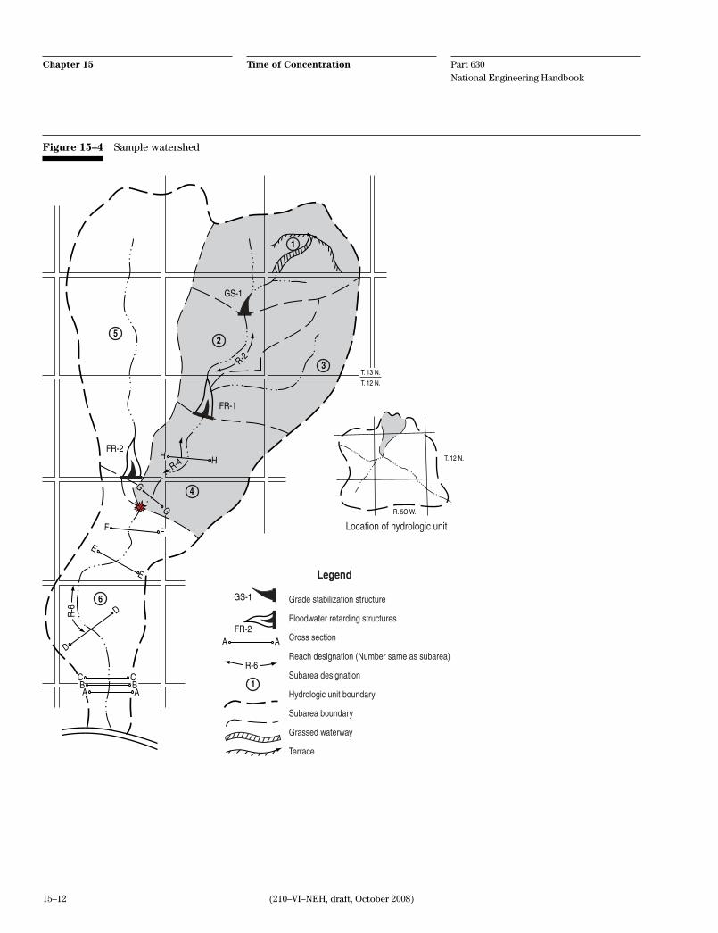
(b) Example of velocity method

For the watershed shown in figure 15–4, compute the time of concentration for that portion of the watershed above the junction of subareas 4 and 5 (red dot on fig-ure), consisting of subareas 1, 2, 3, and 4 (the shaded area on fig. 15–4). Assume that floodwater retarding structure, FR–1, has not been installed. The 2–year, 24-hour precipitation for watershed is 3.6 inches. Stream hydraulics have been computed using methods outlined in NEH630.14 for all the stream reaches. The flow lengths are:

GS–1 to confluence of subareas 2 and 3 6,000 feet

FR–1 to HH 2,400 feet

HH to GG 2,800 feet

GG to confluence of subareas 4 and 5 900 feet

Total 12,100 feetFigure 15–3 Watershed map Falls Creek, Kent County, RI

Chapter 15



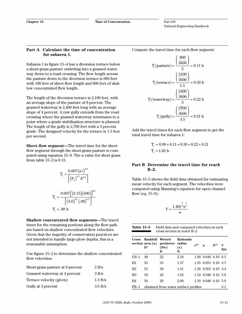
Part A Calculate the time of concentration for subarea 1.

Subarea 1 in figure 15–4 has a diversion terrace below a short-grass pasture outletting into a grassed water-way down to a road crossing. The flow length across the pasture down to the diversion terrace is 900 feet with 100 feet of sheet flow length and 800 feet of shal-low concentrated flow length.

The length of the diversion terrace is 2,100 feet, with an average slope of the pasture of 8 percent. The grassed waterway is 2,400 feet long with an average slope of 4 percent. A raw gully extends from the road crossing where the grassed waterway terminates to a point where a grade stabilization structure is planned. The length of the gully is 2,700 feet with a 3 percent grade. The designed velocity for the terrace is 1.5 feet per second.

Sheet flow segment—The travel time for the sheet flow segment through the short-grass pasture is com-puted using equation 15–8. The n value for short grass from table 15–2 is 0.15.

Tn

P St =

( )( )

0 0070 8

2

0 5 0 4

..

. .

T

T

t

t

=( )( )

( ) ( )

=

0 007 0 15 100

3 6 08

09

0 8

0 5 0 4

. .

. .

.

.

. .

h

Shallow concentrated flow segments—The travel times for the remaining portions along the flow path are based on shallow concentrated flow velocities. Given that the majority of conservation practices are not intended to handle large plow depths, this is a reasonable assumption.

Use figure 15–2 to determine the shallow concentrated flow velocities.

Short-grass pasture at 8 percent 2 ft/s

Grassed waterway at 4 percent 3 ft/s

Terrace velocity (given) 1.5 ft/s

Gully at 3 percent 3.5 ft/s

Compute the travel time for each flow segment:

T

T

t

t

(pasture) h

(terrace)

=

=

=

8003600

20 11

21003600

.

=

=

=

=

1 50 39

24003600

30 22

2

..

.

h

(waterway) h

(gully)

T

T

t

t

77003600

3 50 21

=.

. h

Add the travel times for each flow segment to get the total travel time for subarea 1:

T

Tt

t

= + + + +=

0 09 0 11 0 39 0 22 0 21

1 02

. . . . .

. h

Part B Determine the travel time for reach R–2.

Table 15–5 shows the field data obtained for estimating mean velocity for each segment. The velocities were computed using Manning's equation for open channel flow (eq. 15–9):

Vr s

=1 49

23

12.

n

Cross section

Bankfull area (a) ft2

Wetted perimeter (Pw) ft

Hydraulic radius (r) ft

r2/3 n S1/2 V ft/s

GS–1 48 22 2.18 1.68 0.040 0.10 6.3

H1 55 35 1.57 1.35 0.055 0.10 3.7

H2 55 39 1.41 1.26 0.055 0.10 3.4

H3 50 26 1.92 1.54 0.040 0.10 5.8

H4 56 28 2.00 1.59 0.040 0.10 5.9

FR–1 obtained from water surface profiles 6.1

Table 15–5 Field data and computed velocities at each cross section in reach R–2




Legend

Location of hydrologic unit

Grade stabilization structure

Floodwater retarding structures

Cross section

Reach designation (Number same as subarea)

Subarea designation

Hydrologic unit boundary

Subarea boundary

Grassed waterway

Terrace

CBA

C

D

D

E

E

G

G

FF

HH

BA

AA

2

FR-2

R-6

FR-2

GS-1

R-6

R-4

R-2

FR-1

T. 13 N.

T. 12 N.

T. 12 N.

R. 5O W.

GS-1

3

1

5

4

6

1

Figure 15–4 Sample watershed

Chapter 15



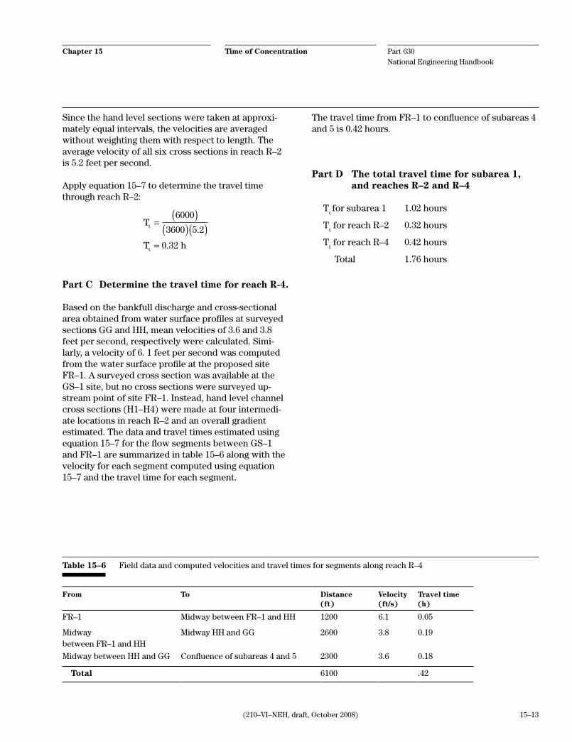
Since the hand level sections were taken at approxi-mately equal intervals, the velocities are averaged without weighting them with respect to length. The average velocity of all six cross sections in reach R–2 is 5.2 feet per second.

Apply equation 15–7 to determine the travel time through reach R–2:

T

T

t

t

=( )

( )( )=

6000

3600 5 2

0 32

.

. h

Part C Determine the travel time for reach R-4.

Based on the bankfull discharge and cross-sectional area obtained from water surface profiles at surveyed sections GG and HH, mean velocities of 3.6 and 3.8 feet per second, respectively were calculated. Simi-larly, a velocity of 6. 1 feet per second was computed from the water surface profile at the proposed site FR–1. A surveyed cross section was available at the GS–1 site, but no cross sections were surveyed up-stream point of site FR–1. Instead, hand level channel cross sections (H1–H4) were made at four intermedi-ate locations in reach R–2 and an overall gradient estimated. The data and travel times estimated using equation 15–7 for the flow segments between GS–1 and FR–1 are summarized in table 15–6 along with the velocity for each segment computed using equation 15–7 and the travel time for each segment.

The travel time from FR–1 to confluence of subareas 4 and 5 is 0.42 hours.

Part D The total travel time for subarea 1, and reaches R–2 and R–4

Tt for subarea 1 1.02 hours

Tt for reach R–2 0.32 hours

Tt for reach R–4 0.42 hours

Total 1.76 hours

From To Distance (ft)

Velocity (ft/s)

Travel time (h)

FR–1 Midway between FR–1 and HH 1200 6.1 0.05

Midway between FR–1 and HH

Midway HH and GG 2600 3.8 0.19

Midway between HH and GG Confluence of subareas 4 and 5 2300 3.6 0.18

Total 6100 .42

Table 15–6 Field data and computed velocities and travel times for segments along reach R–4




630.1505 References

Arcement, G.J., and V.R. Schneider. 1989. Guide for selecting Manning’s roughness coefficient for natural channel and flood plains. U.S. Geological Survey Water Supply Paper 2339.

Barnes Jr., H H. 1967. Roughness characteristics of natural channels. U.S. Geological Survey Water Supply Paper 1849.

Cerrelli, G.A. 1990. Professional notes. Unpublished data. U.S. Department of Agriculture, Natural Resources Conservation Service. Annapolis, MD.

Cerrelli, G.A. 1992. Professional notes. Unpublished data. U.S. Department of Agriculture, Natural Resources Conservation Service. Annapolis, MD.

Chow, V.T. 1959. Open-channel hydraulics. McGraw-Hill Book. Inc. Company. New York, NY.

Chow, V.T. 1964. Handbook of applied hydrology. McGraw Hill Book, Inc. Company New York, NY.

Cowen, W.L. 1956. Estimating hydraulic roughness coefficients. Agricultural Engineering. Vol. 378, No. 7. pp. 473–475.

Engman, E.T. 1986. Roughness coefficients for routing surface runoff. J. of Irrigation and Drainage Engi-neering 112 (1). ASCE. New York, NY. pp. 39–53.

Folmar, N.D., and A.C. Miller. 2000. Historical perspective of the NRCS lag time equation, Transportation Research Board. Seventieth an-nual meeting. Washington, DC.

Kent, K.M. 1964. Chapter 15 documentation. U.S. Dept. of Agriculture, Soil Conservation Service. Wash-ington, DC.

Kerby, W.S. 1959. Time of concentration for overland flow. J. of Civil Engineering 26(3). ASCE. Reston, VA. pp. 60.

Kirpich, Z.P. 1940. Time of concentration of small watersheds. J. of Civil Engineering 10(6). ASCE. New York, NY. pp. 362.

Kibler, D.F. 1980. Personnel communication

Kibler, D.F., and G. Aron. 1982. Estimating basin lag and T

c in small urban watershed. Paper presented

at the spring meeting American Geophysical Union. Philadelphia, PA.

Linsley, R.K., M.A. Kohler, and J.L. Paulhus. 1982. Hy-drology for engineers. Third edition McGraw-Hill Book Company, Inc. New York, NY.

McCuen, R.H., and J.M. Spiess. 1995. Assessment of kinematic wave time of concentration. J. of Hy-draulic Engineering. ASCE. Reston, VA.

Mockus, V. 1961. Watershed lag. ES–1015. U.S. Dept. of Agriculture, Soil Conservation Service. Washing-ton, DC.

Mockus, V. 1957. Use of storm and watershed char-acteristics in synthetic hydrograph analysis and application. Paper presented at the annual meet-ing of AGU Pacific Southwest Region.

Mockus, V. 1973. A method for estimating volume and rate of runoff in small watersheds. U.S. Dept. of Agriculture, Soil Conservation Service. Washing-ton, DC.

Papadakis, C., and N. Kazan. 1986. Time of concentra-tion in small rural watersheds. Technical report 101/08/86/CEE. College of Engineering, Univer-sity of Cincinnati. Cincinnati, OH.

Phillips, J.V., and T.L. Ingersoll. 1998. Verification of roughness coefficients for selected natural and constructed stream channels in Arizona. U.S. Geological Survey paper 1584.

Rao A.R., and J.W. Delheur. 1974. Instantaneous unit hydrographs, peak discharges, and time lags in urban areas. Hydrologic Sciences Bulletin, Vol. 19, No. 2. pp. 185–198.

Sheridan, J.M. 1994. Hydrograph time parameters for flatland watershed. Trans. of ASAE. St. Joseph, MI.

Chapter 15



Simas, M. 1996. Lag time characteristics in small watershed in the United States. A dissertation submitted to School of Renewable Natural Re-sources, University of Arizona. Tucson, AZ.

Thomas, W.O. Jr., M.C. Monde, and S.R. Davis. 2000. Estimation of time of concentration for Mary-land streams. Transportation Research No. 1720, Transportation Research Board, National Research Council, National Academy Press, Washington, DC, pp 95–99.

U.S. Department of Agriculture, Natural Resources Conservation Service. 2007. National Engineering Handbook, Part 630, Chapter 16, Hydrographs. Washington, D.C.

U.S. Department of Agriculture, Natural Resources Conservation Service. 2004. National Engineering Handbook, Part 630, Chapter 9, Hydrologic soil-cover complexes. Washington, D.C.

U.S. Department of Agriculture, Natural Resources Conservation Service. 2001. National Engineering Handbook, Part 630, Chapter 17, Flood routing. Washington, D.C.

U.S. Department of Agriculture, Natural Resources Conservation Service. 1999. National Engineering Handbook, Part 630, Chapter 6, Stream reaches and hydrologic units. Washington, D.C.

U.S. Department of Agriculture, Natural Resources Conservation Service. 1986. Technical release number 55, urban Hydrology for small water-sheds. Washington, D.C.

Welle, P.J., and D.E. Woodward. 1986. Time of concen-tration. Hydrology, Technical Note No. N4. U.S. Dept. of Agriculture, Soil Conservation Service, NENTC. Chester, PA.




(210–VI–NEH, draft, October 2008)

This appendix includes procedures developed by users that may have application for NRCS in limited areas or special studies.

Various regression equations have been developed by various agencies that work well to estimate travel times or times of concentration for the regions used in their development. In general, these equations are for existing conditions and cannot be adapted to future condition or urbanization. These equations are includ-ed for information.

Please note that whenever possible an effort was made to maintain the form of equations as published by the author. Therefore, the various methods illustrated here may use different units.

Kirpich equation—The Kirpich (1940) equation was developed using data from seven rural watersheds in Tennessee with well-defined channels and steep slopes.

T Sc = −0 0078 0 77 0 385. . . (eq. 15A–1)

For small watersheds in Pennsylvania, the Kirpich equation is similar, but not identical.

T Sc = −0 0013 0 77 0 385. . . (eq. 15A–2)

where:T

c = time of concentration, min

= length of channel from headwater to outlet, ftS = slope of the longest hydraulic length, ft/ft

Drainage area equations—These equations taken from a 1957 version of NEH–4, were developed using small watershed data.

The following equation was developed from small watershed data in Texas:

T Ac = 2 4 0 6. .

(eq. 15A–3)

The following equation was developed from small watershed data in Ohio.

T Ac = 0 9 0 6. .

(eq. 15A–4)

The following equation was developed from Coshoc-ton, Ohio, small watershed data.

T Ac = 0 5 0 6. .

(eq. 15A–5)

where: T


A = drainage area, mi2

Simas equations—Simas (1996), in an analysis of 116 small agricultural watersheds, developed several re-gression equations for watershed lag. Lag was defined by Simas as the time between the centroid of effective rainfall and the centroid of direct runoff. Equations were modified to time of concentration using the re-lationship of lag = 0.6Tc or Tc = 1.67 Lag. It was found that this relationship was reasonable and consistent with information in NEH630.15.

The simplest form of the equation Simas developed is:

T Ac = 0 0418 0 324. .

(eq. 15A–6)

where:T


A = the drainage area, acre

The statistically most significant equation Simas devel-oped is:

T W S Sc nat= −0 0085 0 594 0 1505 0 3131. . . .

(eq. 15A–7)

where:T


W = watershed width, ft (area ft2/length ft)S = average watershed slope, ft/ft

Snat

= watershed storage and is a function of curve number

where: S

nat = (1000/CN)–10

Sheridan equation—Sheridan (1994) performed a study on nine flatland watersheds located in Georgia and Florida. A regression analysis was performed us-ing many basin characteristics to determine a timing equation. However, it was found that the main chan-nel length was the overwhelming characteristic that

Appendix 15A Other Methods for Computing Time of Concentration



15A–2 (210–VI–NEH, draft, October 2008)

correlated with the timing parameter. Therefore, an equation was developed based solely on main channel length to estimate the time of concentration. The equa-tion had a correlation coefficient (R2) of 96 percent.

Tc = 2 20 92. . (eq. 15A–8)

where:T


= main channel length, km

Folmar and Miller equation—Folmar and Miller (2000) developed an equation for lag time from 54 watersheds throughout the country. Lag was measured from the centroid of excess precipitation to the peak of the hydrograph. Watersheds ranged in size from approximately 3 acres to 20 square miles. Similar to what was determined by Sheridan (1994), it was found that only the longest hydraulic length as determined by comparing travel time was needed to determine an estimate of lag time, and that the watershed slope and curve number were not needed to estimate lag time. The developed equation had an R2 value of 85 percent.

Tl =

0 63

141

.

(eq. 15A–9)

where:T

l = lag time, h

= longest hydraulic length, ft

Papadakis and Kazan—Papadakis and Kazan (1986), from the University of Cincinnati, developed regres-sion equations using data from 84 small ARS water-sheds across the United States.

T L S ic = − −0 66 0 5 0 52 0 31 38. . . . .n (eq. 15A–10)

where:T

c = time of concentration, min

L = length of the longest waterway, ftS = slope of the flow path, %i = intensity of the rainfall excess, in/hn = roughness coefficient (Manning’s n value for

channel)

(210–VI–NEH, draft, July 2008)

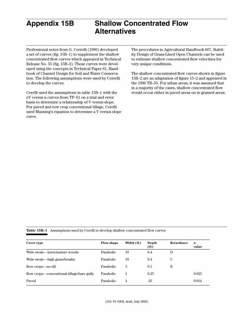
Professional notes from G. Cerrelli (1990) developed a set of curves (fig. 15B–1) to supplement the shallow concentrated flow curves which appeared in Technical Release No. 55 (fig. 15B–2). These curves were devel-oped using the concepts in Technical Paper 61, Hand-book of Channel Design for Soil and Water Conserva-tion. The following assumptions were used by Cerrelli to develop the curves.

Cerelli used the assumptions in table 15B–1 with the nV versus n curves from TP–61 on a trial and error basis to determine a relationship of V versus slope. For paved and row crop conventional tillage, Cerelli used Manning's equation to determine a V versus slope curve.

Appendix 15B Shallow Concentrated Flow Alternatives

The procedures in Agricultural Handbook 667, Stabil-ity Design of Grass-Lined Open Channels can be used to estimate shallow concentrated flow velocities for very unique conditions.

The shallow concentrated flow curves shown in figure 15B–2 are an adaptation of figure 15–2 and appeared in the 1986 TR–55. For urban areas, it was assumed that in a majority of the cases, shallow concentrated flow would occur either in paved areas on in grassed areas.

Cover type Flow shape Width (ft) Depth (ft)

Retardance n value

Wide swale—lawn/mature woods Parabolic 10 0.4 D

Wide swale—high grass/brushy Parabolic 10 0.4 C

Row crops—no till Parabolic 3 0.1 E

Row crops—conventional tillage/bare gully Parabolic 1 0.25 0.025

Paved Parabolic 4 .35 0.014

Table 15B–1 Assumptions used by Cerelli to develop shallow concentrated flow curves



15B–2 (210–VI–NEH, draft, July 2008)

6 7 8 9

.05.001

.005

.01

.05

Row

cro

ps–n

o til

l

Wid

e br

ushy

sw

ale

Wid

e sw

ale

low

veg

etat

ion

Row

cro

ps–c

onv.

till

Slo

pe

(ft/

ft)

Average velocity (ft/s)

.10

.25

.50

.1 .5 1.0 10.0 20.0

1

98

7

6

5

4

3

2

4 52 6 7 8 943 52 6 7 8 943 52 4321

19

8

7

6

5

4

3

2

98

7

6

5

4

3

2

1

91

8

7

6

5

4

3

2

(Law

ns, w

oods

)Pa

ved

area

s

Figure 15B–1 Cerelli's shallow concentrated flow curves

Chapter 15

15B–3(210–VI–NEH, draft, July 2008)


Figure 15B–2 TR–55 shallow concentrated flow curves

.005

.01

.02

Wat

erco

urs

e sl

op

e (f

t/ft

)

Average velocity (ft/s)

.04

.06

.50

.20

.10

1 2 4 6 10 20

Unp

aved

Pave

d



15B–4 (210–VI–NEH, draft, July 2008)

(210-VI-NEH, draft, October 2008)

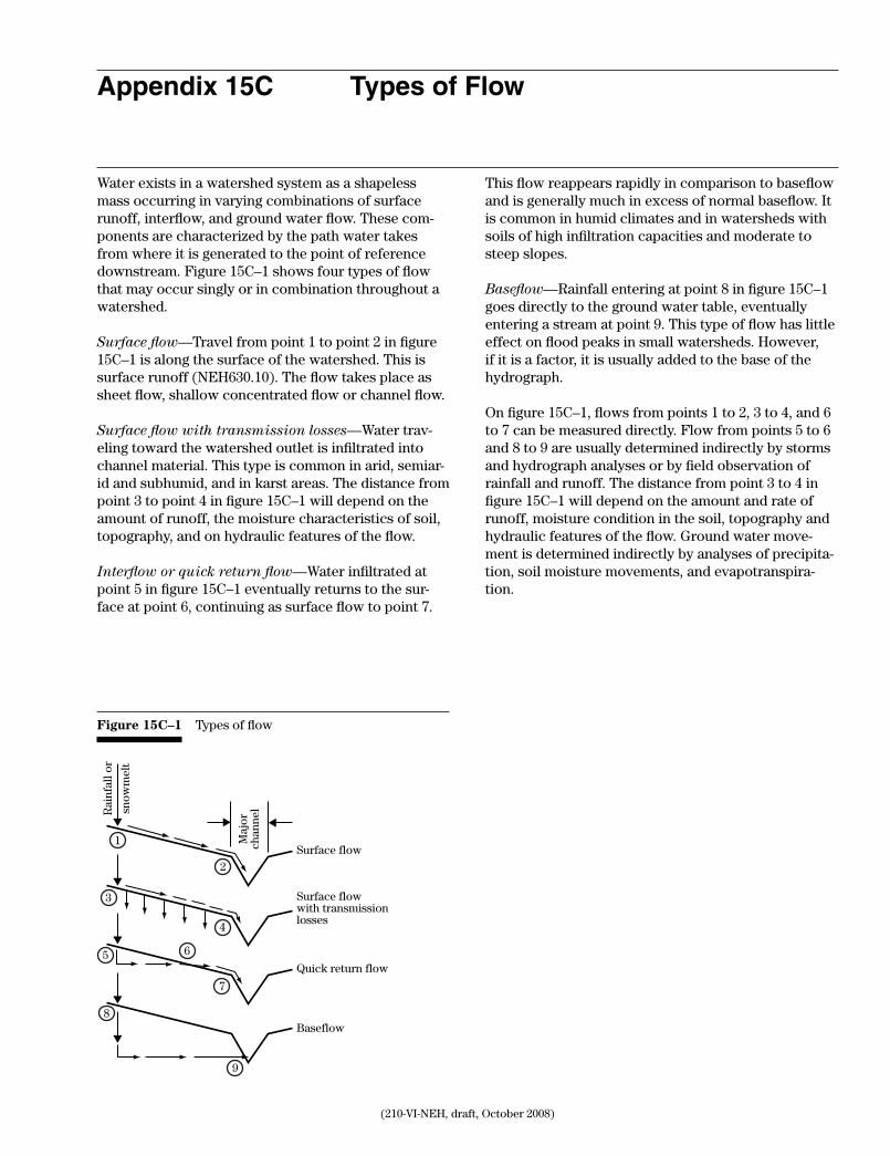
Water exists in a watershed system as a shapeless mass occurring in varying combinations of surface runoff, interflow, and ground water flow. These com-ponents are characterized by the path water takes from where it is generated to the point of reference downstream. Figure 15C–1 shows four types of flow that may occur singly or in combination throughout a watershed.

Surface flow—Travel from point 1 to point 2 in figure 15C–1 is along the surface of the watershed. This is surface runoff (NEH630.10). The flow takes place as sheet flow, shallow concentrated flow or channel flow.

Surface flow with transmission losses—Water trav-eling toward the watershed outlet is infiltrated into channel material. This type is common in arid, semiar-id and subhumid, and in karst areas. The distance from point 3 to point 4 in figure 15C–1 will depend on the amount of runoff, the moisture characteristics of soil, topography, and on hydraulic features of the flow.

Interflow or quick return flow—Water infiltrated at point 5 in figure 15C–1 eventually returns to the sur-face at point 6, continuing as surface flow to point 7.

This flow reappears rapidly in comparison to baseflow and is generally much in excess of normal baseflow. It is common in humid climates and in watersheds with soils of high infiltration capacities and moderate to steep slopes.

Baseflow—Rainfall entering at point 8 in figure 15C–1 goes directly to the ground water table, eventually entering a stream at point 9. This type of flow has little effect on flood peaks in small watersheds. However, if it is a factor, it is usually added to the base of the hydrograph.

On figure 15C–1, flows from points 1 to 2, 3 to 4, and 6 to 7 can be measured directly. Flow from points 5 to 6 and 8 to 9 are usually determined indirectly by storms and hydrograph analyses or by field observation of rainfall and runoff. The distance from point 3 to 4 in figure 15C–1 will depend on the amount and rate of runoff, moisture condition in the soil, topography and hydraulic features of the flow. Ground water move-ment is determined indirectly by analyses of precipita-tion, soil moisture movements, and evapotranspira-tion.

Appendix 15C Types of Flow

1

2

3

4

Surface flow

Maj

orch

anne

lRai

nfal

l or

snow

mel

t

Surface flowwith transmission losses

Quick return flow

Baseflow

65

7

8

9

Figure 15C–1 Types of flow

Chapter 15: Time of Concentration - Irrigation ToolBoxirrigationtoolbox.com/NEH/Part630_Hydrology/NEH630-ch15draft.pdf · Chapter 15 Time of Concentration. ... its programs and activities

Documents