Chapter 13

Chapter 13

ANTENNAS

The Ten Commandments of Success1. Hard Work: Hard work is the best investment a man can make.2. Study Hard: Knowledge enables a man to work more intelligently and effec-

tively.3. Have Initiative: Ruts often deepen into graves.4. Love Your Work: Then you will find pleasure in mastering it.5. Be Exact: Slipshod methods bring slipshod results.6. Have the Spirit of Conquest: Thus you can successfully battle and overcome

difficulties.7. Cultivate Personality: Personality is to a man what perfume is to the flower.8. Help and Share with Others: The real test of business greatness lies in giving

opportunity to others.9. Be Democratic: Unless you feel right toward your fellow men, you can never

be a successful leader of men.10. In all Things Do Your Best: The man who has done his best has done every-

thing. The man who has done less than his best has done nothing.

—CHARLES M. SCHWAB

13.1 INTRODUCTION

Up until now, we have not asked ourselves how EM waves are produced. Recall that elec-tric charges are the sources of EM fields. If the sources are time varying, EM waves prop-agate away from the sources and radiation is said to have taken place. Radiation may bethought of as the process of transmitting electric energy. The radiation or launching of thewaves into space is efficiently accomplished with the aid of conducting or dielectric struc-tures called antennas. Theoretically, any structure can radiate EM waves but not all struc-tures can serve as efficient radiation mechanisms.

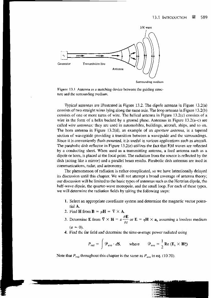
An antenna may also be viewed as a transducer used in matching the transmission lineor waveguide (used in guiding the wave to be launched) to the surrounding medium or viceversa. Figure 13.1 shows how an antenna is used to accomplish a match between the lineor guide and the medium. The antenna is needed for two main reasons: efficient radiationand matching wave impedances in order to minimize reflection. The antenna uses voltageand current from the transmission line (or the EM fields from the waveguide) to launch anEM wave into the medium. An antenna may be used for either transmitting or receivingEM energy.

588

13.1 INTRODUCTION 589

EM wave

Generator Transmission line

Antenna

Surrounding medium

Figure 13.1 Antenna as a matching device between the guiding struc-ture and the surrounding medium.

Typical antennas are illustrated in Figure 13.2. The dipole antenna in Figure 13.2(a)consists of two straight wires lying along the same axis. The loop antenna in Figure 13.2(b)consists of one or more turns of wire. The helical antenna in Figure 13.2(c) consists of awire in the form of a helix backed by a ground plane. Antennas in Figure 13.2(a-c) arecalled wire antennas; they are used in automobiles, buildings, aircraft, ships, and so on.The horn antenna in Figure 13.2(d), an example of an aperture antenna, is a taperedsection of waveguide providing a transition between a waveguide and the surroundings.Since it is conveniently flush mounted, it is useful in various applications such as aircraft.The parabolic dish reflector in Figure 13.2(e) utilizes the fact that EM waves are reflectedby a conducting sheet. When used as a transmitting antenna, a feed antenna such as adipole or horn, is placed at the focal point. The radiation from the source is reflected by thedish (acting like a mirror) and a parallel beam results. Parabolic dish antennas are used incommunications, radar, and astronomy.

The phenomenon of radiation is rather complicated, so we have intentionally delayedits discussion until this chapter. We will not attempt a broad coverage of antenna theory;our discussion will be limited to the basic types of antennas such as the Hertzian dipole, thehalf-wave dipole, the quarter-wave monopole, and the small loop. For each of these types,we will determine the radiation fields by taking the following steps:

1. Select an appropriate coordinate system and determine the magnetic vector poten-tial A.

2. Find H from B = /tH = V X A.

3. Determine E from V X H = e or E = i;H X as assuming a lossless mediumdt

(a = 0).4. Find the far field and determine the time-average power radiated using

dS, where ve = | Re (E, X H*)

Note that Pnd throughout this chapter is the same as Pme in eq. (10.70).

590 Antennas

(a) dipole (b) loop

(c) helix

(d) pyramidal horn

Radiatingdipole

Reflector

(e) parabolic dish reflector

Figure 13.2 Typical antennas.

13.2 HERTZIAN DIPOLE

By a Hertzian dipole, we mean an infinitesimal current element / dl. Although such acurrent element does not exist in real life, it serves as a building block from which the fieldof a practical antenna can be calculated by integration.

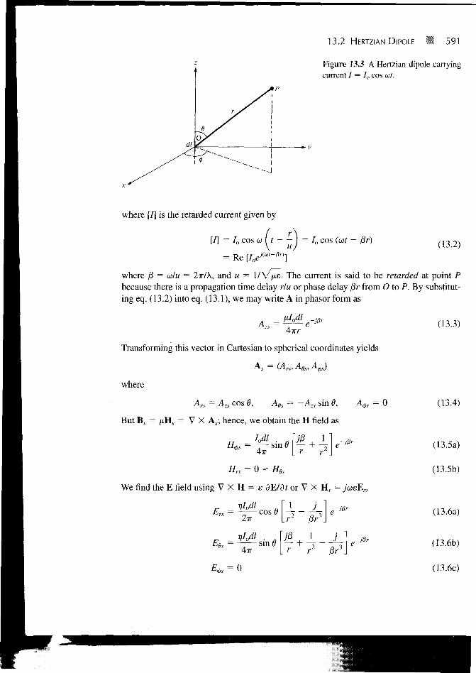
Consider the Hertzian dipole shown in Figure 13.3. We assume that it is located at theorigin of a coordinate system and that it carries a uniform current (constant throughout thedipole), I = Io cos cot. From eq. (9.54), the retarded magnetic vector potential at the fieldpoint P, due to the dipole, is given by

A =A-wr

(13.1)

13.2 HERTZIAN DIPOLE 591

Figure 13.3 A Hertzian dipole carryingcurrent I = Io cos cot.

where [/] is the retarded current given by

[/] = Io cos a) ( t ) = Io cos {bit - (3r)u J

(13.2)= Re [Ioe

j(M-M]

where (3 = to/w = 2TT/A, and u = 1/V/xe. The current is said to be retarded at point Pbecause there is a propagation time delay rlu or phase delay /3r from O to P. By substitut-ing eq. (13.2) into eq. (13.1), we may write A in phasor form as

(13.3)Azs A e

Transforming this vector in Cartesian to spherical coordinates yields

A, = (Ars, A6s, A^)

where

A n . = A z s cos 8, Affs = —Azs sin 6,

But B, = ^H, = V X As; hence, we obtain the H field as

= 0

IodlH^ = —— sin 0 — + - r e

j!3

** 4x lr r-

Hrs = 0 = //Ss

We find the E field using V X H = e dWdt or V X Hs = jueEs,

_ : , - u — ^ ^ fl ! _ - j__ | ^ - 7 / 3 r

E^ = 0

r r

(13.4)

(13.5a)

(13.5b)

(13.6a)

(13.6b)

(13.6c)

592 Hi Antennas

where

V =

A close observation of the field equations in eqs. (13.5) and (13.6) reveals that wehave terms varying as 1/r3, 1/r2, and 1/r. The 1/r3 term is called the electrostatic field sinceit corresponds to the field of an electric dipole [see eq. (4.82)]. This term dominates overother terms in a region very close to the Hertzian dipole. The 1/r term is called the induc-tive field, and it is predictable from the Biot-Savart law [see eq. 7.3)]. The term is impor-tant only at near field, that is, at distances close to the current element. The 1/r term iscalled the far field or radiation field because it is the only term that remains at the far zone,that is, at a point very far from the current element. Here, we are mainly concerned with thefar field or radiation zone (j3r 5> 1 or 2irr S> X), where the terms in 1/r3 and 1/r2 can beneglected in favor of the 1/r term. Thus at far field,

4-irrsin 6 e - V

- Ers - = 0

(I3.7a)

(I3.7b)

Note from eq. (13.7a) that the radiation terms of H$s and E9s are in time phase and orthog-onal just as the fields of a uniform plane wave. Also note that near-zone and far-zone fieldsare determined respectively to be the inequalities /3r <$C I and f3r > I. More specifically,we define the boundary between the near and the far zones by the value of r given by

2d2

r = (13.8)

where d is the largest dimension of the antenna.The time-average power density is obtained as

12Pave = ~ Re (Es X H*) = ^ Re (E6s H% ar)

(13.9)

Substituting eq. (13.7) into eq. (13.9) yields the time-average radiated power as

dS

<t>=o Je=o

3 2 T T 2

327r2r2sin2 6 r2 sin 6 dd d<j> (13.10)

2TT sin* 6 dO

13.2 HERTZIAN DIPOLE • 593

But

sin' 6d6 = \ (1 - cosz 0) d(-cos 9)

cos30— cos i

and 02 = 4TT2/X2. Hence eq. (13.10) becomes

^rad ~dl

3 L X.

If free space is the medium of propagation, rj = 120TT and

(13.11a)

(13.11b)

This power is equivalent to the power dissipated in a fictitious resistance /?rad by currentI = Io cos cot that is

~rad * rms " rad

or

1(13.12)

where /rms is the root-mean-square value of/. From eqs. (13.11) and (13.12), we obtain

OPr» z ' * rad /1 o 11 \

rad = -ZV (13.13a)

or

(13.13b)

The resistance Rmd is a characteristic property of the Hertzian dipole antenna and is calledits radiation resistance. From eqs. (13.12) and (13.13), we observe that it requires anten-nas with large radiation resistances to deliver large amounts of power to space. Forexample, if dl = X/20, Rrad = 2 U, which is small in that it can deliver relatively smallamounts of power. It should be noted that /?rad in eq. (13.13b) is for a Hertzian dipole infree space. If the dipole is in a different, lossless medium, rj = V/x/e is substituted ineq. (13.11a) and /?rad is determined using eq. (13.13a).

Note that the Hertzian dipole is assumed to be infinitesimally small (& dl <S^ 1 ordl ^ X/10). Consequently, its radiation resistance is very small and it is in practice difficultto match it with a real transmission line. We have also assumed that the dipole has a

594 Antennas

uniform current; this requires that the current be nonzero at the end points of the dipole.This is practically impossible because the surrounding medium is not conducting.However, our analysis will serve as a useful, valid approximation for an antenna withdl s X/10. A more practical (and perhaps the most important) antenna is the half-wavedipole considered in the next section.

13.3 HALF-WAVE DIPOLE ANTENNA

The half-wave dipole derives its name from the fact that its length is half a wavelength(€ = A/2). As shown in Figure 13.4(a), it consists of a thin wire fed or excited at the mid-point by a voltage source connected to the antenna via a transmission line (e.g., a two-wireline). The field due to the dipole can be easily obtained if we consider it as consisting of achain of Hertzian dipoles. The magnetic vector potential at P due to a differential lengthdl(= dz) of the dipole carrying a phasor current Is = Io cos fiz is

(13.14)

Transmissionline

Dipoleantenna

Current distribution Figure 13.4 A half-wave dipole./ = /„ cos /3z

t' \

(a)

13.3 HALF-WAVE DIPOLE ANTENNA 595

Notice that to obtain eq. (13.14), we have assumed a sinusoidal current distributionbecause the current must vanish at the ends of the dipole; a triangular current distributionis also possible (see Problem 13.4) but would give less accurate results. The actual currentdistribution on the antenna is not precisely known. It is determined by solving Maxwell'sequations subject to the boundary conditions on the antenna, but the procedure is mathe-matically complex. However, the sinusoidal current assumption approximates the distribu-tion obtained by solving the boundary-value problem and is commonly used in antenna

theory.If r S> €, as explained in Section 4.9 on electric dipoles (see Figure 4.21), then

r - r' = z cos i or

Thus we may substitute r' — r in the denominator of eq. (13.14) where the magnitudeof the distance is needed. For the phase term in the numerator of eq. (13.14), the dif-ference between fir and ftr' is significant, so we replace r' by r — z cos 6 and not r. Inother words, we maintain the cosine term in the exponent while neglecting it in the de-nominator because the exponent involves the phase constant while the denominator doesnot. Thus,

-W4

4irr

A/4(13.15)

j8z cos e cos fiz dz- A / 4

From the integral tables of Appendix A.8,

eaz cos bz dz =eaz {a cos bz + b sin bz)

Applying this to eq. (13.15) gives

Azs =

nloe~jl3rejl3zcose UP cos 0 cos (3z + ff sin ffz)A/4

- A / 4

(13.16)

Since 0 = 2x/X or (3 X/4 = TT/2 and -cos2 0 + 1 = sin2 0, eq. (13.16) becomes

A,, = - ^ " f ' \ [e^n)™\0 + 13)- e -^«)«»» ( 0 _ ft] ( 1 3 - 1 7 )

A-wrfi sin 0

Using the identity eJX + e~;;c = 2 cos x, we obtain

\- cos 6> )

(13.18)txloe

i&rcos I - c o s I

2Trrj3sin2 6

596 • Antennas

We use eq. (13.4) in conjunction with the fact that B^ = /*HS = V X As and V X H , =y'coeEs to obtain the magnetic and electric fields at far zone (discarding the 1/r3 and 1/r2

terms) as

(13.19)

Notice again that the radiation term of H^,s and E$s are in time phase and orthogonal.Using eqs. (13.9) and (13.19), we obtain the time-average power density as

cos2 ( — cos 6 (13.20)

8TTV sin2 $

The time-average radiated power can be determined as

2 COS22-K fw I ? / 2 COS2 I ^ COS

= 0 8x2r2 sin2 $r2 sin 0 d6 d<j>

2TT

(13.21)

sin i

JrT COS I — COS I

^-s—~d e

o sm0

where t\ = 120TT has been substituted assuming free space as the medium of propagation.Due to the nature of the integrand in eq. (13.21),

TT/2 COS - COS 6

sine

cos~l — cos I

de= I — — '-desin 0J0 "'" " Jitl2

This is easily illustrated by a rough sketch of the variation of the integrand with d. Hence

= 60/2

IT- c o s i

sin I(13.22)

13.3 HALF-WAVE DIPOLE ANTENNA S 597

Changing variables, u = cos 6, and using partial fraction reduces eq. (13.22) to

C O S 2 - T T

\-u2 du

= 307'

2 1 2 1COS —KU r , COS ~KU

2 2 j

du + \ — du1 + U 01 - u

(13.23)

Replacing 1 + u with v in the first integrand and 1 — u with v in the second results in

rad = 30/2,

= 30/2

, sin2—7TV

dv +L'0

2 S in 2 -7TV

2 sin -TTV

dv

(13.24)

Changing variables, w = irv, yields

2TT sin — w- dw

= 15/

= 15 / '

2 [ ^ (1 — COS

2! 4! 6! 8!

(13.25)

w2 w4 w6 w8

since cos w = l H 1 • •. Integrating eq. (13.25) term by term and2! 4! 6! 8!

evaluating at the limit leads to

2 f (2TT)2 (2TT)4 (2?r)6 (2TT)8

~ 1 5 / ° L 2(2!) ~ 4(4!) + 6(6!) ~ 8(8!)

= 36.56 ll

+ (13.26)

The radiation resistance Rrad for the half-wave dipole antenna is readily obtained fromeqs. (13.12) and (13.26) as

(13.27)

598 Antennas

Note the significant increase in the radiation resistance of the half-wave dipole over that ofthe Hertzian dipole. Thus the half-wave dipole is capable of delivering greater amounts ofpower to space than the Hertzian dipole.

The total input impedance Zin of the antenna is the impedance seen at the terminals ofthe antenna and is given by

~ "in (13.28)

where Rin = Rmd for lossless antenna. Deriving the value of the reactance Zin involves acomplicated procedure beyond the scope of this text. It is found that Xin = 42.5 0, soZin = 73 + y'42.5 0 for a dipole length £ = X/2. The inductive reactance drops rapidly tozero as the length of the dipole is slightly reduced. For € = 0.485 X, the dipole is resonant,with Xin = 0. Thus in practice, a X/2 dipole is designed such that Xin approaches zero andZin ~ 73 0. This value of the radiation resistance of the X/2 dipole antenna is the reason forthe standard 75-0 coaxial cable. Also, the value is easy to match to transmission lines.These factors in addition to the resonance property are the reasons for the dipole antenna'spopularity and its extensive use.

13.4 QUARTER-WAVE MONOPOLE ANTENNA

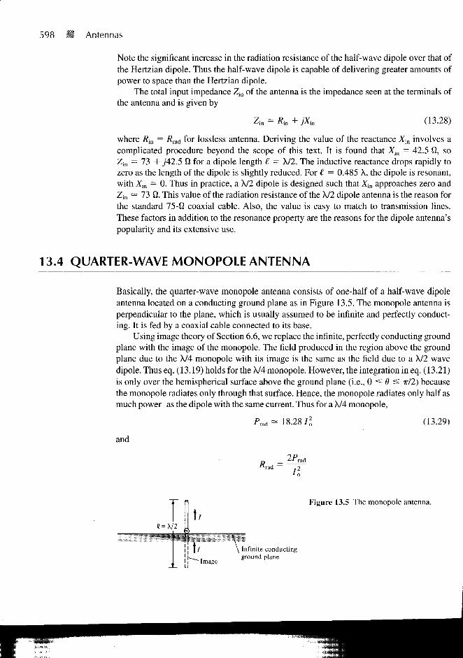
Basically, the quarter-wave monopole antenna consists of one-half of a half-wave dipoleantenna located on a conducting ground plane as in Figure 13.5. The monopole antenna isperpendicular to the plane, which is usually assumed to be infinite and perfectly conduct-ing. It is fed by a coaxial cable connected to its base.

Using image theory of Section 6.6, we replace the infinite, perfectly conducting groundplane with the image of the monopole. The field produced in the region above the groundplane due to the X/4 monopole with its image is the same as the field due to a X/2 wavedipole. Thus eq. (13.19) holds for the X/4 monopole. However, the integration in eq. (13.21)is only over the hemispherical surface above the ground plane (i.e., 0 < d < TT/2) becausethe monopole radiates only through that surface. Hence, the monopole radiates only half asmuch power as the dipole with the same current. Thus for a X/4 monopole,

- 18.28/2 (13.29)

and

IP ad

Figure 13.5 The monopole antenna.

"Image

^ Infinite conductingground plane

13.5 SMALL LOOP ANTENNA 599

or

Rmd = 36.5 0 (13.30)

By the same token, the total input impedance for a A/4 monopole is Zin = 36.5 + _/21.25 12.

13.5 SMALL LOOP ANTENNA

The loop antenna is of practical importance. It is used as a directional finder (or searchloop) in radiation detection and as a TV antenna for ultrahigh frequencies. The term"small" implies that the dimensions (such as po) of the loop are much smaller than X.

Consider a small filamentary circular loop of radius po carrying a uniform current,Io cos co?, as in Figure 13.6. The loop may be regarded as an elemental magnetic dipole.The magnetic vector potential at the field point P due to the loop is

A =/*[/]</! (13.31)

where [7] = 7O cos (cor - /3r') = Re [loeji"' ISr)]. Substituting [7] into eq. (13.31), we

obtain A in phasor form as

e~jfir'e

Ait ]L r'(13.32)

Evaluating this integral requires a lengthy procedure. It can be shown that for a small loop(po <SC \ ) , r' can be replaced by r in the denominator of eq. (13.32) and As has only <f>-component given by

^<*sA-K?

(1 + j$r)e~i&r sin 6 (13.33)

Figure 13.6 The small loop antenna.

N Transmiss ion line

600 Antennas

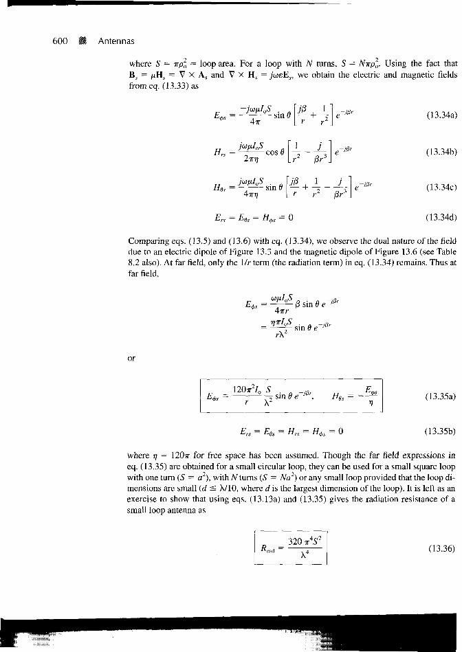
where S = wpl = loop area. For a loop with N turns, S = Nirpl. Using the fact thatBs = /xHs = VX A, and V X H S = ju>sEs, we obtain the electric and magnetic fieldsfrom eq. (13.33) as

Ai:sin I (13.34a)

2m,

4TTT/

/3r3

sin 0 J— + - r -2 )3rJ

ra - Eds - H<f>s - 0

(13.34b)

(13.34c)

(13.34d)

Comparing eqs. (13.5) and (13.6) with eq. (13.34), we observe the dual nature of the fielddue to an electric dipole of Figure 13.3 and the magnetic dipole of Figure 13.6 (see Table8.2 also). At far field, only the 1/r term (the radiation term) in eq. (13.34) remains. Thus atfar field,

4irr18 sin 6 e

r\2 sin o e

or

(13.35a)

- Hrs - - 0 (13.35b)

where 77 = 120TT for free space has been assumed. Though the far field expressions ineq. (13.35) are obtained for a small circular loop, they can be used for a small square loopwith one turn (S = a ) , with Af turns (S = Na2) or any small loop provided that the loop di-mensions are small (d < A/10, where d is the largest dimension of the loop). It is left as anexercise to show that using eqs. (13.13a) and (13.35) gives the radiation resistance of asmall loop antenna as

(13.36)

13.5 SMALL LOOP ANTENNA M 601

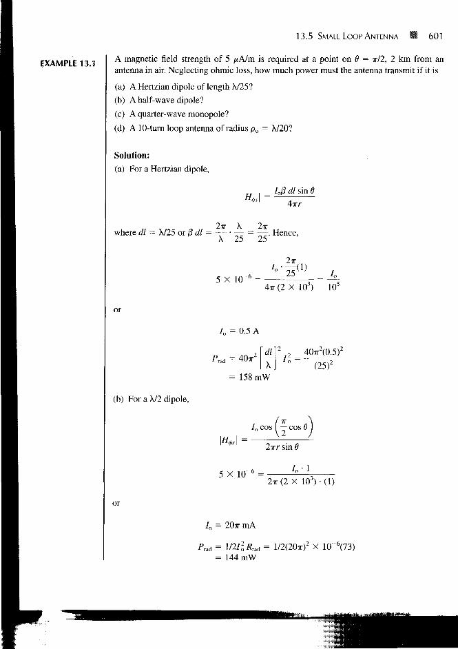
EXAMPLE 13.1 A magnetic field strength of 5 ^A/m is required at a point on 6 = TT/2, 2 km from anantenna in air. Neglecting ohmic loss, how much power must the antenna transmit if it is

(a) A Hertzian dipole of length X/25?

(b) A half-wave dipole?

(c) A quarter-wave monopole?

(d) A 10-turn loop antenna of radius po = X/20?

Solution:

(a) For a Hertzian dipole,

_ 7o/3 dl sin 6051 A

4irr

where dl = X/25 or 0 dl = = —. Hence,

5 X 1(T6 =4TT (2 X 103) 105

or

Io = 0.5 A

'™H = 40TT2 I ^X

= 158 mW

40x2(0.5)2

(25)2

(b) For a X/2 dipole,

5 x

/o cos I — cos

2irr sin 6

/„ • 12TT(2 X

or

/„ = 207T mA

/^/? rad = 1/2(20TT)Z X 10~°(73)= 144 mW

602 B Antennas

(c) For a X/4 monopole,

as in part (b).

(d) For a loop antenna,

2

/ o = 20TT mA

= l/2I20Rmd = 1/2(20TT)2 X 10~6(36.56)

= 72 mW

*• /„ S .

r X2sin 8

For a single turn, S = •Kpo. For ,/V-turn, S = N-wp0. Hence,

or

5 X io - 6 = ^ ^ - ^2 X 103 L X

10

IOTT2 LPO

= 40.53 mA

— I X 10"3 =

= 320 7T6 X 100 iol =192-3fi

Z'rad = ^/o^rad = ~ (40.53)2 X 10"6 (192.3)

= 158 mW

PRACTICE EXERCISE 13.1

A Hertzian dipole of length X/100 is located at the origin and fed with a current of0.25 sin 108f A. Determine the magnetic field at

(a) r = X/5,0 = 30°

(b) r = 200X, 6 = 60°

Answer: (a) 0.2119 sin (10s? - 20.5°) a0 mA/m, (b) 0.2871 sin (l08t + 90°) a0

13.5 SMALL LOOP ANTENNA 603

EXAMPLE 13.2An electric field strength of 10 /uV/m is to be measured at an observation point 6 = ir/2,500 km from a half-wave (resonant) dipole antenna operating in air at 50 MHz.

(a) What is the length of the dipole?

(b) Calculate the current that must be fed to the antenna.

(c) Find the average power radiated by the antenna.

(d) If a transmission line with Zo = 75 0 is connected to the antenna, determine the stand-ing wave ratio.

Solution:

c 3 X 108

(a) The wavelength X = - = r = 6 m./ 50 X 106

Hence, the length of the half-dipole is € = — = 3 m.

(b) From eq. (13.19),

r)Jo cos ( — cos 6

2-wr sin 6

or

2irr sin 9

r)o cos I — cos 6\2 j

10 X 10" 6 2TT(500 X 103) • (1)

120ir(l)

(c)

= 83.33 mA

Rmd = 73 Q

= \ (83.33)2 X 10-6 X 73

(d)

= 253.5 mW

F = — - (ZL = Zin in this case)z,£ + Zo

73 + y'42.5 - 75 _ - 2 + y'42.573 + y"42.5 + 75 ~42.55/92.69°

153.98/16.02

148 + y'42.5

= 0.2763/76.67°

s =1 + | r | 1 + 0.2763

- r 1 - 0.2763= 1.763

604 Antennas

PRACTICE EXERCISE 13.2

Repeat Example 13.2 if the dipole antenna is replaced by a X/4 monopole.

Answer: (a) 1.5m, (b) 83.33 mA, (c) 126.8 mW, (d) 2.265.

13.6 ANTENNA CHARACTERISTICS

Having considered the basic elementary antenna types, we now discuss some importantcharacteristics of an antenna as a radiator of electromagnetic energy. These characteristicsinclude: (a) antenna pattern, (b) radiation intensity, (c) directive gain, (d) power gain.

A. Antenna Patterns

An antenna pattern (or radiation pattern) is a ihrce-climensional plot of iis radia-tion ai fur field.

When the amplitude of a specified component of the E field is plotted, it is called the fieldpattern or voltage pattern. When the square of the amplitude of E is plotted, it is called thepower pattern. A three-dimensional plot of an antenna pattern is avoided by plotting sepa-rately the normalized \ES\ versus 0 for a constant 4> (this is called an E-plane pattern or ver-tical pattern) and the normalized \ES\ versus <t> for 8 = TT/2 (called the H-planepattern orhorizontal pattern). The normalization of \ES\ is with respect to the maximum value of the

so that the maximum value of the normalized \ES\ is unity.For the Hertzian dipole, for example, the normalized |iSj| is obtained from eq. (13.7) as

= |sin0| (13.37)

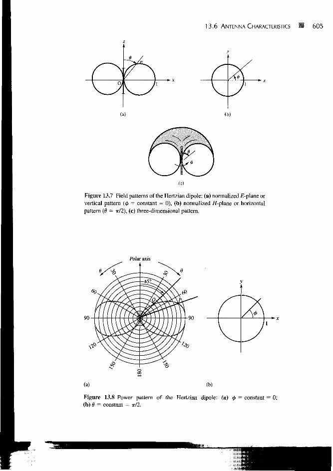
which is independent of <t>. From eq. (13.37), we obtain the £-plane pattern as the polarplot of j{8) with 8 varying from 0° to 180°. The result is shown in Figure 13.7(a). Note thatthe plot is symmetric about the z-axis (8 = 0). For the /f-plane pattern, we set 8 = TT/2 SOthat/(0) = 1, which is circle of radius 1 as shown in Figure 13.7(b). When the two plots ofFigures 13.7(a) and (b) are combined, we have a three-dimensional field pattern of Figure13.7(c), which has the shape of a doughnut.

A plot of the time-average power, |2Pave| = 2Pave, for a fixed distance r is the powerpattern of the antenna. It is obtained by plotting separately 2Pave versus 8 for constant <j> andS ave versus 4> for constant 8.

For the Hertzian dipole, the normalized power pattern is easily obtained from eqs.(13.37) or (13.9) as

/2(0) = sin2 0 (13.38)

which is sketched in Figure 13.8. Notice that Figures 13.7(b) and 13.8(b) show circlesbecause fi8) is independent of <j> and that the value of OP in Figure 13.8(a) is the relative

13.6 ANTENNA CHARACTERISTICS B 605

(a)

(c)

Figure 13.7 Field patterns of the Hertzian dipole: (a) normalized £-plane orvertical pattern (4> = constant = 0), (b) normalized ff-plane or horizontalpattern (6 = TT/2), (C) three-dimensional pattern.

Polar axis

(a) (b)

Figure 13.8 Power pattern of the Hertzian dipole: (a) 4> = constant = 0;(b) 6 = constant = T/2.

606 Antennas

average power for that particular 6. Thus, at point Q (0 = 45°), the average power is one-half the maximum average power (the maximum average power is at 6 = TT/2).

B. Radiation Intensity

The radiation intensity of an antenna is defined as

me, 0) = r2 g>a. (13.39)

From eq. (13.39), the total average power radiated can be expressed as

Sin 6 dd d$

= U{d,<j>) sin dd$d<t> (13.40)

2ir fir

U(6, </>) dU•=o Je=o

where dQ = sin 9 dd d(f> is the differential solid angle in steradian (sr). Hence the radiationintensity U(6, <f>) is measured in watts per steradian (W/sr). The average value of U(d, <j>) isthe total radiated power divided by 4TT sr; that is,

rrad

4?T(13.41)

C. Directive Gain

Besides the antenna patterns described above, we are often interested in measurable quan-tities such as gain and directivity to determine the radiation characteristics of an antenna.

The directive gain (i/0.6) of itn unlenna is a measure of the concentration of the ra-diated power in a particular direction (e. <p).

It may be regarded as the ability of the antenna to direct radiated power in a given direc-tion. It is usually obtained as the ratio of radiation intensity in a given direction (6, <f>) to theaverage radiation intensity, that is

(13.42)

13.6 ANTENNA CHARACTERISTICS 607

By substituting eq. (13.39) into eq. (13.42), 0 ^ may be expressed in terms of directivegain as

(13.43)=ave . ?

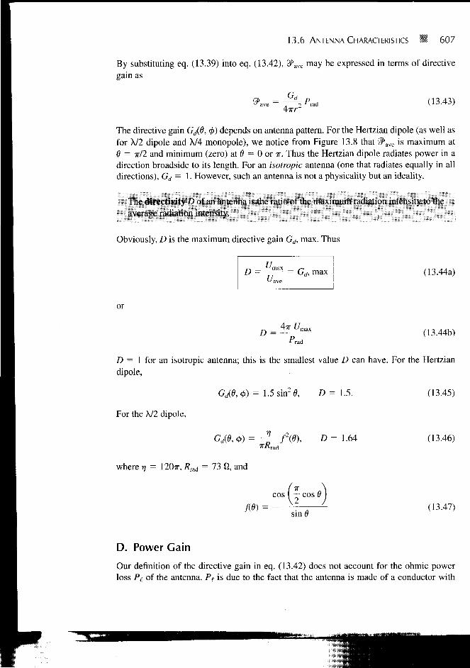
AirrThe directive gain GJfi, <j>) depends on antenna pattern. For the Hertzian dipole (as well asfor A/2 dipole and X/4 monopole), we notice from Figure 13.8 that 2Pave is maximum at6 = 7r/2 and minimum (zero) at 6 = 0 or TT. Thus the Hertzian dipole radiates power in adirection broadside to its length. For an isotropic antenna (one that radiates equally in alldirections), Gd = 1. However, such an antenna is not a physicality but an ideality.

The directivity I) of an antenna is ihe ratio of the maximum radiation intensity to theaverage radiaiion intensity.

Obviously, D is the maximum directive gain Gd, max. Thus

D = —— = Gd, max (13.44a)

or

D =•Prad

(13.44b)

D = 1 for an isotropic antenna; this is the smallest value D can have. For the Hertziandipole,

G/6,<j)) = 1.5 sin2 0, D = 1.5.

For the A/2 dipole,

(13.45)

Gd(d, </>) =

where i\ = 120x, /?rad = 73 fi, and

), D=\Mrad

ITCOS | — COS I

sin0

(13.46)

(13.47)

D. Power Gain

Our definition of the directive gain in eq. (13.42) does not account for the ohmic powerloss P( of the antenna. Pt is due to the fact that the antenna is made of a conductor with

608 Antennas

finite conductivity. As illustrated in Figure 13.9, if Pin is the total input power to theantenna,

Pin — +

+(13.48)

where 7in is the current at the input terminals and R( is the loss or ohmic resistance of theantenna. In other words, Pin is the power accepted by the antenna at its terminals during theradiation process, and Prad is the power radiated by the antenna; the difference between thetwo powers is P(, the power dissipated within the antenna.

We define the power gain Gp(6, <j>) of the antenna as

(13.49)

The ratio of the power gain in any specified direction to the directive gain in that directionis referred to as the radiation efficiency v\r of the antennas, that is

GPVr =

Introducing eq. (13.48) leads to

Vr =Pr,ad Vad

Rf(13.50)

For many antennas, r\r is close to 100% so that GP — Gd. It is customary to express direc-tivity and gain in decibels (dB). Thus

D(dB) = 101og,0£»

G (dB) = 10 log10 G

(13.51a)

(13.51b)

It should be mentioned at this point that the radiation patterns of an antenna areusually measured in the far field region. The far field region of an antenna is commonlytaken to exist at distance r > rmin where

2dz

(13.52)

Figure 13.9 Relating P-m, P(, and Prad.

Prad

13.6 ANTENNA CHARACTERISTICS 609

and d is the largest dimension of the antenna. For example, d = I for the electric dipoleantenna and d = 2p0 for the small loop antenna.

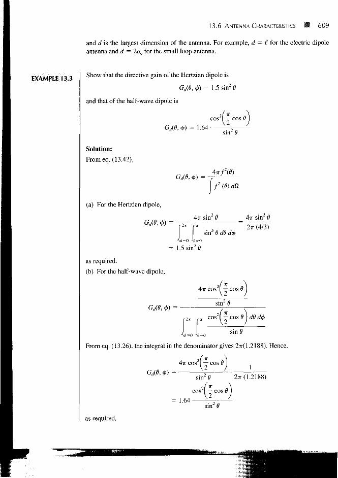
EXAMPLE 13.3 Show that the directive gain of the Hertzian dipole is

Gd(0, <£) = 1.5 sin2 6

and that of the half-wave dipole is

cos ( — cos 6Gd(9,<t>) = 1 - 6 4 —

sin (

Solution:

From eq. (13.42),

, <f>) =4TT/2(0)

f (6) d

(a) For the Hertzian dipole,

4TT sin2 6

sin3 6 d6 d<j)

4TT sin2 6

2TT (4/3)

= 1.5 sin2 6

as required.

(b) For the half-wave dipole,

4TT COS — cos

sin2

2lr rir cos I — cos 6 I dO d(f>

G/.9, <t>) =

From eq. (13.26), the integral in the denominator gives 27r(1.2188). Hence,

G/.8, 0) =4TT cos2! — cos 9

sin20 (1.2188)

= 1.64cos I — cos I

sin20

as required.

610 Antennas

PRACTICE EXERCISE 13.3

Calculate the directivity of

(a) The Hertzian monopole

(b) The quarter-wave monopole

Answer: (a) 3, (b) 3.28.

EXAMPLE 13.4 Determine the electric field intensity at a distance of 10 km from an antenna having a di-rective gain of 5 dB and radiating a total power of 20 kW.

Solution:

or

From eq. (13.43),

But

Hence,

5 = Gd(dB) = 101og10Grf

0.5 = log10 Gd -

GdPrad

= lO05 = 3.162

at, =u ave

op =° ave

4-irr

\E,2V

1207T(3.162)(20 X 103)E = =

2irr2 2TT[10 X 103]2

Es\ = 0.1948 V/m

PRACTICE EXERCISE 13.4

A certain antenna with an efficiency of 95% has maximum radiation intensity of0.5 W/sr. Calculate its directivity when

(a) The input power is 0.4 W

(b) The radiated power is 0.3 W

Answer: (a) 16.53, (b) 20.94.

EXAMPLE 13.5

13.6 ANTENNA CHARACTERISTICS

The radiation intensity of a certain antenna is

2 sin d sin3 0, 0 < 0 < TT, 0 < 0 < TT

611

U(8, 0) =0, elsewhere

Determine the directivity of the antenna.

Solution:

The directivity is defined as

D =ua.

From the given U,

= 2

_ _1_

1

~ 4TT

_ J_~ 2TT

9 «i=o •/e=o

s in 0 s in <j> s in 0 d<j>

s i n ' <j>d<t>o

= ^ - - (1 - cos 20) d0 (1 - cosz 0) rf(-cos (A)27r 4 2 4sin

2TT2

27r\2j\3j 3

/ COS (f)I cos io l 3

Hence

Z) =(1/3)

— 6

PRACTICE EXERCISE 13.5

Evaluate the directivity of an antenna with normalized radiation intensity

fsin 0, 0 < 0 < TT/2, 0 < 0 < 2TT[0, otherwise

Answer: 2.546.

612 B Antennas

13.7 ANTENNA ARRAYS

In many practical applications (e.g., in an AM broadcast station), it is necessary to designantennas with more energy radiated in some particular directions and less in other direc-tions. This is tantamount to requiring that the radiation pattern be concentrated in the di-rection of interest. This is hardly achievable with a single antenna element. An antennaarray is used to obtain greater directivity than can be obtained with a single antennaelement.

An antenna array is a group of radiating elements arranged so us to produce someparticular radiation characteristics.

It is practical and convenient that the array consists of identical elements but this isnot fundamentally required. We shall consider the simplest case of a two-elementarray and extend our results to the more complicated, general case of an N-elementarray.

Consider an antenna consisting of two Hertzian dipoles placed in free space along thez-axis but oriented parallel to the ;t-axis as depicted in Figure 13.10. We assume that thedipole at (0, 0, d/2) carries current Ils = I0/cx and the one at (0, 0, -d/2) carries currenths = 4 / 0 . where a is the phase difference between the two currents. By varying thespacing d and phase difference a, the fields from the array can be made to interfere con-structively (add) in certain directions of interest and interfere destructively (cancel) inother directions. The total electric field at point P is the vector sum of the fields due to theindividual elements. If P is in the far field zone, we obtain the total electric field at P fromeq. (13.7a) as

-'Is

COS0-,(13.53)

Note that sin 6 in eq. (13.7a) has been replaced by cos 6 since the element of Figure 13.3 isz-directed whereas those in Figure 13.10 are x-directed. Since P is far from the array,

Figure 13.10 A two-element array.

#i — 9 — 62 and ae< — ae

we use

13.7 ANTENNA ARRAYS S§ 613

i. In the amplitude, we can set rx — r = r2 but in the phase,

drx — r cos I

r2 — r + r cos i

(13.54a)

(13.54b)

Thus eq. (13.53) becomes

4x r->a/2j

4?r r cos cos \-L2

cos

(13.55)

Comparing this with eq. (13.7a) shows that the total field of an array is equal to the field ofsingle element located at the origin multiplied by an array factor given by

AF = 2 cos | - (/tacos 8 + u)\ eja/2 (13.56)

Thus, in general, the far field due to a two-element array is given by

E (total) = (E due to single element at origin) X (array factor) (13.57)

Also, from eq. (13.55), note that |cos d\ is the radiation pattern due to a single elementwhereas the normalized array factor, |cos[l/2(|8Jcos 6 + a)]\, is the radiation pattern ofthe array if the elements were isotropic. These may be regarded as "unit pattern" and"group pattern," respectively. Thus the "resultant pattern" is the product of the unit patternand the group pattern, that is,

Resultant pattern = Unit pattern X Group pattern (13.58)

This is known as pattern multiplication. It is possible to sketch, almost by inspection, thepattern of an array by pattern multiplication. It is, therefore, a useful tool in the design ofan array. We should note that while the unit pattern depends on the type of elements thearray is comprised of, the group pattern is independent of the element type so long as thespacing d and phase difference a, and the orientation of the elements remain the same.

Let us now extend the results on the two-element array to the general case of an N-element array shown in Figure 13.11. We assume that the array is linear in that the ele-ments are spaced equally along a straight line and lie along the z-axis. Also, we assume thatthe array is uniform so that each element is fed with current of the same magnitude but ofprogressive phase shift a, that is, Ils = /O//0,12s = Io/u, I3s = 7o/2q, and so on. We aremainly interested in finding the array factor; the far field can easily be found from eq.

614 Antennas

Figure 13.11 An iV-element uniform linear array.

- d cos 6

(13.57) once the array factor is known. For the uniform linear array, the array factor is thesum of the contributions by all the elements. Thus,

AF = 1 + eJ4r + ej2>p + + eAN-1)4,

where

= (3d cos 6 + a

(13.59)

(13.60)

In eq. (13.60), fi = 2x/X, d and a are, respectively, the spacing and interelement phaseshift. Notice that the right-hand side of eq. (13.59) is a geometric series of the form

1 + x + x2 + x3

Hence eq. (13.59) becomes

1 - x

AF =1 -

(13.61)

(13.62)

which can be written as

AF =_ e-jN4,/2

sin (Aty/2)

sin (\l//2)

(13.63)

The phase factor eJ(N l)*n would not be present if the array were centered about the origin.Neglecting this unimportant term,

(13.64)AF = \b = fid cos 6 + a

13.7 ANTENNA ARRAYS 615

Note that this equation reduces to eq. (13.56) when N = las, expected. Also, note the fol-lowing:

1. AF has the maximum value of TV; thus the normalized AF is obtained by dividingAF by N. The principal maximum occurs when \J/ = 0, that is

0 = fid cos 6 + a or

2. AF has nulls (or zeros) when AF = 0, that is

Nip

cos 0 = — a

Yd

—- = ±/br, k= 1,2, 3 , . . .

(13.65)

(13.66)

where k is not a multiple of N.3. A broadside array has its maximum radiation directed normal to the axis of the

array, that is, \p = 0, $ = 90° so that a = 0.4. An end-fire array has its maximum radiation directed along the axis of the array,

that is, \p = 0, B = so that a =

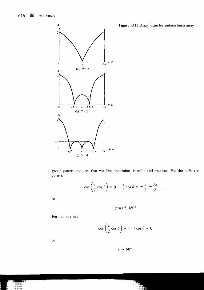
These points are helpful in plotting AF. For N=2,3, and 4, the plots of AF aresketched in Figure 13.12.

EXAMPLE 13.6 For the two-element antenna array of Figure 13.10, sketch the normalized field patternwhen the currents are:

(a) Fed in phase (a = 0), d = A/2

(b) Fed 90° out of phase (a = TT/2), d = A/4

Solution:

The normalized field of the array is obtained from eqs. (13.55) to (13.57) as

cos 6 cos - (0d cos 8 + a)

(a) If a = 0, d = A/2,13d = - ^ - = TT. Hence,A 2

1resultantpattern

= |cos0|

1= unit X

pattern

cos — (cos 6)

1grouppattern

The sketch of the unit pattern is straightforward. It is merely a rotated version of thatin Figure 13.7(a) for the Hertzian dipole and is shown in Figure 13.13(a). To sketch a

616 m Antennas

0 TT/2 IT 3TT/2 2TT

Figure 13.12 Array factor for uniform linear array.

1.08 T-V^S.—

group pattern requires that we first determine its nulls and maxima. For the nulls (orzeros),

(-K \ i „ IT 3fcos — cos 0 = 0 -»— cos 0 = ± —, ± — , . . .

\2 ) 2 2 2

or

For the maxima,

or

0 = 0°, 180°

cos ( — cos 0 ) = 1 —» cos 0 = 0

0 = 90°

unit pattern(a)

x X

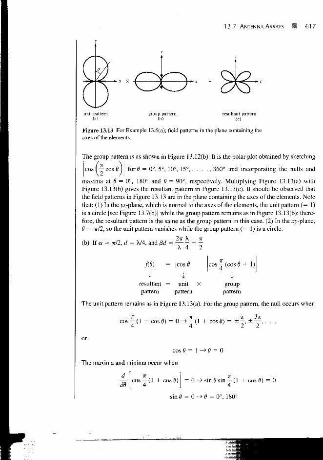
13.7 ANTENNA ARRAYS • 617

group pattern(b)

resultant pattern(c)

Figure 13.13 For Example 13.6(a); field patterns in the plane containing theaxes of the elements.

The group pattern is as shown in Figure 13.12(b). It is the polar plot obtained by sketching

for0 = 0°, 5°, 10°, 15°,. . . . , 360° and incorporating the nulls andcos ( — cos 0

maxima at 0 = 0°, 180° and 0 = 90°, respectively. Multiplying Figure 13.13(a) withFigure 13.13(b) gives the resultant pattern in Figure 13.13(c). It should be observed thatthe field patterns in Figure 13.13 are in the plane containing the axes of the elements. Notethat: (1) In the yz-plane, which is normal to the axes of the elements, the unit pattern (= 1)is a circle [see Figure 13.7(b)] while the group pattern remains as in Figure 13.13(b); there-fore, the resultant pattern is the same as the group pattern in this case. (2) In the xy-plane,0 = 7r/2, SO the unit pattern vanishes while the group pattern (= 1) is a circle.

(b) If a = TT/2, d = A/4, and fid = — - = -A 4 2

c o s — ( c o s 0 + 1 )

Igrouppattern

I iresultant = unit Xpattern pattern

The unit pattern remains as in Figure 13.13(a). For the group pattern, the null occurs when

COS j (1 + COS 6>) = 0 -> - (1 + COS 0) = ± y , ±-y, . . .

or

cos 8 = 1 -» 0 = 0

The maxima and minima occur when

— cos - (1 + cos 0) = 0 -» sin 0 sin - (1 + cos 0) = 0dd I 4 J 4

sin0 = O->0 = 0°, 180°

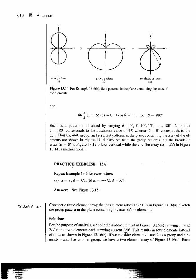
618 • Antennas

x X

unit pattern(a)

group pattern(b)

resultant pattern(c)

Figure 13.14 For Example 13.6(b); field patterns in the plane containing the axes ofthe elements.

and

sin — (1 + cos 6) = 0 —> cos I= - 1 or 6 = 180°

Each field pattern is obtained by varying 0 = 0°, 5°, 10°, 15°,. . ., 180°. Note that8 = 180° corresponds to the maximum value of AF, whereas d = 0° corresponds to thenull. Thus the unit, group, and resultant patterns in the plane containing the axes of the el-ements are shown in Figure 13.14. Observe from the group patterns that the broadsidearray (a = 0) in Figure 13.13 is bidirectional while the end-fire array (a = (3d) in Figure13.14 is unidirectional.

PRACTICE EXERCISE 13.6

Repeat Example 13.6 for cases when:

(a) a = IT, d = A/2, (b) a = -TT/2, d = A/4.

Answer: See Figure 13.15.

EXAMPLE 13.7 Consider a three-element array that has current ratios 1:2:1 as in Figure 13.16(a). Sketchthe group pattern in the plane containing the axes of the elements.

Solution:

For the purpose of analysis, we split the middle element in Figure 13.16(a) carrying current27/0° into two elements each carrying current 1/0^. This results in four elements insteadof three as shown in Figure 13.16(b). If we consider elements 1 and 2 as a group and ele-ments 3 and 4 as another group, we have a two-element array of Figure 13.16(c). Each

13.7 ANTENNA ARRAYS • 619

x X

x X

(a)

(b)

Figure 13.15 For Practice Exercise 13.6.

//0 2IlQ_ //O Figure 13.16 For Example 13.7: (a) a three-element array• ,_ * ^ ; i J with current ratios 1:2:1; (b) and (c) equivalent two-element

-X/2- • X / 2 -

(a)arrays.

3 *

2»

(b)

4

1,2 3 , 4* *

(c)

620 Antennas

group is a two-element array with d — X/2, a = 0, that the group pattern of the two-element array (or the unit pattern for the three-element array) is as shown in Figure13.13(b). The two groups form a two-element array similar to Example 13.6(a) withd = X/2, a = 0, so the group pattern is the same as that in Figure 13.13(b). Thus, in thiscase, both the unit and group patterns are the same pattern in Figure 13.13(b). The resultantgroup pattern is obtained in Figure 13.17(c). We should note that the pattern in Figure13.17(c) is not the resultant pattern but the group pattern of the three-element array. The re-sultant group pattern of the array is Figure 13.17(c) multiplied by the field pattern of theelement type.

An alternative method of obtaining the resultant group pattern of the three-elementarray of Figure 13.16 is following similar steps taken to obtain eq. (13.59). We obtain thenormalized array factor (or the group pattern) as

(AF)n = -

_\_~ 4_ J_~ 2

2el*

e'1*

c o s -

where yj/ = fid cos d + a if the elements are placed along the z-axis but oriented parallel to2TT X

the x-axis. Since a = 0, d = X/2, fid = — • — = x,X 2

(AF)n

{AF)n

Iresultant

group pattern

cos ( — cos 6

cos | — cos i

4unit

patternX

cos ( — cos 0

4grouppattern

The sketch of these patterns is exactly what is in Figure 13.17.If two three-element arrays in Figure 13.16(a) are displaced by X/2, we obtain a four-

element array with current ratios 1:3:3:1 as in Figure 13.18. Two of such four-element

Figure 13.17 For Example 13.7; obtain-ing the resultant group pattern of thethree-element array of Figure 13.16(a).

unit pattern

(a)

roup pattern

(b)

resultant grouppattern

(0

13.8 EFFECTIVE AREA AND THE FRIIS EQUATION 621

3//0_

-X/2-

/ [0_ Figure 13.18 A four-elementarray with current ratios 1:3:3:1;for Practice Exercise 13.7.

arrays, displaced by X/2, give a five-element array with current ratios 1:4:6:4:1. Contin-uing this process results in an /^-element array, spaced X/2 and (N - l)X/2 long, whosecurrent ratios are the binomial coefficients. Such an array is called a linear binomial army.

PRACTICE EXERCISE 13.7

(a) Sketch the resultant group pattern for the four-element array with current ratios1:3:3:1 shown in Figure 13.18.

(b) Derive an expression for the group pattern of a linear binomial array of N ele-ments. Assume that the elements are placed along the z-axis, oriented parallel to the;t-axis with spacing d and interelement phase shift a.

Answer: (a) See Figure 13.19, (b) c o s - , where if/ — fid cos d + a.

Figure 13.19 For Practice Exercise 13.7(a).

'13.8 EFFECTIVE AREA AND THE FRIIS EQUATION

In a situation where the incoming EM wave is normal to the entire surface of a receivingantenna, the power received is

Pr = (13.67)

But in most cases, the incoming EM wave is not normal to the entire surface of theantenna. This necessitates the idea of the effective area of a receiving antenna.

The concept of effective area or effective aperture (receiving cross section of anantenna) is usually employed in the analysis of receiving antennas.

The effective area A, of u receiving antenna is the ratio of the time-average powerreceived Pr (or delivered to (he load, to be strict) to the time-average power density;?„,, of the incident wave at the antenna.

622 Antennas

That is

PrOb•J avp

(13.68)

From eq. (13.68), we notice that the effective area is a measure of the ability of the antennato extract energy from a passing EM wave.

Let us derive the formula for calculating the effective area of the Hertzian dipoleacting as a receiving antenna. The Thevenin equivalent circuit for the receiving antenna isshown in Figure 13.20, where Voc is the open-circuit voltage induced on the antenna termi-nals, Zin = 7?rad + jXin is the antenna impedance, and ZL = RL + jXL is the external loadimpedance, which might be the input impedance to the transmission line feeding theantenna. For maximum power transfer, ZL = Z*n and XL = —Xin. The time-average powerdelivered to the matched load is therefore

'rad

|v«(13.69)

8 D"ra .

For the Hertzian dipole, Rmd = S0ir2(dl/X)2 and yoc = Edl where E is the effective fieldstrength parallel to the dipole axis. Hence, eq. (13.69) becomes

Pr =E\2

640TT2

The time-average power at the antenna is

_ave "

2TJ0 240TT

Inserting eqs. (13.70) and (13.71) in eq. (13.68) gives

3X2 X2

A L 5

(13.70)

(13.71)

or

(13.72)

Figure 13.20 Thevenin equivalent of a receivingantenna.

13.8 EFFECTIVE AREA AND THE FRIIS EQUATION 623

where D = 1.5 is the directivity of the Hertzian dipole. Although eq. (13.72) was derivedfor the Hertzian dipole, it holds for any antenna if D is replaced by GJfi, (j>). Thus, ingeneral

(13.73)

Now suppose we have two antennas separated by distance r in free space as shown inFigure 13.21. The transmitting antenna has effective area Aet and directive gain Gdt, andtransmits a total power P, (= Prli<i). The receiving antenna has effective area of Aer and di-rective gain Gdn and receives a total power of Pr. At the transmitter,

4rU

P

or

op =ave

p(13.74)

By applying eqs. (13.68) and (13.73), we obtain the time-average power received as

P = Op A = ^— C,,r r ^ ave ^er * ^dr

Substituting eq. (13.74) into eq. (13.75) results in

(13.75)

(13.76)

This is referred to as the Friis transmission formula. It relates the power received by oneantenna to the power transmitted by the other, provided that the two antennas are separatedby r > 2d2l\, where d is the largest dimension of either antenna [see eq. 13.52)]. There-fore, in order to apply the Friis equation, we must make sure that the two antennas are inthe far field of each other.

Transmitter Receiver

H r-

Figure 13.21 Transmitting and receiving antennas in free space.

624 Antennas

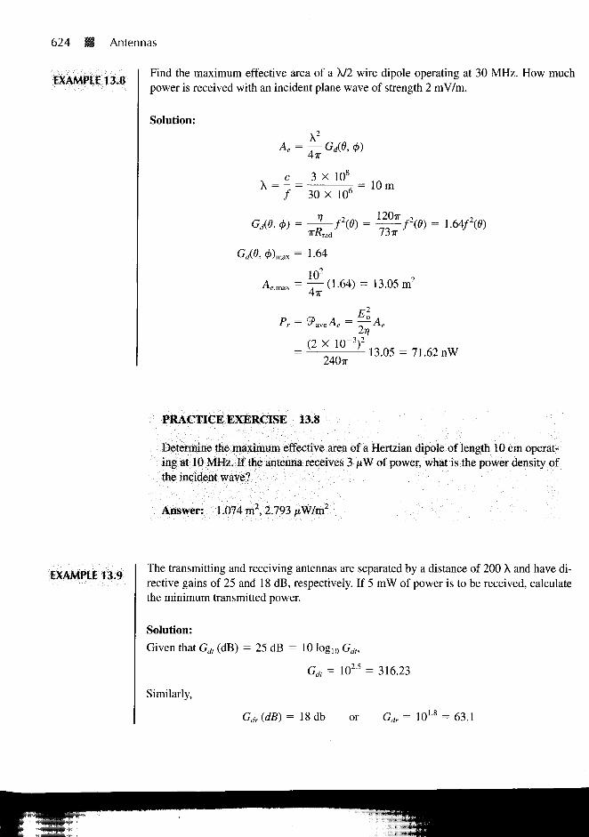
EXAMPLE 13.8Find the maximum effective area of a A/2 wire dipole operating at 30 MHz. How muchpower is received with an incident plane wave of strength 2 mV/m.

Solution:

c 3 X 108

A = - = T = 10m/ 30 X 106

Gd(6, 0)raax = 1.64

102

(1.64)= 13.05 m2

p = Op A - — A

_ V

( 2 X 1 0 )

= 1.64/(0)

240TT13.05 = 71.62 nW

PRACTICE EXERCISE 13.8

Determine the maximum effective area of a Hertzian dipole of length 10 cm operat-ing at 10 MHz. If the antenna receives 3 [iW of power, what is the power density ofthe incident wave?

Answer: 1.074 m2, 2.793 MW/m2

EXAMPLE 13.9The transmitting and receiving antennas are separated by a distance of 200 A and have di-rective gains of 25 and 18 dB, respectively. If 5 mW of power is to be received, calculatethe minimum transmitted power.

Solution:

Given that Gdt (dB) = 25 dB = 10 log10 Gdt,

Gdt = 1025 = 316.23

Similarly,

Gdr (dB) = 18 db or Gdr = 1 0 ° = 63.1

13.9 THE RADAR EQUATION 625

Using the Friis equation, we have

or

P = P

Pr ~ GdrGdt [ — J P,

47rr12

= 5 x 10~3

= 1.583 W

J GdrGdt4TT X 200 X

X

1(63.1X316.23)

PRACTICE EXERCISE 13.9

An antenna in air radiates a total power of 100 kW so that a maximum radiated elec-tric field strength of 12 mV/m is measured 20 km from the antenna. Find: (a) its di-rectivity in dB, (b) its maximum power gain if r]r =

Answer: (a) 3.34 dB, (b) 2.117.

13.9 THE RADAR EQUATION

Radars are electromagnetic devices used for detection and location of objects. The termradar is derived from the phrase radio detection and ranging. In a typical radar systemshown in Figure 13.22(a), pulses of EM energy are transmitted to a distant object. Thesame antenna is used for transmitting and receiving, so the time interval between the trans-mitted and reflected pulses is used to determine the distance of the target. If r is the dis-

k Target a

Figure 13.22 (a) Typical radar system,(b) simplification of the system in(a) for calculating the target crosssection a.

(b)

626 Antennas

tance between the radar and target and c is the speed of light, the elapsed time between thetransmitted and received pulse is 2r/c. By measuring the elapsed time, r is determined.

The ability of the target to scatter (or reflect) energy is characterized by the scatteringcross section a (also called the radar cross section) of the target. The scattering crosssection has the units of area and can be measured experimentally.

The scattering cross section is the equivalent area intercepting that amount olpower that, when scattering isotropicall). produces at the radar a power density,which is equal to thai scattered (or reflected) by the actual target.

That is,

= lim4-irr2

or

<3/>a = lim 4xr2 —-

9>(13.77)

where SP, is the incident power density at the target T while 3 \ is the scattered powerdensity at the transreceiver O as in Figure 13.22(b).

From eq. (13.43), the incident power density 2P, at the target Tis

op = op = d p J^ i "^ ave , 9 * rad

4TIT

The power received at transreceiver O is

(13.78)

or

—Aer

(13.79)

Note that 2P, and 9 \ are the time-average power densities in watts/m2 and Prad and Pr arethe total time-average powers in watts. Since Gdr = Gdt — Gd and Aer = Aet = Ae, substi-tuting eqs. (13.78) and (13.79) into eq. (13.77) gives

a = (4irr2)2 1Gd

or

AeaGdPmd

(4irr2)2

(13.80a)

(13.80b)

13.9 THE RADAR EQUATION 627

TABLE 13.1 Designationsof Radar Frequencies

Designation

UHF

L

S

C

X

Ku

K

Millimeter

Frequency

300-1000 MHz

1000-2000 MHz

2000^000 MHz

4000-8000 MHz

8000-12,500 MHz

12.5-18 GHz

18-26.5 GHz>35 GHz

From eq. (13.73), Ae = \2GJAi;. Hence,

(13.81)

This is the radar transmission equation for free space. It is the basis for measurement ofscattering cross section of a target. Solving for r in eq. (13.81) results in

(13.82)

Equation (13.82) is called the radar range equation. Given the minimum detectable powerof the receiver, the equation determines the maximum range for a radar. It is also useful forobtaining engineering information concerning the effects of the various parameters on theperformance of a radar system.

The radar considered so far is the monostatic type because of the predominance of thistype of radar in practical applications. A bistatic radar is one in which the transmitter andreceiver are separated. If the transmitting and receiving antennas are at distances rx and r2

from the target and Gdr ¥= Gdt, eq. (13.81) for bistatic radar becomes

GdtGdr

4TTrad (13.83)

Radar transmission frequencies range from 25 to 70,000 MHz. Table 13.1 shows radarfrequencies and their designations as commonly used by radar engineers.

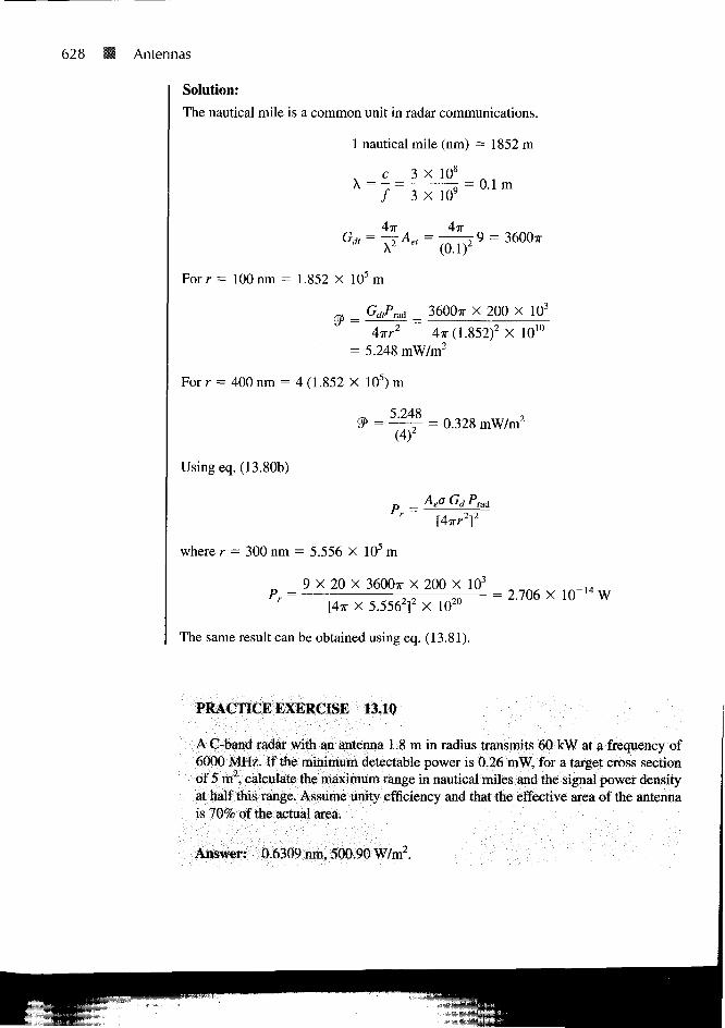
EXAMPLE 13.10An S-band radar transmitting at 3 GHz radiates 200 kW. Determine the signal powerdensity at ranges 100 and 400 nautical miles if the effective area of the radar antenna is9 m2. With a 20-m2 target at 300 nautical miles, calculate the power of the reflected signalat the radar.

628 Antennas

Solution:

The nautical mile is a common unit in radar communications.

1 nautical mile (nm) = 1852 m

c 3 X 108

/ 3 X 10-

r -X2 et (0.1):

= 0.1m

9 = 3600?r

For r = 100 nm = 1.852 X 105m

ad 3600TT X 200 X 103

4TIT2 4TT(1 .852) 2 X 1010

= 5.248 mW/m2

For r = 400 nm = 4 (1.852 X 105) m

5.248

(4)2 = 0.328 mW/m2

Aea Gd P r a d

Using eq. (13.80b)

where r = 300 nm = 5.556 X 105 m

_ 9 X 20 X 36007T X 200 X 103

[4TT X 5.5562]2 X 1020

The same result can be obtained using eq. (13.81).

= 2.706 X 10"14W

PRACTICE EXERCISE 13.10

A C-band radar with an antenna 1.8 m in radius transmits 60 kW at a frequency of6000 MHz. If the minimum detectable power is 0.26 mW, for a target cross sectionof 5 m2, calculate the maximum range in nautical miles and the signal power densityat half this range. Assume unity efficiency and that the effective area of the antennais 70% of the actual area.

Answer: 0.6309 nm, 500.90 W/m2.

SUMMARY 629

SUMMARY 1. We have discussed the fundamental ideas and definitions in antenna theory. The basictypes of antenna considered include the Hertzian (or differential length) dipole, thehalf-wave dipole, the quarter-wave monopole, and the small loop.

2. Theoretically, if we know the current distribution on an antenna, we can find the re-tarded magnetic vector potential A, and from it we can find the retarded electromag-netic fields H and E using

H = V X — , E = T, H X a*

The far-zone fields are obtained by retaining only \lr terms.3. The analysis of the Hertzian dipole serves as a stepping stone for other antennas. The

radiation resistance of the dipole is very small. This limits the practical usefulness ofthe Hertzian dipole.

4. The half-wave dipole has a length equal to X/2. It is more popular and of more practi-cal use than the Hertzian dipole. Its input impedance is 73 + J42.5 fi.

5. The quarter-wave monopole is essentially half a half-wave dipole placed on a con-ducting plane.

6. The radiation patterns commonly used are the field intensity, power intensity, and ra-diation intensity patterns. The field pattern is usually a plot of \ES\ or its normalizedform flft). The power pattern is the plot of 2Pave or its normalized form/2(0).

7. The directive gain is the ratio of U(9, <f>) to its average value. The directivity is themaximum value of the directive gain.

8. An antenna array is a group of radiating elements arranged so as to produce someparticular radiation characteristics. Its radiation pattern is obtained by multiply-ing the unit pattern (due to a single element in the group) with the group pattern,which is the plot of the normalized array factor. For an TV-element linear uniformarray,

AF =

where \j/ = 13d cos 9 + a, 0 = 2%/X, d = spacing between the elements, and a = in-terelement phase shift.

9. The Friis transmission formula characterizes the coupling between two antennas interms of their directive gains, separation distance, and frequency of operation.

10. For a bistatic radar (one in which the transmitting and receiving antennas are sepa-rated), the power received is given by

4TTrJ

aPn•ad

For a monostatic radar, r, = r2 = r and Gdt = Gdr.

630 Antennas

13.1 An antenna located in a city is a source of radio waves. How much time does it take thewave to reach a town 12,000 km away from the city?

(a) 36 s

(b) 20 us

(c) 20 ms

(d) 40 ms

(e) None of the above

13.2 In eq. (13.34), which term is the radiation term?

(a) 1/rterm

(b) l/r2term

(c) IIr" term

(d) All of the above

13.3 A very small thin wire of length X/100 has a radiation resistance of

(a) = 0 G

(b) 0.08 G

(c) 7.9 G

(d) 790 0

13.4 A quarter-wave monopole antenna operating in air at frequency 1 MHz must have anoverall length of

(a) € » X

(b) 300 m

(c) 150 m

(d) 75 m

(e) ( <sC X

13.5 If a small single-turn loop antenna has a radiation resistance of 0.04 G, how many turnsare needed to produce a radiation resistance of 1 G?

(a) 150

(b) 125

(c) 50

(d) 25

(e) 5

REVIEW QUESTIONS 631

13.6 At a distance of 8 km from a differential antenna, the field strength is 12 /iV/m. The fieldstrength at a location 20 km from the antenna is

(a) 75/xV/m

(b) 30,xV/m

(c) 4.8/xV/m

(d) 1.92/zV/m

13.7 An antenna has f/max = 10 W/sr, l/ave = 4.5 W/sr, and i\r = 95%. The input power tothe antenna is

(a) 2.222 W

(b) 12.11 W

(c) 55.55 W

(d) 59.52 W

13.8 A receiving antenna in an airport has a maximum dimension of 3 m and operates at 100MHz. An aircraft approaching the airport is 1/2 km from the antenna. The aircraft is inthe far field region of the antenna.

(a) True

(b) False

13.9 A receiving antenna is located 100 m away from the transmitting antenna. If the effectivearea of the receiving antenna is 500 cm2 and the power density at the receiving locationis 2 mW/m2, the total power received is:

(a) lOnW

(b) 100 nW

(c) 1/xW

(d) 10 ^W

(e) 100 ^W

13.10 Let R be the maximum range of a monostatic radar. If a target with radar cross section of5 m2 exists at R/2, what should be the target cross section at 3R/2 to result in an equalsignal strength at the radar?

(a) 0.0617 m2

(b) 0.555 m2

(c) 15 m2

(d) 45 m2

(e) 405 m2

Answers: 13.Id, 13.2a, 13.3b, 13.4d, 13.5e, 13.6c, 13.7d, 13.8a, 13.9e, 13.10e.

632 • Antennas

PROBLEMS I13.1 The magnetic vector potential at point P(r, 8, <j>) due to a small antenna located at the

origin is given by

50 e->Br

A

where r2 = x2 + y2 + z2• Find E(r, 6, <j>, t) and H(r, d, <j>, i) at the far field.

13.2 A Hertzian dipole at the origin in free space has di = 20 c m and 7 = 1 0 cos 2irl07t A ,find \E6s\ at the distant point (100 , 0, 0 ) .

13.3 A 2-A source operating at 300 MHz feeds a Hertzian dipole of length 5 mm situated atthe origin. Find Es and H,. at (10, 30°, 90°).

13.4 (a) Instead of a constant current distribution assumed for the short dipole of Section

13.2, assume a triangular current distribution 7, = 7O I 1 — j shown in Figure

13.23. Show that

?rad = 2 0 7TZ I -

which is one-fourth of that in eq. (13.13). Thus Rmd depends on the current distribu-tion.

(b) Calculate the length of the dipole that will result in a radiation resistance of 0.5 0.

13.5 An antenna can be modeled as an electric dipole of length 5 m at 3 MHz. Find the radia-tion resistance of the antenna assuming a uniform current over its length.

13.6 A half-wave dipole fed by a 50-0 transmission line, calculate the reflection coefficientand the standing wave ratio.

13.7 A 1-m-long car radio antenna operates in the AM frequency of 1.5 MHz. How muchcurrent is required to transmit 4 W of power?

Figure 13.23 Short dipole antenna with triangular current distri-bution; for Problem 13.4.

PROBLEMS • 633

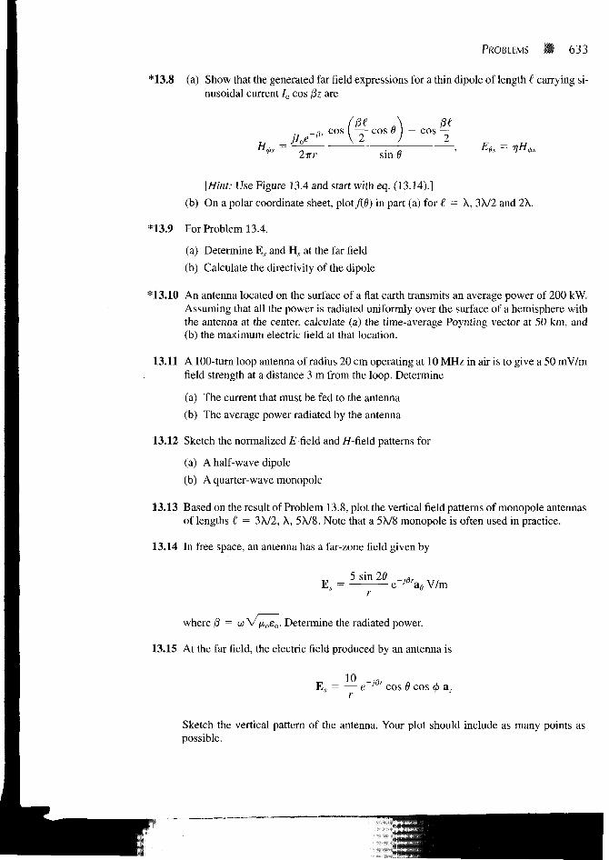
*13.8 (a) Show that the generated far field expressions for a thin dipole of length € carrying si-nusoidal current Io cos @z are

,-/3rCos^ Yc0St)J ~ c o s y2-wr sin 8

[Hint: Use Figure 13.4 and start with eq. (13.14).]

(b) On a polar coordinate sheet, plot fifi) in part (a) for € = X, 3X/2 and 2X.

*13.9 For Problem 13.4.

(a) Determine E, and H s at the far field

(b) Calculate the directivity of the dipole

*13.10 An antenna located on the surface of a flat earth transmits an average power of 200 kW.Assuming that all the power is radiated uniformly over the surface of a hemisphere withthe antenna at the center, calculate (a) the time-average Poynting vector at 50 km, and(b) the maximum electric field at that location.

13.11 A 100-turn loop antenna of radius 20 cm operating at 10 MHz in air is to give a 50 mV/mfield strength at a distance 3 m from the loop. Determine

(a) The current that must be fed to the antenna

(b) The average power radiated by the antenna

13.12 Sketch the normalized E-field and //-field patterns for

(a) A half-wave dipole

(b) A quarter-wave monopole

13.13 Based on the result of Problem 13.8, plot the vertical field patterns of monopole antennasof lengths € = 3X/2, X, 5X/8. Note that a 5X/8 monopole is often used in practice.

13.14 In free space, an antenna has a far-zone field given by

where /3 = wV/xoeo. Determine the radiated power.

13.15 At the far field, the electric field produced by an antenna is

E s = — e~j/3r cos 6 cos <j> az

Sketch the vertical pattern of the antenna. Your plot should include as many points aspossible.

634 Antennas

13.16 For an Hertzian dipole, show that the time-average power density is related to the radia-tion power according to

1.5 sin20 _

4irr

13.17 At the far field, an antenna produces

2 sin 6 cos 4>ave a r W/m2, 0 < 6 < x, 0 < </> < x/2

Calculate the directive gain and the directivity of the antenna.

13.18 From Problem 13.8, show that the normalized field pattern of a full-wave (€ = X)antenna is given by

cos(x cos 6) + 1sin0

Sketch the field pattern.

13.19 For a thin dipole A/16 long, find: (a) the directive gain, (b) the directivity, (c) the effec-tive area, (d) the radiation resistance.

13.20 Repeat Problem 13.19 for a circular thin loop antenna A/12 in diameter.

13.21 A half-wave dipole is made of copper and is of diameter 2.6 mm. Determine the effi-ciency of the dipole if it operates at 15 MHz.Hint: Obtain R( from R(/Rdc = a/28; see Section 10.6.

13.22 Find C/ave, t/max, and D if:

(a) Uifi, 4>) = sin2 20, 0 < 0 < x, 0 < 0 < 2TT

(b) Uifi, <t>) = 4 esc2 20, TT/3 < 0 < x/2, 0 < <j> < x

(c) U(6, 4>) = 2 sin2 0 sin2 <j>, 0 < d < x, 0 < <t> < x

13.23 For the following radiation intensities, find the directive gain and directivity:

(a) U(6, 4>) = s in 2 0, 0 < 0 < x, 0 < <j> < 2x

(b) U(6, <t>) = 4 sin2 0 c o s 2 0 , O < 0 < T T , 0 < 0 < TT

(c) Uifi, <t>) = 10 cos2 0 sin2 4>/2, 0 < 0 < x, 0 < <f> < x/2

13.24 In free space, an antenna radiates a field

4TIT

at far field. Determine: (a) the total radiated power, (b) the directive gain at 0 = 60°.

13.25 Derive Es at far field due to the two-element array shown in Figure 13.24. Assume thatthe Hertzian dipole elements are fed in phase with uniform current /o cos cot.

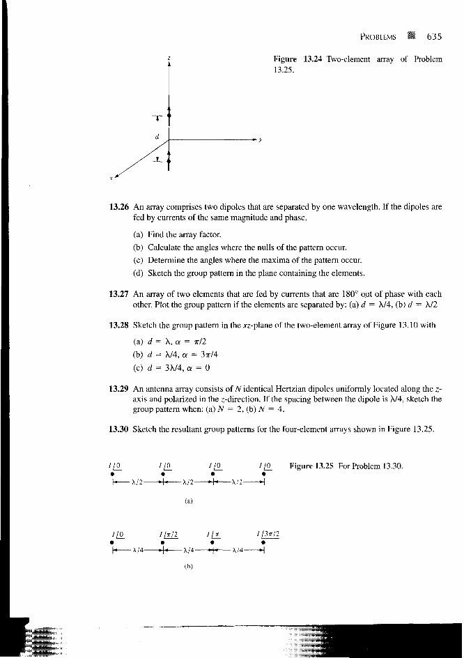
PROBLEMS 635

Figure 13.24 Two-element array of Problem13.25.

-*-y

13.26 An array comprises two dipoles that are separated by one wavelength. If the dipoles arefed by currents of the same magnitude and phase,

(a) Find the array factor.

(b) Calculate the angles where the nulls of the pattern occur.

(c) Determine the angles where the maxima of the pattern occur.

(d) Sketch the group pattern in the plane containing the elements.

13.27 An array of two elements that are fed by currents that are 180° out of phase with eachother. Plot the group pattern if the elements are separated by: (a) d = A/4, (b) d = X/2

13.28 Sketch the group pattern in the xz-plane of the two-element array of Figure 13.10 with

(a) d = A, a = -all

(b) d = A/4, a = 3TT/4

(c) d = 3A/4, a = 0

13.29 An antenna array consists of N identical Hertzian dipoles uniformly located along the z-axis and polarized in the ^-direction. If the spacing between the dipole is A/4, sketch thegroup pattern when: (a) N = 2, (b) N = 4.

13.30 Sketch the resultant group patterns for the four-element arrays shown in Figure 13.25.

- X / 2 - -X/2-

(a)

'12. l[0_ Figure 13.25 For Problem 13.30.

x/2-

'12.•X/4-

I jit 12

-X/4-

(b)

//3ir/2

-X/4-

636 • Antennas

13.31 For a 10-turn loop antenna of radius 15 cm operating at 100 MHz, calculate the effectivearea at $ = 30°, <j> = 90°.

13.32 An antenna receives a power of 2 /xW from a radio station. Calculate its effective area ifthe antenna is located in the far zone of the station where E = 50 mV/m.

13.33 (a) Show that the Friis transmission equation can be written as

"r _ AerAet

(b) Two half-wave dipole antennas are operated at 100 MHz and separated by 1 km. If80 W is transmitted by one, how much power is received by the other?

13.34 The electric field strength impressed on a half-wave dipole is 3 mV/m at 60 MHz. Cal-culate the maximum power received by the antenna. Take the directivity of the half-wavedipole as 1.64.

13.35 The power transmitted by a synchronous orbit satellite antenna is 320 W. If the antennahas a gain of 40 dB at 15 GHz, calculate the power received by another antenna with again of 32 dB at the range of 24,567 km.

13.36 The directive gain of an antenna is 34 dB. If the antenna radiates 7.5 kW at a distance of40 km, find the time-average power density at that distance.

13.37 Two identical antennas in an anechoic chamber are separated by 12 m and are orientedfor maximum directive gain. At a frequency of 5 GHz, the power received by one is 30dB down from that transmitted by the other. Calculate the gain of the antennas in dB.

13.38 What is the maximum power that can be received over a distance of 1.5 km in free spacewith a 1.5-GHz circuit consisting of a transmitting antenna with a gain of 25 dB and a re-ceiving antenna with a gain of 30 dB? The transmitted power is 200 W.

13.39 An L-band pulse radar with a common transmitting and receiving antenna having a di-rective gain of 3500 operates at 1500 MHz and transmits 200 kW. If the object is 120 kmfrom the radar and its scattering cross section is 8 m2, find

(a) The magnitude of the incident electric field intensity of the object

(b) The magnitude of the scattered electric field intensity at the radar

(c) The amount of power captured by the object

(d) The power absorbed by the antenna from the scattered wave

13.40 A transmitting antenna with a 600 MHz carrier frequency produces 80 W of power. Findthe power received by another antenna at a free space distance of 1 km. Assume both an-tennas has unity power gain.

13.41 A monostable radar operating at 6 GHz tracks a 0.8 m2 target at a range of 250 m. If thegain is 40 dB, calculate the minimum transmitted power that will give a return power of2/tW.

PROBLEMS 637

13.42 In the bistatic radar system of Figure 13.26, the ground-based antennas are separated by4 km and the 2.4 m2 target is at a height of 3 km. The system operates at 5 GHz. For Gdt

of 36 dB and Gdr of 20 dB, determine the minimum necessary radiated power to obtain areturn power of 8 X 10~12W.

Scatteredwave

Receivingantenna

Target a Figure 13.26 For Problem 13.42.

3 km

Transmittingantenna