Chapter 12. Using regression models in epidemiologic analysis

Chapter 12. Using regression models in epidemiologic analysis

January 20, 2022Epidemiology (14)

Minato Nakazawa<[email protected]>

To make the graphs in this slide, you can usehttps://minato.sip21c.org/epispecial/codes-for-Chapter12.R

Application of simple mathematical model

● Figure 12-1 is an example of simple linear regression.

● The 2 primary purposes of models in epidemiology → Different models should be applied (though many courses in statistics may not distinguish those).

– To make prediction● Estimating the risk (or other epidemiologic measures) based on

information from risk predictors.

– To control for confounding● Aiming at learning about the causal role of few specific factors for

disease, simultaneously controlling for possible confounding effects of other factors.

● Figure 12-1 shows almost perfect linear regression. Regression line means that estimated average values for the variable on the vertical scale (Y) according to values of the variable on the horizontal scale (X) in the form of:

Y-hat is the estimated value of Y for any given values of X. The a0 is

the intercept and a1 is the coefficient of X, which means the slope (=

the number of units of change in Y-hat for every unit change in X). The intercept 1.15 (/100000) means the age-standardized mortality rates in the absence of cigarette smoking. According to the raw data, it was 0.6 (/100000) in the absence of smoking, slightly different from the estimated 1.15, which uses all five data points.The slope 0.282 means the increment of deaths per 100000 for every additional cigarette smoking daily.

Assuming that confounding and other biases were properly addressed, the slope quantifies the effect of cigarette smoking on laryngeal cancer. The line also gives estimate of mortality rate ratios. Age-standardized mortality rate of 15.2 (/100000, which is 1.15 + 0.282 x 50) for 50 cigarettes daily is 15.2/1.15 = 13.3 times larger than the rate in nonsmokers.

THE GENERAL LINEAR MODEL● Models with more than 1 factor at a time can be used as an alternative to

stratification to control confounding.

● As extension of linear model of Figure 12-1,

● Y is dependent variable. X1 and X

2 are independent variables.

● Suppose that Y is the age standardized mortality rate of laryngeal cancer in Figure 12-1, and that X

1 is the number of cigarettes smoked per day, then X

2 may be the

amount of alcohol consumed per day (Alcohol drinking is also risk of laryngeal cancer): The multiple regression line can be drawn in 3D space.

● Since cigarette smoking and alcohol drinking are correlated and thus those are mutually confounding risk factors for laryngeal cancer.

● A stratified analysis can remove that confounding, but the confounding can also be removed by fitting [12-1]. The coefficients for X1 and X2 (a1 and a

2) are

unconfounded.

● The general form of [12-1] is “general linear model”.

TRANSFORMING THE GENERAL LINEAR MODEL

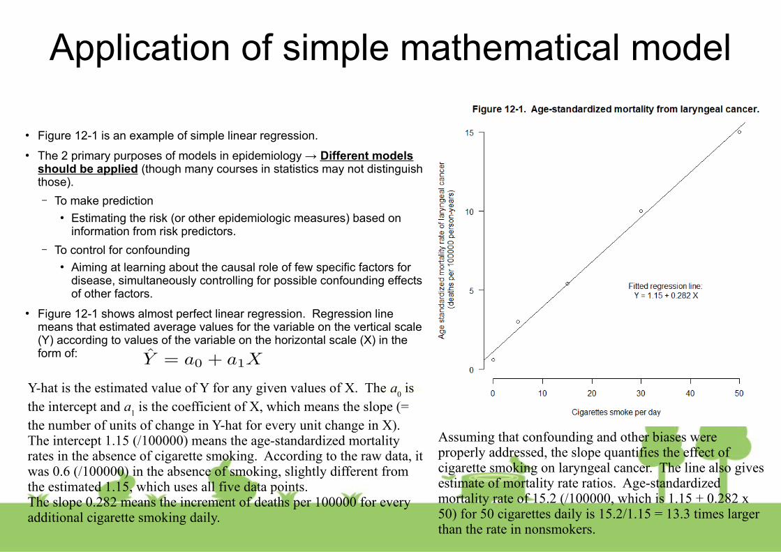
● Dependent variable in a regression model is not mathematically constrained.

● However, in actual study, the range of variable is constrained by many ways

– FEV1 (Forced expiratory volume in 1 sec, a measure of lung function) cannot take negative value.

– Disease occurrence (no/yes) is usually assigned a value of 0/1. To avoid getting impossible values (eg., negative mortality rate) for the dependent variable, fit straight line to the logarithm of the mortality rate is possible, as [12-2], where ln(Y-hat) is natural logarithm of Y-hat. By taking antilogarithm of [12-2], [12-3] is obtained. This is exponential model.

– In linear model, effect of exposure is simply obtained as the difference of Y-hats for X=0 and X=1, it’s the slope of the regression line.

– In exponential model, the ratio of Y-hat (rate ratio of exposed to unexposed persons) is antilogarithm of the coefficient.

THE LOGISTIC TRANSFORMATION

● If risk data is obtained, the range is much narrower. Rates are never negative but can go as high as infinity, but risks range [0, 1].

● Converting [0, 1] to (-∞, ∞) is possible by logistic transformation.

● Risk odds, R/(1-R), range [0, ∞). Then take logarithm, it ranges (-∞, ∞).

● ln[R/(1-R)] is a “logit” of R. This 2 step transformation is logistic transformation.

● The logistic model is that the logit is dependent variable of a straight line equation as [12-4]. If independent variable is more than one, it becomes “multiple logistic model”. The ratio is equal to the logarithm of the risk-odds ratio as [12-5]. The result means that, in the logistic model, antilogarithm of the coefficient of a dichotomous exposure term estimates the odds ratio of risks.

CHOICES AMONG MODELS● From a practical standpoint, the transformations dictate what type

of measure the coefficients in the model will estimate.

– For risk data, the logistic model will provide odds ratio, not easily get the estimate of risk difference.

– The model is used to assess the risk for people, invalid (negative or more than 100%) estimates has to be avoided.

– The model is used to assess the overall effect of exposure and the ratio can be taken as effect measure, logistic model is appropriate.

● Consider the data in Table 12-1 (hypothetical risk data over 5 year period for 20 subjects with different ages ranging from 18 yrs to 77 yrs).

– If linear model is applied (Figure 12-2), the value of the intercept -0.49 is impossible value for a risk (all ages less than 24 or greater than 74 yrs give impossible estimates of risk).

– If logistic model is applied (Figure 12-3), direct estimation of a risk difference is impossible, but an odds-ratio associated with a 1-year increase in age is exp(0.144)=1.16 (by R, it’s 1.15500…)

● The logistic model is particularly appropriate for the analysis of case-control studies. Odds ratio can be obtained from case-control studies and used as an estimate of rate ratios if control is sampled adequately.

CONTROL OF CONFOUNDING WITH REGRESSION MODELS

● Multiple regression models can control several confounding variables simultaneously.

● As explained in Chapter 10, stratified analysis tends to require large sample size. Five confounding variables, each of which had 3 categories, generates 3x3x3x3x3=243 strata. To keep enough sample size within each stratum, total size becomes very large.

● Multiple regression modeling solves this problem, though the results from the regression model are readily susceptible to bias if the model is not a good fit to the data.

● Figure 12-4 and 12-5 show hypothetical data, with data for exposed and unexposed people by age and by some unspecified continuous outcome measure. Unfortunately, there is no overlap in the age distributions between exposed and unexposed.

– Stratified analysis would produce no estimate of effect (No information in the data)

– Multiple linear regression with both age and exposure terms, which fit two parallel straight lines through the data, can show the difference in the outcome between exposed and unexposed as the coefficient for the exposure term (Figure 12-4). Regression model produces a statistically stable estimate from the nonoverlapping sets of data.

– However, the relation between age and outcome may be curvilinear (Figure 12-5). If so, the effect measure from multiple linear regression is incorrect. And, we cannot know whether the model in Figure 12-4 is appropriate or the model in Figure 12-5 is appropriate.

● If we have such nonoverlapping data, saying nothing is better than saying something incorrect. The result of stratified analysis is more reliable. By stratified analysis, the researcher and reader can see the distribution of the data by the key variable. Thus, the multiple regression analysis should be used only as a supplement to a stratified analysis.

● Multivariate model looks sophisticated and thus it’s a lure, but often leads to mistake.

PREDICTING RISK FOR A PERSON● Regression model is used to predict individual’s outcome.

● Murabito et al. (1997) [https://www.ncbi.nlm.nih.gov/pubmed/9236415]

– Logistic model for 4-year risk estimates for intermittent claudication (the symptomatic expression of atherosclerosis in the lower extremities), shown in Table 12-2.

– Getting individual risk estimates from this model, coefficient for each variable in the table is multiplied by the values for a given person and summed up, which gives logit for a given person. Then take exponential, risk-odds (R/(1-R)) is obtained.

– Odds = Risk/(1-Risk) ↔ Risk = Odd/(1+Odds)

– Then Risk is exp(logit)/[1+exp(logit)]

– The 4-year risk of intermittent claudication for a 70-year-old nonsmoking man with normal blood pressure, diabetes, coronary heart disease and cholesterol level of 250 mg/dL is obtained as

– logit = -8.915 + 1x0.503 + 70x0.037 + 0x0.000 + 1x0.950 + 0x0.031 + 250x0.005 + 1x0.994 = -2.628

– Risk = exp(-2.628)/[1+exp(-2.628)] = 0.067

– If the man had stage 2 hypertension, logit is -1.830 and Risk is 0.138.

● The purpose of including each individual term in the model in Table 12-2 is to improve the estimate of risk.

● Age nor presence of CHD is not a causal factor in this model, both are good predictors of the risk, it makes sense to include them in the prediction model.

Table 12-2. Logistic model to obtain estimates of 4-year risk for intermittent claudication

Variable Coefficient

Intercept - 8.915

Male sex 0.503

Age 0.037

Blood pressure

Normal 0.000

High-normal 0.262

Stage 1 hypertension 0.407

Stage 2 hypertension 0.798

Diabetes 0.950

Cigarettes / day 0.031

Cholesterol (mg/dL) 0.005

Coronary heart disease 0.994

STRATEGY FOR CONSTRUCTING REGRESSION MODELS FOR EPIDEMIOLOGIC ANALYSIS

● Centering of variables in regression models (box, p.223)

– The intercept in a regression model is the predicted outcome when all independent variables are 0.

– If 0 is not meaningful predictor, centering (convert the predicting variable around some central value) should be done.

● (eg.) Regression to predict mortality rates from BMI, BMI=0 makes no sense. Let the independent variable as (BMI – 22) instead of BMI itself, intercept is much more interpretable.

● Determine which confounders to include in the model

– First, all potential confounders are included

– Then, build a model by introducing predictor variables one at a time. After each term is introduced, examine the amount of change in the coefficient of the exposure term.

– If the exposure coefficient changes considerably (usually 10%), then the added variable is a confounder.

– It’s essential for the exposure to be included in the model as a single term (included as several terms or product terms should be avoided).

● Do a stratified analysis first

– The first step of the analysis should be a stratified analysis.

– Multivariable regression analysis contributes to causal research by enabling the simultaneous control of several confounding factors.

– Usually the confounding stems from one or two variables and a multivariable regression model will give essentially the same result as a properly conducted stratified analysis

● Stepwise models in epidemiologic analysis (box, p.234)

– Automatic selection based on statistical significance of each coefficient

– It may be valuable as prediction model

– For causal inference, using statistical significance for model selection must be avoided.

● Amount of confounding depends on the relation between the potential confounder and the exposure and the relation between the potential confounder and the outcome. Evaluation of coefficients only targets the latter.

● It may also omit confounding variables for which the relation with outcome is not statistically significant.

STRATEGY (cont’d) – Estimate the shape of the exposure-disease relation

● If the exposure variable is dichotomous, the effect of exposure is simply estimated as the coefficient, but if the exposure is continuous, redefinition of exposure is needed.

– If the model involves a logarithmic transformation, a single term for a continuous exposure variable mathematically takes the shape dictated by the model.

– In a logistic model, the exposure coefficient is the log of odds ratio for a unit change of exposure. The effect of the unit increase multiplies the odds ratio by a constant amount. The result is an exponential dose-response (Figure 12-6).

– Regardless of the actual shape of the relation between exposure and disease, the exponential shape fits the data if the exposure variable is continuous and included as single term in a model using a logarithmic transformation.

– In linear models, a linear relation is guaranteed.

● The shape of dose-response relation can be determined by data in several ways.

● Spline regression

– Using curve-smoothing like spline, a different fitted curve to apply in different ranges of the exposure.

● Avoiding to let the model determine the shape of relationship between exposure and disease is important.

● Factoring the exposure

– Categorizing exposure into ranges and then creating a separate term for each subrange of exposure, except for reference category.

– (eg.) Cigarette smoking can be categorized as zero/d, 1-9/d, 10-19/d, … According to the extent of smoking, each smoker can be categorized one of those categories (each category except 0 is treated as a dummy variable). Resulting set of coefficients in the fitted model indicate a separately estimated effect for each level.

● Evaluate interaction

– To evaluate interaction, redefinition of the two exposures by considering them jointly as a single composite exposure is needed.

– For two dichotomous exposure variables A and B, each person falls into one of the four categories, exposed to neither (as reference), exposed to A but not B, exposed to B but not A, exposed to both.

– By doing so, partitioning the risk or risk ratio among those with joint exposure to two agents into the four categories as explained in Chapter 11.

OVERFITTING OF REGRESSION MODELS AND SUMMARY CONFOUNDER SCORES

● Advantage of regression model is the ability to control simultaneously for several confounders

● One way to avoid overfitting is to use the summary confounder score.

– Disease risk score

– Exposure summary score (= propensity score)

● Rule of thumb: At least 10-15 observations for every term

● If less than that, overfitting may occur. The model is too heavily influenced by random error in the data.

● Trimming of the subjects outside the range of propensity scores that is common to both exposed and unexposed subjects (Figure 12-7)

Example of using propensity scores: Are drug-eluting stents better than bare-metal stents?

● Mauri et al. (2008) NEJM, 359: 1330-42.(https://www.nejm.org/doi/full/10.1056/NEJMoa0801485)

● Commented by many researchers including Rothman(https://www.nejm.org/doi/full/10.1056/NEJMc082174)

● Using the summary confounder score is popular in pharmacoepidemiology. Mauri et al. (2008) studied the comparative safety of two different kinds of stents (tubular wire cages used to keep arteries patent after narrowed vessels have been widened by angioplasty).

– Acute myocardial infarction adult patients at one hospital during 18 months

– Followed up 2 years after stenting

– Comparison between bare-metal stents and drug-eluting stents (to prevent scar tissue formation within the artery walls)

– Some differences in the characteristics of patients receiving the two kinds of stents.

– Each patient with drug-eluting stent was matched with a patient with bare-metal stent by propensity score. Though there should be no difference in risk of death within 2 days after stenting between 2 stents, 2-day risk for receiving bare-metal stent (1.2%) was almost double of that for drug-eluting stent (0.7%).

– Unfortunately, the authors incorrectly focused on the lack of statistical significance of the difference in 2-day risk of death. The P value was 0.06 (statistically “not significant”), but using statistical significance to assess the difference is a poor approach.

– The size of imbalance in risk factors and how much it biased the final results were larger problem.

– After control of confounding, the authors found that the 2-year risk of death was 10.7% among patients with drug-eluting stent and 12.8% (20% greater than 10.7%) among those with bare-metal stent. But it ignores residual confounding (the 2-day risk of death was almost double in bare-metal stent). If the confounding affected higher risk of death within 2-days after stenting persisted for the following 2 years, 20% difference may be caused by such unmeasured confounding. Thus the conclusion by Mauri et al. was wrong. Using proportionality of the risks as an adjustment factor, 73% higher risk of bare-metal stent observed within 2 days after stenting, but 20% higher risk of bare-metal stents for 2 years. If 73% higher risk is caused by unmeasured confounding, bare-metal stenting is considerably safer. After using the ratio of risks over the first 2 days to adjust the risk ratio at 2 years, 2-year risk ratio can be converted to a risk difference (with simple assumptions), the conclusion is that bare-metal stent patients had an absolute risk of death actually 4.4% lower over 2 years than drug-eluting stent patients.

Variable matching ratios, confounding, and trimming (box, p.229-30)

● In cohort study of treated and untreated patients, there may be substantial confounding by indication.

● Matching the two cohorts by their propensity scores is one solution.

● Variables in the propensity score model should be adequately controlled in the comparison between the treated cohort and the individually matched untreated cohort. It also automatically achieves trimming (Figure 12-7).

● Unmatched subjects are omitted from analysis, loss of information. In stratified analysis or regression model, they can be used.

● By matching all unexposed persons who have approximately the same propensity score with each exposed person, loss of information can be reduced. But by doing so, showing a simple table of balancing treated and untreated subjects for each variable becomes impossible.

● Instead, the two-step process is possible.

– First, select matched pairs (using a fixed matching ratio) to produce a table showing balance for individual variables in the propensity score model

– Second, add back into the data those subjects who could have been matched but were excluded to keep the matching ratio to a value of 1 to avoid loss of information.

● The process mentioned above is possible for cohort study, but causes bias in case-control study.

SUMMARY OF CHAPTER 12

● Regression model is useful for predicting risk and for controlling many confounding variables simultaneously.

● But stratified analysis should be applied at first.

● The regression results should be presented in the published work or final report only to the extent that they represent an important refinement of the findings.