Chapter 12 - Decision Analysis 1 Chapter 12 Decision Analysis Introduction to Management Science 8th Edition by Bernard W. Taylor III

Chapter 12 - Decision Analysis 1 Chapter 12 Decision Analysis Introduction to Management Science 8th Edition by Bernard W. Taylor III.
Dec 15, 2015
Welcome message from author
This document is posted to help you gain knowledge. Please leave a comment to let me know what you think about it! Share it to your friends and learn new things together.
Transcript
Chapter 12 - Decision Analysis 1
Chapter 12
Decision Analysis
Introduction to Management Science
8th Edition
by
Bernard W. Taylor III

Chapter 12 - Decision Analysis 2
Components of Decision Making
Decision Making without Probabilities
Decision Making with Probabilities
Decision Analysis with Additional Information
Utility
Chapter Topics

Chapter 12 - Decision Analysis 3
Table 12.1Payoff Table
A state of nature is an actual event that may occur in the future.
A payoff table is a means of organizing a decision situation, presenting the payoffs from different decisions given the various states of nature.
Decision AnalysisComponents of Decision Making
Chapter 12 - Decision Analysis 4
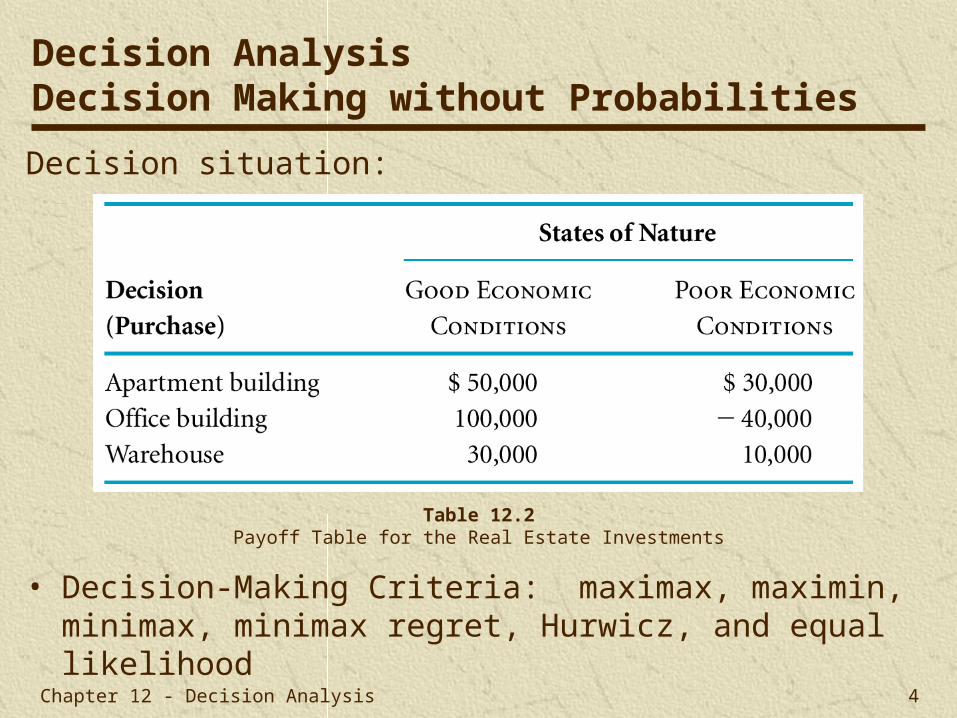
Decision situation:
• Decision-Making Criteria: maximax, maximin, minimax, minimax regret, Hurwicz, and equal likelihood
Table 12.2Payoff Table for the Real Estate Investments
Decision AnalysisDecision Making without Probabilities

Chapter 12 - Decision Analysis 5
Table 12.3Payoff Table Illustrating a Maximax Decision
In the maximax criterion the decision maker selects the decision that will result in the maximum of maximum payoffs; an optimistic criterion.
Decision Making without ProbabilitiesMaximax Criterion

Chapter 12 - Decision Analysis 6
Table 12.4Payoff Table Illustrating a Maximin Decision
In the maximin criterion the decision maker selects the decision that will reflect the maximum of the minimum payoffs; a pessimistic criterion.
Decision Making without ProbabilitiesMaximin Criterion

Chapter 12 - Decision Analysis 7
Table 12.6 Regret Table Illustrating the Minimax Regret Decision
Regret is the difference between the payoff from the best decision and all other decision payoffs.
The decision maker attempts to avoid regret by selecting the decision alternative that minimizes the maximum regret.
Decision Making without ProbabilitiesMinimax Regret Criterion

Chapter 12 - Decision Analysis 8
The Hurwicz criterion is a compromise between the maximax and maximin criterion.
A coefficient of optimism, , is a measure of the decision maker’s optimism.
The Hurwicz criterion multiplies the best payoff by and the worst payoff by 1- ., for each decision, and the best result is selected.
Decision Values
Apartment building $50,000(.4) + 30,000(.6) = 38,000
Office building $100,000(.4) - 40,000(.6) = 16,000
Warehouse $30,000(.4) + 10,000(.6) = 18,000
Decision Making without ProbabilitiesHurwicz Criterion

Chapter 12 - Decision Analysis 9
The equal likelihood ( or Laplace) criterion multiplies the decision payoff for each state of nature by an equal weight, thus assuming that the states of nature are equally likely to occur.
Decision Values
Apartment building $50,000(.5) + 30,000(.5) = 40,000
Office building $100,000(.5) - 40,000(.5) = 30,000
Warehouse $30,000(.5) + 10,000(.5) = 20,000
Decision Making without ProbabilitiesEqual Likelihood Criterion

Chapter 12 - Decision Analysis 10
A dominant decision is one that has a better payoff than another decision under each state of nature.
The appropriate criterion is dependent on the “risk” personality and philosophy of the decision maker.
Criterion Decision (Purchase)
Maximax Office building
Maximin Apartment building
Minimax regret Apartment building
Hurwicz Apartment building
Equal likelihood Apartment building
Decision Making without ProbabilitiesSummary of Criteria Results
Chapter 12 - Decision Analysis 11
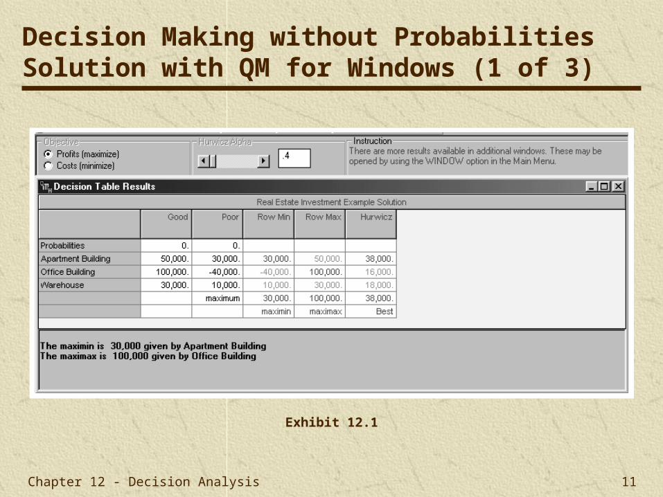
Exhibit 12.1
Decision Making without ProbabilitiesSolution with QM for Windows (1 of 3)
Chapter 12 - Decision Analysis 12
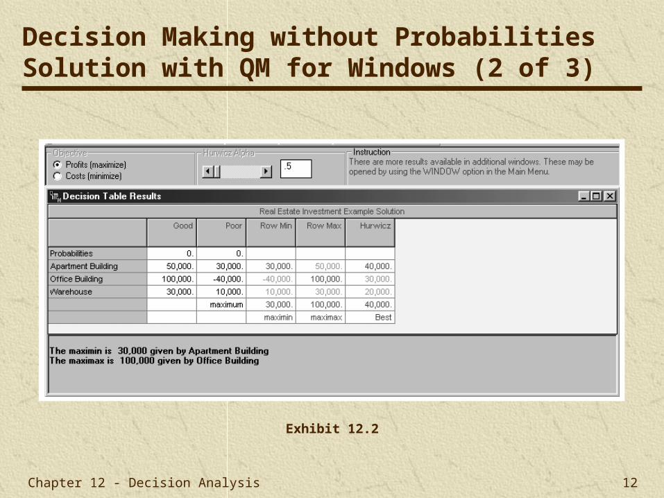
Exhibit 12.2
Decision Making without ProbabilitiesSolution with QM for Windows (2 of 3)

Chapter 12 - Decision Analysis 13
Exhibit 12.3
Decision Making without ProbabilitiesSolution with QM for Windows (3 of 3)
Chapter 12 - Decision Analysis 14
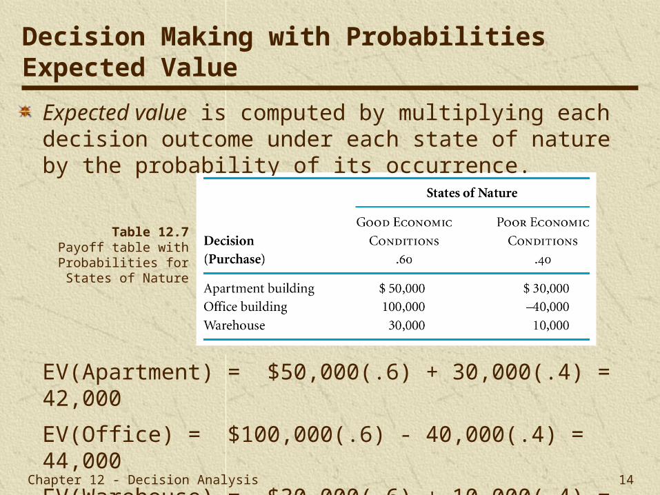
Expected value is computed by multiplying each decision outcome under each state of nature by the probability of its occurrence.
EV(Apartment) = $50,000(.6) + 30,000(.4) = 42,000
EV(Office) = $100,000(.6) - 40,000(.4) = 44,000
EV(Warehouse) = $30,000(.6) + 10,000(.4) = 22,000
Table 12.7Payoff table with
Probabilities for States of Nature
Decision Making with ProbabilitiesExpected Value

Chapter 12 - Decision Analysis 15
The expected opportunity loss is the expected value of the regret for each decision.
The expected value and expected opportunity loss criterion result in the same decision.
EOL(Apartment) = $50,000(.6) + 0(.4) = 30,000
EOL(Office) = $0(.6) + 70,000(.4) = 28,000
EOL(Warehouse) = $70,000(.6) + 20,000(.4) = 50,000
Table 12.8Regret (Opportunity Loss) Table
with Probabilities for States of Nature
Decision Making with ProbabilitiesExpected Opportunity Loss

Chapter 12 - Decision Analysis 16
Exhibit 12.4
Expected Value ProblemsSolution with QM for Windows

Chapter 12 - Decision Analysis 17
Exhibit 12.5
Expected Value ProblemsSolution with Excel and Excel QM (1 of 2)
Chapter 12 - Decision Analysis 18
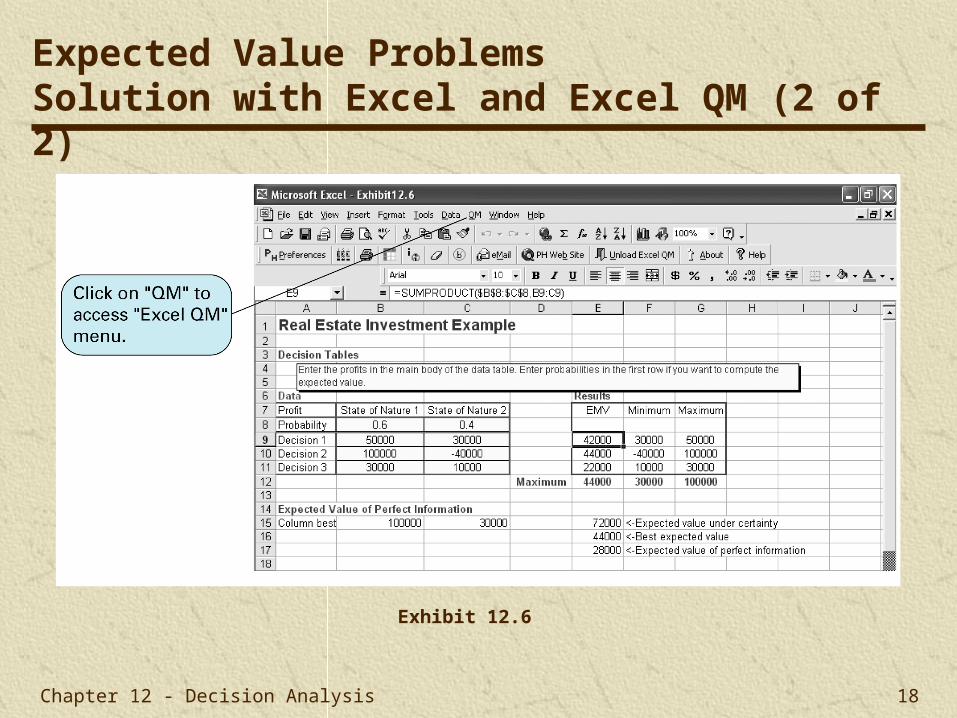
Exhibit 12.6
Expected Value ProblemsSolution with Excel and Excel QM (2 of 2)

Chapter 12 - Decision Analysis 19
The expected value of perfect information (EVPI) is the maximum amount a decision maker would pay for additional information.
EVPI equals the expected value given perfect information minus the expected value without perfect information.
EVPI equals the expected opportunity loss (EOL) for the best decision.
Decision Making with ProbabilitiesExpected Value of Perfect Information

Chapter 12 - Decision Analysis 20
Table 12.9Payoff Table with Decisions, Given Perfect Information
Decision Making with ProbabilitiesEVPI Example (1 of 2)
Chapter 12 - Decision Analysis 21
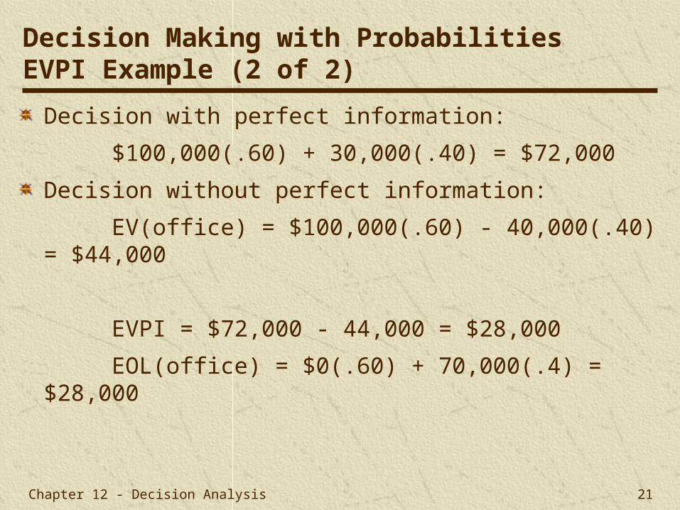
Decision with perfect information:
$100,000(.60) + 30,000(.40) = $72,000
Decision without perfect information:
EV(office) = $100,000(.60) - 40,000(.40) = $44,000
EVPI = $72,000 - 44,000 = $28,000
EOL(office) = $0(.60) + 70,000(.4) = $28,000
Decision Making with ProbabilitiesEVPI Example (2 of 2)

Chapter 12 - Decision Analysis 22
Exhibit 12.7
Decision Making with ProbabilitiesEVPI with QM for Windows

Chapter 12 - Decision Analysis 23
A decision tree is a diagram consisting of decision nodes (represented as squares), probability nodes (circles), and decision alternatives (branches).
Table 12.10Payoff Table for Real Estate Investment Example
Decision Making with ProbabilitiesDecision Trees (1 of 4)

Chapter 12 - Decision Analysis 24
Figure 12.1Decision Tree for Real Estate Investment Example
Decision Making with ProbabilitiesDecision Trees (2 of 4)
Chapter 12 - Decision Analysis 25
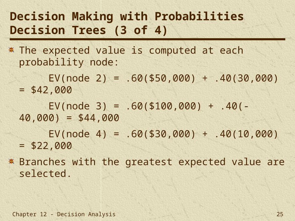
The expected value is computed at each probability node:
EV(node 2) = .60($50,000) + .40(30,000) = $42,000
EV(node 3) = .60($100,000) + .40(-40,000) = $44,000
EV(node 4) = .60($30,000) + .40(10,000) = $22,000
Branches with the greatest expected value are selected.
Decision Making with ProbabilitiesDecision Trees (3 of 4)

Chapter 12 - Decision Analysis 26
Figure 12.2Decision Tree with Expected Value at Probability Nodes
Decision Making with ProbabilitiesDecision Trees (4 of 4)

Chapter 12 - Decision Analysis 27
Exhibit 12.8
Decision Making with ProbabilitiesDecision Trees with QM for Windows
Chapter 12 - Decision Analysis 28
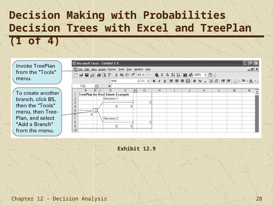
Exhibit 12.9
Decision Making with ProbabilitiesDecision Trees with Excel and TreePlan (1 of 4)

Chapter 12 - Decision Analysis 29
Exhibit 12.10
Decision Making with ProbabilitiesDecision Trees with Excel and TreePlan (2 of 4)

Chapter 12 - Decision Analysis 30
Exhibit 12.11
Decision Making with ProbabilitiesDecision Trees with Excel and TreePlan (3 of 4)
Chapter 12 - Decision Analysis 31
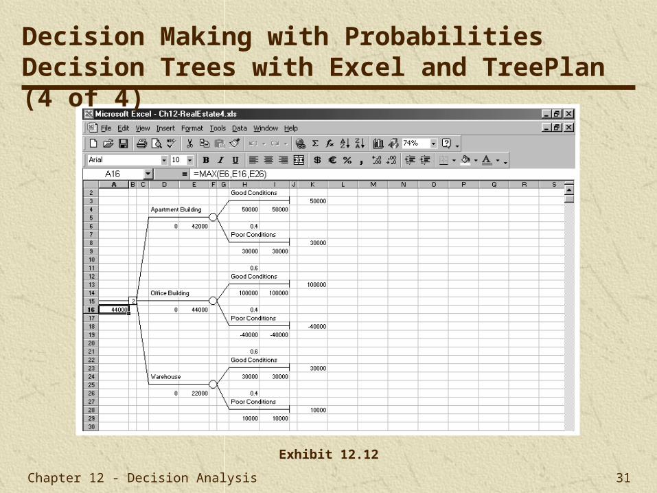
Exhibit 12.12
Decision Making with ProbabilitiesDecision Trees with Excel and TreePlan (4 of 4)

Chapter 12 - Decision Analysis 32
Decision Making with ProbabilitiesSequential Decision Trees (1 of 4)
A sequential decision tree is used to illustrate a situation requiring a series of decisions.
Used where a payoff table, limited to a single decision, cannot be used.
Real estate investment example modified to encompass a ten-year period in which several decisions must be made:

Chapter 12 - Decision Analysis 33
Figure 12.3Sequential Decision Tree
Decision Making with ProbabilitiesSequential Decision Trees (2 of 4)
Chapter 12 - Decision Analysis 34
Decision Making with ProbabilitiesSequential Decision Trees (3 of 4)
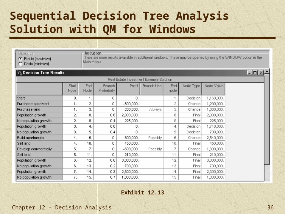
Decision is to purchase land; highest net expected value ($1,160,000).
Payoff of the decision is $1,160,000.
Chapter 12 - Decision Analysis 35
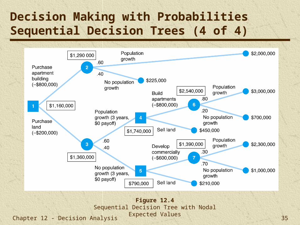
Figure 12.4Sequential Decision Tree with Nodal Expected Values
Decision Making with ProbabilitiesSequential Decision Trees (4 of 4)
Chapter 12 - Decision Analysis 36
Exhibit 12.13
Sequential Decision Tree AnalysisSolution with QM for Windows

Chapter 12 - Decision Analysis 37
Exhibit 12.14
Sequential Decision Tree AnalysisSolution with Excel and TreePlan

Chapter 12 - Decision Analysis 38
Bayesian analysis uses additional information to alter the marginal probability of the occurrence of an event.
In real estate investment example, using expected value criterion, best decision was to purchase office building with expected value of $444,000, and EVPI of $28,000.
Table 12.11Payoff Table for the Real Estate Investment Example
Decision Analysis with Additional InformationBayesian Analysis (1 of 3)

Chapter 12 - Decision Analysis 39
A conditional probability is the probability that an event will occur given that another event has already occurred.
Economic analyst provides additional information for real estate investment decision, forming conditional probabilities:
g = good economic conditions
p = poor economic conditions
P = positive economic report
N = negative economic report
P(Pg) = .80 P(NG) = .20
P(Pp) = .10 P(Np) = .90
Decision Analysis with Additional InformationBayesian Analysis (2 of 3)
Chapter 12 - Decision Analysis 40
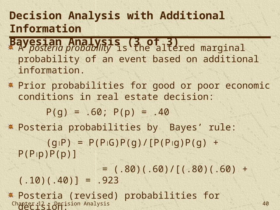
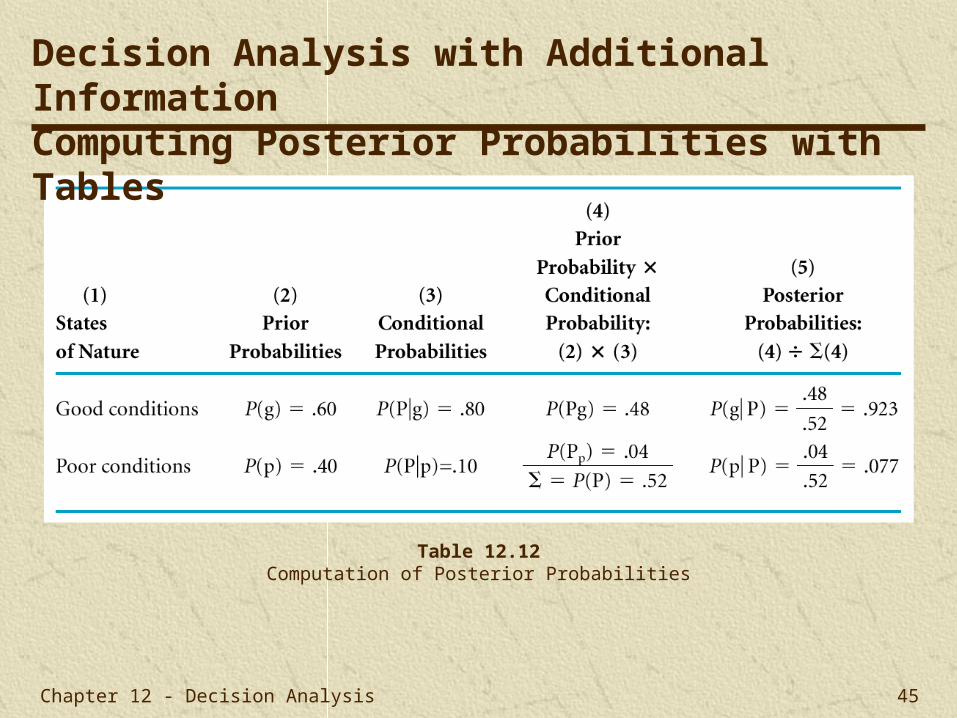
A posteria probability is the altered marginal probability of an event based on additional information.
Prior probabilities for good or poor economic conditions in real estate decision:
P(g) = .60; P(p) = .40
Posteria probabilities by Bayes’ rule:
(gP) = P(PG)P(g)/[P(Pg)P(g) + P(Pp)P(p)]
= (.80)(.60)/[(.80)(.60) + (.10)(.40)] = .923
Posteria (revised) probabilities for decision:
P(gN) = .250 P(pP) = .077 P(pN) = .750
Decision Analysis with Additional InformationBayesian Analysis (3 of 3)

Chapter 12 - Decision Analysis 41
Decision Analysis with Additional InformationDecision Trees with Posterior Probabilities (1 of 4)
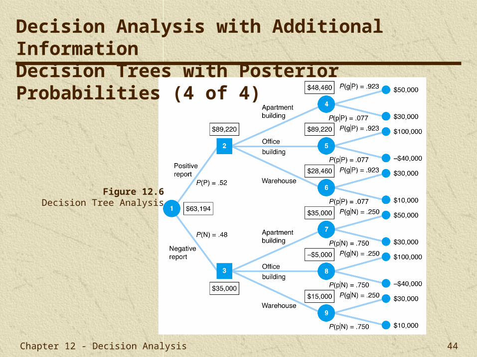
Decision tree with posterior probabilities differ from earlier versions in that:
Two new branches at beginning of tree represent report outcomes.
Probabilities of each state of nature are posterior probabilities from Bayes’ rule.

Chapter 12 - Decision Analysis 42
Figure 12.5Decision Tree with
Posterior Probabilities
Decision Analysis with Additional InformationDecision Trees with Posterior Probabilities (2 of 4)
Chapter 12 - Decision Analysis 43
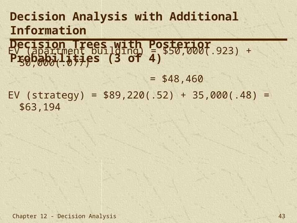
Decision Analysis with Additional InformationDecision Trees with Posterior Probabilities (3 of 4)
EV (apartment building) = $50,000(.923) + 30,000(.077)
= $48,460
EV (strategy) = $89,220(.52) + 35,000(.48) = $63,194
Chapter 12 - Decision Analysis 44
Figure 12.6Decision Tree Analysis
Decision Analysis with Additional InformationDecision Trees with Posterior Probabilities (4 of 4)
Chapter 12 - Decision Analysis 45
Table 12.12Computation of Posterior Probabilities
Decision Analysis with Additional InformationComputing Posterior Probabilities with Tables

Chapter 12 - Decision Analysis 46
The expected value of sample information (EVSI) is the difference between the expected value with and without information:
For example problem, EVSI = $63,194 - 44,000 = $19,194
The efficiency of sample information is the ratio of the expected value of sample information to the expected value of perfect information:
efficiency = EVSI /EVPI = $19,194/ 28,000 = .68
Decision Analysis with Additional InformationExpected Value of Sample Information
Chapter 12 - Decision Analysis 47
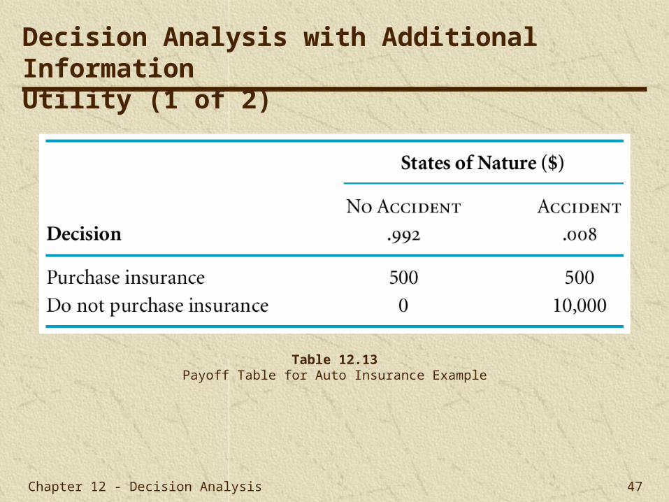
Table 12.13Payoff Table for Auto Insurance Example
Decision Analysis with Additional InformationUtility (1 of 2)
Chapter 12 - Decision Analysis 48
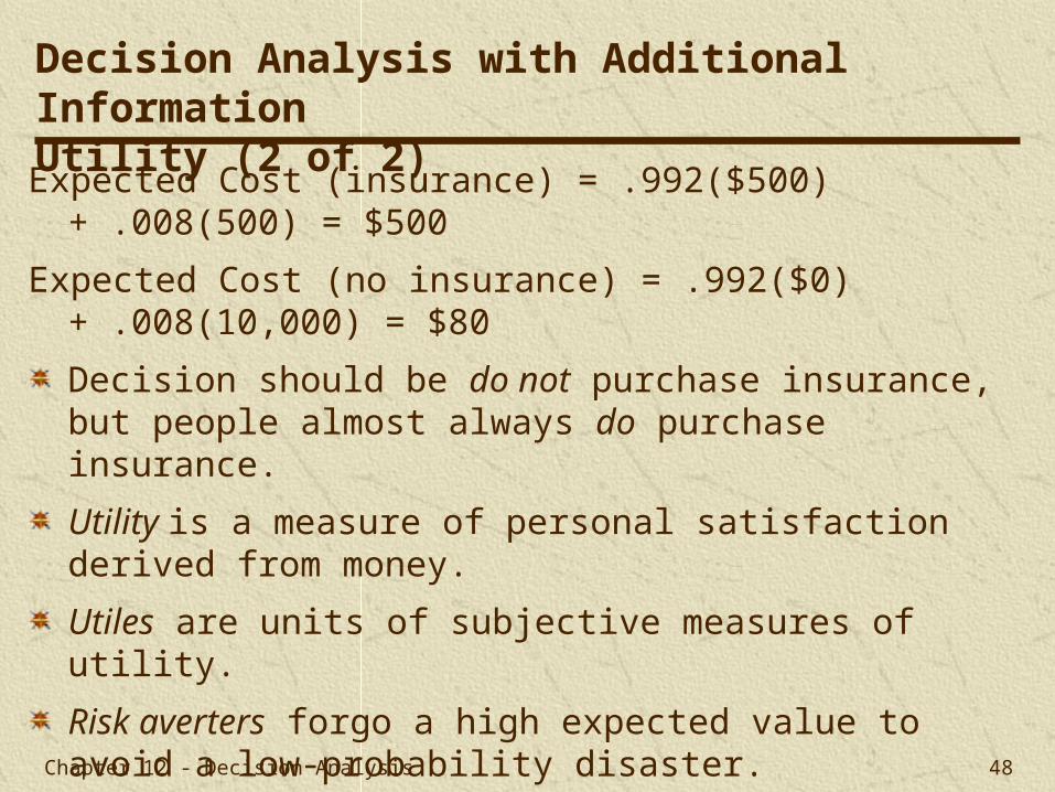
Expected Cost (insurance) = .992($500) + .008(500) = $500
Expected Cost (no insurance) = .992($0) + .008(10,000) = $80
Decision should be do not purchase insurance, but people almost always do purchase insurance.
Utility is a measure of personal satisfaction derived from money.
Utiles are units of subjective measures of utility.
Risk averters forgo a high expected value to avoid a low-probability disaster.
Risk takers take a chance for a bonanza on a very low-probability event in lieu of a sure thing.
Decision Analysis with Additional InformationUtility (2 of 2)

Chapter 12 - Decision Analysis 49
States of Nature
Decision Good Foreign
Competitive Conditions Poor Foreign Competitive
Conditions
Expand Maintain Status Quo Sell now
$ 800,000 1,300,000 320,000
$ 500,000 -150,000 320,000
Decision Analysis Example Problem Solution (1 of 9)

Chapter 12 - Decision Analysis 50
Decision Analysis Example Problem Solution (2 of 9)
a. Determine the best decision without probabilities using the 5 criteria of the chapter.
b. Determine best decision with probabilities assuming .70 probability of good conditions, .30 of poor conditions. Use expected value and expected opportunity loss criteria.
c. Compute expected value of perfect information.
d. Develop a decision tree with expected value at the nodes.
e. Given following, P(Pg) = .70, P(Ng) = .30, P(Pp) = 20, P(Np) = .80, determine posteria probabilities using Bayes’ rule.
f. Perform a decision tree analysis using the posterior probability obtained in part e.

Chapter 12 - Decision Analysis 51
Step 1 (part a): Determine decisions without probabilities.
Maximax Decision: Maintain status quo
Decisions Maximum Payoffs
Expand $800,000Status quo 1,300,000 (maximum)Sell 320,000
Maximin Decision: Expand
Decisions Minimum Payoffs
Expand $500,000 (maximum)Status quo -150,000Sell 320,000
Decision Analysis Example Problem Solution (3 of 9)

Chapter 12 - Decision Analysis 52
Minimax Regret Decision: Expand
Decisions Maximum Regrets
Expand $500,000 (minimum)
Status quo 650,000
Sell 980,000
Hurwicz ( = .3) Decision: Expand
Expand $800,000(.3) + 500,000(.7) = $590,000
Status quo $1,300,000(.3) - 150,000(.7) = $285,000
Sell $320,000(.3) + 320,000(.7) = $320,000
Decision Analysis Example Problem Solution (4 of 9)

Chapter 12 - Decision Analysis 53
Equal Likelihood Decision: Expand
Expand $800,000(.5) + 500,000(.5) = $650,000
Status quo $1,300,000(.5) - 150,000(.5) = $575,000
Sell $320,000(.5) + 320,000(.5) = $320,000
Step 2 (part b): Determine Decisions with EV and EOL.
Expected value decision: Maintain status quo
Expand $800,000(.7) + 500,000(.3) = $710,000
Status quo $1,300,000(.7) - 150,000(.3) = $865,000
Sell $320,000(.7) + 320,000(.3) = $320,000
Decision Analysis Example Problem Solution (5 of 9)
Chapter 12 - Decision Analysis 54
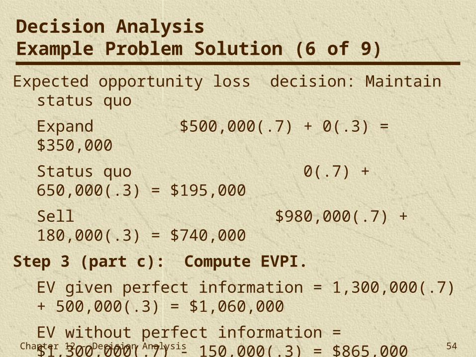
Expected opportunity loss decision: Maintain status quo
Expand $500,000(.7) + 0(.3) = $350,000
Status quo 0(.7) + 650,000(.3) = $195,000
Sell $980,000(.7) + 180,000(.3) = $740,000
Step 3 (part c): Compute EVPI.
EV given perfect information = 1,300,000(.7) + 500,000(.3) = $1,060,000
EV without perfect information = $1,300,000(.7) - 150,000(.3) = $865,000
EVPI = $1.060,000 - 865,000 = $195,000
Decision Analysis Example Problem Solution (6 of 9)

Chapter 12 - Decision Analysis 55
Step 4 (part d): Develop a decision tree.
Decision Analysis Example Problem Solution (7 of 9)

Chapter 12 - Decision Analysis 56
Step 5 (part e): Determine posterior probabilities.
P(gP) = P(PG)P(g)/[P(Pg)P(g) + P(Pp)P(p)]
= (.70)(.70)/[(.70)(.70) + (.20)(.30)] = .891
P(pP) = .109
P(gN) = P(NG)P(g)/[P(Ng)P(g) + P(Np)P(p)]
= (.30)(.70)/[(.30)(.70) + (.80)(.30)] = .467
P(pN) = .533
Decision Analysis Example Problem Solution (8 of 9)

Chapter 12 - Decision Analysis 57
Step 6 (part f): Decision tree analysis.
Decision Analysis Example Problem Solution (9 of 9)
Related Documents


