Chapter 11 Waves and Imaging We now return to those thrilling days of waves to consider their effects on the per- formance of imaging systems. We first consider “interference” of two traveling waves that oscillate with the same frequency and then generalize that to the interference of many such waves, which is called “diffraction”. 11.1 Interference of Waves References: Hecht, Optics §8 Recall the identity that was derived for the sum of two oscillations with different frequencies ω 1 and ω 2 : y 1 [t]= A cos [ω 1 t] y 2 [t]= A cos [ω 2 t] y 1 [t]+ y 2 [t]=2A cos ∙μ ω 1 + ω 2 2 ¶ t ¸ · cos ∙μ ω 1 − ω 2 2 ¶ t ¸ ≡ 2A cos [ω avg t] · cos [ω mod t] In words, the sum of two oscillations of different frequency is identical to the product of two oscillations: one is the slower varying modulation (at frequency ω mod ) and the other is the more rapidly oscillating average sinusoid (or carrier wave) with frequency ω avg . A perhaps familiar example of the modulation results from the excitation of two piano strings that are mistuned. A low-frequency oscillation (the beat) is heard; as one string is tuned to the other, the frequency of the beat decreases, reaching zero when the string frequencies are equal. Acoustic beats may be thought of as interference of the summed oscillations in time. We also could consider this relationship in a broader sense. If the sinusoids are considered to be functions of the independent variable (coordinate) t, the phase angles of the two component functions Φ 1 (t)= ω 1 t and Φ 2 (t)= ω 2 t are different at the same coordinate t. The components sometimes add (for t such that Φ 1 [t] ∼ = Φ 2 [t] ± 2nπ) and sometimes subtract (if Φ 1 (t) ∼ = Φ 2 (t) ± (2n + 1)π). 219

Welcome message from author
This document is posted to help you gain knowledge. Please leave a comment to let me know what you think about it! Share it to your friends and learn new things together.
Transcript
Chapter 11
Waves and Imaging
We now return to those thrilling days of waves to consider their effects on the per-formance of imaging systems. We first consider “interference” of two traveling wavesthat oscillate with the same frequency and then generalize that to the interference ofmany such waves, which is called “diffraction”.
11.1 Interference of Waves
References: Hecht, Optics §8Recall the identity that was derived for the sum of two oscillations with different
frequencies ω1 and ω2 :
y1 [t] = A cos [ω1t]
y2 [t] = A cos [ω2t]
y1 [t] + y2 [t] = 2A cos
∙µω1 + ω22
¶t
¸· cos
∙µω1 − ω22
¶t
¸≡ 2A cos [ωavgt] · cos [ωmodt]
In words, the sum of two oscillations of different frequency is identical to the productof two oscillations: one is the slower varying modulation (at frequency ωmod) and theother is the more rapidly oscillating average sinusoid (or carrier wave) with frequencyωavg . A perhaps familiar example of the modulation results from the excitation oftwo piano strings that are mistuned. A low-frequency oscillation (the beat) is heard;as one string is tuned to the other, the frequency of the beat decreases, reachingzero when the string frequencies are equal. Acoustic beats may be thought of asinterference of the summed oscillations in time.We also could consider this relationship in a broader sense. If the sinusoids are
considered to be functions of the independent variable (coordinate) t, the phase anglesof the two component functions Φ1(t) = ω1t and Φ2(t) = ω2t are different at the samecoordinate t. The components sometimes add (for t such that Φ1 [t] ∼= Φ2 [t] ± 2nπ)and sometimes subtract (if Φ1(t) ∼= Φ2(t)± (2n+ 1)π).
219

220 CHAPTER 11 WAVES AND IMAGING
We also derived the analogous effect for two waves traveling along the z -axis:
f1 [z, t] = A cos [k1z − ω1t]
f2 [z, t] = A cos [k2z − ω2t]
f1 [z, t] + f2 [z, t] = {2A cos[kmodz − ωmodt]} · cos[kavgz − ωavgt]
kmod =k1 − k22
ωmod =ω1 − ω22
vmod =ωmodkmod
=ω1 − ω2k1 − k2
kavg =k1 + k22
ωavg =ω1 + ω22
vavg =ωavgkavg
=ω1 + ω2k1 + k2
In words, the superposition of two traveling waves with different temporal frequencies(and thus different wavelengths) generates the product of two component travelingwaves, one oscillating more slowly in both time and space,i.e. a traveling modulation.Note that both the average and modulation waves move along the z-axis. In thiscase,k1, k2, ω1,and ω2are all positive, and so kavg and ωavg must be also. However, themodulation wavenumber and frequency may be negative. In fact, the algebraic signof kmod may be negative even if ωmod is positive. In this case, the modulation wavemoves in the opposite direction to the average wave.
Note that if the two 1-D waves traveling in the same direction along the z-axishave the same frequency ω, they must have the same wavelength λ and the samewavenumber k = 2π
λ. The modulation terms kmod and ωmod must be zero, and the
summation wave exhibits no modulation. Recall also such waves traveling in oppositedirections generate a waveform that moves but does not travel, but is a standing wave:
f1 [z, t] = A cos [k1z − ω1t]
f2 [z, t] = A cos [k1z + ω1t]
f1 [z, t] + f2 [z, t] = {2A cos [kmodz − ωmodt]} cos [kavgz − ωavgt]

11.1 INTERFERENCE OF WAVES 221
kmod =k1 − k12
= 0
ωmod =ω1 − (−ω1)
2= ω1
kavg =k1 + k12
= k1
ωavg =ω1 + (−ω1)
2= 0
f1 [z, t] + f2 [z, t] = 2A cos [k1z] cos [−ω1t]= 2A cos [k1z] cos [ω1t]
where the symmetry of cos[θ] was used in the last step.
Traveling waves also may be defined over two or three spatial dimensions; thewaves have the form f [x, y, t] and f [x, y, z, t], respectively. The direction of propaga-tion of such a wave in a multidimensional space is determined by a vector analogousto k; a 3-D wavevector k has components [kx, ky, kz]. The vector may be written:
k =£kxx+ kyy + kzz
¤The corresponding wave travels in the direction of the wavevector k and has wave-length λ = 2π
|k| . In other words, the length of k is the magnitude of the wavevector:
|k| =qk2x + k2y + k2z =
2π
λ.
The temporal oscillation frequency ω is determined from the magnitude of the wavevec-tor through the dispersion relation:
ω = vφ · |k|→ ν =vφλ
For illustration, consider a simple 2-D analogue of the 1-D traveling plane wave.The wave travels in the direction of the 2-D wavevector k which is in the x− z plane:
k = [kx, 0, kz]
The points of constant phase with with phase angle φ = C radians is the set of pointsin the 2-D space r = [x = 0, y, z] = (r, θ) such that the scalar product k · r = C:

222 CHAPTER 11 WAVES AND IMAGING
k • r = r • k= |k||r| cos [θ]= kxx+ kzz = C for a point of constant phase
Therefore, the equation of a 2-D wave traveling in the direction of k with linearwavefronts is:
f [x, y, t] = A cos [kxx+ kzz − ωt]
= A cos [k • r− ωt]
In three dimensions, the set of points with the same phase lie on a planar surface sothat the equation of the traveling wave is:
f [x, y, z, t] = f [r, t]
= A cos [kxx+ kyy + kzz − ωt]
= A cos [k • r− ωt]
Plane wave traveling in direction k
This plane wave could have been created by a point source at a large distance to theleft and below the z-axis.
Now, we will apply the equation derived when adding oscillations with different
11.1 INTERFERENCE OF WAVES 223
temporal frequencies. In general, the form of the sum of two traveling waves is:
f1 [x, y, z, t] + f2 [x, y, z, t] = A cos [k1•r− ωt] +A cos [k2•r− ωt]
= 2A cos£kavg · r− ωavgt
¤· cos [kmod•r− ωmodt]
where the average and modulation wavevectors are:
kavg =k1 + k22
=(kx)1 + (kx)2
2x+
(ky)1 + (ky)22
y+(kz)1 + (kz)2
2z
kmod =k1 − k22
=(kx)1 − (kx)2
2x+
(ky)1 − (ky)22
y +(kz)1 − (kz)2
2z
and the average and modulation angular temporal frequencies are:
ωavg =ω1 + ω22
ωmod =ω1 − ω22
Note that the average and modulation wavevectors kavg and kmod point in differentdirections, in general, and thus the corresponding waves move in different directionsat velocities determined from:
vavg =ωavg|kavg|
vmod =ωmod|kmod|
Because the phase of the multidimensional traveling wave is a function of twoparameters (the wavevector k and the angular temporal frequency ω), the phases oftwo traveling waves usually differ even if the temporal frequencies are equal. Considerthe superposition of two such waves:
ω1 = ω2 ≡ ω
The component waves travel in different directions so the components of the wavevec-tors differ:
k1 = [(kx)1, (ky)1, (kz)1] 6= k2 = [(kx)2, (ky)2, (kz)2]Since the temporal frequencies are equal, so must be the wavelengths:
λ1 = λ2 = λ→ |k1| = |k2| ≡ |k| .
The condition of equal ω ensures that the temporal average and modulation frequen-
224 CHAPTER 11 WAVES AND IMAGING
cies are:
ωavg =ω1 + ω22
= ω0
ωmod =ω1 − ω22
= 0
The summation of the two traveling waves with identical magnitudes may beexpressed as:
f1[x, y, z, t] + f21[x, y, z, t] = A cos(k1•r− ω0t) +A cos(k2•r− ω0t)
= 2A cos(kavg • r− ωavgt) · cos(kmod • r− 0 · t)= 2A cos(kavg • r− ωavgt) · cos(kmod • r)
Therefore, the superposition of two 2-D wavefronts with the same temporal frequencybut traveling in different directions results in two multiplicative components: a trav-eling wave in the direction of kavg, and a wave in space along the direction of kmodthat does not move. This second stationary wave is analogous to the phenomenon ofbeats, and is called interference in optics.
11.1.1 Superposition of Two Plane Waves of the Same Fre-quency
Consider the superposition of two plane waves:
f1 [x, y, z, t] = A cos [k1 • r− ω0t]
f2 [x, y, z, t] = A cos [k2 • r− ω0t]
k1 = [kx, ky = 0, kz]
k2 = [−kx, 0, kz]
i.e., the wavevectors differ only in the x -component, and there only by a sign. There-fore the two wavevectors have the same “length”:
|k1| = |k2| =2π
λ=⇒ λ1 = λ2 ≡ λ.
Also note that:
kz = |k| cos [θ] =2π
λcos [θ]
kx =2π
λsin [θ]
11.1 INTERFERENCE OF WAVES 225
kavg =k1 + k22
=[kx, 0, kz] + [kx, 0, kz]
2= [0, 0, kz] = z
2π
λcos [θ]
kavg =k1 − k22
=[kx, 0, kz] + [−kx, 0, kz]
2= [kx, 0, 0] = x
2π
λsin [θ]
ωavg =ω1 + ω22
= ω0
ωmod =ω1 − ω22
= 0
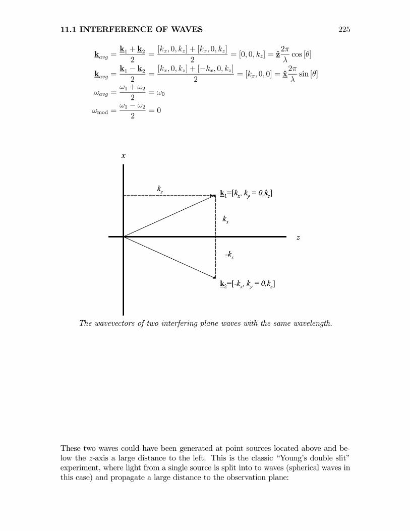
The wavevectors of two interfering plane waves with the same wavelength.
These two waves could have been generated at point sources located above and be-low the z-axis a large distance to the left. This is the classic “Young’s double slit”experiment, where light from a single source is split into to waves (spherical waves inthis case) and propagate a large distance to the observation plane:

226 CHAPTER 11 WAVES AND IMAGING
How two “tilted” plane waves are generated in the Young double-apertureexperiment. The two apertures in the opaque screen on the left divide the incomingwave into two expanding spherical waves. After propagating a long distance, thespherical waves approximate plane waves that are tilted relative to the axis by
θ = d2·L .
The “tilts” of the two waves are evaluated from the two distances:
θ ∼= d/2
L=
d
2L
If L >> d, then
θ ∼= tan [θ] ∼= sin [θ] ∼= d
2L
The superposition of the two electric fields is:
f [x, y, z, t] = f1[x, y, z, t] + f2[x, y, z, t]
= 2A cos£kavg • r− ωavgt
¤· cos [kmod • r]
= 2A cosh2π
z
λcos [θ]− ω0t
icosh2π
x
λsin [θ]
iThe first term (with the time dependence) is a traveling wave in the direction definedby k = [0, 0, kz], while the second term (with no dependence on time) is a spatial

11.1 INTERFERENCE OF WAVES 227
wave along the y direction. The amplitude variation in the y direction is:
2A cosh2π
y
λsin [θ]
i= 2A cos
⎡⎣2π x³λ
sin[θ]
´⎤⎦
which has a period of λsin[θ]
. The irradiance (the measureable intensity) of the super-position is:
|f [x, y, z, t] |2 = 4A2 cos2h2π
z
λcos [θ]− ω0t
icos2
∙2πx sin [θ]
λ
¸The second cosine terms can be rewritten using:
cos2 [θ] =1
2(1 + cos [2θ])
As before, the first term varies rapidly due to the angular frequency term ω0 ∼= 1014Hz.Therefore, just the average value is detected:
|f [x, y, z, t] |2
®= 4A2 cos2
∙2πx sin [θ]
λ
¸· 12
= 2A2∙1
2
µ1 + cos
∙4πx sin [θ]
λ
¸¶¸
= A2
⎛⎝1 + cos⎡⎣2π x³
λ2·sin[θ]
´⎤⎦⎞⎠
This derivation may also be applied to find the irradiance of one of the individualcomponent waves:
I1 =|f1 [x, y, z, t]|2
®I2 =
|f2 [x, y, z, t]|2
®I0 =
|f1 [x, y, z, t]|2
®=|A cos [k1 · r− ω0t]|2
®= A2
cos2 [k1 · r− ω0t]
®= A2 · 1
2

228 CHAPTER 11 WAVES AND IMAGING
So the irradiance of the sum of the two waves can be rewritten in terms of theirradiance of a single wave:
|f [x, y, z, t] |2
®= 4I0 cos
2
∙2πx sin [θ]
λ
¸= 2I0
µ1 +
cos [2πx · 2 · sin [θ]]λ
¶
= 2I0
⎛⎝1 + cos⎡⎣2π x³
λ2 sin[θ]
´⎤⎦⎞⎠
The irradiance exhibits a sinusoidal modulation of periodX = λ2 sin[θ]
and its irradianceoscillates between 0 and 2I0 · (2) = 4I0, so that the average irradiance is 2I0. Theperiod varies directly with λ and inversely with sin(θ); for small θ, the period of thesinusoid is large, for θ = 0, there is no modulation of the irradiance. The alternatingbright and dark regions of this time-stationary sinusoidal intensity pattern often arecalled interference fringes. The shape, separation, and orientation of the interferencefringes are determined by the incident wavefronts, and thus provide information aboutthem. The argument of the cosine function is the optical phase difference of the twowaves. At locations where the optical phase difference is an even multiple of π, thecosine evaluates to unity and a maximum of the interference pattern results. Thisis an example of constructive interference. If the optical phase difference is an oddmultiple of π, the cosine evaluates to -1 and the irradiance is zero; this is destructiveinterference.
Interference of two “tilted plane waves” with the same wavelength. The twocomponent traveling waves are shown as “snapshots” at one instant of time on the

11.1 INTERFERENCE OF WAVES 229
left (white = 1, black = -1); the sum of the two is shown in the center (white = 2,black = -2), and the squared magnitude on the right (white = 4, blace = 0). The
modulation in the vertical direction is constant, while that in the horizontal directionis a traveling wave and “averages” out to a constant value of 1
2.
The amplitude and irradiance observed at one instant of time when the irradiance atthe origin (“on axis”) is a maximum is shown:
Interference patterns observed along the x-axis at one value of z: (a) amplitudefringes, with period equal to λ
sin[θ]; irradiance (intensity) fringes, with period equal to
λ2·sin[θ] . This pattern is averaged over time and scales by a factor of
12.
Again, the traveling wave in the images of the amplitude and intensity of thesuperposed images moves in the z-direction (to the right), thus blurring out theoscillations in the z-direction. The oscillations in the x-direction are preserved as theinterference pattern, which is plotted as a function of x below. Note that the spatialfrequency of the intensity fringes is twice as large as that of the amplitude fringes.
Irradiance patterns observed at the output plane at several instants of time, showingthat the spatial variation of the irradiance is preserved but the averaging reduces the
maximum value by half.
230 CHAPTER 11 WAVES AND IMAGING
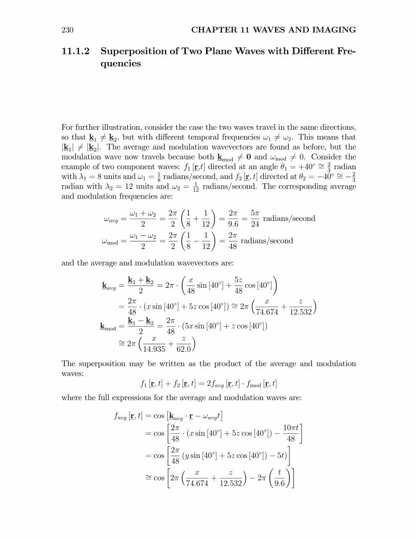
11.1.2 Superposition of Two PlaneWaves with Different Fre-quencies
For further illustration, consider the case the two waves travel in the same directions,so that k1 6= k2, but with different temporal frequencies ω1 6= ω2. This means that|k1| 6= |k2|. The average and modulation wavevectors are found as before, but themodulation wave now travels because both kmod 6= 0 and ωmod 6= 0. Consider theexample of two component waves: f1 [r,t] directed at an angle θ1 = +40◦ ∼= 2
3radian
with λ1 = 8 units and ω1 = 18radians/second, and f2 [r, t] directed at θ2 = −40◦ ∼= −23
radian with λ2 = 12 units and ω2 =112radians/second. The corresponding average
and modulation frequencies are:
ωavg =ω1 + ω22
=2π
2
µ1
8+1
12
¶=2π
9.6=5π
24radians/second
ωmod =ω1 − ω22
=2π
2
µ1
8− 1
12
¶=2π
48radians/second
and the average and modulation wavevectors are:
kavg =k1 + k22
= 2π ·µx
48sin [40◦] +
5z
48cos [40◦]
¶=2π
48· (x sin [40◦] + 5z cos [40◦]) ∼= 2π
³ x
74.674+
z
12.532
´kmod =
k1 − k22
=2π
48· (5x sin [40◦] + z cos [40◦])
∼= 2π³ x
14.935+
z
62.0
´The superposition may be written as the product of the average and modulationwaves:
f1 [r, t] + f2 [r, t] = 2favg [r, t] · fmod [r, t]where the full expressions for the average and modulation waves are:
favg [r, t] = cos£kavg · r− ωavgt
¤= cos
∙2π
48· (x sin [40◦] + 5z cos [40◦])− 10πt
48
¸= cos
∙2π
48(y sin [40◦] + 5z cos [40◦])− 5t)
¸∼= cos
∙2π³ x
74.674+
z
12.532
´− 2π
µt
9.6
¶¸
11.1 INTERFERENCE OF WAVES 231
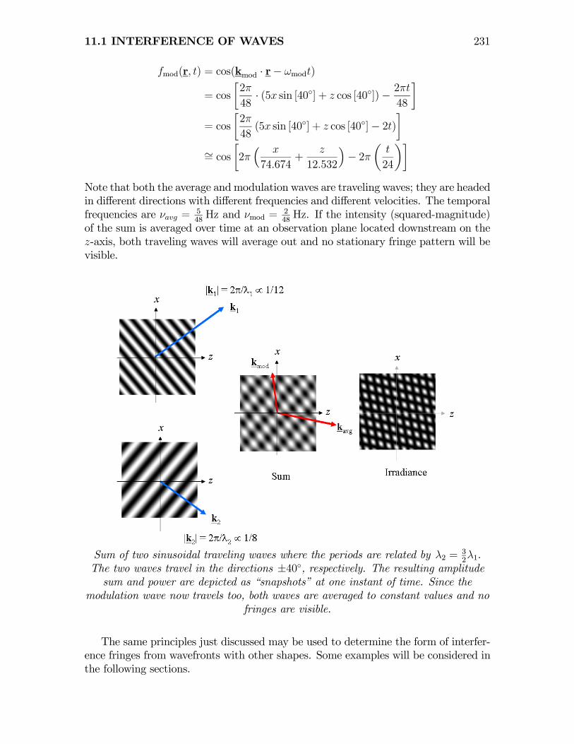
fmod(r, t) = cos(kmod · r− ωmodt)
= cos
∙2π
48· (5x sin [40◦] + z cos [40◦])− 2πt
48
¸= cos
∙2π
48(5x sin [40◦] + z cos [40◦]− 2t)
¸∼= cos
∙2π³ x
74.674+
z
12.532
´− 2π
µt
24
¶¸Note that both the average and modulation waves are traveling waves; they are headedin different directions with different frequencies and different velocities. The temporalfrequencies are νavg = 5
48Hz and νmod =
248Hz. If the intensity (squared-magnitude)
of the sum is averaged over time at an observation plane located downstream on thez-axis, both traveling waves will average out and no stationary fringe pattern will bevisible.
Sum of two sinusoidal traveling waves where the periods are related by λ2 =32λ1.
The two waves travel in the directions ±40◦, respectively. The resulting amplitudesum and power are depicted as “snapshots” at one instant of time. Since the
modulation wave now travels too, both waves are averaged to constant values and nofringes are visible.
The same principles just discussed may be used to determine the form of interfer-ence fringes from wavefronts with other shapes. Some examples will be considered inthe following sections.
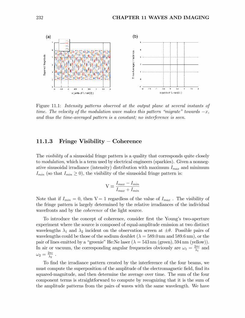
232 CHAPTER 11 WAVES AND IMAGING
Figure 11.1: Intensity patterns observed at the output plane at several instants oftime. The velocity of the modulation wave makes this pattern “migrate” towards −x,and thus the time-averaged pattern is a constant; no interference is seen.
11.1.3 Fringe Visibility — Coherence
The visibility of a sinusoidal fringe pattern is a quality that corresponds quite closelytomodulation, which is a term used by electrical engineers (sparkies). Given a nonneg-ative sinusoidal irradiance (intensity) distribution with maximum Imax and minimumImin (so that Imin ≥ 0), the visibility of the sinusoidal fringe pattern is:
V ≡ Imax − Imin
Imax + Imin
Note that if Imin = 0, then V= 1 regardless of the value of Imax . The visibility ofthe fringe pattern is largely determined by the relative irradiances of the individualwavefronts and by the coherence of the light source.
To introduce the concept of coherence, consider first the Young’s two-apertureexperiment where the source is composed of equal-amplitude emission at two distinctwavelengths λ1 and λ2 incident on the observation screen at ±θ. Possible pairs ofwavelengths could be those of the sodium doublet (λ = 589.0 nm and 589.6 nm), or thepair of lines emitted by a “greenie” He:Ne laser (λ = 543nm (green), 594 nm (yellow)).In air or vacuum, the corresponding angular frequencies obviously are ω1 = 2πc
λ1and
ω2 =2πcλ2.
To find the irradiance pattern created by the interference of the four beams, wemust compute the superposition of the amplitude of the electromagnetic field, find itssquared-magnitude, and then determine the average over time. The sum of the fourcomponent terms is straightforward to compute by recognizing that it is the sum ofthe amplitude patterns from the pairs of waves with the same wavelength. We have

11.1 INTERFERENCE OF WAVES 233
already shown that the sum of the two terms with λ = λ1 is:
f1 [x, z;λ1] + f2 [x, z;λ1] = 2A cos
∙2πx
λ1sin [θ]
¸cos
∙2πz
λ1cos [θ]− ω1t
¸
= 2A cos
⎡⎣2π x³λ1sin[θ]
´⎤⎦ cos ∙2πz
λ1cos [θ]− ω1t
¸
which is the sum of a stationary sinusoid and a traveling wave in the +z-direction. Ifwe add a second pair of plane waves with different wavelength λ = λ2 but the same“tilts,” the amplitude pattern can also be calculated. We have to add the amplitudeof four waves, but we can still add them in pairs. The first pair produces the sameamplitude pattern that we saw before. The second wave also produces a pattern thatdiffers only in the periods of the sinusoids.
The sum of four tilted plane waves can be calculated by summing the pair due to onewavelength and that due to the other.
The second pair of wavefronts with λ = λ2 yield a similar result, though the periodof the stationary fringes and the temporal frequency of the traveling wave differ. The

234 CHAPTER 11 WAVES AND IMAGING
expression for the sum of the two pairs is:
4Xn=1
fn [x, z;λ] = f1 [x, z;λ1] + f2 [x, z;λ1] + f1 [x, z;λ2] + f2 [x, z;λ2]
= 2A cos
⎡⎣2π x³λ1sin[θ]
´⎤⎦ cos ∙µ 2
λ1cos [θ]
¶z − ω1t
¸
+ 2A cos
⎡⎣2π x³λ2sin[θ]
´⎤⎦ cos ∙µ2π
λ2cos [θ]
¶z − ω2t
¸
= 2A cos
⎡⎣2π x³λ1sin[θ]
´⎤⎦ cos [k1z − ω1t] + 2A cos
⎡⎣2π x³λ2sin[θ]
´⎤⎦ cos [k2z − ω2t]
= 2A cos
⎡⎣2π x³λ1sin[θ]
´⎤⎦ cos ∙k1µz − ω1
k1t
¶¸+2A cos
⎡⎣2π x³λ2sin[θ]
´⎤⎦ cos ∙k2µz − ω2
k2t
¶¸
= 2A
⎛⎝cos⎡⎣2π x³
λ1sin[θ]
´⎤⎦ cos [k1 (z − v1t)] + cos
⎡⎣2π x³λ2sin[θ]
´⎤⎦ cos [k2 (z − v2t)]
⎞⎠where:
|k1| = k1 =2π
λ1 cos [θ]
|k2| = k2 =2π
λ2 cos [θ]
v1 =ω1k1=
2πν1¡2πλ
¢z
cos[θ]
=ν1λ1zcos [θ] =
c
zcos [θ]
v2 =ω2k2=
2πν22πz
λ2·cos[θ]=
ν2λ2zcos [θ] =
c
zcos [θ] = v1
=⇒ v2 = v1
Thus both traveling waves propagate down the z -axis with the same velocity, andthat term may be factored out:
4Xn=1
fn [x, z;λ] = 2A
⎛⎝cos⎡⎣2π x³
λ1sin[θ]
´⎤⎦+ cos
⎡⎣2π x³λ2sin[θ]
´⎤⎦⎞⎠ cos ∙2πz
λ1cos [θ]− ω1t
¸

11.1 INTERFERENCE OF WAVES 235
The squared magnitude of the amplitude is:¯¯4X
n=1
fn [x, z;λ]
¯¯2
= 4A2
⎛⎝cos⎡⎣2π x³
λ1sin[θ]
´⎤⎦+ cos
⎡⎣2π x³λ2sin[θ]
´⎤⎦⎞⎠2µ
cos
∙2πz
λ1cos [θ]− ω1t
¸¶2and the time average yields the irradiance:
I [x, z] =
*¯¯4X
n=1
fn [x, z;λ]
¯¯2+
= 4A2
⎛⎝cos⎡⎣2π x³
λ1sin[θ]
´⎤⎦+ cos
⎡⎣2π x³λ2sin[θ]
´⎤⎦⎞⎠2¿
cos2∙2πz
λ1cos [θ]− ω1t
¸À
= 2A2
⎛⎝cos⎡⎣2π x³
λ1sin[θ]
´⎤⎦+ cos
⎡⎣2π x³λ2sin[θ]
´⎤⎦⎞⎠2
The sum of the two stationary cosine waves also may be recast as the product ofcosines with the average and modulation frequencies:
cos
⎡⎣2π x³λ1sin[θ]
´⎤⎦+ cos
⎡⎣2π x³λ2sin[θ]
´⎤⎦
= 4A cos
⎡⎣2πx sin [θ] ·³1λ1+ 1
λ2
´2
⎤⎦ · cos⎡⎣2πx sin [θ] ·
³1λ1− 1
λ2
´2
⎤⎦= 4A cos
∙πx sin [θ]
µλ1 + λ2λ1λ2
¶¸· cos
∙πx sin [θ]
µλ1 − λ2λ1λ2
¶¸= 4A cos
∙2πx sin [θ]
λ1λ2
µλ1 + λ22
¶¸· cos
∙2πx sin [θ]
λ1λ2
µλ1 − λ22
¶¸= 4A cos
∙2πx sin [θ]
λ1λ2λavg
¸· cos
∙2πx sin [θ]
λ1λ2λmod
¸where λavg ≡ λ1+λ2
2, λmod ≡ λ1−λ2
2.
The final expression for the irradiance is the product of two sinusoidal irradiance

236 CHAPTER 11 WAVES AND IMAGING
patterns with identical maxima and zero minima:
I [x, z] = 2A2¯cos
∙2πx sin [θ]
λ1λ2λavg
¸· cos
∙2πx sin [θ]
λ1λ2λmod
¸¯2= 2A2 cos2
∙2πx sin [θ]
λ1λ2λavg
¸· cos2
∙2πx sin [θ]
λ1λ2λmod
¸= 2A2
∙1 + cos
∙2πx sin [θ]
λ1λ2λavg
¸· 12
µ1 + cos
∙4πx sin [θ]
λ1λ2λavg
¸¶¸
= 2A2 ·
⎛⎝1 + cos⎡⎣ 2πx³
λ1λ2λavg sin[θ]
´⎤⎦⎞⎠ ·
⎛⎝1 + cos⎡⎣ 2πx³
λ1λ2λmod sin[θ]
´⎤⎦⎞⎠
= 2A2 ·µ1 + cos
∙2πx
Davg
¸¶·µ1 + cos
∙2πx
Dmod
¸¶where the respective periods of the two oscillations are defined to be:
Davg ≡λ1λ2
λavg sin [θ]=
1
sin [θ]
µ1
λ1+1
λ2
¶−1∝ |λ1 + λ2|−1 ∝ (λavg)−1
Dmod ≡λ1λ2
λmod sin [θ]=
1
sin [θ]
¯1
λ1− 1
λ2
¯−1∝ |λ1 − λ2|−1 ≡ (∆λ)−1
Note that the spatial periods of the oscillations are proportional to λ−1avg ∝ (λ1+λ2)−1
and λ−1mod ∝ |λ1 − λ2| = (∆λ)−1. In the case where the two emitted wavelengths areclose together such that λ1 ∼= λ2 ∼= λavg >> λmod , the expressions for the periods ofthe two component oscillations may be simplified:
Davg∼= Lλavg
2d
Dmod∼= L (λavg)
2
2d ·∆λ
After cancelling the common terms, the relative lengths of the spatial periods of themodulations are:
Davg = Dmod ·∆λ
λavg<< Dmod (when ∆λ << λavg)
In words, the period of the modulation due to λmod is much longer than that dueto λavg if the emitted wavelengths are approximately equal. The period Dmod limitsthe range of x over which the short-period fringes can be seen. In fact, the sinusoidalfringes due to λavg are visible over a range of x equal to range of x between the zerosof Dmod , i.e., half the period of Dmod . The pattern resulting from the exampleconsidered above is shown. Note that the amplitude of maxima of the the irradiancefringes decreases away from the center of the observation screen, where the optical
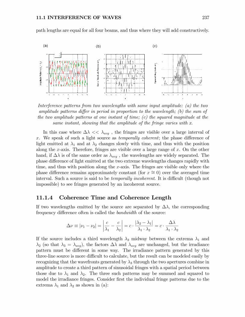
11.1 INTERFERENCE OF WAVES 237
path lengths are equal for all four beams, and thus where they will add constructively.
Interference patterns from two wavelengths with same input amplitude: (a) the twoamplitude patterns differ in period in proportion to the wavelength; (b) the sum ofthe two amplitude patterns at one instant of time; (c) the squared magnitude at the
same instant, showing that the amplitude of the fringe varies with x.
In this case where ∆λ << λavg , the fringes are visible over a large interval ofx. We speak of such a light source as temporally coherent ; the phase difference oflight emitted at λ1 and at λ2 changes slowly with time, and thus with the positionalong the x-axis. Therefore, fringes are visible over a large range of x. On the otherhand, if ∆λ is of the same order as λavg , the wavelengths are widely separated. Thephase difference of light emitted at the two extreme wavelengths changes rapidly withtime, and thus with position along the x-axis. The fringes are visible only where thephase difference remains approximately constant (for x ∼= 0) over the averaged timeinterval. Such a source is said to be temporally incoherent. It is difficult (though notimpossible) to see fringes generated by an incoherent source.
11.1.4 Coherence Time and Coherence Length
If two wavelengths emitted by the source are separated by ∆λ, the correspondingfrequency difference often is called the bandwidth of the source:
∆ν ≡ |ν1 − ν2| =¯c
λ1− c
λ2
¯= c · |λ2 − λ1|
λ1 · λ2= c · ∆λ
λ1 · λ2
If the source includes a third wavelength λ3 midway between the extrema λ1 andλ2 (so that λ3 = λavg), the factors ∆λ and λavg are unchanged, but the irradiancepattern must be different in some way. The irradiance pattern generated by thisthree-line source is more difficult to calculate, but the result can be modeled easily byrecognizing that the wavefronts generated by λ3 through the two apertures combine inamplitude to create a third pattern of sinusoidal fringes with a spatial period betweenthose due to λ1 and λ2. The three such patterns may be summed and squared tomodel the irradiance fringes. Consider first the individual fringe patterns due to theextrema λ1 and λ2 as shown in (a):
238 CHAPTER 11 WAVES AND IMAGING
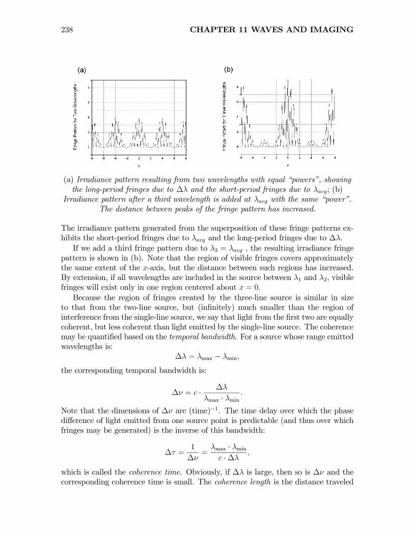
(a) Irradiance pattern resulting from two wavelengths with equal “powers”, showingthe long-period fringes due to ∆λ and the short-period fringes due to λavg; (b)
Irradiance pattern after a third wavelength is added at λavg with the same “power”.The distance between peaks of the fringe pattern has increased.
The irradiance pattern generated from the superposition of these fringe patterns ex-hibits the short-period fringes due to λavg and the long-period fringes due to ∆λ.If we add a third fringe pattern due to λ3 = λavg , the resulting irradiance fringe
pattern is shown in (b). Note that the region of visible fringes covers approximatelythe same extent of the x-axis, but the distance between such regions has increased.By extension, if all wavelengths are included in the source between λ1 and λ2, visiblefringes will exist only in one region centered about x = 0.Because the region of fringes created by the three-line source is similar in size
to that from the two-line source, but (infinitely) much smaller than the region ofinterference from the single-line source, we say that light from the first two are equallycoherent, but less coherent than light emitted by the single-line source. The coherencemay be quantified based on the temporal bandwidth. For a source whose range emittedwavelengths is:
∆λ = λmax − λmin,
the corresponding temporal bandwidth is:
∆ν = c · ∆λ
λmax · λmin.
Note that the dimensions of ∆ν are (time)−1. The time delay over which the phasedifference of light emitted from one source point is predictable (and thus over whichfringes may be generated) is the inverse of this bandwidth:
∆τ =1
∆ν=
λmax · λminc ·∆λ
,
which is called the coherence time. Obviously, if ∆λ is large, then so is ∆ν and thecorresponding coherence time is small. The coherence length is the distance traveled
11.1 INTERFERENCE OF WAVES 239
by an electromagnetic wave during the coherence time:
c ·∆τ ≡ ∆ =c
∆ν=
λmax · λmin∆λ
and is a measure of the length of the electromagnetic wave packet over which thephase difference is predictable. Recall that for interference of waves from a sourcewith wavelength range ∆λ, the range of coordinate x over which fringes are visible ishalf the period Dmod :
Dmod
2≡ 1
2 · sin [θ]
¯1
λ1− 1
λ2
¯−1=
1
2 · sin [θ]λmax · λmin
∆λ=
1
2 · sin [θ]
µ1
c ·∆ν
¶=
1
2 · sin [θ] ·∆
Thus the range of x over which fringes are visible is proportional to the coherencelength.
Lasers are the best available coherent sources; to a very good approximation,most lasers emit a single wavelength λ0 so that ∆λ = 0. The period of the mod-ulating sinusoid Dmod = ∞; fringes are visible at all x. A coherent source shouldbe employed when an optical interference pattern is used to measure a parameter ofthe system, such as the optical image quality (as was used to test the Hubble spacetelescope). Thus the range of x over which fringes are visible is determined by thecoherence length (and thus the bandwidth) of the source. Therefore, the visibility ofthe interference fringes may be used as a measure the source coherence.
11.1.5 Effect of Polarization of Electric Field on Fringe Vis-ibility
Up to this point, we have ignored the effect on the orientation of the electric fieldvectors on the sum of the fields. In fact, this is an essential consideration; twoorthogonal electric field vectors cannot add to generate a time-invariant modulationin the irradiance. Consider the sum of two electric field vectors E1 and E2 to generatea field E. The resulting irradiance is:
I = E •E = |E|2 = |E1 +E2|2
= (E1 +E2) · (E1 +E2)= (E1 •E1) + (E2 •E2) + (E1 •E2) + (E2 •E1)= (E1 •E1) + (E2 •E2) + 2(E1 •E2)= I1 + I2 + 2(E1 ·E2)
where I1 and I2 are the irradiances due to E1 and E2, respectively.
Consider the irradiance in the case where the incident fields are plane waves trav-
240 CHAPTER 11 WAVES AND IMAGING
eling in directions e1 and e2, respectively:
E1 = e1E1 cos [k1 • r− ω1t]
E2 = e2E2 cos [k2 • r− ω2t]
I = I1 + I2 + 2 he1E1 cos [k1 • r− ω1t] · e2E2 cos [k2 • r− ω2t]i= I1 + I2 + 2E1E2(e1 • e2) hcos [k1 • r− ω1t] cos [k2 • r− ω2t]i= I1 + I2 + 2E1E2(e1 • e2) hcos [(k1 − k2) • r− (ω1 − ω2) t]i= I1 + I2 + 2E1E2(e1 • e2) hcos [2kmod • r− 2ωmodt]i
In the case where the two components are polarized orthogonally so that e1 • e2 = 0,then the irradiance is the sum of the component irradiances and no interference isseen.In the case where ω1 = ω2 so that ωmod = 0, and I1 = I2, then the output
irradiance is:I = 2I1 (1 + cos [2kmod • r])
which again says that the irradiance includes a stationary sinusoidal fringe patternwith spatial period λmod =
2π|kmod|
.
11.2 Interferometers
We have seen several times now that optical interference results when two (or more)waves are superposed in such a way to produce a time-stationary spatial modulationof the superposed electric field, which may be observed by eye or a photosensitivedetector. Interferometers use this result to measure different parameters of the light(e.g., wavelength λ, bandwidth∆λ or coherence length∆ , angle and sphericity of thewavefront, etc.), or of the system (path length, traveling distance, index of refraction,etc.). Interferometers are generally divided into two classes that specify the method ofseparating a single wavefront into two (or more) wavefronts that may be recombined.The classes are division of wavefront and division of amplitude. The formertype has been considered; it divides wavefronts emitted by the source into two piecesand redirects one or both of them down different paths. They are recombined ina fashion such that k1 6= k2, even though |k1| = |k2|. The interference pattern isgenerated from the kmod portion of the sum of the wavefronts. Division-of-amplitudeinterferometers use a partially reflecting mirror — the beamsplitter — to divide thewavefront into two beams which travel down different paths and are recombined bythe original or another beamsplitter. The optical interference is generated by thephase difference between the recombined wavefronts.
11.2.1 Division-of-Amplitude Interferometers
This class of amplifiers are distinguished from the just-considered division-of-wavefrontinterferometers by the presence of a beamsplitter, which divides the incident radiation
11.2 INTERFEROMETERS 241
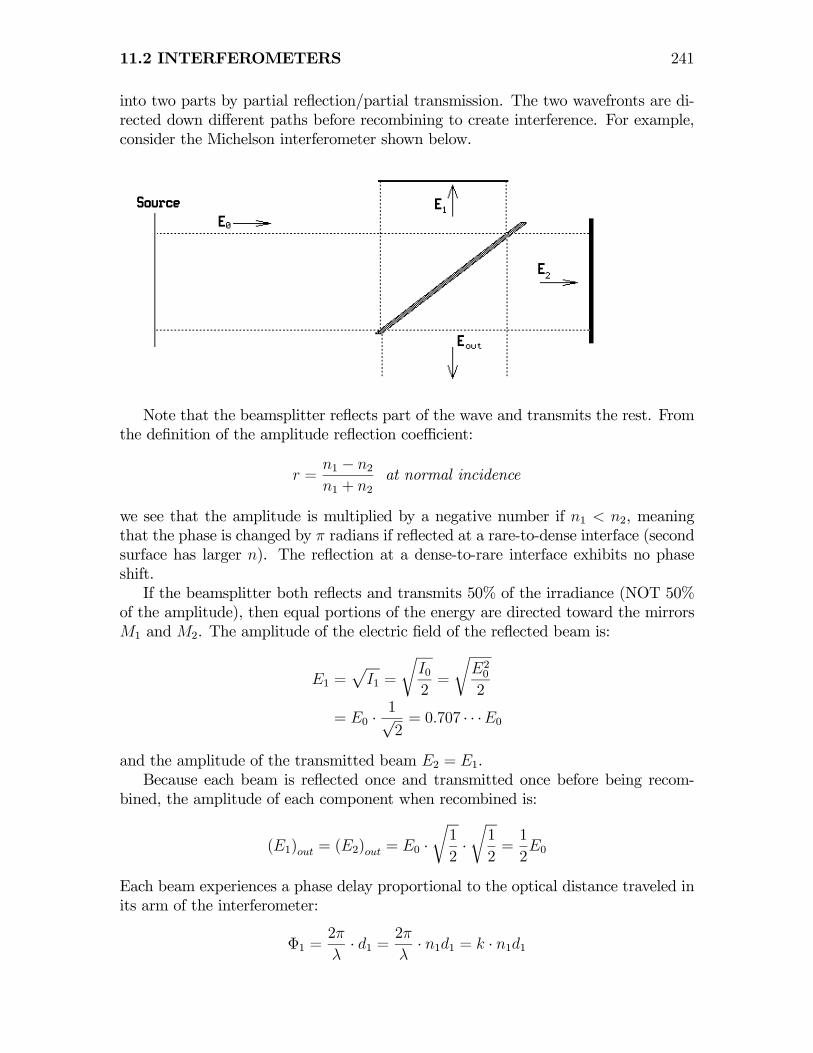
into two parts by partial reflection/partial transmission. The two wavefronts are di-rected down different paths before recombining to create interference. For example,consider the Michelson interferometer shown below.
Note that the beamsplitter reflects part of the wave and transmits the rest. Fromthe definition of the amplitude reflection coefficient:
r =n1 − n2n1 + n2
at normal incidence
we see that the amplitude is multiplied by a negative number if n1 < n2, meaningthat the phase is changed by π radians if reflected at a rare-to-dense interface (secondsurface has larger n). The reflection at a dense-to-rare interface exhibits no phaseshift.If the beamsplitter both reflects and transmits 50% of the irradiance (NOT 50%
of the amplitude), then equal portions of the energy are directed toward the mirrorsM1 and M2. The amplitude of the electric field of the reflected beam is:
E1 =pI1 =
rI02=
rE20
2
= E0 ·1√2= 0.707 · · ·E0
and the amplitude of the transmitted beam E2 = E1.Because each beam is reflected once and transmitted once before being recom-
bined, the amplitude of each component when recombined is:
(E1)out = (E2)out = E0 ·r1
2·r1
2=1
2E0
Each beam experiences a phase delay proportional to the optical distance traveled inits arm of the interferometer:
Φ1 =2π
λ· d1 =
2π
λ· n1d1 = k · n1d1

242 CHAPTER 11 WAVES AND IMAGING
where d1 is the distance traveled by beam #1 and n1 is the refractive index in thatpath (n = 1 in vacuum or air). The beam directed at mirror M1 travels distance L1from the beamsplitter to the mirror and again on the return, so the total physicalpath length d1 = 2L1. Similarly the physical length of the second path is d2 = 2L2and the optical path is n2d2 = 2n2L2. After recombination, the relative phase delayis:
∆Φ = Φ1 − Φ2 = k (n1d1 − n2d2)
= 2k (n1L1 − n2L2)
=4π
λ(n1L1 − n2L2)
Note that the phase delay is proporational to 1λ, i.e., longer wavelengths (red light)
experience smaller phase delays than shorter wavelengths (blue light).The amplitude at the detector is the sum of the amplitudes:
E(t) =E02cos
∙2π
λ· n1 · 2L1 − ω1t
¸+
E02cos
∙2π
λ· n2 · 2L2 − ω1t
¸=
E02
µcos
∙2π
λ· n1 · 2L1 − ω1t
¸+ cos
∙2π
λ· n2 · 2L2 − ω1t
¸¶which has the form cos [A] + cos [B], and thus may be rewritten as:
E(t) =2E02cos
∙2π (2n1L1 + 2n2L2)
2λ− 2πνt
¸· cos
∙2π (2n1L1 − 2n2L2)
2λ
¸= E0 cos
∙2π (n1L1 + n2L2)
λ− 2πνt
¸· cos
∙2π (n1L1 − n2L2)
λ
¸If the indices of refraction in the two paths are equal (usually n1 = n2 ∼= 1), then
the expression is simplified:
E(t) = E0 cos
∙2πn (L1 + L2)
λ− 2πνt
¸· cos
∙2πn (L1 − L2)
λ
¸= E0 cos
∙2π (L1 + L2)
λ− 2πνt
¸· cos
∙2π (L1 − L2)
λ
¸for n = 1
One of the multiplicative terms is a rapidly oscillating function of time; the other termis stationary in time. The time average of the squared magnitude is the irradiance:
I =|E(t)|2
®= E2
0
¿cos2
∙2π (L1 + L2)
λ− 2πνt
¸· cos2
∙2π (L1 − L2)
λ
¸À= E2
0
¿cos2
∙2π (L1 + L2)
λ− 2πνt
¸À· cos2
∙2π (L1 − L2)
λ
¸= E2
0 ·1
2cos
2∙2π (L1 − L2)
λ
¸

11.2 INTERFEROMETERS 243
The identity cos2 [θ] = 12(1 + cos [2θ]) may be used to recast the expression:
I = E20
1
2· 12
µ1 + cos
∙2π
λ· 2 (L1 − L2)
¸¶=
E20
4
µ1 + cos
∙2π
λ· 2 (L1 − L2)
¸¶Note that this is not a function of time or position, but only of the lenths of the armsof the interferometer and of λ. The Michelson interferometer with monochromaticplane-wave inputs generates a uniform irradiance related to the path difference. Ifinput wavefronts with other shapes are used, then fringes are generated whose periodis a function of the local optical path difference, which is directly related to the shapeof the wavefronts. If the incident light is a tilted plane wave, then the resultingpattern is analogous to that from a division-of-wavefront interferometer (Young’s
double-slit). If a point source emitting spherical waves is used, then the interfer-ometer may be modeled as:
Images of the point source are formed at S1 (due to mirror M1) and at S2 (due toM2). The wavefronts superpose and form interference fringes. The positions of thefringes may be determined from the optical path difference (OPD).

244 CHAPTER 11 WAVES AND IMAGING
The OPD is the excess distance that one wavefront has to travel relative to the otherbefore being recombined. For a ray oriented at angle θ measured relative to the axisof symmetry, the ray reflected from mirror M2 travels an extra distance:
OPD = 2 (L1 − L2) · cos [θ]
The symmetry about the central axis ensures that the fringes are circular. The phasedifference of the waves is the extra number of radians of phase that the wave musttravel in that OPD:
∆Φ = k ·OPD =2π
λ· 2 [L1 − L2] · cos [θ]
=4π · (L1 − L2) cos [θ]
λ[radians]
If the phase difference is a multiple of 2π radians, then the waves recombine inphase and a maximum of the amplitude results. If the phase difference is an oddmultiple of π radians, then the waves recombine out of phase and a minimum ofthe irradiance results due to destructive interference. The locations of constructiveinterference (irradiance maxima) may be specified by:
∆Φ = 2πm =4π · (L1 − L2) cos [θ]
λ→ mλ = 2 (L1 − L2) cos [θ]
The corresponding angles θ are specified by:
θ = cos−1∙
mλ
2 · (L1 − L2)
¸As the physical path difference L1 − L2 decreases, then mλ
2(L1−L2) increases and θdecreases. In other words, if the physical path difference is decreased, the angular sizeof a circular fringe decreases and the fringes disappear into the center of the pattern.Since a particular fringe occurs at the same angle relative to the optical axis, these

11.2 INTERFEROMETERS 245
are called fringes of equal inclination.If one mirror is tilted relative to the other, then the output beams travel in dif-
ferent directions when recombined. The fringes thus obtained are straight and havea constant spacing just like those from a Young’s double-slit experiment.
11.2.2 Applications of the Michelson Interferometer
1. Measure refractive index n: Insert a plane-parallel plate of known thickness tand unknown index n into one arm of a Michelson interferometer illuminatedwith light of wavelength λ. Count the number of fringes due to the plate:
OPD = (n− 1) t = ∆m · λ
2. Measure the wavelength of an unknown source or ∆λ between two spectral linesof a single source. Count the number of fringes that pass a single point as onemirror is moved a known distance.
3. Measure lengths of objects: The standard m now is defined in terms of a par-ticular spectral line:
1m = 1, 650, 763.73 wavelengths of emission at λ = 605.8 nm
from Kr-86 measured in vacuum
This standard has the advantage of being transportable.
4. Measure deflections of objects: The optical phase difference will be significantfor very small physical path differences. Place one mirror on an object andcount fringes to measure the deflection.
5. Measure the velocity of light (Michelson-Morley experiment)
11.2.3 Other Types of Division-of-Amplitude Interferome-ters
(2) Mach-Zehnder
The M-Z interferometer is very similar to the Michelson, except that a second beam-splitter is used to recombine the beams so that the light does not traverse the samepath twice. Therefore there is no factor of 2 in the OPD for the M-Z. Mach-Zehnderinterferometers often are used to measure the refractive index of liquids or gases. Thecontainer C1 (or C2) is filled with a gas while examining the fringe pattern. As thecontainer fills, the refractive index n increases and so does the optical path length inthat arm. The optical path difference is:
OPD = (n− 1) · δ
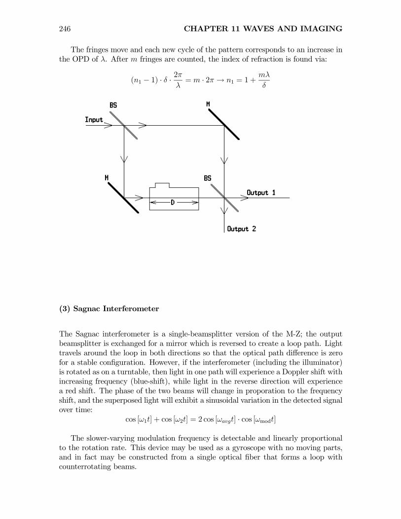
246 CHAPTER 11 WAVES AND IMAGING
The fringes move and each new cycle of the pattern corresponds to an increase inthe OPD of λ. After m fringes are counted, the index of refraction is found via:
(n1 − 1) · δ ·2π
λ= m · 2π → n1 = 1 +
mλ
δ
(3) Sagnac Interferometer
The Sagnac interferometer is a single-beamsplitter version of the M-Z; the outputbeamsplitter is exchanged for a mirror which is reversed to create a loop path. Lighttravels around the loop in both directions so that the optical path difference is zerofor a stable configuration. However, if the interferometer (including the illuminator)is rotated as on a turntable, then light in one path will experience a Doppler shift withincreasing frequency (blue-shift), while light in the reverse direction will experiencea red shift. The phase of the two beams will change in proporation to the frequencyshift, and the superposed light will exhibit a sinusoidal variation in the detected signalover time:
cos [ω1t] + cos [ω2t] = 2 cos [ωavgt] · cos [ωmodt]
The slower-varying modulation frequency is detectable and linearly proportionalto the rotation rate. This device may be used as a gyroscope with no moving parts,and in fact may be constructed from a single optical fiber that forms a loop withcounterrotating beams.
11.2 INTERFEROMETERS 247
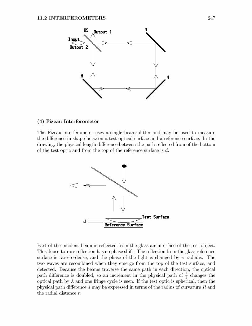
(4) Fizeau Interferometer
The Fizeau interferometer uses a single beamsplitter and may be used to measurethe difference in shape between a test optical surface and a reference surface. In thedrawing, the physical length difference between the path reflected from of the bottomof the test optic and from the top of the reference surface is d.
Part of the incident beam is reflected from the glass-air interface of the test object.This dense-to-rare reflection has no phase shift. The reflection from the glass referencesurface is rare-to-dense, and the phase of the light is changed by π radians. Thetwo waves are recombined when they emerge from the top of the test surface, anddetected. Because the beams traverse the same path in each direction, the opticalpath difference is doubled, so an increment in the physical path of λ
2changes the
optical path by λ and one fringe cycle is seen. If the test optic is spherical, then thephysical path difference d may be expressed in terms of the radius of curvature R andthe radial distance r:

248 CHAPTER 11 WAVES AND IMAGING
Pythagoras says that:
R2 = (R− d)2 + r2 =⇒ r2 = 2Rd− d2 ∼= 2Rd for d << R
d ∼= r2
2Rfor d << R
If the interstice between the optical elements in filled with air, and if m fringes arecounted between two points at radial distances r1 and r2, then the correspondingthickness change is:
m · λ2= OPD = nd→ d = m · λ
2in air
11.3 Diffraction
In geometrical (ray) optics, light is assumed to propagate in straight lines from thesource (rectilinear propagation). However, Grimaldi observed in the 1600s that thismodel does not conform to reality after light interacts with an obstruction. Grimaldiobserved that light deviates from straight-line propagation into the shadow region.He named this phenomenon diffraction. This spreading of a bundle of rays affects thesharpness of shadows cast by opaque objects; the edges become fuzzy because lightpropagates into the geometrical shadow region.

11.3 DIFFRACTION 249
Diffraction really is the same phenomenon as interference. In both, the wave characterof light creates stationary regions of constructive and destructive interference thatmay be observed as bright and dark regions. In the simplest case of two sources ofinfinitesmal size, the superposition wave may be determined by summing sphericalwave contributions from the sources; the effect is considered to be interference. Ifthe apertures are large (compared to the wavelength λ), then the spherical-wavecontributions from a large number of subsources are summed (by integrating overthe area of the aperture) to determine the total electric field. The superpositionelectric field vector (magnitude and phase) is the vector sum of the fields due to thesespherical-wave subsources. The mathematical model for diffraction is straightforwardto develop, though computations may be tedious.
Recall the form of a spherical wave emitted by a source located at the originof coordinates; energy conservation requires that the energy density of the electricfield of a spherical wave decrease as the square of the distance from the source.Correspondingly, the electric field decreases as the distance fom the source. Theelectric field observed at location [x1, y1, z1] due to a spherical wave emitted from theorigin is:
s [x1, y1, z1, t] =E0p
x21 + y21 + z21cos [kx · x+ ky · y + kz · z − ωt]
This observation that light from a point source generates a spherical wave is the firststep towards Huygen’s principle, which states that every point on a wavefront maybe modeled as a “secondary source” of spherical waves. The summation of the wavesfrom the secondary sources (sometimes called “wavelets”) produces a new wavefrontthat is “farther downstream” in the optical path.
250 CHAPTER 11 WAVES AND IMAGING
In the more general case of a spherical wave emitted from a source located atcoordinates [x0, y0, z0] and observed at [x1, y1, z1] has the form:
s [r, t] =E0|r| cos [k0•r− ω0t]→
E0|r| exp [k0•r− ω0t]
where |r| =p(x1 − x0)2 + (y1 − y0)2 + (z1 − z0)2 and |k0| = 2π
λ0.
For large |r|, the spherical wave may be approximated accurately as a paraboloidalwave, and for VERY large |r| the sphere becomes a plane wave. The region where thefirst approximation is acceptable defines Fresnel diffraction, while the more distantregion where the second approximation is valid is the Fraunhofer diffraction region.
11.3.1 Diffraction Integrals
Consider the electric field emitted from a point source located at [x0, y0, z0 = 0].The wave propagates in all directions. The electric field of that wave is observed onan observation plane centered about coordinate z1. The location in the observationplane is described by the two coordinates [x1, y1]. The electric field at [x1.y1] at thisdistance z1 from a source located in the plane [x0, y0] centered about z = z0 = 0 is:
E [x1, y1; z1, x0, y0, 0] =E0|r| cos [k0•r− ω0t] ,where |r| =
q(x1 − x0)2 + (y1 − y0)2 + z21
Though this may LOOK complicated, it is just an expression of the electric fieldpropagated as a spherical wave from a source in one plane to the observation pointin another plane; the amplitude decreases as the reciprocal of the distance and thephase is proportional to the distance and time. Diffraction calculations based on thesuperposition of spherical waves is Rayleigh-Sommerfeld diffraction.
Now, observe the electric field at that same location [x1, y1, z1] that is generatedfrom many point sources located in the x−y plane located at z = 0. The summationof the fields is computed as an integral of the electric fields due to each point source.The integral is over the area of the source plane. If all sources emit the same amplitudeE0, then the integral is simplified somewhat:
Etotal[x1, y1; z1] =
ZZ +∞
−∞E[x1, y1; z1;x0, y0, 0] dx0 dy0
=
ZZaperture
E0p(x1 − x0)2 + (y1 − y0)2 + z21
× cos∙2π
λ0·q(x1 − x0)2 + (y1 − y0)2 + z21 − ωt
¸dx0 dy0
This integral may be recast into a different form by defining the shape of the aperture

11.3 DIFFRACTION 251
to be a 2-D function f [x0, y0] in the source plane:
Etotal [x1, y1; z1]
= E0
ZZ +∞
−∞
f [x0, y0]p(x1 − x0)2 + (y1 − y0)2 + z21
× cos∙2π
λ0·q(x1 − x0)2 + (y1 − y0)2 + z21 − ωt
¸dx0dy0
This expression is the diffraction integral. Again, this expression LOOKS complicated,but really represents just the summation of the electric fields due to all point sources.Virtually the entire study of optical diffraction is the application of various schemes tosimplify and apply this equation. We will simplify it for two cases: (1) ObservationPlane z1 located near to the source plane z0 = 0; this is “near-field,” or “Fresneldiffraction” (the s in “Fresnel” is silent — the name is pronounced Fre 0·nel).(2) Observation Plane z1 located far enough from the source plane located z0 = 0
so that z1 ∼= ∞. This is called “far-field,” or “Fraunhofer diffraction,” which is par-ticularly interesting (and easier to compute results) because the diffraction integralis proportional to the Fourier transform of the object distribution (shape of the aper-ture).A schematic of the diffraction regions is shown in the figure.
Schematic of the diffraction regions for spherical waves emitted by a point source.Rayleigh-Sommerfeld diffraction is based on the spherical waves emitted by thesource. Fresnel diffraction is an approximation based on the assumption that the
252 CHAPTER 11 WAVES AND IMAGING
wavefronts are parabolic and with unit amplitude to ∞. The “width” of the quadraticphase is indicated by αn; this is the off-axis distance from the origin where the phasechange is π radians. Fraunhofer diffraction assumes that the spherical wave hastraveled a large distance and the wavefronts may be approximated by planes.
11.3.2 Fresnel Diffraction
Consider the first case of the diffraction integral where the observation plane is nearto the source plane, where the concept of near must be defined. Note that thedistance |r| appears twice in the expression for the electric field due to a point source— once in the denominator and once in the phase of the cosine. The first termaffects the size (magnitude) of the electric field, and the scalar product of the secondwith the wavevector k is computed to determine the rapidly changing phase angleof the sinusoid. Because the phase changes very quickly with time (because ω isvery large, ω ∼= 1015 radians/second) and with distance (because |k| is very small,|k| ∼= 10−7m), the phase difference of light observed at one point in the observationplane but generated from two points in the source plane may differ by MANY radians.Simply put, small changes in the propagation distance |r| have great significant tothe computation of the phase, but much less so when computing the amplitude ofthe electric field. Therefore, the distance may be approximated more crudely in thedenominator than in the phase.Now consider the approximation of the distance |r|. The complete expression is:
|r| =q(x1 − x0)2 + (y1 − y0)2 + z21
=
sz21 ·
µ1 +
(x1 − x0)2 + (y1 − y0)2
z21
¶
= z1 ·s1 +
(x1 − x0)2 + (y1 − y0)2
z21
= z1 ·µ1 +
(x1 − x0)2 + (y1 − y0)
2
z21
¶12
This is an EXACT expression that may be expanded into a power series by applyingthe binomial theorem. The general binomial expansion is:
(1 + α)n = 1+ nα+n · (n− 1)
2!α2 +
n · (n− 1) · (n− 2)3!
x3 + · · ·+ n!
(n− r)!r!αr + · · ·
This series converges to the correct value if α2 < 1. For the case n = 12(square root),
the result is:(1 + α)
12 = 1 +
α
2− 18α2 +
1
16α3 − · · ·
which leads to an expression for the distance |r|:
11.3 DIFFRACTION 253
|r| =q(x1 − x0)
2 + (y1 − y0)2 + z21 =
vuutz21
Ã1 +
(x1 − x0)2 + (y1 − y0)
2
z21
!
= z1
s1 +
(x1 − x0)2 + (y1 − y0)
2
z21
= z1
Ã1 +
1
2
(x1 − x0)2 + (y1 − y0)
2
z21− 18
¡(x1 − x0)
2 + (y1 − y0)2¢2
z41+ · · ·
!
If z1 is sufficiently large, terms of second and larger order may be assumed to besufficiently close to zero that they may be ignored, leaving the approximation:
|r| ∼= z1
Ã1 +
1
2
(x1 − x0)2 + (y1 − y0)
2
z21
!= z1 +
1
2
(x1 − x0)2 + (y1 − y0)
2
2z1
This may be simplified further by recasting the electric field expression into complexnotation:
E [x1, y1; z1, x0, y0, 0] ∼=E0z1Re
½exp
∙+2πi
λ
µz1 +
(x1 − x0)2 + (y1 − y0)
2
2z1
¶− 2πiνt
¸¾=
E0z1Re
½exp
∙+2πi
λz1
¸· exp [−2πiνt] · exp
∙+
iπ
λz1
¡(x1 − x0)
2 + (y1 − y0)2¢¸¾
The phase of this approximation of the spherical wave includes a constant phase 2πz1λ
, a time-varying phase −2πνt, and the last term whose phase is proportional to thesquare of the distance off-axis from the source point from the observation point. Inthe approximation, the wavefront emitted by a point source is not a sphere, but rathera paraboloid.
Note the unreasonable part of the assumption of Fresnel diffraction; the wavefrontis assumed to have constant squared magnitude regardless of the location [x1, y1]where the field is measured. In other words, the paraboloidal wave in Fresnel diffrac-tion has the same “brightness” regardless of how far off axis it is measured.
For larger values of z1 (observation plane farther from the source), the radius ofcurvature of the approximate paraboloidal waves increases, so the change in phasemeasured for nearby points in the observation plane decreases. As z1 approaches ∞,the paraboloid approaches a plane wave.
This electric field is substituted into the diffraction integral to obtain the approx-imate expression in the near-field:
254 CHAPTER 11 WAVES AND IMAGING
Etotal [x1, y1; z1] =
Z +∞
−∞E [x1, y1; z1;x0, y0, 0] dx0 dy0
∼= 1
z1exp
h³z1λ− νt
´iZZ +∞
−∞f [x0, y0] exp
∙iπ
λz1
¡(x1 − x0)
2 + (y1 − y0)2¢¸
dx0dy0
=1
z1exp
h³z1λ− νt
´i×ZZ +∞
−∞f [x0, y0] exp
∙iπ
λz1(x1 − x0)
2
¸exp
∙iπ
λz1(x1 − x0)
2
¸dx0 dy0
Again, this LOOKS complicated, but really is just a collection of the few parts thatwe have considered already. In words, the integral says that the electric field down-stream but near to the source function is the summation of paraboloidal fields fromthe individual sources. The paraboloidal approximation significantly simplifies thecomputation of the diffracted light.
11.3.3 Fresnel Diffraction Integral as a Convolution
Consider the Fresnel diffraction integral:
F [x1, y1] =
ZZ +∞
−∞f [x0, y0] exp
∙+
iπ
λz1
¡(x1 − x0)
2 + (y1 − y0)2¢¸ dx0dy0
Define the exponential to be a function h that depends on the four variables in aparticular way:
h [x1 − x0, y1 − y0] ≡ exp∙+
iπ
λz1
¡(x1 − x0)
2 + (y1 − y0)2¢¸
In other words, the Fresnel diffraction integral may be written as:
F [x1, y1] =
Z Z +∞
−∞f [x0, y0] h [x1 − x0, y1 − y0] dx0 dy0
Integral equations of this form abound in all areas of physical science, and particularlyin imaging; they are called convolution integrals. The function h is the shape of theintegral function and is often called the impulse response of the integral operator. Inimaging, and particularly in optics, the impulse response often is called the point-spread function. In other areas of physics, it has other names (e.g., Green’s function).The integral operator often is given a shorthand notation, such as the asterisk “∗.”The variables of integration also often are renamed as dummy variables, such as α,β:
F [x, y] =
Z Z +∞
−∞f [α, β] h [x− α, y − β] dα dβ
≡ f [x, y] ∗ h [x, y]
11.3 DIFFRACTION 255
where the form of the impulse response for Fresnel diffraction is:
h [x, y] =1
z1exp
h2πi
³z1λ− νt
´iexp
∙+i
π (x2 + y2)
λz1
¸This impulse response is called a “chirp” function — the real and imaginary parts areboth sinusoids with varying spatial frequency and that also differs with distance z1.The parameters of the chirp often are combined into
√λz1 ≡ α
h [x, y] =1
z1exp
h2πi
³z1λ− νt
´iexp
∙+iπ
x2 + y2
α2
¸so that the phase of the chirp function is π where
px2 + y2 = α. Again note that
the magnitude of the impulse response is the unit constant:
|h [x, y]| = 1 [x, y]
which indicates that the assumed illumination from a point source in the Fresneldiffraction region is constant off axis; there is no “inverse square law.” This obviouslyunphysical assumption limits the usefulness of calculated diffraction patterns to theimmediate vicinity of the optical axis of symmetry.
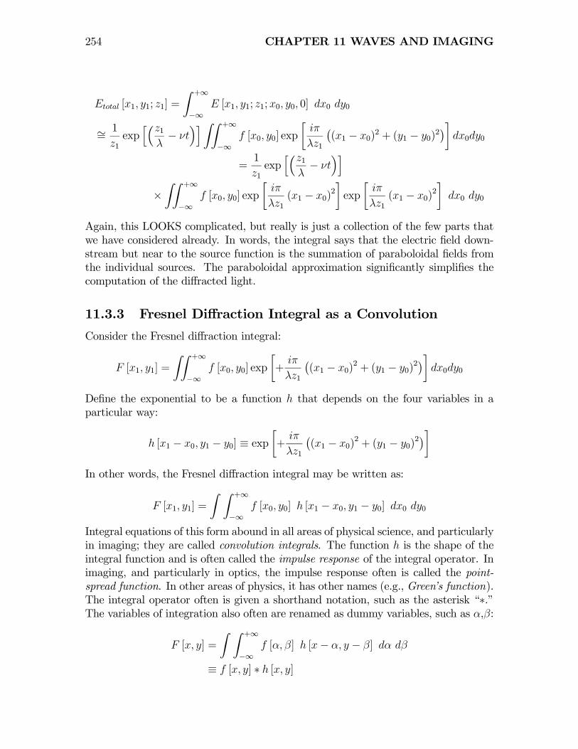
Profiles of the impulse response along a radial axis are shown for α = 1 and α = 2.The source distance is larger by a factor of four in the second case.

256 CHAPTER 11 WAVES AND IMAGING
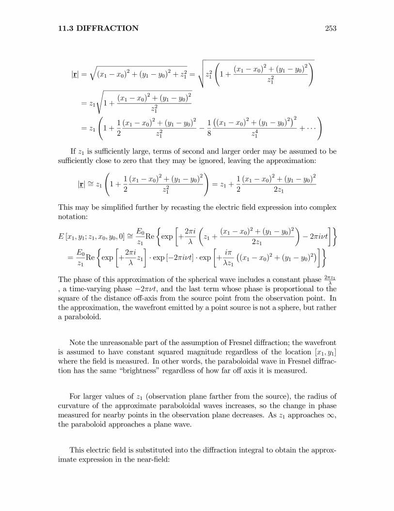
1-D profiles of the impulse response of Fresnel diffraction for (a)√λz1 = 1 and (b)√
λz1 = 2, so that z1 is four times larger in (b). Note that the phase increases lessrapidly with x for increasing distances from the source.
1-D profiles of the impulse response of Fresnel diffraction for λz1 = 1. Note that themagnitude of the impulse response is 1 and the phase is a quadratically increasingfunction of x.The convolution integral is straightforward to implement.
Computed Examples of Fresnel Diffraction
Below are computed simulations of the profiles of diffraction patterns that would begenerated from a knife edge at the same distances from the source as shown above.Note the “ringing” at the edges and that the fringes are farther apart when observedfarther from the source. Compare these images to actual Fresnel diffraction patterns
11.3 DIFFRACTION 257
in Hecht.
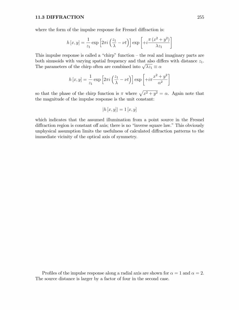
1-D profiles of the irradiance (squared magnitude) of diffraction patterns from asharp “knife edge” (modeled as the STEP function shown) for the same distancesfrom the origin: (a)
√λz1 = 1; (b)
√λz1 = 2 =⇒ z is four times larger. Note that
the “period” of the oscillation has increased with increasing distance from the sourceand that the irradiance at the origin is not zero but rather 1
4.
Since convolution is linear and shift invariant, the “images” of rectangular aperturesmay be calculated at these two distance by replicating the impulse responses, reversingone, and adding the amplitudes before computing the irradiance.
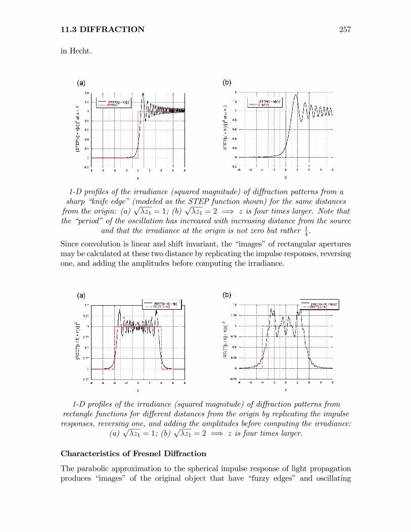
1-D profiles of the irradiance (squared magnitude) of diffraction patterns fromrectangle functions for different distances from the origin by replicating the impulseresponses, reversing one, and adding the amplitudes before computing the irradiance:
(a)√λz1 = 1; (b)
√λz1 = 2 =⇒ z is four times larger.
Characteristics of Fresnel Diffraction
The parabolic approximation to the spherical impulse response of light propagationproduces “images” of the original object that have “fuzzy edges” and oscillating

258 CHAPTER 11 WAVES AND IMAGING
Figure 11.2: The Fresnel diffraction patterns of at the same distance from the originfor two rectangles with different widths, showing that the “width” of the Fresnel patternis proportional to the width of the object.
amplitude on the bright side of an edge. At a fixed distance from the object, thewidth of the diffraction pattern is proportional to the width of the original object; ifthe object becomes wider, so does the “image” in the Fresnel diffraction pattern.
11.3.4 Diffraction Integral Valid Far from Source
The diffraction integral may be further simplified for the case where the distancefrom the source to the observation plane is sufficiently large to allow the electric fieldfrom an individual source to be approximated by a plane wave. The process may beconsidered for one of the paraboloidal waves:
exp
∙iπ
λz1
¡(x1 − x0)
2 + (y1 − y0)2¢¸
= exp
∙iπ(x20 + y20)
λz1
¸· exp
∙iπ(x21 + y21)
λz1
¸· exp
∙−i2πλz1
(x0x1 + y0y1)
¸If the source is restricted to be near to the optical axis so that x0, y0 ∼= 0 (or, morerigorously, if x20 + y20 << λz1), then
(x20 + y20)
λz1∼= 0
and:
exp
∙iπ(x20 + y20)
λz1
¸∼= 1.
11.3 DIFFRACTION 259
Similarly, if the observation point is near to the optic axis so that x21 + y21 << λz1,then:
exp
∙iπ(x21 + y21)
λz1
¸∼= 1.
Though x0 and x1 are sufficiently small for these approximations, the third exponen-tial term is retained because their difference may be larger:
exp
∙iπ
λz1
¡(x1 − x0)
2 + (y1 − y0)2¢¸ ∼= exp ∙−2πi (x0x1 + y0y1)
λz1
¸Considered in the observation plane as functions of x1 and y1, the phase of the wave-front is proportional to the source variables [x0, y0]; the wavefront is a plane. Thecorresponding approximation for the diffraction integral is:
Etotal [x1, y1; z1] =1
z1exp
h2πi
³z1λ− νt
´i·ZZ +∞
−∞f [x0, y0] exp
∙−2πi (x0x1 + y0y1)
λz1
¸dx0 dy0
The diffracted light far from the source is a summation of the plane waves generated byeach source point. This is called the Fraunhofer diffraction formula, and the resultingpatterns are VERY different from Fresnel diffraction from the same aperture. In fact,the formula can be interpreted as a Fourier transform where the frequency coordinatesare mapped back to the space domain via ξ = x1
λz1, η = y1
λz1:
Etotal [x1, y1; z1] =
µ1
z1exp
h2πi
³z1λ− νt
´i¶·ZZ +∞
−∞f [x0, y0] exp
∙−2πi
µx0
∙x1λz1
¸+ y0
∙y1λz1
¸¶¸dx0 dy0
=
µ1
z1exp
h2πi
³z1λ− νt
´i¶· F2 {f [x, y]}|ξ= x1
λz1,η=
y1λz1
The resulting irradiance patterns are the squared magnitudes of the fields. TheFourier transform relationship means that the diffraction patterns (the “images”)scale in inverse proportion to the original functions; larger input functions f [x, y]produce smaller (and brighter) diffraction patterns.
Computed Examples of Fraunhofer Diffraction
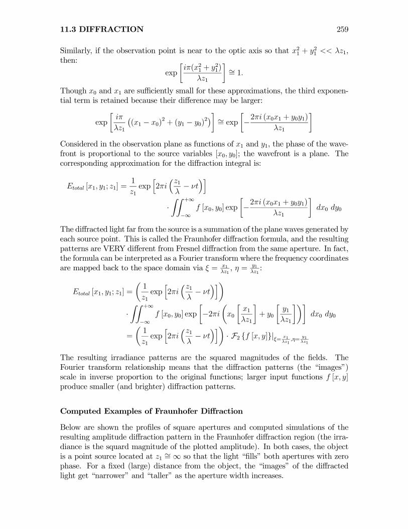
Below are shown the profiles of square apertures and computed simulations of theresulting amplitude diffraction pattern in the Fraunhofer diffraction region (the irra-diance is the squard magnitude of the plotted amplitude). In both cases, the objectis a point source located at z1 ∼=∞ so that the light “fills” both apertures with zerophase. For a fixed (large) distance from the object, the “images” of the diffractedlight get “narrower” and “taller” as the aperture width increases.

260 CHAPTER 11 WAVES AND IMAGING
1-D profiles of Fraunhofer diffraction patterns: (a) input objects are two rectanglesthat differ in width; (b) amplitude (NOT irradiance) of the correspondingFraunhofer diffraction patterns, showing that the wider aperture produces a
“brighter” and “narrower” amplitude distributions.
A useful measure of the “width” of the Fraunhofer pattern is labeled for both cases;this is the distance from the center of symmetry to the first zero. This “width” is ameasure of the ability of the system to resolve fine detail, because two point sourceswould each generate their own diffraction pattern. As the angular separation of thepoint sources decreases, it would be more difficult to distinguish that there are twooverlapping patterns.

11.3 DIFFRACTION 261
Illustrations of resolution in Fraunhofer diffraction: (a) individual images of twopoint sources in the Fraunhofer domain; (b) sum of the two images, showing thatthey may be distinguished easily; (c) images of two sources that are closer together;
(d) sum showing that it is much more difficult to distinguish the sources.
Fraunhofer Diffraction in Optical Imaging Systems
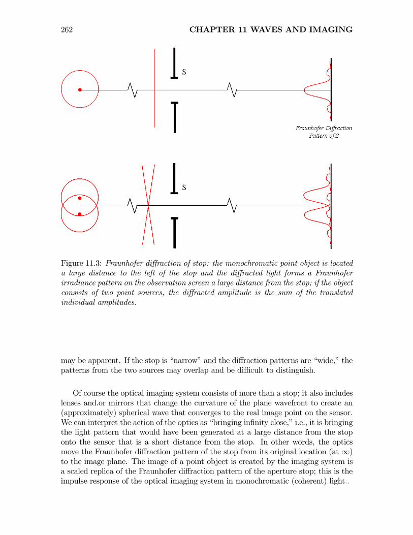
Consider a monochromatic point object located a long distance away from an imagingsystem, so that the wavefronts are approximately plane waves. The entrance pupil ofthe optical system (an image of the aperture stop) “selects” a portion of a plane wave.If the system consisted only of the entrance pupil (which would then be identical tothe aperture stop), then the light would continue to propagate. If observed a longdistance from the stop, we would see the Fraunhofer diffraction pattern of the stop;the smaller the stop, the larger the diffraction pattern. If the object consisted of twomonochromatic point sources displaced by a small angle, the diffracted amplitudewould be the sum of two replicas of the Fraunhofer diffracted amplitude slightlydisplaced. The observed irradiance is the time average of the squared magnitude ofthis amplitude. If the aperture stop is “wide” in some sense, then the diffractionpatterns will be “narrow” and the fact that the object consisted of two points sources
262 CHAPTER 11 WAVES AND IMAGING
Figure 11.3: Fraunhofer diffraction of stop: the monochromatic point object is locateda large distance to the left of the stop and the diffracted light forms a Fraunhoferirradiance pattern on the observation screen a large distance from the stop; if the objectconsists of two point sources, the diffracted amplitude is the sum of the translatedindividual amplitudes.
may be apparent. If the stop is “narrow” and the diffraction patterns are “wide,” thepatterns from the two sources may overlap and be difficult to distinguish.
Of course the optical imaging system consists of more than a stop; it also includeslenses and.or mirrors that change the curvature of the plane wavefront to create an(approximately) spherical wave that converges to the real image point on the sensor.We can interpret the action of the optics as “bringing infinity close,” i.e., it is bringingthe light pattern that would have been generated at a large distance from the stoponto the sensor that is a short distance from the stop. In other words, the opticsmove the Fraunhofer diffraction pattern of the stop from its original location (at ∞)to the image plane. The image of a point object is created by the imaging system isa scaled replica of the Fraunhofer diffraction pattern of the aperture stop; this is theimpulse response of the optical imaging system in monochromatic (coherent) light..

11.3 DIFFRACTION 263
An optical system imaging a point source creates a scaled replica the Fraunhoferdiffraction pattern of the stop on the image plane. In other words, the impulse
response of the imaging system is the Fraunhofer diffraction pattern of the aperturestop.
Effect of Diffraction on Image Quality
The spreading of light from rectilinear propagation that may be modeled as prop-agation of spherical waves that is called diffraction provides the fundamental andultimate limitation on the capability of an optical system to create images. Considerthe image of a point source located at an infinite distance from a simple single-lensimaging system. The source generates a spherical wave that is collected by the pupilof the lens. The lens tries to change the curvature to create a converging sphericalwave that forms perfect point image at the focal point of the lens. However, the prin-ciples of diffraction require that every point at the pupil of the lens is a point sourceof spherical waves that are summed to create the image. For this sum to create anideal point image, the electric fields from all points in the pupil would have to cancelexactly everywhere except at the ideal image point, which cannot happen. Instead,the electric fields superpose and the resulting irradiance creates an image whose sizeand shape depends on the size and shape of the pupil. In other words, diffraction oflight from the pupil of the lens determines the size of the image of the ideal pointsource.The optical elements in most imaging systems have circular cross-sections. The
diffraction pattern of the circular pupil also is circularly symmetric, but has a finitesize (linear extent). If two point sources are sufficiently close together (separatedby a small angle), the circularly symmetric images will overlap, and may not bedistinguishable. The smallest angular separation that produces separable imagesdetermines the resolution of the imaging system. Without proof, we present theequation derived by Lord Rayleight for the resolution of the imaging system. If thesources emit light at wavelength λ, are located a distance L from the lens, and areseparated by a distance d, the diameter D of the image spot is:
D ∝ Lλ
d

264 CHAPTER 11 WAVES AND IMAGING
Note the similarity to the formula for the separation between interference fringes inYoung’s experiment. The angular diameter of the image spot is:
∆θ ∼= d
L
which implies the relationship:
∆θ ∝ λ
D
The more accurate relation for imaging elements with circular cross-sections is:
∆θ ∼= 1.22 λD.
For the 200-diameter Hale telescope on Palomar Mountain, the theoretical min-imum angular separation is ∆θ ∼= 0.24λ, for λ measured in meters. In green light(λ = 550 nm), the angular separation is:
∆θ ∼= 1.32 · 10−7radians = 0.132 µradians ∼= 0.03 arc-seconds
Of course, the ultimate resolution of the Hale telescope actually is limited by at-mospheric turbulence, which creates random variations in the air temperature andthus in the refractive index. These variations are often decomposed into the aberra-tions introduced into the wavefront by the phase errors. The constant phase (“pis-ton”) error has no effect on the irradiance, the squared magnitude of the ampli-tude). Linear phase errors (“tip-tilt”) move the image from side to side and up-down.Quadratic phase errors (“defocus”) act like additional lenses that move the imageplane backwards or forwards along the optical axis. In general, the tip-tilt erroris the most significant, which means that correcting this aberration signficantly im-proves the image quality. The field of correcting atmospheric aberrations is called“adaptive optics,” and is an active research area.The diameter of the primary mirror of the Hubbell space telescope is approxi-
mately 1/2 that of the Hale telescope (D ∼= 2.4m), so the angular resolution of theoptics at 550nm is approximately twice as large (0.26µrad ∼= 0.6 arc-seconds). Ofcourse, there is no atmosphere to mess up the Hubble images.
Related Documents


