Chapter 11: Output and Expenditure in the Short Run © 2008 Prentice Hall Business Publishing Economics R. Glenn Hubbard, Anthony Patrick O’Brien, 2e. 1 of 54 Output and Expenditure in the Short Run Aggregate expenditure (AE) The total amount of spending on the economy’s output: Aggregate Expenditure • Consumption (C) • Planned Investment (I) • Government Purchases of Goods + Services (G) • Net Exports (NX) Actual investment in a year can differ from planned investment: businesses “invest” in unintended inventories if sales fall short of what they expected AE = C + I + G + NX Macroeconomic Equilibrium: Aggregate Expenditure = Output (Y) AE = C + I + G + NX = Y

Chapter 11: Output and Expenditure in the Short Run © 2008 Prentice Hall Business Publishing Economics R. Glenn Hubbard, Anthony Patrick O’Brien, 2e. 1.
Dec 18, 2015
Welcome message from author
This document is posted to help you gain knowledge. Please leave a comment to let me know what you think about it! Share it to your friends and learn new things together.
Transcript

Ch
apte
r 11
: O
utp
ut
and
Ex
pen
dit
ure
in
th
e S
ho
rt R
un
© 2008 Prentice Hall Business Publishing Economics R. Glenn Hubbard, Anthony Patrick O’Brien, 2e. 1 of 54
Output and Expenditure in the Short Run
Aggregate expenditure (AE) The total amount of spending on the economy’s output:
Aggregate Expenditure
• Consumption (C)
• Planned Investment (I)
• Government Purchases of Goods + Services (G)
• Net Exports (NX)
Actual investment in a year can differ from planned investment: businesses “invest” in unintended inventories if sales fall short of what they expected
AE = C + I + G + NX
Macroeconomic Equilibrium: Aggregate Expenditure = Output (Y)
AE = C + I + G + NX = Y

Ch
apte
r 11
: O
utp
ut
and
Ex
pen
dit
ure
in
th
e S
ho
rt R
un
© 2008 Prentice Hall Business Publishing Economics R. Glenn Hubbard, Anthony Patrick O’Brien, 2e. 2 of 54
EXPENDITURE CATEGORY
EXPENDITURE(BILLIONS OF 2000 DOLLARS)
Consumption $8,091
Investment 1,946
Government 1,998
Net Exports −618
Components of Real Aggregate Expenditure, 2006

Ch
apte
r 11
: O
utp
ut
and
Ex
pen
dit
ure
in
th
e S
ho
rt R
un
© 2008 Prentice Hall Business Publishing Economics R. Glenn Hubbard, Anthony Patrick O’Brien, 2e. 3 of 54
The Aggregate Expenditure ModelAdjustments to Macroeconomic Equilibrium
IF … THEN … AND …
Aggregate expenditure isequal to GDP
inventories areunchanged
the economy is inmacroeconomic equilibrium.
Aggregate expenditure isless than GDP inventories rise
GDP and employmentdecrease.
Aggregate Expenditure isgreater than GDP inventories fall
GDP and employmentincrease.
Actual investment in a year can differ from planned investment: businesses “invest” in unintended inventories if sales fall short of what they expected

Ch
apte
r 11
: O
utp
ut
and
Ex
pen
dit
ure
in
th
e S
ho
rt R
un
© 2008 Prentice Hall Business Publishing Economics R. Glenn Hubbard, Anthony Patrick O’Brien, 2e. 4 of 54
Real Consumption Expenditure C = $C/CPI
FIGURE 11-1
Real Consumption, 1979–2006
Ch
apte
r 11
: O
utp
ut
and
Ex
pen
dit
ure
in
th
e S
ho
rt R
un
© 2008 Prentice Hall Business Publishing Economics R. Glenn Hubbard, Anthony Patrick O’Brien, 2e. 5 of 54
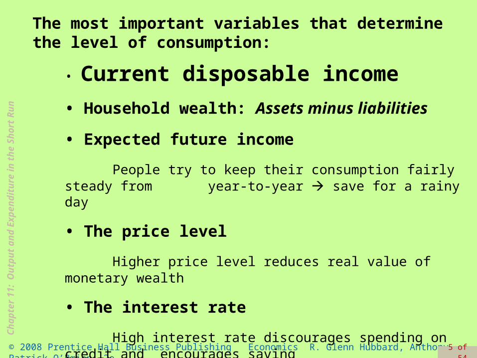
• Current disposable income
• Household wealth: Assets minus liabilities
• Expected future income
People try to keep their consumption fairly steady from year-to-year save for a rainy day
• The price level
Higher price level reduces real value of monetary wealth
• The interest rate
High interest rate discourages spending on credit and encourages saving
The most important variables that determine the level of consumption:
Ch
apte
r 11
: O
utp
ut
and
Ex
pen
dit
ure
in
th
e S
ho
rt R
un
© 2008 Prentice Hall Business Publishing Economics R. Glenn Hubbard, Anthony Patrick O’Brien, 2e. 6 of 54
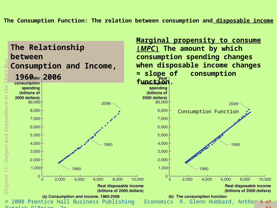
The Relationship between Consumption and Income,
1960– 2006
The Consumption Function: The relation between consumption and disposable income
Consumption Function
Marginal propensity to consume (MPC) The amount by which consumption spending changes when disposable income changes = slope of consumption function.

Ch
apte
r 11
: O
utp
ut
and
Ex
pen
dit
ure
in
th
e S
ho
rt R
un
© 2008 Prentice Hall Business Publishing Economics R. Glenn Hubbard, Anthony Patrick O’Brien, 2e. 7 of 54
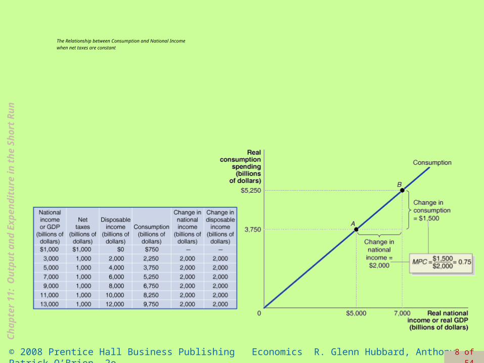
Marginal propensity to consume (MPC) The slope of the consumption function: The amount by which consumption spending changes when disposable income changes.
YD
CMPC
income disposablein Change
nconsumptioin Change
The Consumption Function
We can also use the MPC to determine how much consumption will change as income changes:
income disposablein Change
nconsumptioin ChangeMPC
Change in consumption = Change in disposable income × MPC
Ch
apte
r 11
: O
utp
ut
and
Ex
pen
dit
ure
in
th
e S
ho
rt R
un
© 2008 Prentice Hall Business Publishing Economics R. Glenn Hubbard, Anthony Patrick O’Brien, 2e. 8 of 54
The Relationship between Consumption and National Income
when net taxes are constant

Ch
apte
r 11
: O
utp
ut
and
Ex
pen
dit
ure
in
th
e S
ho
rt R
un
© 2008 Prentice Hall Business Publishing Economics R. Glenn Hubbard, Anthony Patrick O’Brien, 2e. 9 of 54
National income = Consumption + Saving + Taxes
Change in national income = Change in consumption + Change in saving + Change in taxes
Y = C + S + T
Determining the Level of Aggregate Expenditure in the Economy
Income, Consumption, and Saving
TSCY If taxes are always a constant amount, ΔT = 0
ΔΔY = Y = ΔΔC + C + ΔΔSS

Ch
apte
r 11
: O
utp
ut
and
Ex
pen
dit
ure
in
th
e S
ho
rt R
un
© 2008 Prentice Hall Business Publishing Economics R. Glenn Hubbard, Anthony Patrick O’Brien, 2e. 10 of 54
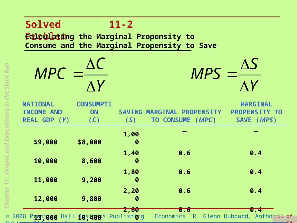
Marginal propensity to save (MPS) The change in saving divided by the change in disposable income.
Income, Consumption, and Saving
Y
S
Y
C
Y
Y
or,
1 = MPC + MPS
MPS = 1 - MPC
Ch
apte
r 11
: O
utp
ut
and
Ex
pen
dit
ure
in
th
e S
ho
rt R
un
© 2008 Prentice Hall Business Publishing Economics R. Glenn Hubbard, Anthony Patrick O’Brien, 2e. 11 of 54
Solved Problem 11-2Calculating the Marginal Propensity to Consume and the Marginal Propensity to Save
Y
CMPC
Y
SMPS
NATIONAL INCOME AND REAL GDP (Y)
CONSUMPTION(C)
SAVING(S)
MARGINAL PROPENSITY TO CONSUME (MPC)
MARGINAL PROPENSITY TO
SAVE (MPS)
$9,000 $8,000 1,000
— —
10,000 8,600 1,4000.6 0.4
11,000 9,200 1,8000.6 0.4
12,000 9,800 2,2000.6 0.4
13,000 10,400 2,6000.6 0.4
Ch
apte
r 11
: O
utp
ut
and
Ex
pen
dit
ure
in
th
e S
ho
rt R
un
© 2008 Prentice Hall Business Publishing Economics R. Glenn Hubbard, Anthony Patrick O’Brien, 2e. 12 of 54
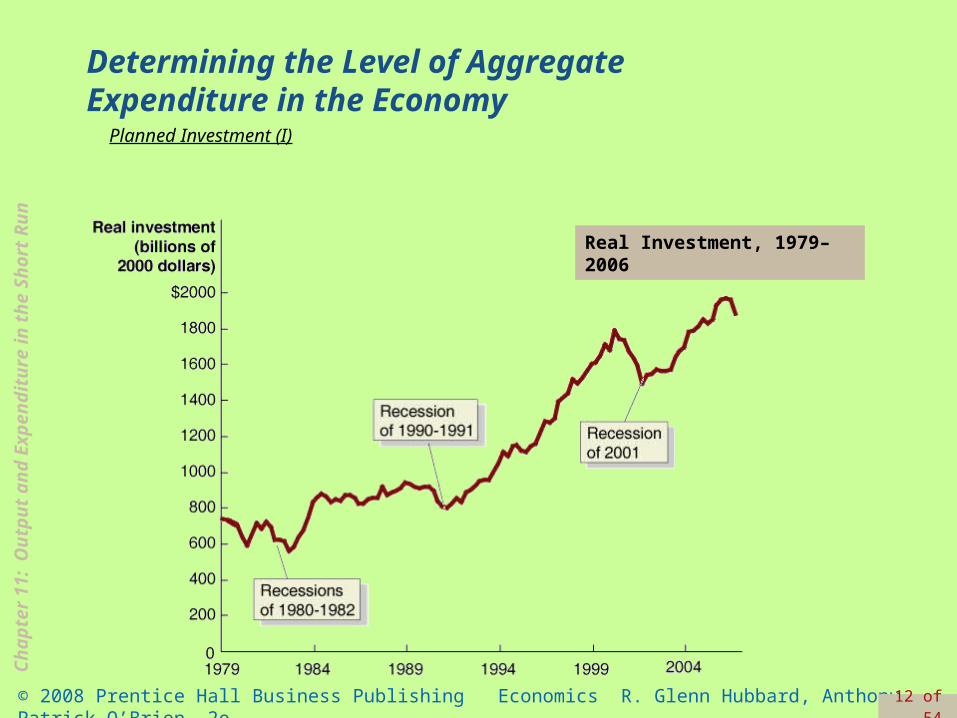
Real Investment, 1979–2006
Determining the Level of Aggregate Expenditure in the Economy
Planned Investment (I)

Ch
apte
r 11
: O
utp
ut
and
Ex
pen
dit
ure
in
th
e S
ho
rt R
un
© 2008 Prentice Hall Business Publishing Economics R. Glenn Hubbard, Anthony Patrick O’Brien, 2e. 13 of 54
• Expectations of future profitability
Waves of optimism and pessimism
• Major technology changes: new products & processes
• The interest rate
• Taxes
• Cash flow
• Current capacity utilization
The most important variables that determine the level of investment:

Ch
apte
r 11
: O
utp
ut
and
Ex
pen
dit
ure
in
th
e S
ho
rt R
un
© 2008 Prentice Hall Business Publishing Economics R. Glenn Hubbard, Anthony Patrick O’Brien, 2e. 14 of 54
The “new” information economy of the 1990s

Ch
apte
r 11
: O
utp
ut
and
Ex
pen
dit
ure
in
th
e S
ho
rt R
un
© 2008 Prentice Hall Business Publishing Economics R. Glenn Hubbard, Anthony Patrick O’Brien, 2e. 15 of 54
Real Government Purchases, 1979–2006
Government Purchases (G)

Ch
apte
r 11
: O
utp
ut
and
Ex
pen
dit
ure
in
th
e S
ho
rt R
un
© 2008 Prentice Hall Business Publishing Economics R. Glenn Hubbard, Anthony Patrick O’Brien, 2e. 16 of 54
Real Net Exports, 1979–2006
Net Exports (NX)

Ch
apte
r 11
: O
utp
ut
and
Ex
pen
dit
ure
in
th
e S
ho
rt R
un
© 2008 Prentice Hall Business Publishing Economics R. Glenn Hubbard, Anthony Patrick O’Brien, 2e. 17 of 54
• The price level in the United States relative to the price levels in other countries
• The growth rate of GDP in the United States relative to the growth rates of GDP in other countries
• The exchange rate between the dollar and other currencies
Net Exports (NX)
The most important variables that determine the level of net exports:
Ch
apte
r 11
: O
utp
ut
and
Ex
pen
dit
ure
in
th
e S
ho
rt R
un
© 2008 Prentice Hall Business Publishing Economics R. Glenn Hubbard, Anthony Patrick O’Brien, 2e. 18 of 54
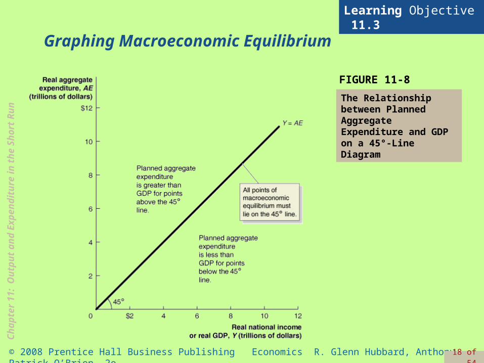
Learning Objective 11.3
FIGURE 11-8
The Relationship between Planned Aggregate Expenditure and GDP on a 45°-Line Diagram
Graphing Macroeconomic Equilibrium

Ch
apte
r 11
: O
utp
ut
and
Ex
pen
dit
ure
in
th
e S
ho
rt R
un
© 2008 Prentice Hall Business Publishing Economics R. Glenn Hubbard, Anthony Patrick O’Brien, 2e. 19 of 54
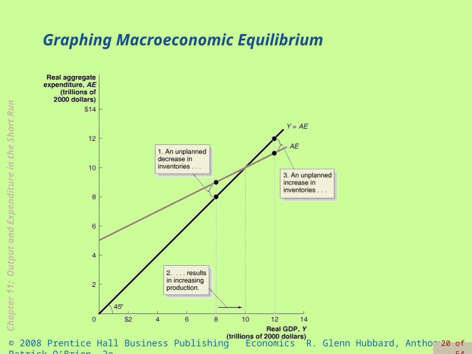
Graphing Macroeconomic Equilibrium
Ch
apte
r 11
: O
utp
ut
and
Ex
pen
dit
ure
in
th
e S
ho
rt R
un
© 2008 Prentice Hall Business Publishing Economics R. Glenn Hubbard, Anthony Patrick O’Brien, 2e. 20 of 54
Graphing Macroeconomic Equilibrium
Ch
apte
r 11
: O
utp
ut
and
Ex
pen
dit
ure
in
th
e S
ho
rt R
un
© 2008 Prentice Hall Business Publishing Economics R. Glenn Hubbard, Anthony Patrick O’Brien, 2e. 21 of 54
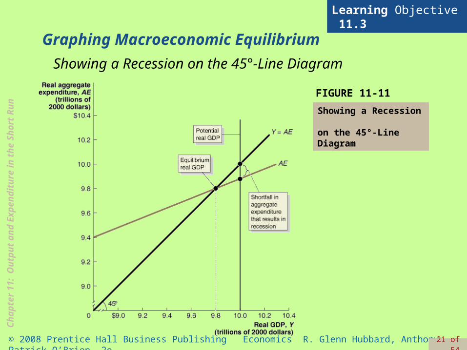
Graphing Macroeconomic Equilibrium
Learning Objective 11.3
FIGURE 11-11
Showing a Recession on the 45°-Line Diagram
Showing a Recession on the 45°-Line Diagram
Ch
apte
r 11
: O
utp
ut
and
Ex
pen
dit
ure
in
th
e S
ho
rt R
un
© 2008 Prentice Hall Business Publishing Economics R. Glenn Hubbard, Anthony Patrick O’Brien, 2e. 22 of 54
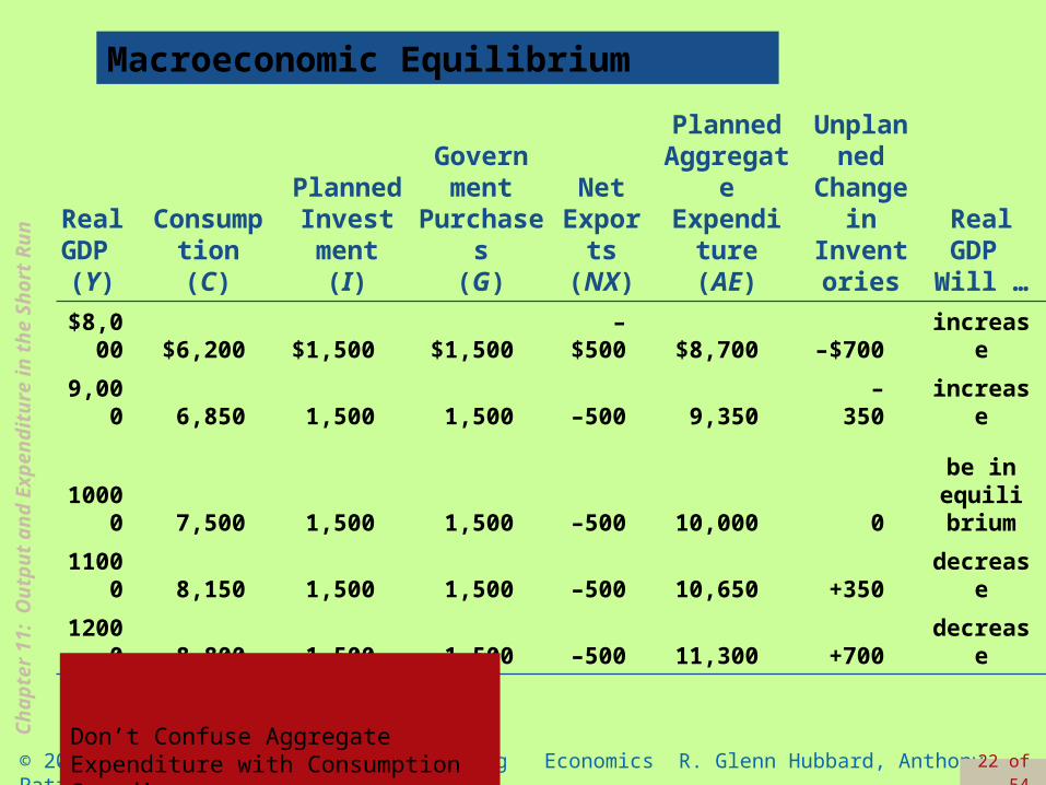
Real GDP
(Y)
Consump tion(C)
Planned Invest ment
(I)
Govern ment
Purchases
(G)
Net Export
s(NX)
Planned Aggregate Expendi
ture(AE)
Unplan ned
Change in Invent
ories
Real GDP
Will …
$8,000 $6,200 $1,500 $1,500
– $500 $8,700 –$700 increase
9,000 6,850 1,500 1,500 –500 9,350 –350 increase
10000 7,500 1,500 1,500 –500 10,000 0
be in equili brium
11000 8,150 1,500 1,500 –500 10,650 +350 decrease
12000 8,800 1,500 1,500 –500 11,300 +700 decrease
Don’t Let This Happen to YOU!Don’t Confuse Aggregate Expenditure with Consumption Spending
Macroeconomic Equilibrium
Ch
apte
r 11
: O
utp
ut
and
Ex
pen
dit
ure
in
th
e S
ho
rt R
un
© 2008 Prentice Hall Business Publishing Economics R. Glenn Hubbard, Anthony Patrick O’Brien, 2e. 23 of 54
The Multiplier Effect

Ch
apte
r 11
: O
utp
ut
and
Ex
pen
dit
ure
in
th
e S
ho
rt R
un
© 2008 Prentice Hall Business Publishing Economics R. Glenn Hubbard, Anthony Patrick O’Brien, 2e. 24 of 54
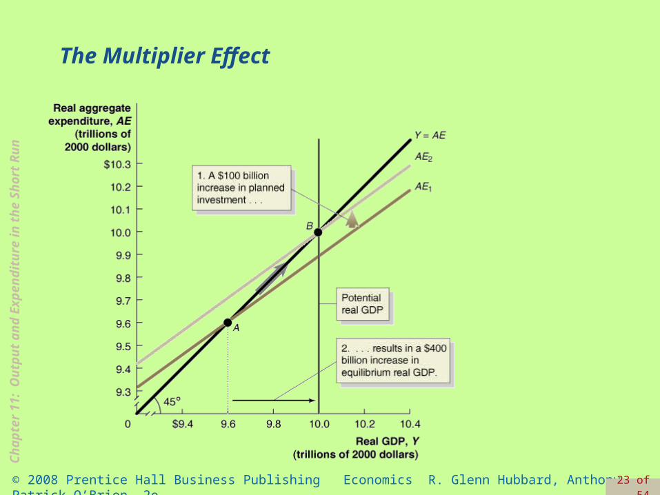
Learning Objective 11.4
The Multiplier Effect
Autonomous expenditure An expenditure that does not depend on the level of GDP.
Multiplier The increase in equilibrium real GDP in response to increase in autonomous expenditure, e.g.
Expenditure multiplier = ΔY/ΔI
Multiplier effect The process by which an increase in autonomous
expenditure leads to a larger increase in real GDP: ΔY = ΔI + ΔC
= Change in autonomous spending that sparks an expansion
+
Change in consumption spending induced by increasing output and income.
Ch
apte
r 11
: O
utp
ut
and
Ex
pen
dit
ure
in
th
e S
ho
rt R
un
© 2008 Prentice Hall Business Publishing Economics R. Glenn Hubbard, Anthony Patrick O’Brien, 2e. 25 of 54
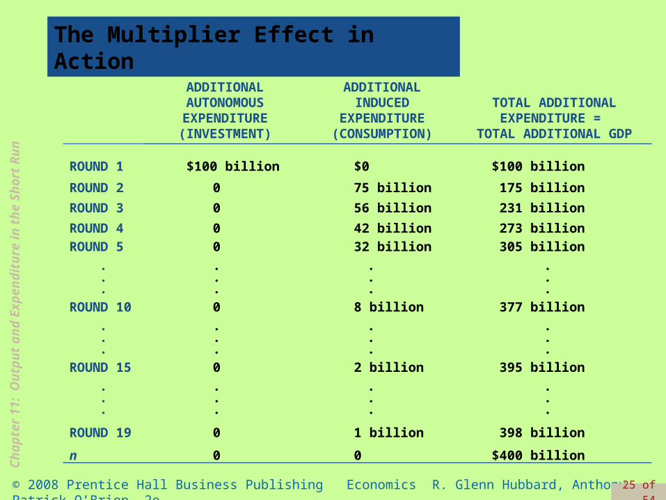
The Multiplier Effect in Action
ADDITIONAL AUTONOMOUS EXPENDITURE (INVESTMENT)
ADDITIONAL INDUCED
EXPENDITURE(CONSUMPTION)
TOTAL ADDITIONAL EXPENDITURE =
TOTAL ADDITIONAL GDP
ROUND 1 $100 billion $0 $100 billion
ROUND 2 0 75 billion 175 billion
ROUND 3 0 56 billion 231 billion
ROUND 4 0 42 billion 273 billion
ROUND 5 0 32 billion 305 billion
.
.
.
.
.
.
.
.
.
.
.
.
ROUND 10 0 8 billion 377 billion
.
.
.
.
.
.
.
.
.
.
.
.
ROUND 15 0 2 billion 395 billion
.
.
.
.
.
.
.
.
.
.
.
.
ROUND 19 0 1 billion 398 billion
n 0 0 $400 billion

Ch
apte
r 11
: O
utp
ut
and
Ex
pen
dit
ure
in
th
e S
ho
rt R
un
© 2008 Prentice Hall Business Publishing Economics R. Glenn Hubbard, Anthony Patrick O’Brien, 2e. 26 of 54
The Multiplier in Reverse: The Great Depression of the 1930s
Makingthe
Connection
The multiplier effect contributed to the very high levels of unemployment during the Great Depression.
Year Consumption Investment Net Exports Real GDP Unemployment Rate
1929 $661 billion $91.3 billion -$9.4illion $865 billion 3.2%
1933 $541 billion $17.0 billion -$10.2 billion $636 billion 24.9%

Ch
apte
r 11
: O
utp
ut
and
Ex
pen
dit
ure
in
th
e S
ho
rt R
un
© 2008 Prentice Hall Business Publishing Economics R. Glenn Hubbard, Anthony Patrick O’Brien, 2e. 27 of 54
The Multiplier EffectA Formula for the Multiplier
MPC1
1
MPC
1
1
eexpenditur autonomousin Change
GDP real mequilibriuin Change Multiplier

Ch
apte
r 11
: O
utp
ut
and
Ex
pen
dit
ure
in
th
e S
ho
rt R
un
© 2008 Prentice Hall Business Publishing Economics R. Glenn Hubbard, Anthony Patrick O’Brien, 2e. 28 of 54
Summarizing the Multiplier Effect
1 The multiplier effect occurs both when autonomous expenditure increases and when it decreases.
2 The multiplier effect makes the economy more sensitive to changes in autonomous expenditure than it would otherwise be.
3 The larger the MPC, the larger the value of the multiplier.
4 The formula for the multiplier, 1/(1 − MPC), is oversimplified because it ignores some real-world complications, such as the effect that an increasing GDP can have on taxes, imports, prices and interest rates.

Ch
apte
r 11
: O
utp
ut
and
Ex
pen
dit
ure
in
th
e S
ho
rt R
un
© 2008 Prentice Hall Business Publishing Economics R. Glenn Hubbard, Anthony Patrick O’Brien, 2e. 29 of 54
The Aggregate Demand Curve
The Effect of a Change in the Price Level on Real GDP
Ch
apte
r 11
: O
utp
ut
and
Ex
pen
dit
ure
in
th
e S
ho
rt R
un
© 2008 Prentice Hall Business Publishing Economics R. Glenn Hubbard, Anthony Patrick O’Brien, 2e. 30 of 54
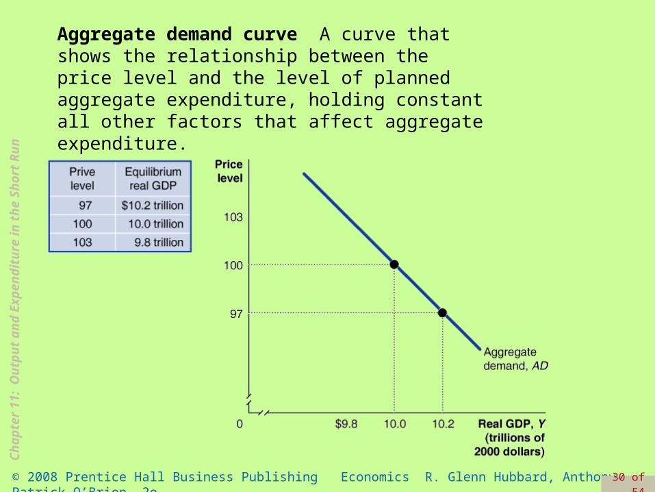
Aggregate demand curve A curve that shows the relationship between the price level and the level of planned aggregate expenditure, holding constant all other factors that affect aggregate expenditure.

Ch
apte
r 11
: O
utp
ut
and
Ex
pen
dit
ure
in
th
e S
ho
rt R
un
© 2008 Prentice Hall Business Publishing Economics R. Glenn Hubbard, Anthony Patrick O’Brien, 2e. 31 of 54
Aggregate demand curve
Aggregate expenditure (AE)
Aggregate expenditure model
Autonomous expenditure
Cash flow
Consumption function
Inventories
K e y T e r m s
Marginal propensity to consume (MPC)
Marginal propensity to save (MPS)
Multiplier
Multiplier effect

Ch
apte
r 11
: O
utp
ut
and
Ex
pen
dit
ure
in
th
e S
ho
rt R
un
© 2008 Prentice Hall Business Publishing Economics R. Glenn Hubbard, Anthony Patrick O’Brien, 2e. 32 of 54
The Algebra of Macroeconomic Equilibrium
Appendix
)(YMPCCC
1I
GG
XNNX
NXGICY
1 Consumption function
2 Planned investment function
3 Government spending function
4 Net export function
5 Equilibrium condition
Ch
apte
r 11
: O
utp
ut
and
Ex
pen
dit
ure
in
th
e S
ho
rt R
un
© 2008 Prentice Hall Business Publishing Economics R. Glenn Hubbard, Anthony Patrick O’Brien, 2e. 33 of 54
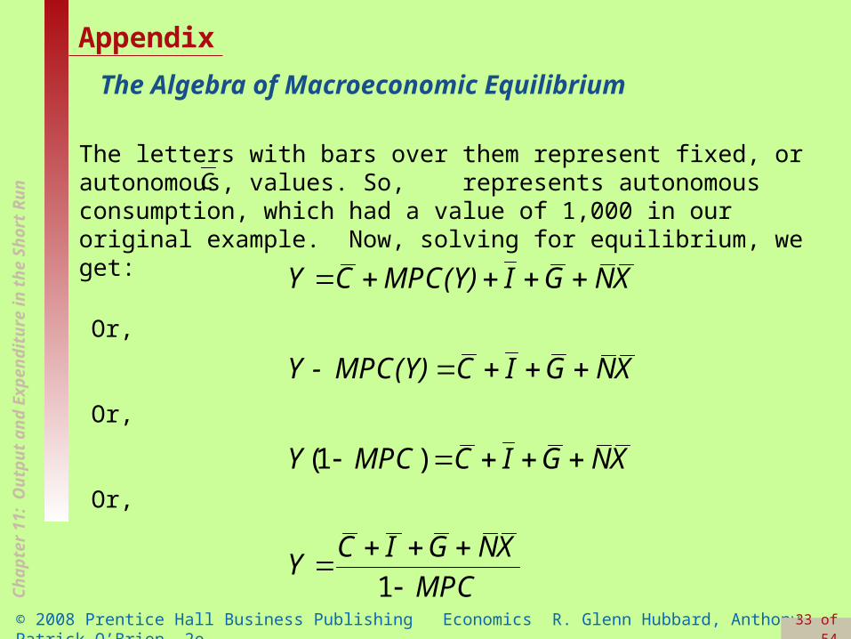
The Algebra of Macroeconomic Equilibrium
Appendix
( )
1
1
Y C MPC(Y) I G NX
Y - MPC(Y) C I G NX
Y MPC C I G NX
C I G NXY
MPC
Or,
Or,
Or,
The letters with bars over them represent fixed, or autonomous, values. So, represents autonomous consumption, which had a value of 1,000 in our original example. Now, solving for equilibrium, we get:
C
Ch
apte
r 11
: O
utp
ut
and
Ex
pen
dit
ure
in
th
e S
ho
rt R
un
© 2008 Prentice Hall Business Publishing Economics R. Glenn Hubbard, Anthony Patrick O’Brien, 2e. 34 of 54
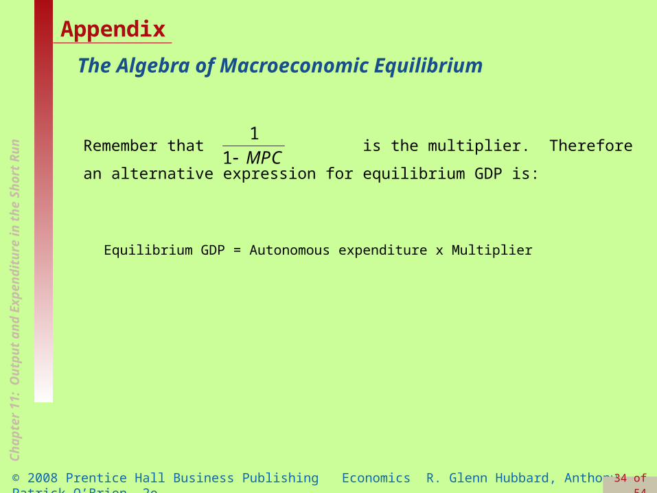
The Algebra of Macroeconomic Equilibrium
Appendix
Remember that is the multiplier. Therefore an alternative
expression for equilibrium GDP is:
1
1 MPC
Equilibrium GDP = Autonomous expenditure x Multiplier
Related Documents


