Chapter 11: Managing Economies of Scale Uncertainty in a the Supply Chain: Safety Inventory Exercise Solutions 1. D L = LD = (2)(300) = 600 σ L = √ L σ D = √ 2( 200 ) = 283 ss = F S -1 (CSL) L = F S -1 (0.95) 283 = 465 (where, F S -1 (0.95) = NORMSINV (0.95)) ROP = DL + ss = 600 + 465 = 1065 Excel Worksheet 11-1 illustrates these computations 2. D L = (T+L) D = (2+3)(300) = 1500 σ L = √ T+L σ D = √ 2+3 ( 200 ) = 447 ss = F S -1 (CSL) L = F S -1 (0.95) 447 = 736 (where, F S -1 (0.95) = NORMSINV (0.95)) OUL = D(T+L) + ss = 1500 + 736 = 2236 Excel Worksheet 11-2 illustrates these computations 3. D L = LD = (2)(300) = 600 σ L = √ L σ D = √ 2( 200 ) = 283 1

Chapter 11 Exercise Answers
Oct 23, 2014
Welcome message from author
This document is posted to help you gain knowledge. Please leave a comment to let me know what you think about it! Share it to your friends and learn new things together.
Transcript

Chapter 11: Managing Economies of ScaleUncertainty in athe Supply Chain: Safety
Inventory
Exercise Solutions
1.
DL = LD = (2)(300) = 600
σ L = √ Lσ D = √2(200 )= 283
ss = FS-1
(CSL) L = FS-1
(0.95) 283 = 465 (where, FS-1
(0.95) = NORMSINV (0.95))
ROP = DL + ss = 600 + 465 = 1065
Excel Worksheet 11-1 illustrates these computations
2.
DL = (T+L) D = (2+3)(300) = 1500
σ L = √T+L σ D = √2+3(200 )= 447
ss = FS-1
(CSL) L = FS-1
(0.95) 447 = 736 (where, FS-1
(0.95) = NORMSINV (0.95))
OUL = D(T+L) + ss = 1500 + 736 = 2236
Excel Worksheet 11-2 illustrates these computations
3.
DL = LD = (2)(300) = 600
σ L = √ Lσ D = √2(200 )= 283
ESC = (1 – fr)Q = (1 – 0.99)500 = 5
We use the following expression to determine the safety stock (ss):
ESC=−ss [ 1−F S(ss
σ L
)]+σ L f S(ss
σ L
)
ESC = –ss[1 – NORMDIST(ss/L, 0, 1, 1)] + L NORMDIST(ss/L, 0, 1, 0).
We utilize the GOALSEEK function in EXCEL in determining safety stock (ss) by using ss as the changing value that results in an ESC value of 5.
1
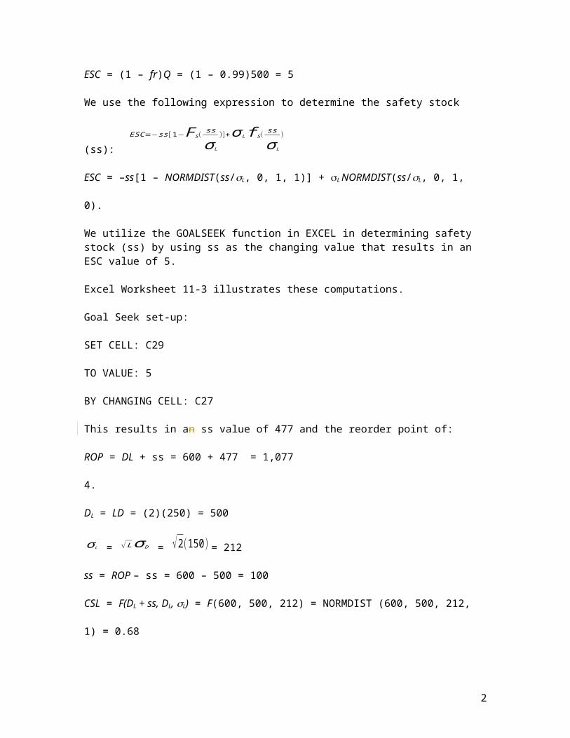
Excel Worksheet 11-3 illustrates these computations.
Goal Seek set-up:
SET CELL: C29
TO VALUE: 5
BY CHANGING CELL: C27
This results in an ss value of 477 and the reorder point of:
ROP = DL + ss = 600 + 477 = 1,077
4.
DL = LD = (2)(250) = 500
σ L = √ Lσ D = √2(150)= 212
ss = ROP – ss = 600 – 500 = 100
CSL = F(DL + ss, DL, L) = F(600, 500, 212) = NORMDIST (600, 500, 212, 1) = 0.68
ESC=−ss [ 1−F S(ss
σ L
)]+σ L f S(ss
σ L
)
ESC = –ss[1 – NORMDIST(ss/L, 0, 1, 1)] + L NORMDIST(ss/L, 0, 1, 0) = 43.86
Fill rate (fr) = 1- (ESC/Q) = 1- (43.86/1000) = 0.96
Excel Worksheet 11-4 illustrates these computations
5.
DL = LD = (2)(250) = 500
L =√ Lσ D
2
+D2
sL
2
= √2×1502
+2502
×1. 52
= 431
ss = FS-1
(CSL) L = FS-1
(0.95) 431 = 709 (where, FS-1
(0.95) = NORMSINV (0.95))
ESC=−ss [ 1−F S(ss
σ L
)]+σ L f S(ss
σ L
)
ESC = –ss[1 – NORMDIST(ss/L, 0, 1, 1)] + L NORMDIST(ss/L, 0, 1, 0) = 9
Fill rate (fr) = 1- (ESC/Q) = 1- (9/1000) = 0.991
2
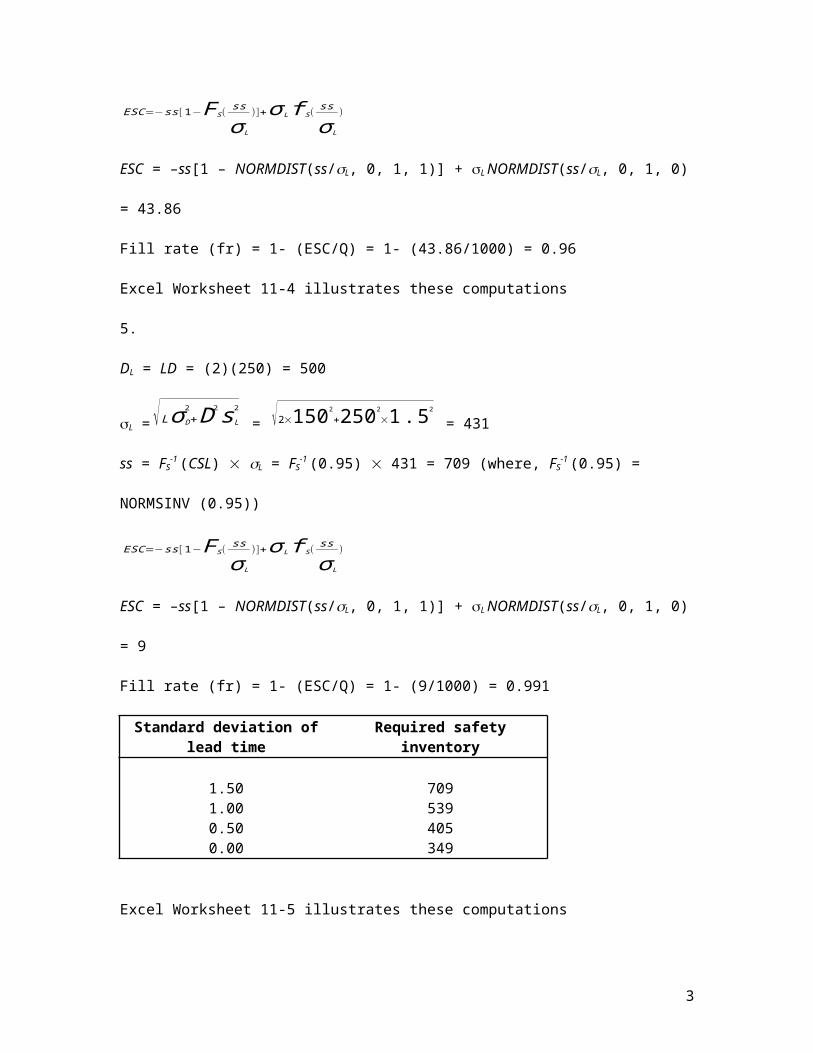
Standard deviation of lead time Required safety inventory
1.50 709 1.00 539 0.50 405 0.00 349
Excel Worksheet 11-5 illustrates these computations
6.
Following are the evaluations for the Khaki pants:
Disaggregated Option:
DL = LD = (4)(800) = 3200
σ L = √ Lσ D = √4 (100)= 200
Coefficient of variation = σ /μ = 100/800 = 0.13
ss per store = FS-1
(CSL) L = FS-1
(0.95) 200 = 329 (where, FS-1
(0.95) = NORMSINV (0.95))
Total safety inventory = (329)(900) = 296,074
Total value of safety inventory = (296,074)(30) = $8,882,210
Total annual safety inventory holding cost = (8,882,210)(0.25) = $2,220,552
Holding cost per unit sold = 2220552/(800)(900) = $3.08
Aggregated Option:
DC
=kD = (900)(800) = 720000
σ D
C
=√k σ = √900(100 )= 3000
DL = LDC = (4)(800)(900) = 2,880,000
σ L = √ L σDC
= √4 (3000)= 6000
ss = FS-1
(CSL) L = FS-1
(0.95) 6000 = 9869 (where, FS-1
(0.95) = NORMSINV (0.95))
Total safety inventory = 9869
3

Total value of safety inventory = (9869)(30) = $296,070
Total annual safety inventory holding cost = (296070 )(0.25) = $74,018
Holding cost per unit sold = 74018/(800)(900) = $0.1
Savings in the holding cost per unit sold from aggregation = $3.08 - $0.1 = $2.98
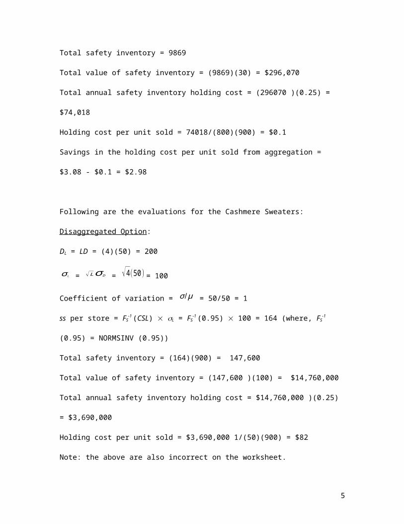
Following are the evaluations for the Cashmere Sweaters:
Disaggregated Option:
DL = LD = (4)(50) = 200
σ L = √ Lσ D = √4 (50)= 100
Coefficient of variation = σ /μ = 50/50 = 1
ss per store = FS-1
(CSL) L = FS-1
(0.95) 100 = 164 (where, FS-1
(0.95) = NORMSINV (0.95))
Total safety inventory = (164)(900) = 147,600
Total value of safety inventory = (147,600 )(100) = $14,760,000
Total annual safety inventory holding cost = $14,760,000 )(0.25) = $3,690,000
Holding cost per unit sold = $3,690,000 1/(50)(900) = $82
Note: the above are also incorrect on the worksheet.
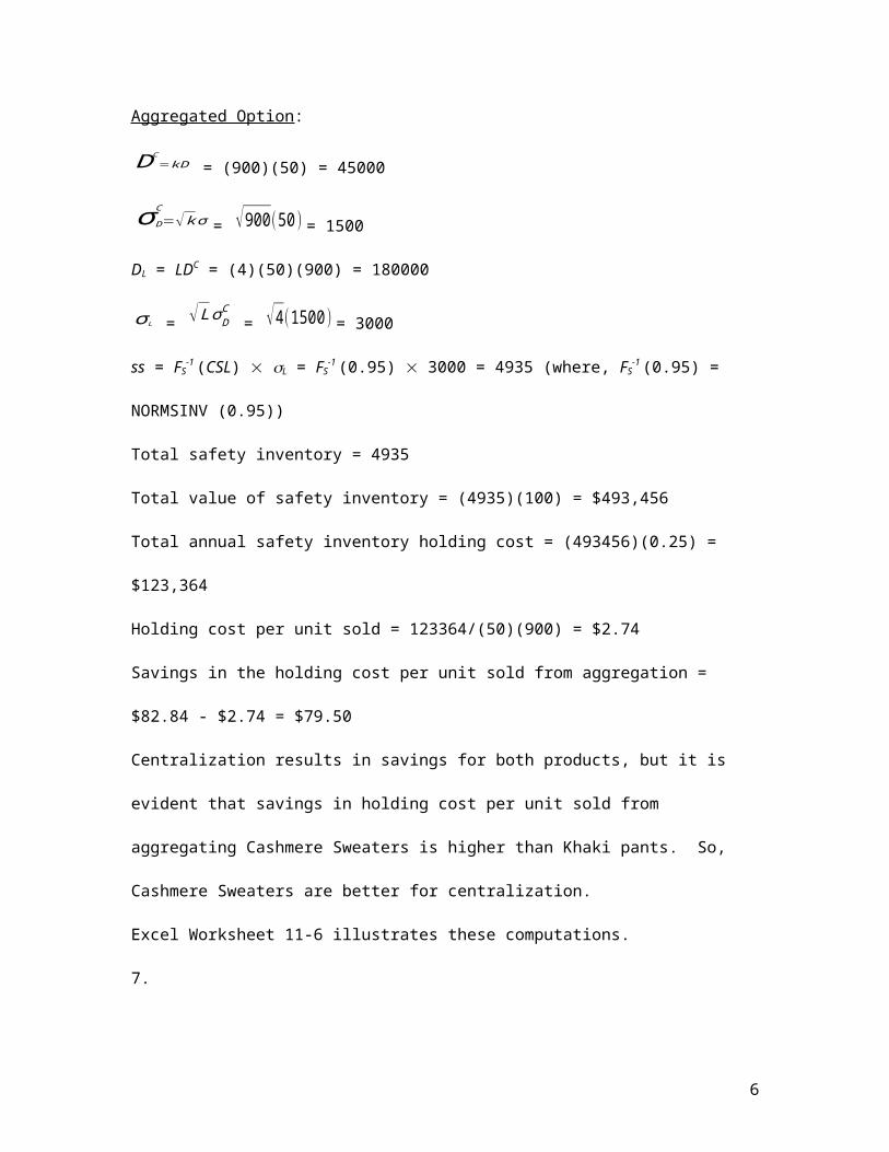
Aggregated Option:
DC
=kD = (900)(50) = 45000
σ D
C
=√k σ = √900(50 )= 1500
DL = LDC = (4)(50)(900) = 180000
σ L = √ L σDC
= √4 (1500)= 3000
ss = FS-1
(CSL) L = FS-1
(0.95) 3000 = 4935 (where, FS-1
(0.95) = NORMSINV (0.95))
Total safety inventory = 4935
Total value of safety inventory = (4935)(100) = $493,456
4
Total annual safety inventory holding cost = (493456)(0.25) = $123,364
Holding cost per unit sold = 123364/(50)(900) = $2.74
Savings in the holding cost per unit sold from aggregation = $82.84 - $2.74 = $79.50
Centralization results in savings for both products, but it is evident that savings in holding cost
per unit sold from aggregating Cashmere Sweaters is higher than Khaki pants. So, Cashmere
Sweaters are better for centralization.
Excel Worksheet 11-6 illustrates these computations.
7.
Disaggregated Option:
France:
DL = LD = (8)(3000) = 24000
σ L = √ Lσ D = √82000= 5657
ss at France = FS-1
(CSL) L = FS-1
(0.95) 5657 = 9305
(where, FS-1
(0.95) = NORMSINV (0.95))
The ss at the other five countries is evaluated in a similar manner, which results in a total ss for
Europe of 48,384
Aggregated Option:
DC
=∑i=1
6
D i = 3000 + 4000 + 2000 + 2500+ 1000 + 4000 = 16500
σ D
C
=√∑i=1
6
σ i2
= √20002+22002+14002+16002+8002+24002= 4445.22
DL = LDC = (8)(16500) = 132,000
σ L = √ L σDC
= √8( 4445.22)= 12573
ss = FS-1
(CSL) L = FS-1
(0.95) 12573 = 20,681 (where, FS-1
(0.95) = NORMSINV (0.95))
5
Inventory savings from aggregation = 48,384 – 20,681= 27,704
Excel Worksheet 11-7 illustrates these computations.
8.
(a)
Disaggregated Option:
From the previous problem, we know that the total ss for Europe is 48,384
Holding cost = (200)(0.25)(48384) = $2,419,200
Aggregated Option:
ss = 20,681
Holding cost = (200)(0.25)(20681) = $1,034,036
Savings from aggregation = $2,419,200 -$1,034,036 = $1,385,164
(b) If the $5/unit additional cost of assembly from centralization then the total additional costs = (132000)(52)(5) = Savings = $1,385,164 - So, it is not economical to aggregate
(c) If the lead time changes to 4 weeks, we evaluate the safety stocks and associated costs in a similar manner.
The holding cost from the disaggregated option = (200)(0.25)(34213) = $1,710,650
The holding cost from the aggregated option = (200)(0.25)(14623) = $731,150
Savings from aggregation = $1,710,650 - $731,150 = $979,500
Excel Worksheet 11-8 illustrates these computations.
9.
Since the demand at various locations is not independent, we utilize the following expressions for the aggregated option:
DC = ∑i=1
k D i
var ( DC
)=∑i=1
k
σ i
2
+2∑i> j
ρij σ i σ j
σ D
C
=√ var ( DC
)
6

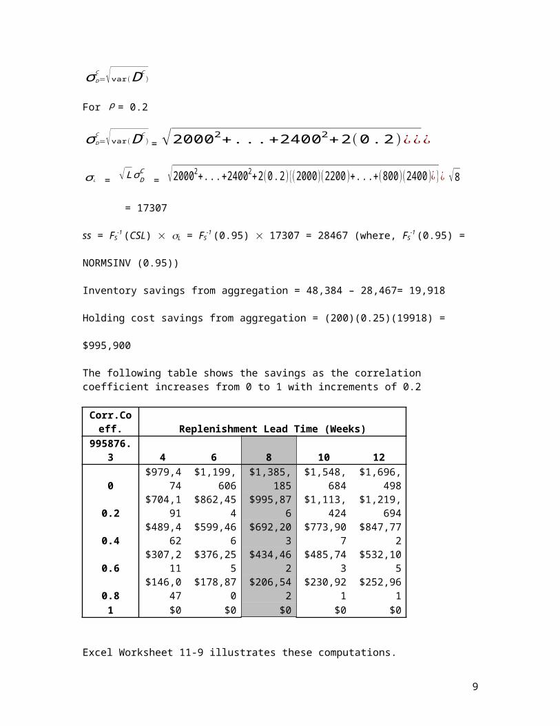
For ρ = 0.2
σ D
C
=√ var ( DC
)=√20002+. . .+24002+2(0 . 2)¿¿¿
σ L = √ L σDC
= √20002+. . .+24002+2(0 . 2){(2000)(2200 )+. ..+(800)(2400 )¿}¿√8
= 17307
ss = FS-1
(CSL) L = FS-1
(0.95) 17307 = 28467 (where, FS-1
(0.95) = NORMSINV (0.95))
Inventory savings from aggregation = 48,384 – 28,467= 19,918
Holding cost savings from aggregation = (200)(0.25)(19918) = $995,900
The following table shows the savings as the correlation coefficient increases from 0 to 1 with increments of 0.2
Corr.Coeff. Replenishment Lead Time (Weeks)
995876.3 4 6 8 10 12
0 $979,47
4$1,199,60
6$1,385,18
5$1,548,68
4$1,696,49
8
0.2 $704,19
1 $862,454 $995,876$1,113,42
4$1,219,69
4
0.4 $489,46
2 $599,466 $692,203 $773,907 $847,772
0.6 $307,21
1 $376,255 $434,462 $485,743 $532,105
0.8 $146,04
7 $178,870 $206,542 $230,921 $252,961
1 $0 $0 $0 $0 $0
Excel Worksheet 11-9 illustrates these computations.
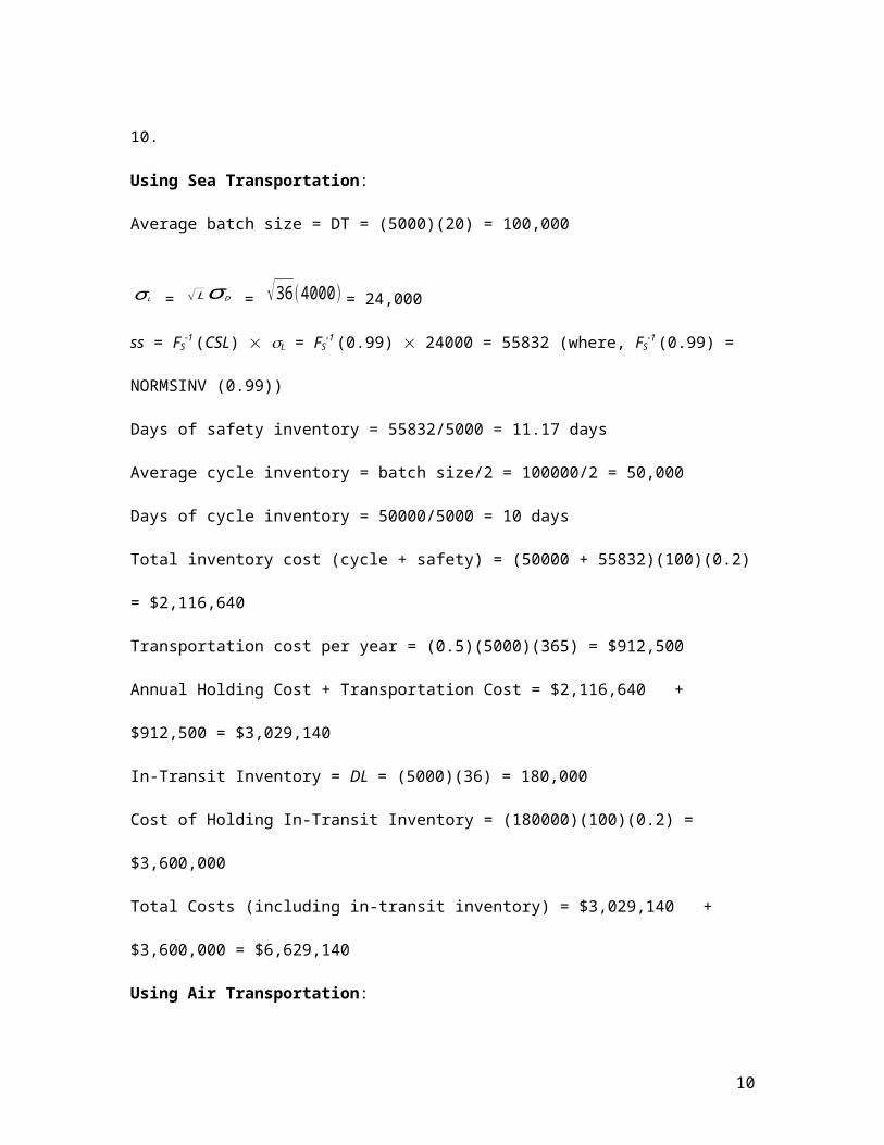
10.
Using Sea Transportation:
Average batch size = DT = (5000)(20) = 100,000
σ L = √ Lσ D = √36( 4000)= 24,000
ss = FS-1
(CSL) L = FS-1
(0.99) 24000 = 55832 (where, FS-1
(0.99) = NORMSINV (0.99))
Days of safety inventory = 55832/5000 = 11.17 days
7

Average cycle inventory = batch size/2 = 100000/2 = 50,000
Days of cycle inventory = 50000/5000 = 10 days
Total inventory cost (cycle + safety) = (50000 + 55832)(100)(0.2) = $2,116,640
Transportation cost per year = (0.5)(5000)(365) = $912,500
Annual Holding Cost + Transportation Cost = $2,116,640 + $912,500 = $3,029,140
In-Transit Inventory = DL = (5000)(36) = 180,000
Cost of Holding In-Transit Inventory = (180000)(100)(0.2) = $3,600,000
Total Costs (including in-transit inventory) = $3,029,140 + $3,600,000 = $6,629,140
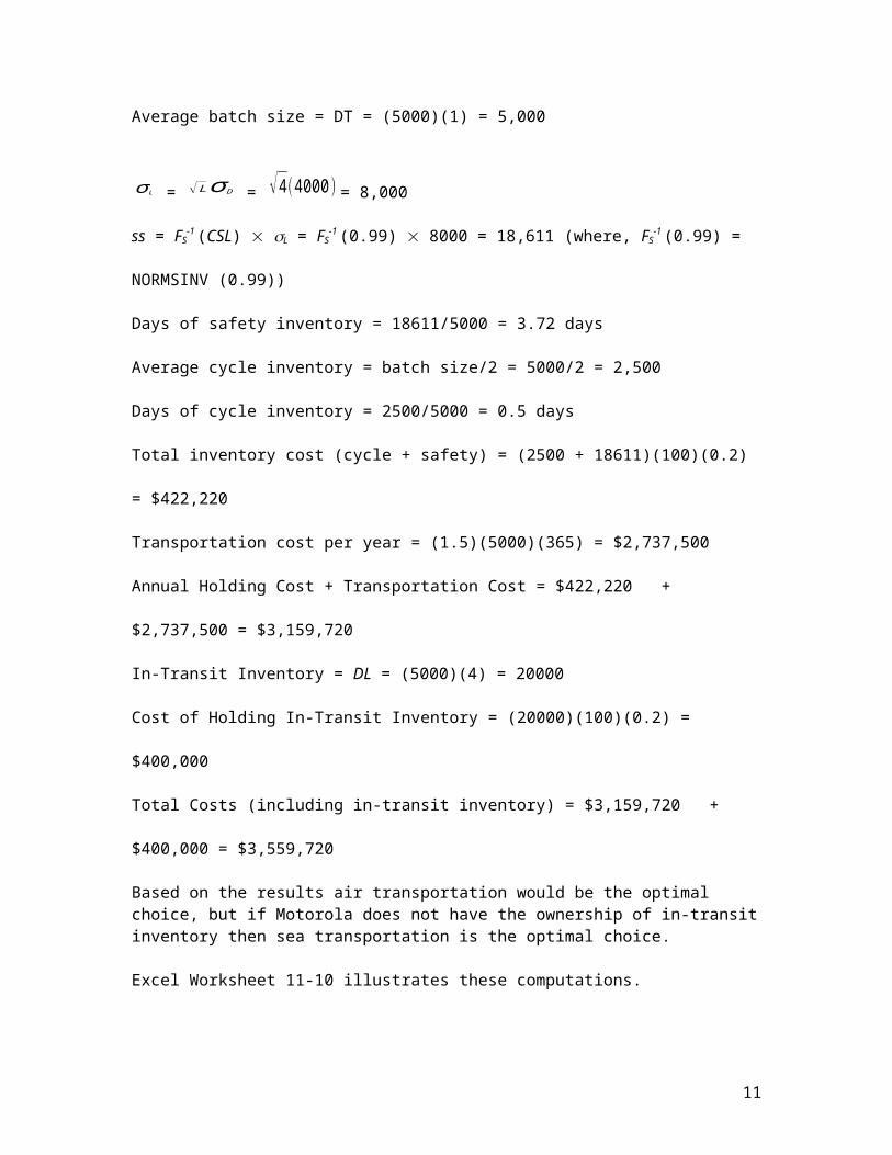
Using Air Transportation:
Average batch size = DT = (5000)(1) = 5,000
σ L = √ Lσ D = √4 (4000 )= 8,000
ss = FS-1
(CSL) L = FS-1
(0.99) 8000 = 18,611 (where, FS-1
(0.99) = NORMSINV (0.99))
Days of safety inventory = 18611/5000 = 3.72 days
Average cycle inventory = batch size/2 = 5000/2 = 2,500
Days of cycle inventory = 2500/5000 = 0.5 days
Total inventory cost (cycle + safety) = (2500 + 18611)(100)(0.2) = $422,220
Transportation cost per year = (1.5)(5000)(365) = $2,737,500
Annual Holding Cost + Transportation Cost = $422,220 + $2,737,500 = $3,159,720
In-Transit Inventory = DL = (5000)(4) = 20000
Cost of Holding In-Transit Inventory = (20000)(100)(0.2) = $400,000
Total Costs (including in-transit inventory) = $3,159,720 + $400,000 = $3,559,720
Based on the results air transportation would be the optimal choice, but if Motorola does not have the ownership of in-transit inventory then sea transportation is the optimal choice.
Excel Worksheet 11-10 illustrates these computations.
8
9
11.
Using Sea Transportation:
Average batch size = DT = (5000)(20) = 100,000
σ L = √ L+T σ D = √36+20( 4000)= 29,933
ss = FS-1
(CSL) L = FS-1
(0.99) 29933 = 69,635 (where, FS-1
(0.99) = NORMSINV (0.99))
Days of safety inventory = 69635/5000 = 13.93 days
OUL = D(T+L) + ss = 5000(36+20) + 69635 = 349,635
Average cycle inventory = batch size/2 = 100000/2 = 50,000
Days of cycle inventory = 50000/5000 = 10 days
Total inventory cost (cycle + safety) = (50000 + 69635)(100)(0.2) = $2,392,700
Transportation cost per year = (0.5)(5000)(365) = $912,500
Annual Holding Cost + Transportation Cost = $2,392,700 + $912,500 = $3,305,200
In-Transit Inventory = DL = (5000)(36) = 180,000
Cost of Holding In-Transit Inventory = (180000)(100)(0.2) = $3,600,000
Total Costs (including in-transit inventory) = $3,029,140 + $3,600,000 = $6,905,200
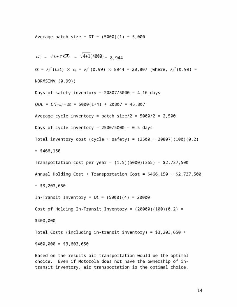
Using Air Transportation:
Average batch size = DT = (5000)(1) = 5,000
σ L = √ L+T σ D = √4+1(4000 )= 8,944
ss = FS-1
(CSL) L = FS-1
(0.99) 8944 = 20,807 (where, FS-1
(0.99) = NORMSINV (0.99))
Days of safety inventory = 20807/5000 = 4.16 days
OUL = D(T+L) + ss = 5000(1+4) + 20807 = 45,807
Average cycle inventory = batch size/2 = 5000/2 = 2,500
Days of cycle inventory = 2500/5000 = 0.5 days
Total inventory cost (cycle + safety) = (2500 + 20807)(100)(0.2) = $466,150
10
Transportation cost per year = (1.5)(5000)(365) = $2,737,500
Annual Holding Cost + Transportation Cost = $466,150 + $2,737,500 = $3,203,650
In-Transit Inventory = DL = (5000)(4) = 20000
Cost of Holding In-Transit Inventory = (20000)(100)(0.2) = $400,000
Total Costs (including in-transit inventory) = $3,203,650 + $400,000 = $3,603,650
Based on the results air transportation would be the optimal choice. Even if Motorola does not have the ownership of in-transit inventory, air transportation is the optimal choice.
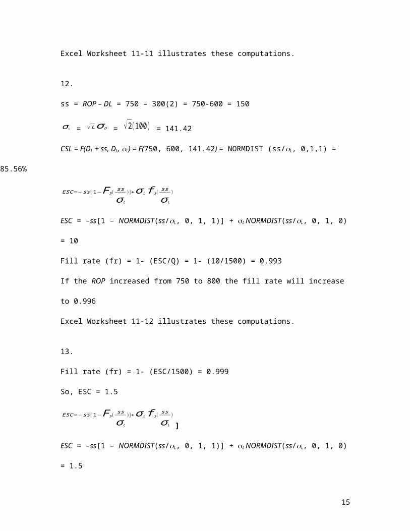
Excel Worksheet 11-11 illustrates these computations.
12.
ss = ROP – DL = 750 – 300(2) = 750-600 = 150
σ L = √ Lσ D = √2(100) = 141.42
CSL = F(DL + ss, DL, L) = F(750, 600, 141.42) = NORMDIST (ss/L, 0,1,1) = 85.56%
ESC=−ss [ 1−F S (ss
σ L
)]+σ L f S (ss
σ L
)
ESC = –ss[1 – NORMDIST(ss/L, 0, 1, 1)] + L NORMDIST(ss/L, 0, 1, 0) = 10
Fill rate (fr) = 1- (ESC/Q) = 1- (10/1500) = 0.993
If the ROP increased from 750 to 800 the fill rate will increase to 0.996
Excel Worksheet 11-12 illustrates these computations.
13.
Fill rate (fr) = 1- (ESC/1500) = 0.999
So, ESC = 1.5
ESC=−ss [ 1−F S(ss
σ L
)]+σ L f S(ss
σ L
)
]
ESC = –ss[1 – NORMDIST(ss/L, 0, 1, 1)] + L NORMDIST(ss/L, 0, 1, 0) = 1.5
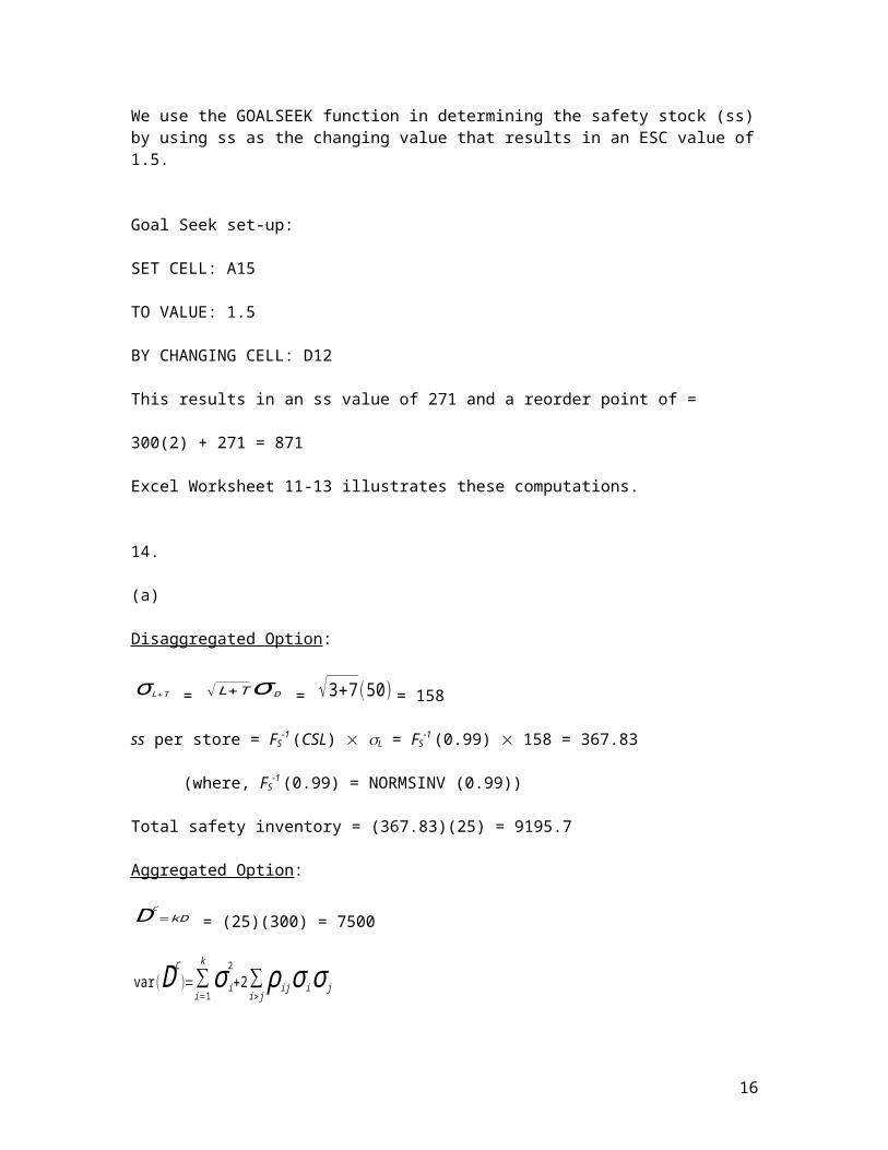
We use the GOALSEEK function in determining the safety stock (ss) by using ss as the changing value that results in an ESC value of 1.5.
11

Goal Seek set-up:
SET CELL: A15
TO VALUE: 1.5
BY CHANGING CELL: D12
This results in an ss value of 271 and a reorder point of = 300(2) + 271 = 871
Excel Worksheet 11-13 illustrates these computations.
14.
(a)
Disaggregated Option:
σ L+T = √ L+T σ D = √3+7(50 )= 158
ss per store = FS-1
(CSL) L = FS-1
(0.99) 158 = 367.83
(where, FS-1
(0.99) = NORMSINV (0.99))
Total safety inventory = (367.83)(25) = 9195.7
Aggregated Option:
DC
=kD = (25)(300) = 7500
var ( DC
)=∑i=1
k
σ i
2
+2∑i> j
ρij σ i σ j
σ D
C
=√ var ( DC
)
σ D
C
=√k σ = √25(50 )= 250 (we are assuming that ρ = 0. If ρ is not 0 then the covariance terms have to be included)
σ L+T = √ L+T σ DC
= √3+7(250 )= 791
ss = FS-1
(CSL) L = FS-1
(0.99) 791 = 1839.14 (where, FS-1
(0.99) = NORMSINV (0.99))
Units savings from aggregation = 9195.7 – 1839.14 = 7356.56
12

Inventory savings = (7356.56) (10) = $73,566
Annual holding cost savings = (73,566 )(0.2) = $14,712
Increase in delivery cost = (300)(25)(365)(0.02) = $54,750
Since the increase in transportation costs outweighs the savings received from aggregation, we do not recommend aggregation for this case.
(b)
We utilize the same approach as in (a) by changing the daily demand mean and standard deviation to 5 and 4, respectively
Units savings from aggregation = 735.66 – 147.13 = 588.52
Inventory savings = (588.52) (10) = $ 5885.2
Annual holding cost savings = ($5885.2 )(0.2) = $1177
Increase in delivery cost = (5)(25)(365)(0.02) = $913
Since the increase in transportation costs does not outweigh the savings received from aggregation, we recommend aggregation for this case.
(c) Yes. The benefit from aggregation decreases as ρ increases. When ρ = 0.5, we do not recommend aggregation in both cases.
Excel Worksheet 11-14 illustrates these computations.
15.
(a)
Popular Variant at Large Dealer:
Decentralized:
ss (at each large dealer) = FS-1
(CSL) √ Lσ D = FS-1
(0.95) √4 (15)= 49.35ss (across all large dealers) = (5)(49.35) = 246.73
Popular Variant at Small Dealer:
Decentralized:
ss (at each small dealer) = FS-1
(CSL) √ Lσ D = FS-1
(0.95) √4 (5)= 16.45ss (across all small dealers) = (30)(16.45) = 493.46
(b )
Popular Variant all Inventories Centralized:
13
Demand per period = demand at large dealers + demand at small dealers = (50)(5) + (10)(30) = 550
Standard deviation of demand per period = √5(15 )2+30(5 )2= 43.30
ss (at regional warehouse) = FS-1
(CSL) √ Lσ D = FS-1
(0.95) √4 (43 .30)= 142.45
reduction in safety inventory from complete aggregation = 246.73 + 493.46 – 142.45 = 597.74
holding cost savings per year = (597.74)(20000)(0.2) = $2,390,942.52
production + transportation cost increase per year = (550)(100)(52) = $2,860,000
(c)
Popular Variant only Small Dealer Inventories Centralized:
Demand per period = demand at small dealers = (10)(30) = 300
Standard deviation of demand per period = √30(5 )2= 27.39
ss (at regional warehouse) = FS-1
(CSL) √ Lσ D = FS-1
(0.95) √4 (27 .39 )= 90.09
reduction in safety inventory from small dealer centralization = 493.46 – 90.09 = 403.36
holding cost savings per year = (403.36)(20000)(0.2) = $1,613,440
production + transportation cost increase per year = (300)(100)(52) = $1,560,000
(d) Centralizing inventories from small dealers and decentralizing at large dealers is the optimal strategy
(e) Similar analysis can be performed for the uncommon variant (See EXCEL worksheet 11-15 for more details)
(f) For the popular variant, centralize inventories from small dealers and decentralize at large dealers. For the uncommon variant, centralize all inventories.
Excel Worksheet 11-15 illustrates these computations.
16.
High volume variant without component commonality:
ss (for the variant) = FS-1
(CSL) √ Lσ D = FS-1
(0.95) √4 (200)= 657.94ss (across all high volume variants) = (1)(657.94) = 657.94
14
Low volume variant without component commonality:
ss (for the variant) = FS-1
(CSL) √ Lσ D = FS-1
(0.95) √4 (20)= 65.79ss (across all low volume variants) = (9)(65.79) = 592.15
(b & c)
With complete commonality:
Demand per period = demand for high volume variant + demand for low volume variant = (1000)(1) + (28)(9) = 1252
Standard deviation of demand per period = √1(200)2+9(20 )2= 208.81
ss = FS-1
(CSL) √ Lσ D = FS-1
(0.95) 8686.91
reduction in safety inventory from complete commonality = 657.94 + 592.15 – 686.91 = 563.18
holding cost savings per year = (563.18)(1000)(0.2) = $112,635.54
component cost increase per period = (1252)(25)(52) = $1,627,600
additional cost at which complete commonality is justified = 112635.54/(1252)(52) = $1.73
Commonality is not justified across all variants because of increased costs.
(d & e)
Only low volume variant uses commonality
Demand per period = demand for low volume variant = (28)(9) = 252
Standard deviation of demand per period = √9(20 )2= 60
ss = FS-1
(CSL) √ Lσ D = FS-1
(0.95) √4 (60 )= 197.38
reduction in safety inventory from low volume variant using commonality = 592.15 – 197.38 = 394.76
holding cost savings per year = (394.76)(1000)(0.2) = $78,952.97
component cost increase per period = (252)(25)(52) = $327,600
additional cost at which complete commonality is justified = 78952.97/(252)(52) = $6.03
Commonality is not justified across low volume variants because of increased costs.
15
Excel Worksheet 11-16 illustrates these computations.
16
Related Documents