Chapter 11

BPS - 5th Ed. Chapter 11 1

Chapter 11

Sampling Distributions


Sampling Terminology Parameter

– fixed, unknown number that describes the population Statistic

– known value calculated from a sample– a statistic is often used to estimate a parameter

Variability– different samples from the same population may yield

different values of the sample statistic Sampling Distribution

– tells what values a statistic takes and how often it takes those values in repeated sampling


Parameter vs. Statistic

A properly chosen sample of 1600 people across the United States was asked if they regularly watch a certain television program, and 24% said yes. The parameter of interest here is the true proportion of all people in the U.S. who watch the program, while the statistic is the value 24% obtained from the sample of 1600 people.


Parameter vs. Statistic

The mean of a population is denoted by µ – this is a parameter.

The mean of a sample is denoted by – this is a statistic. is used to estimate µ.

xx

The true proportion of a population with a certain trait is denoted by p – this is a parameter.

The proportion of a sample with a certain trait is denoted by (“p-hat”) – this is a statistic. is used to estimate p.

p̂ p̂


The Law of Large Numbers

Consider sampling at random from a population with true mean µ. As the number of (independent) observations sampled increases, the mean of the sample gets closer and closer to the true mean of the population.

( gets closer to µ ) x


The Law of Large NumbersGambling

The “house” in a gambling operation is not gambling at all– the games are defined so that the gambler has a

negative expected gain per play (the true mean gain after all possible plays is negative)

– each play is independent of previous plays, so the law of large numbers guarantees that the average winnings of a large number of customers will be close the the (negative) true average


Sampling Distribution The sampling distribution of a statistic

is the distribution of values taken by the statistic in all possible samples of the same size (n) from the same population– to describe a distribution we need to specify

the shape, center, and spread– we will discuss the distribution of the sample

mean (x-bar) in this chapter


Case Study

Does This Wine Smell Bad?

Dimethyl sulfide (DMS) is sometimes present in wine, causing “off-odors”. Winemakers want to know the odor threshold – the lowest concentration of DMS that the human nose can detect. Different people have different thresholds, and of interest is the mean threshold in the population of all adults.


Case Study

Suppose the mean threshold of all adults is =25 micrograms of DMS per liter of wine, with a standard deviation of =7 micrograms per liter and the threshold values follow a bell-shaped (normal) curve.



Where should 95% of all individual threshold values fall?

mean plus or minus two standard deviations

25 2(7) = 11

25 + 2(7) = 39

95% should fall between 11 & 39

What about the mean (average) of a sample of n adults? What values would be expected?


Sampling Distribution What about the mean (average) of a sample of

n adults? What values would be expected? Answer this by thinking: “What would happen if we

took many samples of n subjects from this population?” (let’s say that n=10 subjects make up a sample)

– take a large number of samples of n=10 subjects from the population

– calculate the sample mean (x-bar) for each sample– make a histogram (or stemplot) of the values of x-bar– examine the graphical display for shape, center, spread


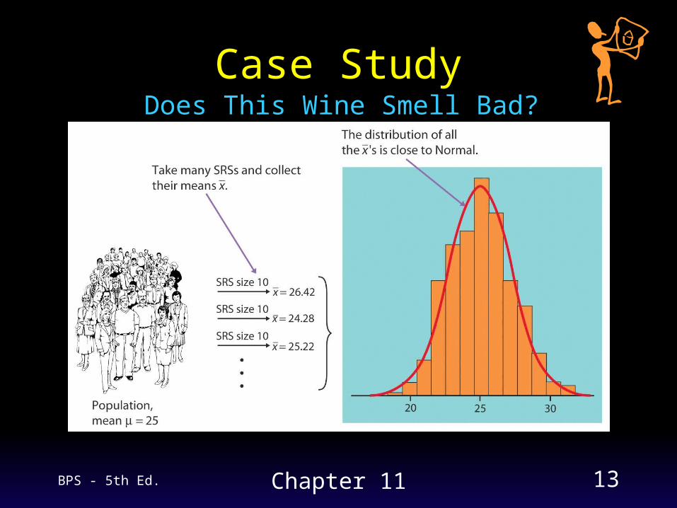
Case Study

Mean threshold of all adults is =25 micrograms per liter, with a standard deviation of =7 micrograms per liter and the threshold values follow a bell-shaped (normal) curve.

Many (1000) repetitions of sampling n=10 adults from the population were simulated and the resulting histogram of the 1000x-bar values is on the next slide.



Case StudyDoes This Wine Smell Bad?


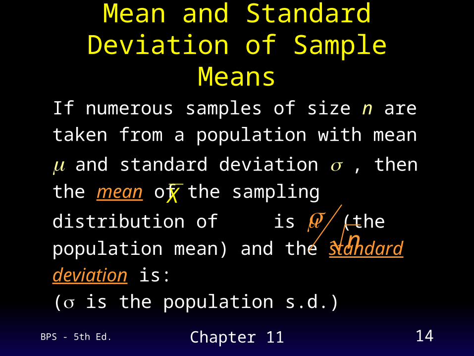
Mean and Standard Deviation of Sample Means

If numerous samples of size n are taken from

a population with mean and standard

deviation , then the mean of the sampling

distribution of is (the population mean)

and the standard deviation is:

( is the population s.d.) n

X


Mean and Standard Deviation of Sample Means

Since the mean of is , we say that is

an unbiased estimator of X X

Individual observations have standard deviation , but sample means from samples of size n have standard deviation

. Averages are less variable than individual observations.

X

n


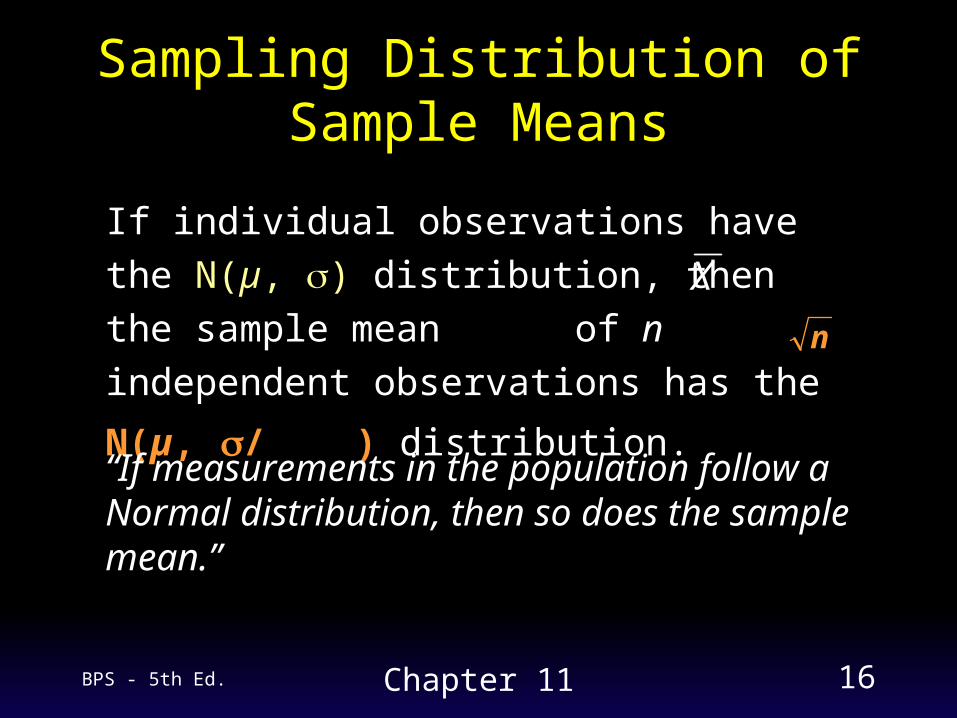
Sampling Distribution ofSample Means

If individual observations have the N(µ, )

distribution, then the sample mean of n

independent observations has the N(µ, / )

distribution.

X

n

“If measurements in the population follow a Normal distribution, then so does the sample mean.”


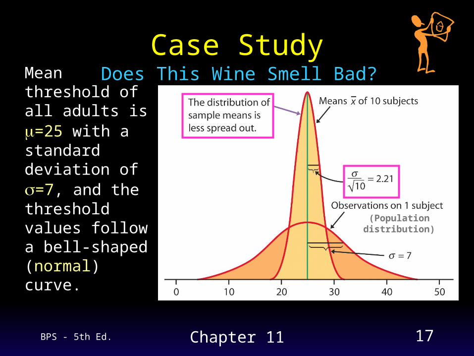
Case Study

Mean threshold of all adults is =25 with a standard deviation of =7, and the threshold values follow a bell-shaped (normal) curve.


(Population distribution)


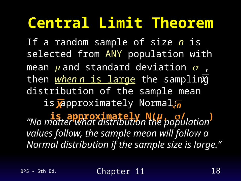
Central Limit Theorem

“No matter what distribution the population values follow, the sample mean will follow a Normal distribution if the sample size is large.”

If a random sample of size n is selected from ANY population with mean and standard

deviation , then when n is large the sampling distribution of the sample mean is approximately Normal:

is approximately N(µ, / )

X

nX


Central Limit Theorem:Sample Size

How large must n be for the CLT to hold?– depends on how far the population

distribution is from Normal the further from Normal, the larger the sample

size needed a sample size of 25 or 30 is typically large

enough for any population distribution encountered in practice

recall: if the population is Normal, any sample size will work (n≥1)


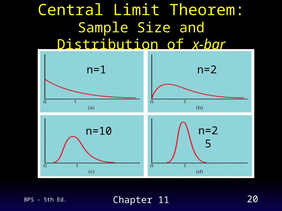
Central Limit Theorem:Sample Size and Distribution of x-bar

n=1

n=25n=10

n=2


Statistical Process Control

Goal is to make a process stable over time and keep it stable unless there are planned changes

All processes have variation Statistical description of stability over time:

the pattern of variation remains stable (does not say that there is no variation)


Statistical Process Control A variable described by the same distribution

over time is said to be in control To see if a process has been disturbed and

to signal when the process is out of control, control charts are used to monitor the process– distinguish natural variation in the process from

additional variation that suggests a change

– most common application: industrial processes


Charts There is a true mean that describes the

center or aim of the process Monitor the process by plotting the means

(x-bars) of small samples taken from the process at regular intervals over time

Process-monitoring conditions:– measure quantitative variable x that is Normal– process has been operating in control for a long period– know process mean and standard deviation that

describe distribution of x when process is in control

x


Control Charts Plot the means (x-bars) of regular samples of

size n against time Draw a horizontal center line at

x

Draw horizontal control limits at ± 3/ n– almost all (99.7%) of the values of x-bar should be

within the mean plus or minus 3 standard deviations

Any x-bar that does not fall between the control limits is evidence that the process is out of control


Case Study

Need to control the tension in millivolts (mV) on the mesh of fine wires behind the surface of the screen.

– Proper tension is 275 mV (target mean )

– When in control, the standard deviation of the tension readings is =43 mV

Making Computer Monitors


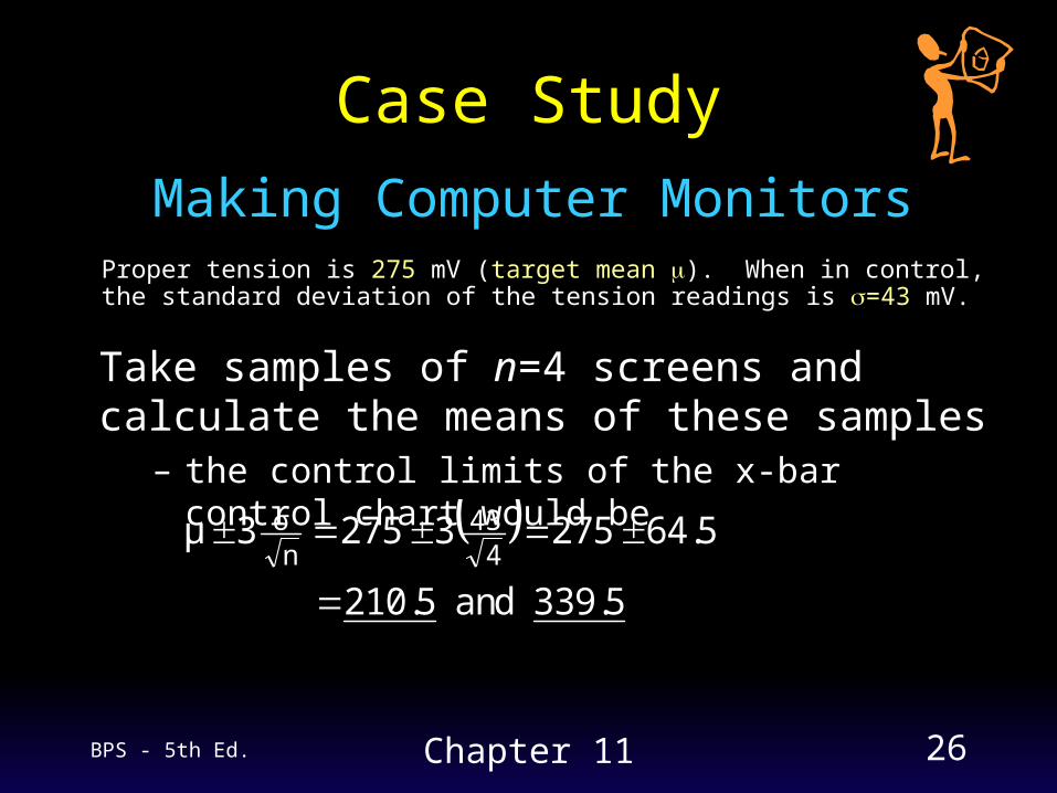
Case Study

Proper tension is 275 mV (target mean ). When in control, the standard deviation of the tension readings is =43 mV.


Take samples of n=4 screens and calculate the means of these samples

– the control limits of the x-bar control chart would be

339.5 and 210.5

64.527532753μ4

43n

σ


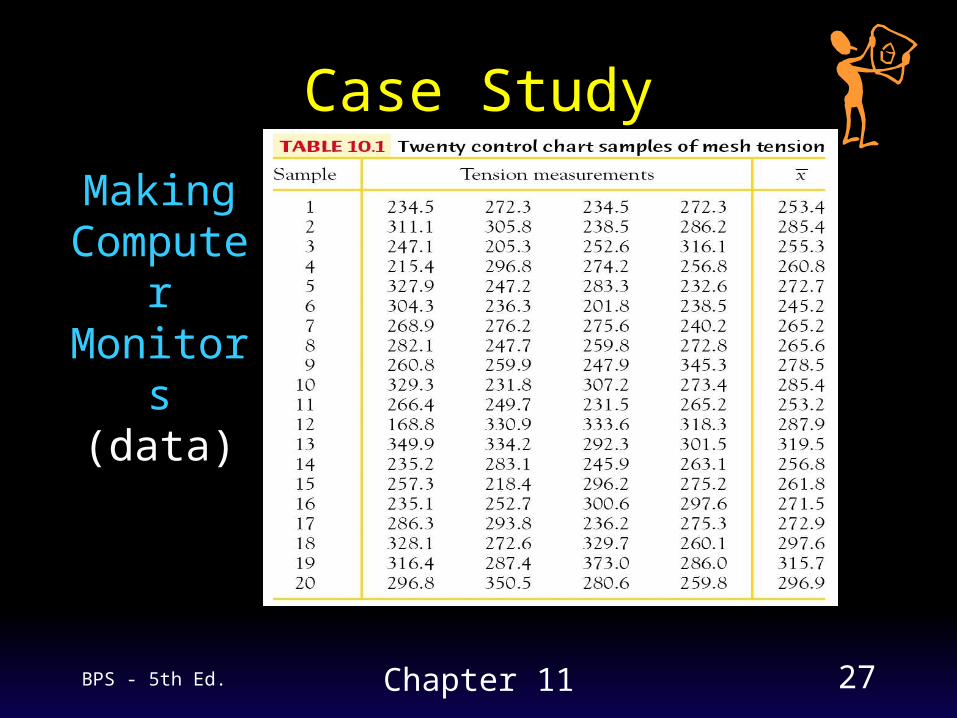
Case Study


(data)


Case Study

Making Computer Monitors( chart)x

(in control)


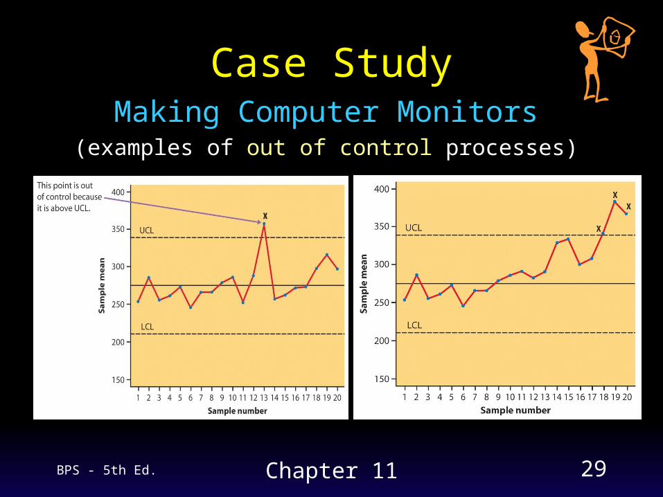
Case StudyMaking Computer Monitors

(examples of out of control processes)


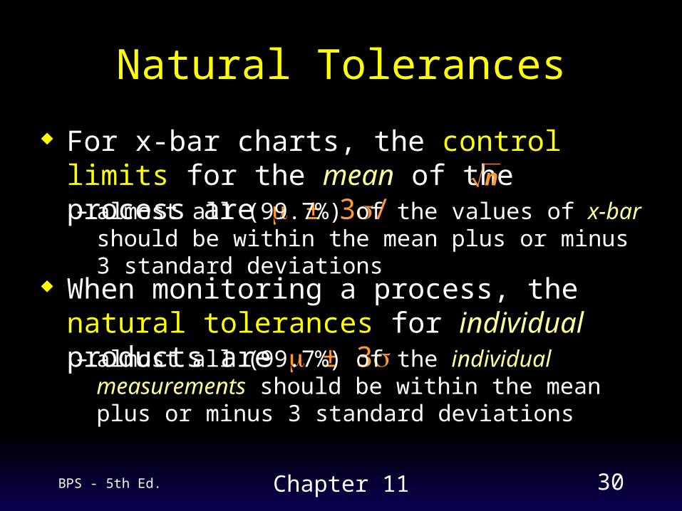
Natural Tolerances

For x-bar charts, the control limits for the mean of the process are ± 3/ n

– almost all (99.7%) of the values of x-bar should be within the mean plus or minus 3 standard deviations

When monitoring a process, the natural tolerances for individual products are ± 3– almost all (99.7%) of the individual measurements

should be within the mean plus or minus 3 standard deviations

Chapter 11

Documents

sampling distributions

mean threshold

mean average

true mean gain

distribution of values

different values

sample mean xbar

sample of n adults