Chapter 10 Sinusoidal Steady-State Power Calculations · 2015-11-30 · 1/30/2014 1 Chapter 10 Sinusoidal Steady-State Power Calculations In Chapter 9, we calculated the steady state

1/30/2014

1

Chapter 10 Sinusoidal Steady-State Power Calculations

In Chapter 9, we calculated the steady state voltages and currents in electric circuits driven by sinusoidal sources.

We used phasor method to find the steady state voltages and currents.

In this chapter, we consider power in such circuits.

The techniques we develop are useful for analyzing many of the electric devices we encounter daily, because sinusoidal sources are predominate means of providing electric power in our homes, school, and businesses.

Examples are:Electric Heater which transform electric energy to thermal energyElectric Stove and ovenToastersIron Electric water heater

And many others

10.1 Instantaneous Power

Consider the following circuit represented by a black box.

( )i t

( )v t

( ) cos( )m ii t I t

( ) cos( )vmv t V t

The instantaneous power assuming passive sign convention

( Current in the direction of voltage drop )

(( ) ( ))v tp t i t ( Watts )

If the current is in the direction of voltage rise ( ) the instantaneous power is:

(( ) ( ))vp tt i t

( )i t

( )v t

1/30/2014

2

( )i t

( )v t

( ) cos( )m ii t I t

( ) cos( )vmv t V t

(( ) ( ))v tp t i t cos( ){ }{ cos }( )mivmV t I t

cos( cos( ) )m vm iI tV t

1 12

cos cos cos( ) cos2

( ) Since

Therefore

( ) cos( )mi t I t

( ) cos( )v imv t V t

cos( ) cos cos sin ins Since

cos(2 ) cos( )cos(2 ) sin( )sin(2 )v vi i ivt t t

( ) cos( ) cos( )cos(2 ) sin( )sin(2 )2 2 2

m m mv v v

m m mi i i

I I Ip t t V tV V

( ) cos( ) cos(2 ) 2 2

mi iv

mmv

mI Ip t tV V

( )i t

( )v t

( ) cos( )mi t I t

( ) cos( )v imv t V t

( ) cos( ) cos( cos() sin( )2 2 2

sin(2 ) 2 )m m mi i

m m mv v v i tI It V Vp V t I

o o 0= 0 =6v i

You can see that that the frequency of the Instantaneouspower is twice the frequency of the voltage or current

1/30/2014

3

10.2 Average and Reactive Power

( ) cos( ) cos( cos() sin( )2 2 2

sin(2 ) 2 )m m mi i

m m mv v v i tI It V Vp V t I

Recall the Instantaneous power p(t)

cos( si( ) ) n ) (2 2p t tt P P Q

where

cos( ) 2

mi

mv

IP V Average Power (Real Power)

sin( ) 2

mi

mv

IQ V Reactive Power

Average Power P is sometimes called Real power because it describes the power in a circuit that is transformed from electric to non electric ( Example Heat ).

It is easy to see why P is called Average Power because

0

0

t +1 ( )t

Tp t dt

T 0

0

cos(t +1 { }sin(2) )t

2T

P P Q t dtT

t P

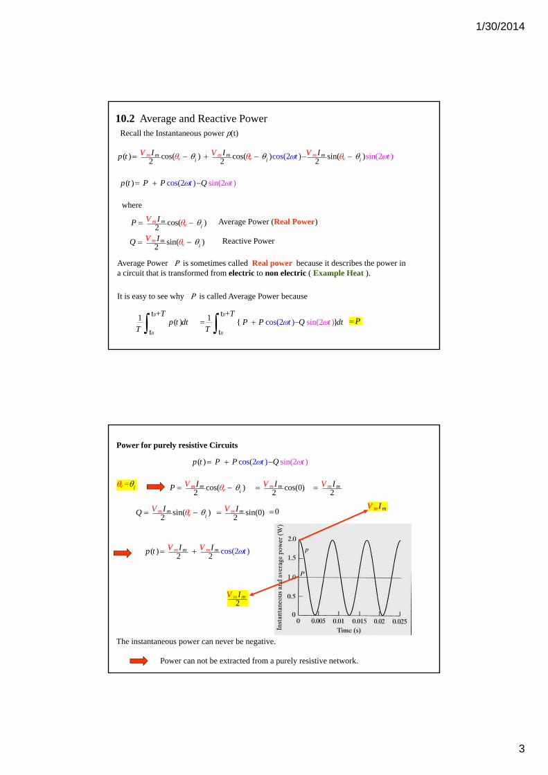
Power for purely resistive Circuits

( ) cos(22 2

)m mm mI Ip t tV V

= iv cos( ) 2

mi

mv

IP V

sin( ) 2

mi

mv

IQ V

2

mmV I

0

c os(0) 2

m mV I

s in(0) 2

m mV I

The instantaneous power can never be negative.

cos( si( ) ) n ) (2 2p t tt P P Q

mmV I

2mmV I

Power can not be extracted from a purely resistive network.

1/30/2014

4

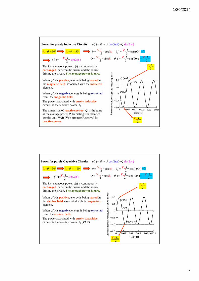
Power for purely Inductive Circuits

sin(2 )( ) 2

m mIp Vt t

o9= 0iv cos( ) 2

mi

mv

IP V

sin( ) 2

mi

mv

IQ V 2

mmV I

0cos(90 ) 2

om mV I

sin(90 ) 2

om mV I

cos( si( ) ) n )(2 2p t tt P P Q

2mmV I

2mmV I

o= 90 v i

The instantaneous power p(t) is continuously exchanged between the circuit and the source driving the circuit. The average power is zero.

When p(t) is positive, energy is being stored in the magnetic field associated with the inductiveelement.

When p(t) is negative, energy is being extractedfrom the magnetic field.

The power associated with purely inductivecircuits is the reactive power Q.

The dimension of reactive power Q is the same as the average power P. To distinguish them we use the unit VAR (Volt Ampere Reactive) for reactive power.

Power for purely Capacitive Circuits

( )2

sin(2 )m mV Ip t t

o9= 0iv cos( ) 2

mi

mv

IP V

sin( ) 2

mi

mv

IQ V 2

mmV I

0ocos( 9 )2

0 m mIV

sin( 9 2

0 )m omIV

cos( si( ) ) n )(2 2p t tt P P Q

2mmV I

2mmV I

o= 90v i

The instantaneous power p(t) is continuously exchanged between the circuit and the source driving the circuit. The average power is zero.

When p(t) is positive, energy is being stored in the electric field associated with the capacitiveelement.

When p(t) is negative, energy is being extractedfrom the electric field.

The power associated with purely capacitivecircuits is the reactive power Q (VAR).

1/30/2014

5

The power factor

( ) cos( ) c

s

os( ) sin in( )2 2 2

c (os(2 )

2

)m m mm m miv v vi i

I I Ip t

P P

V tV

Q

t V

average averagepower po

reactivepw o erer w

Recall the Instantaneous power p(t)

cos( sin(2 2 ) ) tQtP P

The angle v i plays a role in the computation of both average and reactive power

The angle v i is referred to as the power factor angle

We now define the following :

The power factor cos( )v i pf

The reactive factor sin( )v i rf

The power factor cos( )v i pf

Knowing the power factor pf does not tell you the power factor angle, because

cos( ) cos( )i viv

To completely describe this angle, we use the descriptive phrases lagging power factorand leading power factor

Lagging power factor implies that current lags voltage hence an inductive load

Leading power factor implies that current leads voltage hence a capacitive load

1/30/2014

6

10.3 The rms Value and Power Calculations

Rcos( )m v

V t

Assume that a sinusoidal voltage is applied to the terminals of a resistor as shown

Suppose we want to determine the average power delivered to the resistor

0

0

t +1 ( )t

TP p t dt

T

0

0

cos2

( )t +1 t

tv

VTm dt

RT

0

0

2 2t +1 1 cos ( )

t m

TV dt

Rt

T v

However since0

0

2 2t +1 cos ( )rmst m

TV V dt

T vt

2

rms

VP

R If the resistor carry sinusoidal current 2

rmsP RI

Recall the Average and Reactive power

cos( ) 2

mi

mv

IP V sin( ) 2

mi

mv

IQ V

Which can be written as

cos( ) 2 2

mv i

mV IP sin( ) 2 2

mv i

mV IQ

Therefore the Average and Reactive power can be written in terms of the rms value as

s rmsrm cos( ) v iP V I sin( ) rms vrms iQ V I

The rms value is also referred to as the effective value eff

Therefore, the average and reactive power can be written in terms of the eff value as:

f effef cos( ) v iP V I f effef sin( ) v iQ V I

1/30/2014

7

Example 10.3

10.4 Complex Power

Previously, we found it convenient to introduce sinusoidal voltage and current in terms of the complex number, the phasor.

Definition

were is the complex power is the reactive p

is the average poweerr

ow

P

Q

j

P

Q S

S

Let the complex power be the complex sum of real power and reactive power

1/30/2014

8

Advantages of using complex power

{ }P S { }Q S

We can compute the average and reactive power from the complex power S

complex power S provide a geometric interpretation

QjP S

QjP SS

( )Q

reactive power

( )

Paverage power

cos( )tan

sin( )vm

vm

m i

m i

IVIV

2 2= P QS

n =taQP

e j S

where

cos( )tan

sin( )v i

iv

tan tan( )v i iv

power factor angle

The geometric relations for a right triangle mean the four power triangle dimensions (|S|, P, Q, ) can be determined if any two of the four are known.

is called the apparent power

Example 10.4

1/30/2014

9

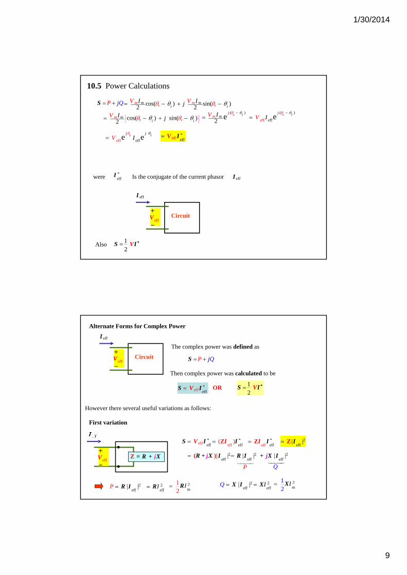
10.5 Power Calculations

QjP S cos( ) sin( )2 2

m mi i

m mv v

V VI Ij

cos( ) sin( )2

mv v

mi i

I jV

( )

2 e

j ivmmV I eff

( )

eff e ivjV I

eff

eff e evj j iIV

eff*eff

V I

were*eff

I Is the conjugate of the current phasor effI

effV

effI

Circuit

Also1 2

*S VI

Alternate Forms for Complex Power

effV

effI

Circuit

1 2

*S VI

eff*eff

S IV

The complex power was defined as

QjP S

Then complex power was calculated to be

OR

However there several useful variations as follows:

First variation

eff*eff

( ) Z II

eff*eff

S IV

eff*eff

Z II 2eff

| | Z I

2eff

| | ( )+ X IjReffV

Z = +R jX 2 2

eff eff| | | | + X IjR I

P

Q

2eff

| |P R I 2eff

I R 2m

1 2

I R2

eff| |Q X I 2

eff I X 2

m 12

I X

1/30/2014

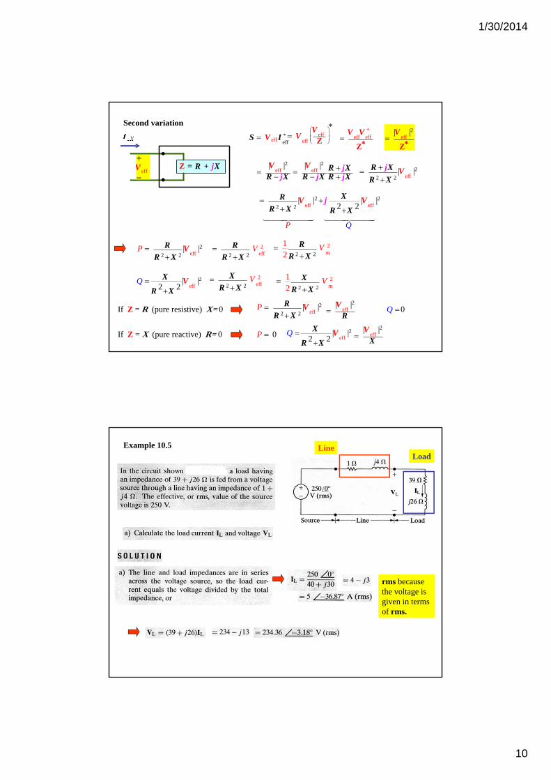
10

eff*eff

S IV

Second variationeff

eff

*

Z

VV

*eff eff

*Z

V Veff

2

| |

*Z

V

eff2|

|

V

R jXeffV

Z = +R jX

P

e2

ff | |

jR XVR X Rj jX

2

2 e2 ff | |

R X

R XVj

eff e2 2

2 2 ff | | | |

2 2

V Vj XR

R X R X

Q

2

2 2 eff| |P

R XVR

e2

ff| |

2 2Q

VX

R X

2 2

2eff

VR

R X

2m

2 2

1 2

VR

R X

2 2

2eff

VX

R X2

m

2 2

1 2

VX

R X

If Z = R (pure resistive) X= 0 2

2 2 eff| |P

R XVR

eff2|

|

V

R0Q

If Z = X (pure reactive) R= 0 0P e2

ff| |

2 2Q

VX

R Xeff

2|

|

VX

Example 10.5 LineLoad

rms because the voltage is given in termsof rms.

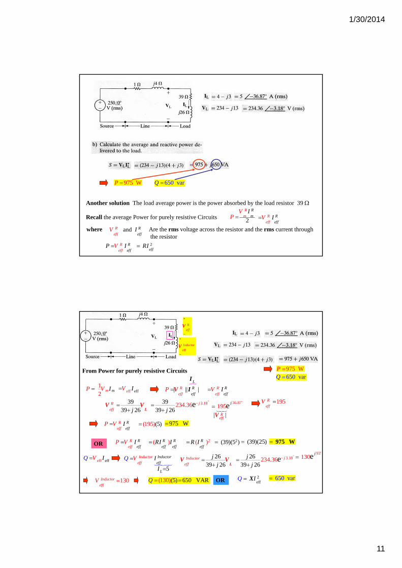
1/30/2014

11

975 WP 650 varQ

Another solution The load average power is the power absorbed by the load resistor 39

Recall the average Power for purely resistive Circuits

where and R

f

R

eff efIV Are the rms voltage across the resistor and the rms current through

the resistor 2 eff

RI

2

R R

m mV

PI

R

feff

R

e fIV

R R

eeff ffP IV

975 WP 650 varQ

2(39)(5 ) (39)(25) 975 W

| || |R

ff ffe

R

eP IV

3939 26

R

eff j

LV V

o36.87195e j

195R

effV

R R

eeff ffP IV (195 ))(5 975 W

OR R R

eeff ffP IV ( )R R

eff effRI I 2( )R

effR I

o

3.18234.399 2

363 6

e j

j

5

Inductor

eff

Inductor

eff

L

Q IV

I

2639 26

Inductor

eff

jj

L

V Vo

3.182342639 6

.362

e jjj

o93 130e j

130Inductor

effV (5)(1 630 5 VA) 0 RQ OR 650 var2

eff IQ X

R

eff

V

| | Reff

V

R

feff

R

e fIV

From Power for purely resistive Circuits

2 1 mmP V I efeff f IV

LI

eff eff VQ I

Inductor

eff

V

1/30/2014

12

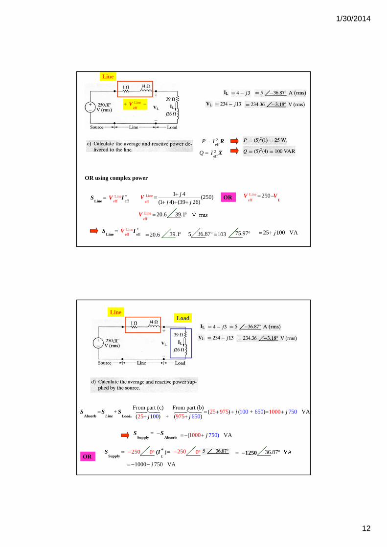
Line

2eff

P I R

2eff

Q I X

Lineeff

*eff

Line

IVS

Line

eff V

Line

eff

1 4 (250)(1 4) (39 26)

jj j

V OR Line

eff250

LV V

o39.1Line

eff20.6V

Lineeff

*eff

Line

IVS o39.120.6 o36.875 103 o75.97 25 100 VAj

OR using complex power

LineLoad

+Absorb Line Load

S S S100

From part (c) From part (b)

( ) + ( )25 97 6505j j ( ) (1025 9 07 6 05 )5+ j 751 000 VA0 j

OR

7( VA10 0 0 50) j = Supply Absorb

S S

1000 750 VAj

250Supply

S o0 )L

*(I 250 o0 1250 o36.87

1/30/2014

13

Example 10.6 Calculating Power in Parallel Loads

cos( )v i pf

1/30/2014

14

6 000 V 8 A000 j 1

S1 6000 V1 A2000 j

2S 10000 V20000 Aj S

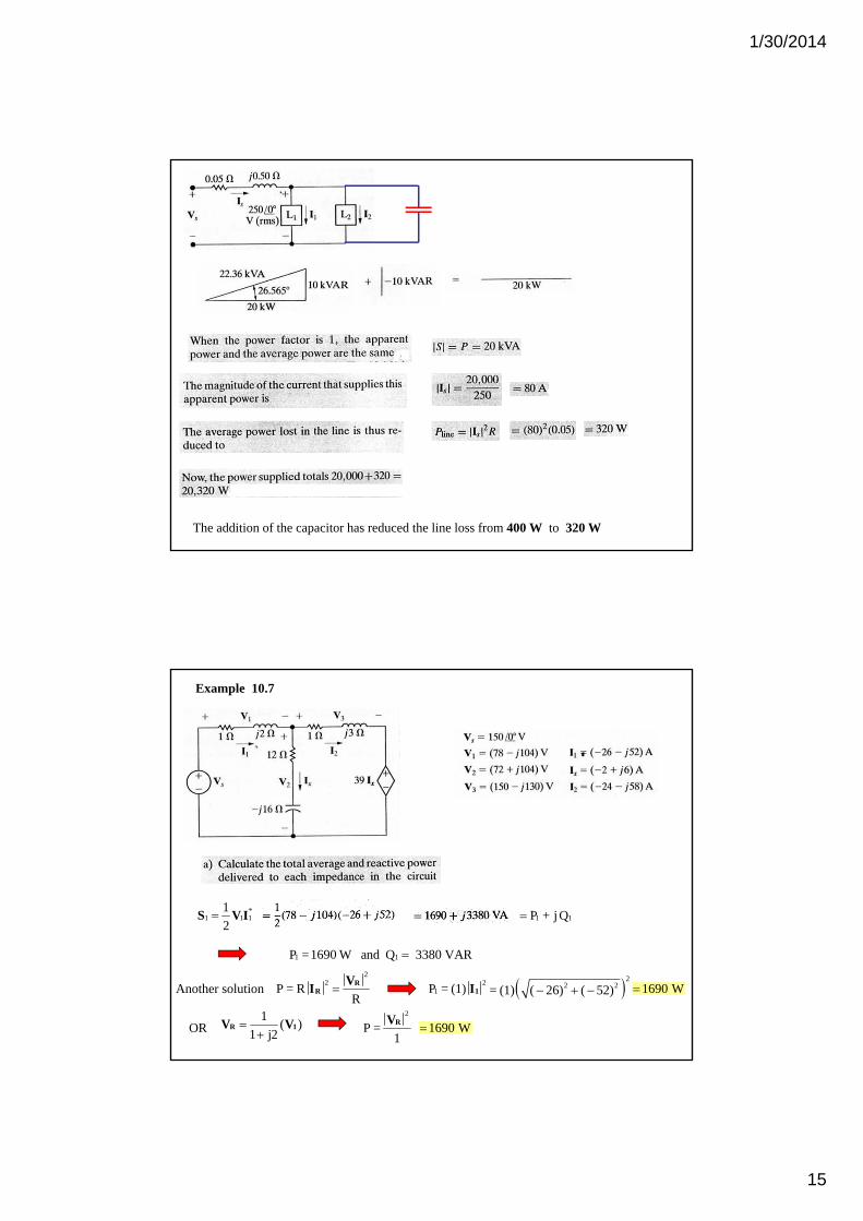
The apparent power which must be supplied to these loads is

20000| | | 100 VA 00| j S 22.36 kVA

C ?

| |S

As we can see from the power triangle

We can correct the power factor to 1

Recall that 1XC

if we place a capacitor in parallel with the existing load

Will cancel this

1/30/2014

15

The addition of the capacitor has reduced the line loss from 400 W to 320 W

Example 10.7

*1 1 1

1

2S V I 1 1P + j Q

1 1P = 1690 W and Q 3380 VAR

Another solution2

2P = R

R R

RV

I2

1P = (1) 1I 22 2= (1) ( 26) ( 52) 1690 W

1( )

1 j2

R 1V VOR

2

P = 1RV

1690 W

1/30/2014

16

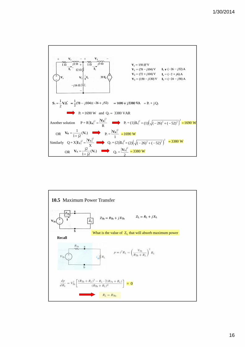
*1 1 1

1

2S V I 1 1P + j Q

1 1P = 1690 W and Q 3380 VAR

Another solution2

2P = R

R R

RV

I2

1P = (1) 1I 22 2= (1) ( 26) ( 52) 1690 W

1( )

1 j2

R 1V VOR

2

1P = 1RV

1690 W

Similarly2

2Q = X

X X

XV

I2

1Q = (2) 1I 22 2= (2) ( 26) ( 52) 3380 W

j2( )

1 j2

X 1V VOR

2

1Q = 2XV 3380 W

= 0

What is the value of ZL that will absorb maximum powerRecall

10.5 Maximum Power Transfer

1/30/2014

17

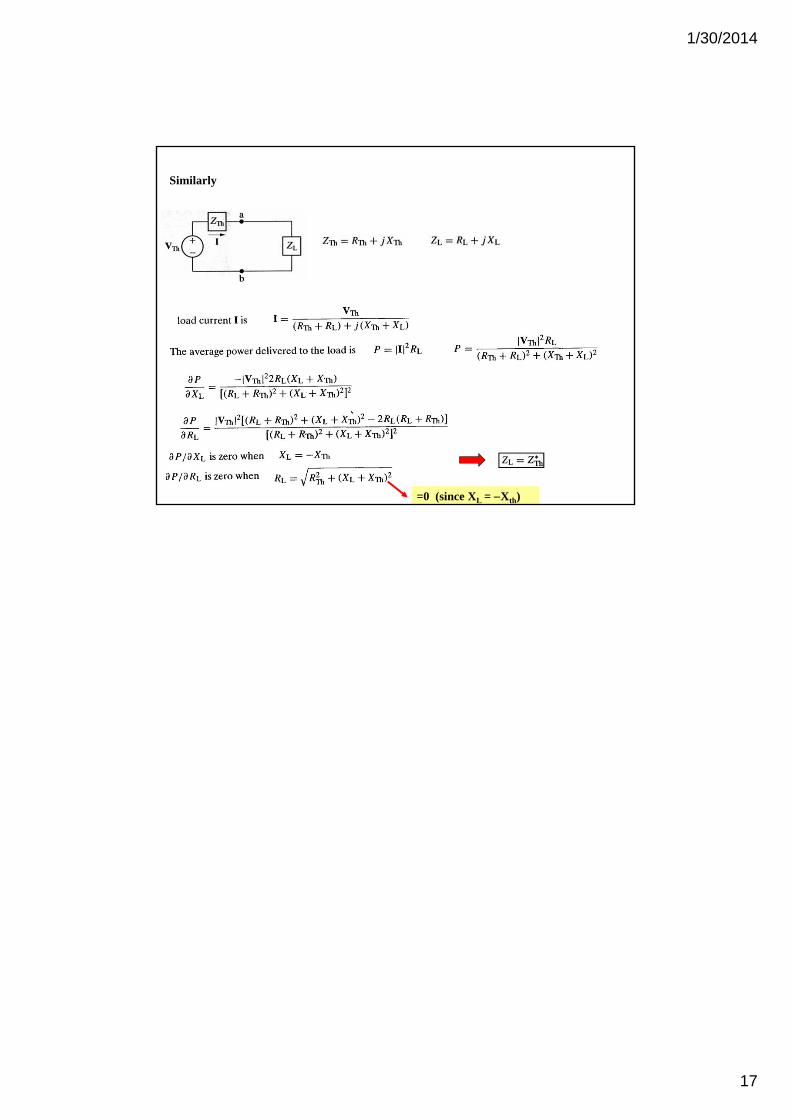
Similarly

=0 (since XL = Xth)