CHAPTER 10 Part-of-Speech Tagging · particle A particle resembles a preposition or an adverb and is used in combination with a verb. Particles often have extended meanings that aren’t

Speech and Language Processing. Daniel Jurafsky & James H. Martin. Copyright c© 2016. All

rights reserved. Draft of November 7, 2016.

CHAPTER

10 Part-of-Speech Tagging

Conjunction Junction, what’s your function?Bob Dorough, Schoolhouse Rock, 1973

A gnostic was seated before a grammarian. The grammarian said, ‘A word mustbe one of three things: either it is a noun, a verb, or a particle.’ The gnostic tore hisrobe and cried, ‘Alas! Twenty years of my life and striving and seeking have gone tothe winds, for I laboured greatly in the hope that there was another word outside ofthis. Now you have destroyed my hope.’ Though the gnostic had already attained theword which was his purpose, he spoke thus in order to arouse the grammarian.

Rumi (1207–1273), The Discourses of Rumi, Translated by A. J. Arberry

Dionysius Thrax of Alexandria (c. 100 B.C.), or perhaps someone else (exact author-ship being understandably difficult to be sure of with texts of this vintage), wrote agrammatical sketch of Greek (a “techne”) that summarized the linguistic knowledgeof his day. This work is the source of an astonishing proportion of modern linguisticvocabulary, including words like syntax, diphthong, clitic, and analogy. Also in-cluded are a description of eight parts-of-speech: noun, verb, pronoun, preposition,parts-of-speech

adverb, conjunction, participle, and article. Although earlier scholars (includingAristotle as well as the Stoics) had their own lists of parts-of-speech, it was Thrax’sset of eight that became the basis for practically all subsequent part-of-speech de-scriptions of Greek, Latin, and most European languages for the next 2000 years.

Schoolhouse Rock was a popular series of 3-minute musical animated clips firstaired on television in 1973. The series was designed to inspire kids to learn multi-plication tables, grammar, basic science, and history. The Grammar Rock sequence,for example, included songs about parts-of-speech, thus bringing these categoriesinto the realm of popular culture. As it happens, Grammar Rock was remarkablytraditional in its grammatical notation, including exactly eight songs about parts-of-speech. Although the list was slightly modified from Thrax’s original, substitutingadjective and interjection for the original participle and article, the astonishing dura-bility of the parts-of-speech through two millenia is an indicator of both the impor-tance and the transparency of their role in human language. Nonetheless, eight isn’tvery many and more recent part-of-speech tagsets have many more word classes,tagset

like the 45 tags used by the Penn Treebank (Marcus et al., 1993).Parts-of-speech (also known as POS, word classes, or syntactic categories)POS

are useful because of the large amount of information they give about a word andits neighbors. Knowing whether a word is a noun or a verb tells us a lot aboutlikely neighboring words (nouns are preceded by determiners and adjectives, verbsby nouns) and about the syntactic structure around the word (nouns are generally partof noun phrases), which makes part-of-speech tagging an important component ofsyntactic parsing (Chapter 12). Parts of speech are useful features for finding named

2 CHAPTER 10 • PART-OF-SPEECH TAGGING

entities like people or organizations in text and other information extraction tasks(Chapter 20). Parts-of-speech influence the possible morphological affixes and socan influence stemming for informational retrieval, and can help in summarizationfor improving the selection of nouns or other important words from a document. Aword’s part of speech is important for producing pronunciations in speech synthesisand recognition. The word content, for example, is pronounced CONtent when it isa noun and conTENT when it is an adjective (Chapter 30).

This chapter focuses on computational methods for assigning parts-of-speech towords, part-of-speech tagging. After summarizing English word classes and thepart-of-speech

taggingstandard Penn tagset, we introduce two algorithms for tagging: the Hidden MarkovModel (HMM) and the Maximum Entropy Markov Model (MEMM).

10.1 (Mostly) English Word Classes

Until now we have been using part-of-speech terms like noun and verb ratherfreely. In this section we give a more complete definition of these and other classes.While word classes do have semantic tendencies—adjectives, for example, oftendescribe properties and nouns people— parts-of-speech are traditionally defined in-stead based on syntactic and morphological function, grouping words that have sim-ilar neighboring words (their distributional properties) or take similar affixes (theirmorphological properties).

Parts-of-speech can be divided into two broad supercategories: closed classclosed class

types and open class types. Closed classes are those with relatively fixed member-open class

ship, such as prepositions—new prepositions are rarely coined. By contrast, nounsand verbs are open classes—new nouns and verbs like iPhone or to fax are contin-ually being created or borrowed. Any given speaker or corpus may have differentopen class words, but all speakers of a language, and sufficiently large corpora,likely share the set of closed class words. Closed class words are generally functionwords like of, it, and, or you, which tend to be very short, occur frequently, andfunction word

often have structuring uses in grammar.Four major open classes occur in the languages of the world: nouns, verbs,

adjectives, and adverbs. English has all four, although not every language does.The syntactic class noun includes the words for most people, places, or things, butnoun

others as well. Nouns include concrete terms like ship and chair, abstractions likebandwidth and relationship, and verb-like terms like pacing as in His pacing to andfro became quite annoying. What defines a noun in English, then, are things like itsability to occur with determiners (a goat, its bandwidth, Plato’s Republic), to takepossessives (IBM’s annual revenue), and for most but not all nouns to occur in theplural form (goats, abaci).

Open class nouns fall into two classes. Proper nouns, like Regina, Colorado,proper noun

and IBM, are names of specific persons or entities. In English, they generally aren’tpreceded by articles (e.g., the book is upstairs, but Regina is upstairs). In writtenEnglish, proper nouns are usually capitalized. The other class, common nouns arecommon noun

divided in many languages, including English, into count nouns and mass nouns.count nounmass noun Count nouns allow grammatical enumeration, occurring in both the singular and plu-

ral (goat/goats, relationship/relationships) and they can be counted (one goat, twogoats). Mass nouns are used when something is conceptualized as a homogeneousgroup. So words like snow, salt, and communism are not counted (i.e., *two snowsor *two communisms). Mass nouns can also appear without articles where singular

10.1 • (MOSTLY) ENGLISH WORD CLASSES 3

count nouns cannot (Snow is white but not *Goat is white).The verb class includes most of the words referring to actions and processes,verb

including main verbs like draw, provide, and go. English verbs have inflections(non-third-person-sg (eat), third-person-sg (eats), progressive (eating), past partici-ple (eaten)). While many researchers believe that all human languages have the cat-egories of noun and verb, others have argued that some languages, such as Riau In-donesian and Tongan, don’t even make this distinction (Broschart 1997; Evans 2000;Gil 2000) .

The third open class English form is adjectives, a class that includes many termsadjective

for properties or qualities. Most languages have adjectives for the concepts of color(white, black), age (old, young), and value (good, bad), but there are languageswithout adjectives. In Korean, for example, the words corresponding to Englishadjectives act as a subclass of verbs, so what is in English an adjective “beautiful”acts in Korean like a verb meaning “to be beautiful”.

The final open class form, adverbs, is rather a hodge-podge, both semanticallyadverb

and formally. In the following sentence from Schachter (1985) all the italicizedwords are adverbs:

Unfortunately, John walked home extremely slowly yesterday

What coherence the class has semantically may be solely that each of thesewords can be viewed as modifying something (often verbs, hence the name “ad-verb”, but also other adverbs and entire verb phrases). Directional adverbs or loca-tive adverbs (home, here, downhill) specify the direction or location of some action;locative

degree adverbs (extremely, very, somewhat) specify the extent of some action, pro-degree

cess, or property; manner adverbs (slowly, slinkily, delicately) describe the mannermanner

of some action or process; and temporal adverbs describe the time that some ac-temporal

tion or event took place (yesterday, Monday). Because of the heterogeneous natureof this class, some adverbs (e.g., temporal adverbs like Monday) are tagged in sometagging schemes as nouns.

The closed classes differ more from language to language than do the openclasses. Some of the important closed classes in English include:

prepositions: on, under, over, near, by, at, from, to, withdeterminers: a, an, thepronouns: she, who, I, othersconjunctions: and, but, or, as, if, whenauxiliary verbs: can, may, should, areparticles: up, down, on, off, in, out, at, bynumerals: one, two, three, first, second, third

Prepositions occur before noun phrases. Semantically they often indicate spatialpreposition

or temporal relations, whether literal (on it, before then, by the house) or metaphor-ical (on time, with gusto, beside herself), but often indicate other relations as well,like marking the agent in (Hamlet was written by Shakespeare,

A particle resembles a preposition or an adverb and is used in combination withparticle

a verb. Particles often have extended meanings that aren’t quite the same as theprepositions they resemble, as in the particle over in she turned the paper over.

When a verb and a particle behave as a single syntactic and/or semantic unit, wecall the combination a phrasal verb. Phrasal verbs cause widespread problems withphrasal verb

natural language processing because they often behave as a semantic unit with a non-compositional meaning— one that is not predictable from the distinct meanings ofthe verb and the particle. Thus, turn down means something like ‘reject’, rule outmeans ‘eliminate’, find out is ‘discover’, and go on is ‘continue’.


A closed class that occurs with nouns, often marking the beginning of a nounphrase, is the determiner. One small subtype of determiners is the article: Englishdeterminer

article has three articles: a, an, and the. Other determiners include this and that (this chap-ter, that page). A and an mark a noun phrase as indefinite, while the can mark itas definite; definiteness is a discourse property (Chapter 23). Articles are quite fre-quent in English; indeed, the is the most frequently occurring word in most corporaof written English, and a and an are generally right behind.

Conjunctions join two phrases, clauses, or sentences. Coordinating conjunc-conjunctions

tions like and, or, and but join two elements of equal status. Subordinating conjunc-tions are used when one of the elements has some embedded status. For example,that in “I thought that you might like some milk” is a subordinating conjunctionthat links the main clause I thought with the subordinate clause you might like somemilk. This clause is called subordinate because this entire clause is the “content” ofthe main verb thought. Subordinating conjunctions like that which link a verb to itsargument in this way are also called complementizers.complementizer

Pronouns are forms that often act as a kind of shorthand for referring to somepronoun

noun phrase or entity or event. Personal pronouns refer to persons or entities (you,personal

she, I, it, me, etc.). Possessive pronouns are forms of personal pronouns that in-possessive

dicate either actual possession or more often just an abstract relation between theperson and some object (my, your, his, her, its, one’s, our, their). Wh-pronounswh

(what, who, whom, whoever) are used in certain question forms, or may also act ascomplementizers (Frida, who married Diego. . . ).

A closed class subtype of English verbs are the auxiliary verbs. Cross-linguist-auxiliary

ically, auxiliaries mark certain semantic features of a main verb, including whetheran action takes place in the present, past, or future (tense), whether it is completed(aspect), whether it is negated (polarity), and whether an action is necessary, possi-ble, suggested, or desired (mood).

English auxiliaries include the copula verb be, the two verbs do and have, alongcopula

with their inflected forms, as well as a class of modal verbs. Be is called a copulamodal

because it connects subjects with certain kinds of predicate nominals and adjectives(He is a duck). The verb have is used, for example, to mark the perfect tenses (Ihave gone, I had gone), and be is used as part of the passive (We were robbed) orprogressive (We are leaving) constructions. The modals are used to mark the moodassociated with the event or action depicted by the main verb: can indicates abilityor possibility, may indicates permission or possibility, must indicates necessity. Inaddition to the perfect have mentioned above, there is a modal verb have (e.g., I haveto go), which is common in spoken English.

English also has many words of more or less unique function, including inter-jections (oh, hey, alas, uh, um), negatives (no, not), politeness markers (please,interjection

negative thank you), greetings (hello, goodbye), and the existential there (there are two onthe table) among others. These classes may be distinguished or lumped together asinterjections or adverbs depending on the purpose of the labeling.

10.2 The Penn Treebank Part-of-Speech Tagset

While there are many lists of parts-of-speech, most modern language processingon English uses the 45-tag Penn Treebank tagset (Marcus et al., 1993), shown inFig. 10.1. This tagset has been used to label a wide variety of corpora, including theBrown corpus, the Wall Street Journal corpus, and the Switchboard corpus.

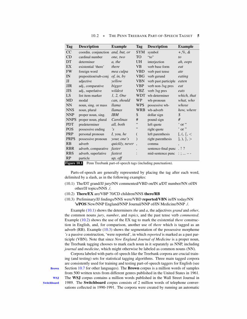
10.2 • THE PENN TREEBANK PART-OF-SPEECH TAGSET 5

Tag Description Example Tag Description ExampleCC coordin. conjunction and, but, or SYM symbol +,%, &CD cardinal number one, two TO “to” toDT determiner a, the UH interjection ah, oopsEX existential ‘there’ there VB verb base form eatFW foreign word mea culpa VBD verb past tense ateIN preposition/sub-conj of, in, by VBG verb gerund eatingJJ adjective yellow VBN verb past participle eatenJJR adj., comparative bigger VBP verb non-3sg pres eatJJS adj., superlative wildest VBZ verb 3sg pres eatsLS list item marker 1, 2, One WDT wh-determiner which, thatMD modal can, should WP wh-pronoun what, whoNN noun, sing. or mass llama WP$ possessive wh- whoseNNS noun, plural llamas WRB wh-adverb how, whereNNP proper noun, sing. IBM $ dollar sign $NNPS proper noun, plural Carolinas # pound sign #PDT predeterminer all, both “ left quote ‘ or “POS possessive ending ’s ” right quote ’ or ”PRP personal pronoun I, you, he ( left parenthesis [, (, {, <PRP$ possessive pronoun your, one’s ) right parenthesis ], ), }, >RB adverb quickly, never , comma ,RBR adverb, comparative faster . sentence-final punc . ! ?RBS adverb, superlative fastest : mid-sentence punc : ; ... – -RP particle up, off

Figure 10.1 Penn Treebank part-of-speech tags (including punctuation).

Parts-of-speech are generally represented by placing the tag after each word,delimited by a slash, as in the following examples:

(10.1) The/DT grand/JJ jury/NN commented/VBD on/IN a/DT number/NN of/INother/JJ topics/NNS ./.

(10.2) There/EX are/VBP 70/CD children/NNS there/RB(10.3) Preliminary/JJ findings/NNS were/VBD reported/VBN in/IN today/NN

’s/POS New/NNP England/NNP Journal/NNP of/IN Medicine/NNP ./.

Example (10.1) shows the determiners the and a, the adjectives grand and other,the common nouns jury, number, and topics, and the past tense verb commented.Example (10.2) shows the use of the EX tag to mark the existential there construc-tion in English, and, for comparison, another use of there which is tagged as anadverb (RB). Example (10.3) shows the segmentation of the possessive morpheme’s a passive construction, ‘were reported’, in which reported is marked as a past par-ticiple (VBN). Note that since New England Journal of Medicine is a proper noun,the Treebank tagging chooses to mark each noun in it separately as NNP, includingjournal and medicine, which might otherwise be labeled as common nouns (NN).

Corpora labeled with parts-of-speech like the Treebank corpora are crucial train-ing (and testing) sets for statistical tagging algorithms. Three main tagged corporaare consistently used for training and testing part-of-speech taggers for English (seeSection 10.7 for other languages). The Brown corpus is a million words of samplesBrown

from 500 written texts from different genres published in the United States in 1961.The WSJ corpus contains a million words published in the Wall Street Journal inWSJ

1989. The Switchboard corpus consists of 2 million words of telephone conver-Switchboard

sations collected in 1990-1991. The corpora were created by running an automatic


part-of-speech tagger on the texts and then human annotators hand-corrected eachtag.

There are some minor differences in the tagsets used by the corpora. For examplein the WSJ and Brown corpora, the single Penn tag TO is used for both the infinitiveto (I like to race) and the preposition to (go to the store), while in the Switchboardcorpus the tag TO is reserved for the infinitive use of to, while the preposition use istagged IN:

Well/UH ,/, I/PRP ,/, I/PRP want/VBP to/TO go/VB to/IN a/DT restaurant/NN

Finally, there are some idiosyncracies inherent in any tagset. For example, be-cause the Penn 45 tags were collapsed from a larger 87-tag tagset, the originalBrown tagset, some potential useful distinctions were lost. The Penn tagset wasdesigned for a treebank in which sentences were parsed, and so it leaves off syntac-tic information recoverable from the parse tree. Thus for example the Penn tag IN isused for both subordinating conjunctions like if, when, unless, after:

after/IN spending/VBG a/DT day/NN at/IN the/DT beach/NN

and prepositions like in, on, after:

after/IN sunrise/NN

Tagging algorithms assume that words have been tokenized before tagging. ThePenn Treebank and the British National Corpus split contractions and the ’s-genitivefrom their stems:

would/MD n’t/RBchildren/NNS ’s/POS

Indeed, the special Treebank tag POS is used only for the morpheme ’s, whichmust be segmented off during tokenization.

Another tokenization issue concerns multipart words. The Treebank tagset as-sumes that tokenization of words like New York is done at whitespace. The phrasea New York City firm is tagged in Treebank notation as five separate words: a/DTNew/NNP York/NNP City/NNP firm/NN. The C5 tagset for the British National Cor-pus, by contrast, allow prepositions like “in terms of” to be treated as a single wordby adding numbers to each tag, as in in/II31 terms/II32 of/II33.

10.3 Part-of-Speech Tagging

Part-of-speech tagging (tagging for short) is the process of assigning a part-of-tagging

speech marker to each word in an input text. Because tags are generally also appliedto punctuation, tokenization is usually performed before, or as part of, the taggingprocess: separating commas, quotation marks, etc., from words and disambiguatingend-of-sentence punctuation (period, question mark, etc.) from part-of-word punc-tuation (such as in abbreviations like e.g. and etc.)

The input to a tagging algorithm is a sequence of words and a tagset, and theoutput is a sequence of tags, a single best tag for each word as shown in the exampleson the previous pages.

Tagging is a disambiguation task; words are ambiguous —have more than oneambiguous

possible part-of-speech— and the goal is to find the correct tag for the situation. Forexample, the word book can be a verb (book that flight) or a noun (as in hand methat book.

10.3 • PART-OF-SPEECH TAGGING 7

That can be a determiner (Does that flight serve dinner) or a complementizer(I thought that your flight was earlier). The problem of POS-tagging is to resolveresolution

these ambiguities, choosing the proper tag for the context. Part-of-speech tagging isthus one of the many disambiguation tasks in language processing.disambiguation

How hard is the tagging problem? And how common is tag ambiguity? Fig. 10.2shows the answer for the Brown and WSJ corpora tagged using the 45-tag Penntagset. Most word types (80-86%) are unambiguous; that is, they have only a sin-gle tag (Janet is always NNP, funniest JJS, and hesitantly RB). But the ambiguouswords, although accounting for only 14-15% of the vocabulary, are some of themost common words of English, and hence 55-67% of word tokens in running textare ambiguous. Note the large differences across the two genres, especially in tokenfrequency. Tags in the WSJ corpus are less ambiguous, presumably because thisnewspaper’s specific focus on financial news leads to a more limited distribution ofword usages than the more general texts combined into the Brown corpus.

Types: WSJ BrownUnambiguous (1 tag) 44,432 (86%) 45,799 (85%)Ambiguous (2+ tags) 7,025 (14%) 8,050 (15%)

Tokens:Unambiguous (1 tag) 577,421 (45%) 384,349 (33%)Ambiguous (2+ tags) 711,780 (55%) 786,646 (67%)

Figure 10.2 The amount of tag ambiguity for word types in the Brown and WSJ corpora,from the Treebank-3 (45-tag) tagging. These statistics include punctuation as words, andassume words are kept in their original case.

Some of the most ambiguous frequent words are that, back, down, put and set;here are some examples of the 6 different parts-of-speech for the word back:

earnings growth took a back/JJ seata small building in the back/NNa clear majority of senators back/VBP the billDave began to back/VB toward the doorenable the country to buy back/RP about debtI was twenty-one back/RB then

Still, even many of the ambiguous tokens are easy to disambiguate. This isbecause the different tags associated with a word are not equally likely. For ex-ample, a can be a determiner or the letter a (perhaps as part of an acronym or aninitial). But the determiner sense of a is much more likely. This idea suggests asimplistic baseline algorithm for part of speech tagging: given an ambiguous word,choose the tag which is most frequent in the training corpus. This is a key concept:

Most Frequent Class Baseline: Always compare a classifier against a baseline atleast as good as the most frequent class baseline (assigning each token to the classit occurred in most often in the training set).

How good is this baseline? A standard way to measure the performance of part-of-speech taggers is accuracy: the percentage of tags correctly labeled on a human-accuracy

labeled test set. One commonly used test set is sections 22-24 of the WSJ corpus. Ifwe train on the rest of the WSJ corpus and test on that test set, the most-frequent-tagbaseline achieves an accuracy of 92.34%.

By contrast, the state of the art in part-of-speech tagging on this dataset is around97% tag accuracy, a performance that is achievable by a number of statistical algo-


rithms including HMMs, MEMMs and other log-linear models, perceptrons, andprobably also rule-based systems—see the discussion at the end of the chapter. SeeSection 10.7 on other languages and genres.

10.4 HMM Part-of-Speech Tagging

In this section we introduce the use of the Hidden Markov Model for part-of-speechtagging. The HMM defined in the previous chapter was quite powerful, including alearning algorithm— the Baum-Welch (EM) algorithm—that can be given unlabeleddata and find the best mapping of labels to observations. However when we applyHMM to part-of-speech tagging we generally don’t use the Baum-Welch algorithmfor learning the HMM parameters. Instead HMMs for part-of-speech tagging aretrained on a fully labeled dataset—a set of sentences with each word annotated witha part-of-speech tag—setting parameters by maximum likelihood estimates on thistraining data.

Thus the only algorithm we will need from the previous chapter is the Viterbialgorithm for decoding, and we will also need to see how to set the parameters fromtraining data.

10.4.1 The basic equation of HMM TaggingLet’s begin with a quick reminder of the intuition of HMM decoding. The goalof HMM decoding is to choose the tag sequence that is most probable given theobservation sequence of n words wn

1:

tn1 = argmax

tn1

P(tn1 |wn

1) (10.4)

by using Bayes’ rule to instead compute:

tn1 = argmax

tn1

P(wn1|tn

1 )P(tn1 )

P(wn1)

(10.5)

Furthermore, we simplify Eq. 10.5 by dropping the denominator P(wn1):

tn1 = argmax

tn1

P(wn1|tn

1 )P(tn1 ) (10.6)

HMM taggers make two further simplifying assumptions. The first is that theprobability of a word appearing depends only on its own tag and is independent ofneighboring words and tags:

P(wn1|tn

1 ) ≈n∏

i=1

P(wi|ti) (10.7)

The second assumption, the bigram assumption, is that the probability of a tagis dependent only on the previous tag, rather than the entire tag sequence;

P(tn1 ) ≈

n∏i=1

P(ti|ti−1) (10.8)

10.4 • HMM PART-OF-SPEECH TAGGING 9

Plugging the simplifying assumptions from Eq. 10.7 and Eq. 10.8 into Eq. 10.6results in the following equation for the most probable tag sequence from a bigramtagger, which as we will soon see, correspond to the emission probability and tran-sition probability from the HMM of Chapter 9.

tn1 = argmax

tn1

P(tn1 |wn

1)≈ argmaxtn1

n∏i=1

emission︷︸︸︷P(wi|ti)

transition︷︸︸︷P(ti|ti−1) (10.9)

10.4.2 Estimating probabilitiesLet’s walk through an example, seeing how these probabilities are estimated andused in a sample tagging task, before we return to the Viterbi algorithm.

In HMM tagging, rather than using the full power of HMM EM learning, theprobabilities are estimated just by counting on a tagged training corpus. For thisexample we’ll use the tagged WSJ corpus. The tag transition probabilities P(ti|ti−1)represent the probability of a tag given the previous tag. For example, modal verbslike will are very likely to be followed by a verb in the base form, a VB, like race,so we expect this probability to be high. The maximum likelihood estimate of atransition probability is computed by counting, out of the times we see the first tagin a labeled corpus, how often the first tag is followed by the second

P(ti|ti−1) =C(ti−1, ti)C(ti−1)

(10.10)

In the WSJ corpus, for example, MD occurs 13124 times of which it is followedby VB 10471, for an MLE estimate of

P(V B|MD) =C(MD,V B)

C(MD)=

1047113124

= .80 (10.11)

The emission probabilities, P(wi|ti), represent the probability, given a tag (sayMD), that it will be associated with a given word (say will). The MLE of the emis-sion probability is

P(wi|ti) =C(ti,wi)

C(ti)(10.12)

Of the 13124 occurrences of MD in the WSJ corpus, it is associated with will 4046times:

P(will|MD) =C(MD,will)

C(MD)=

404613124

= .31 (10.13)

For those readers who are new to Bayesian modeling, note that this likelihoodterm is not asking “which is the most likely tag for the word will?” That would bethe posterior P(MD|will). Instead, P(will|MD) answers the slightly counterintuitivequestion “If we were going to generate a MD, how likely is it that this modal wouldbe will?”

The two kinds of probabilities from Eq. 10.9, the transition (prior) probabilitieslike P(V B|MD) and the emission (likelihood) probabilities like P(will|MD), corre-spond to the A transition probabilities, and B observation likelihoods of the HMM.Figure 10.3 illustrates some of the the A transition probabilities for three states in anHMM part-of-speech tagger; the full tagger would have one state for each tag.

Figure 10.4 shows another view of these three states from an HMM tagger, fo-cusing on the word likelihoods B. Each hidden state is associated with a vector oflikelihoods for each observation word.


Start0 End4

NN3VB1

MD2

a22

a02

a11

a12

a03

a01

a21

a13

a33

a24

a14

a32

a23

a31

a34

Figure 10.3 A piece of the Markov chain corresponding to the hidden states of the HMM.The A transition probabilities are used to compute the prior probability.

Start0 End4

NN3VB1

MD2

P("aardvark" | NN)...P(“will” | NN)...P("the" | NN)...P(“back” | NN)...P("zebra" | NN)

P("aardvark" | VB)...P(“will” | VB)...P("the" | VB)...P(“back” | VB)...P("zebra" | VB)

P("aardvark" | MD)...P(“will” | MD)...P("the" | MD)...P(“back” | MD)...P("zebra" | MD)

B3B1

B2

Figure 10.4 Some of the B observation likelihoods for the HMM in the previous figure.Each state (except the non-emitting start and end states) is associated with a vector of proba-bilities, one likelihood for each possible observation word.

10.4.3 Working through an exampleLet’s now work through an example of computing the best sequence of tags thatcorresponds to the following sequence of words

(10.14) Janet will back the bill

The correct series of tags is:

(10.15) Janet/NNP will/MD back/VB the/DT bill/NN

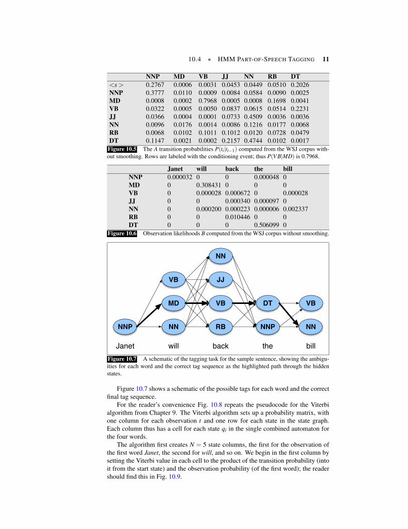
Let the HMM be defined by the two tables in Fig. 10.5 and Fig. 10.6.Figure 10.5 lists the ai j probabilities for transitioning between the hidden states

(part-of-speech tags).Figure 10.6 expresses the bi(ot) probabilities, the observation likelihoods of

words given tags. This table is (slightly simplified) from counts in the WSJ cor-pus. So the word Janet only appears as an NNP, back has 4 possible parts of speech,and the word the can appear as a determiner or as an NNP (in titles like “SomewhereOver the Rainbow” all words are tagged as NNP).


NNP MD VB JJ NN RB DT<s > 0.2767 0.0006 0.0031 0.0453 0.0449 0.0510 0.2026NNP 0.3777 0.0110 0.0009 0.0084 0.0584 0.0090 0.0025MD 0.0008 0.0002 0.7968 0.0005 0.0008 0.1698 0.0041VB 0.0322 0.0005 0.0050 0.0837 0.0615 0.0514 0.2231JJ 0.0366 0.0004 0.0001 0.0733 0.4509 0.0036 0.0036NN 0.0096 0.0176 0.0014 0.0086 0.1216 0.0177 0.0068RB 0.0068 0.0102 0.1011 0.1012 0.0120 0.0728 0.0479DT 0.1147 0.0021 0.0002 0.2157 0.4744 0.0102 0.0017

Figure 10.5 The A transition probabilities P(ti|ti−1) computed from the WSJ corpus with-out smoothing. Rows are labeled with the conditioning event; thus P(V B|MD) is 0.7968.

Janet will back the billNNP 0.000032 0 0 0.000048 0MD 0 0.308431 0 0 0VB 0 0.000028 0.000672 0 0.000028JJ 0 0 0.000340 0.000097 0NN 0 0.000200 0.000223 0.000006 0.002337RB 0 0 0.010446 0 0DT 0 0 0 0.506099 0

Figure 10.6 Observation likelihoods B computed from the WSJ corpus without smoothing.

NNP

Janet will back the bill

NN

MD

VB

RB

VB

JJ

NN

NNP

DT

NN

VB

Figure 10.7 A schematic of the tagging task for the sample sentence, showing the ambigu-ities for each word and the correct tag sequence as the highlighted path through the hiddenstates.

Figure 10.7 shows a schematic of the possible tags for each word and the correctfinal tag sequence.

For the reader’s convenience Fig. 10.8 repeats the pseudocode for the Viterbialgorithm from Chapter 9. The Viterbi algorithm sets up a probability matrix, withone column for each observation t and one row for each state in the state graph.Each column thus has a cell for each state qi in the single combined automaton forthe four words.

The algorithm first creates N = 5 state columns, the first for the observation ofthe first word Janet, the second for will, and so on. We begin in the first column bysetting the Viterbi value in each cell to the product of the transition probability (intoit from the start state) and the observation probability (of the first word); the readershould find this in Fig. 10.9.


function VITERBI(observations of len T,state-graph of len N) returns best-path

create a path probability matrix viterbi[N+2,T]for each state s from 1 to N do ; initialization step

viterbi[s,1]←a0,s ∗ bs(o1)backpointer[s,1]←0

for each time step t from 2 to T do ; recursion stepfor each state s from 1 to N do

viterbi[s,t]← Nmax

s′=1viterbi[s′, t−1] ∗ as′,s ∗ bs(ot)

backpointer[s,t]← Nargmax

s′=1

viterbi[s′, t−1] ∗ as′,s

viterbi[qF ,T]← Nmax

s=1viterbi[s,T ] ∗ as,qF ; termination step

backpointer[qF ,T]← Nargmax

s=1

viterbi[s,T ] ∗ as,qF ; termination step

return the backtrace path by following backpointers to states back in time frombackpointer[qF ,T ]

Figure 10.8 Viterbi algorithm for finding optimal sequence of tags. Given an observationsequence and an HMM λ = (A,B), the algorithm returns the state path through the HMMthat assigns maximum likelihood to the observation sequence. Note that states 0 and qF arenon-emitting.

Then we move on, column by column; for every state in column 1, we computethe probability of moving into each state in column 2, and so on. For each state q j attime t, we compute the value viterbi[s, t] by taking the maximum over the extensionsof all the paths that lead to the current cell, using the following equation:

vt( j) =N

maxi=1

vt−1(i) ai j b j(ot) (10.16)

Recall from Chapter 9 that the three factors that are multiplied in Eq. 10.16 forextending the previous paths to compute the Viterbi probability at time t are

vt−1(i) the previous Viterbi path probability from the previous time stepai j the transition probability from previous state qi to current state q j

b j(ot) the state observation likelihood of the observation symbol ot giventhe current state j

In Fig. 10.9, each cell of the trellis in the column for the word Janet is com-puted by multiplying the previous probability at the start state (1.0), the transitionprobability from the start state to the tag for that cell, and the observation likelihoodof the word Janet given the tag for that cell. Most of the cells in the column arezero since the word Janet cannot be any of those tags. Next, each cell in the willcolumn gets updated with the maximum probability path from the previous column.We have shown the values for the MD, VB, and NN cells. Each cell gets the maxof the 7 values from the previous column, multiplied by the appropriate transitionprobability; as it happens in this case, most of them are zero from the previous col-umn. The remaining value is multiplied by the relevant transition probability, andthe (trivial) max is taken. In this case the final value, .0000002772, comes from theNNP state at the previous column. The reader should fill in the rest of the trellis inFig. 10.9 and backtrace to reconstruct the correct state sequence NNP MD VB DTNN. (Exercise 10.??).


start

P(NNP|start)

= .28

* P(MD|MD)= 0

* P(M

D|NNP)

.0000

09*.0

1 = .

0000

009

P(MD|start)

= .0006v1(2)=

.0006 x 0 = 0

v1(1) = .28* .000032

= .000009

t

MD

end endqend

q2

q1

q0

o1

Janet billwillo2 o3

end

back

VB

JJ

v1(3)=.0031 x 0

= 0

v1(4)= .045*0=0

o4

* P(MD|VB) = 0

* P(MD|JJ)

= 0

v0(0) = 1.0

P(VB|start)

= .0031

P(JJ |st

art) =

.045

backtrace

backtrace

q3

q4

end

the

NNq5

RBq6

DTq7

endend

v2(2) =max * .308 =.0000002772

v2(5)=max * .0002 = .0000000001

v2(3)=max * .000028

= 2.5e-11

v3(6)=max * .0104

v3(5)=max * .000223

v3(4)=max * .00034

v3(3)=max * .00067

v1(5)

v1(6)

v1(7)

v2(1)

v2(4)

v2(6)

v2(7)

backtrace

* P(R

B|NN)

* P(NN|NN)

start start start start start

o5

NNP

Figure 10.9 The first few entries in the individual state columns for the Viterbi algorithm. Each cell keepsthe probability of the best path so far and a pointer to the previous cell along that path. We have only filled outcolumns 1 and 2; to avoid clutter most cells with value 0 are left empty. The rest is left as an exercise for thereader. After the cells are filled in, backtracing from the end state, we should be able to reconstruct the correctstate sequence NNP MD VB DT NN.

10.4.4 Extending the HMM Algorithm to TrigramsPractical HMM taggers have a number of extensions of this simple model. Oneimportant missing feature is a wider tag context. In the tagger described above theprobability of a tag depends only on the previous tag:

P(tn1 ) ≈

n∏i=1

P(ti|ti−1) (10.17)

In practice we use more of the history, letting the probability of a tag depend onthe two previous tags:

P(tn1 ) ≈

n∏i=1

P(ti|ti−1, ti−2) (10.18)

Extending the algorithm from bigram to trigram taggers gives a small (perhaps ahalf point) increase in performance, but conditioning on two previous tags instead ofone requires a significant change to the Viterbi algorithm. For each cell, instead oftaking a max over transitions from each cell in the previous column, we have to take


a max over paths through the cells in the previous two columns, thus considering N2

rather than N hidden states at every observation.In addition to increasing the context window, state-of-the-art HMM taggers like

Brants (2000) have a number of other advanced features. One is to let the taggerknow the location of the end of the sentence by adding dependence on an end-of-sequence marker for tn+1. This gives the following equation for part-of-speech tag-ging:

tn1 = argmax

tn1

P(tn1 |wn

1)≈ argmaxtn1

[n∏

i=1

P(wi|ti)P(ti|ti−1, ti−2)

]P(tn+1|tn) (10.19)

In tagging any sentence with Eq. 10.19, three of the tags used in the context willfall off the edge of the sentence, and hence will not match regular words. These tags,t−1, t0, and tn+1, can all be set to be a single special ‘sentence boundary’ tag that isadded to the tagset, which assumes sentences boundaries have already been marked.

One problem with trigram taggers as instantiated in Eq. 10.19 is data sparsity.Any particular sequence of tags ti−2, ti−1, ti that occurs in the test set may simplynever have occurred in the training set. That means we cannot compute the tagtrigram probability just by the maximum likelihood estimate from counts, followingEq. 10.20:

P(ti|ti−1, ti−2) =C(ti−2, ti−1, ti)C(ti−2, ti−1)

(10.20)

Just as we saw with language modeling, many of these counts will be zeroin any training set, and we will incorrectly predict that a given tag sequence willnever occur! What we need is a way to estimate P(ti|ti−1, ti−2) even if the sequenceti−2, ti−1, ti never occurs in the training data.

The standard approach to solving this problem is the same interpolation ideawe saw in language modeling: estimate the probability by combining more robust,but weaker estimators. For example, if we’ve never seen the tag sequence PRP VBTO, and so can’t compute P(TO|PRP,VB) from this frequency, we still could relyon the bigram probability P(TO|VB), or even the unigram probability P(TO). Themaximum likelihood estimation of each of these probabilities can be computed froma corpus with the following counts:

Trigrams P(ti|ti−1, ti−2) =C(ti−2, ti−1, ti)C(ti−2, ti−1)

(10.21)

Bigrams P(ti|ti−1) =C(ti−1, ti)C(ti−1)

(10.22)

Unigrams P(ti) =C(ti)

N(10.23)

The standard way to combine these three estimators to estimate the trigramprobability P(ti|ti−1, ti−2)? is via linear interpolation. We estimate the probabilityP(ti|ti−1ti−2) by a weighted sum of the unigram, bigram, and trigram probabilities:

P(ti|ti−1ti−2) = λ3P(ti|ti−1ti−2)+λ2P(ti|ti−1)+λ1P(ti) (10.24)

We require λ1 +λ2 +λ3 = 1, ensuring that the resulting P is a probability dis-tribution. These λ s are generally set by an algorithm called deleted interpolationdeleted

interpolation


(Jelinek and Mercer, 1980): we successively delete each trigram from the trainingcorpus and choose the λ s so as to maximize the likelihood of the rest of the corpus.The deletion helps to set the λ s in such a way as to generalize to unseen data andnot overfit the training corpus. Figure 10.10 gives a deleted interpolation algorithmfor tag trigrams.

function DELETED-INTERPOLATION(corpus) returns λ1,λ2,λ3

λ1←0λ2←0λ3←0foreach trigram t1, t2, t3 with C(t1, t2, t3)> 0

depending on the maximum of the following three valuescase C(t1,t2,t3)−1

C(t1,t2)−1 : increment λ3 by C(t1, t2, t3)

case C(t2,t3)−1C(t2)−1 : increment λ2 by C(t1, t2, t3)

case C(t3)−1N−1 : increment λ1 by C(t1, t2, t3)

endendnormalize λ1,λ2,λ3return λ1,λ2,λ3

Figure 10.10 The deleted interpolation algorithm for setting the weights for combiningunigram, bigram, and trigram tag probabilities. If the denominator is 0 for any case, wedefine the result of that case to be 0. N is the total number of tokens in the corpus. AfterBrants (2000).

10.4.5 Unknown Wordswords peoplenever use —could beonly Iknow them

Ishikawa Takuboku 1885–1912

To achieve high accuracy with part-of-speech taggers, it is also important to havea good model for dealing with unknown words. Proper names and acronyms areunknown

wordscreated very often, and even new common nouns and verbs enter the language at asurprising rate. One useful feature for distinguishing parts of speech is wordshape:words starting with capital letters are likely to be proper nouns (NNP).

But the strongest source of information for guessing the part-of-speech of un-known words is morphology. Words that end in -s are likely to be plural nouns(NNS), words ending with -ed tend to be past participles (VBN), words ending with-able tend to be adjectives (JJ), and so on. One way to take advantage of this isto store for each final letter sequence (for simplicity referred to as word suffixes)the statistics of which tag they were associated with in training. The method ofSamuelsson (1993) and Brants (2000), for example, considers suffixes of up to tenletters, computing for each suffix of length i the probability of the tag ti given thesuffix letters:

P(ti|ln−i+1 . . . ln) (10.25)


They use back-off to smooth these probabilities with successively shorter andshorter suffixes. To capture the fact that unknown words are unlikely to be closed-class words like prepositions, we can compute suffix probabilities only from thetraining set for words whose frequency in the training set is ≤ 10, or alternately cantrain suffix probabilities only on open-class words. Separate suffix tries are kept forcapitalized and uncapitalized words.

Finally, because Eq. 10.25 gives a posterior estimate p(ti|wi), we can computethe likelihood p(wi|ti) that HMMs require by using Bayesian inversion (i.e., usingBayes rule and computation of the two priors P(ti) and P(ti|ln−i+1 . . . ln)).

In addition to using capitalization information for unknown words, Brants (2000)also uses capitalization for known words by adding a capitalization feature to eachtag. Thus, instead of computing P(ti|ti−1, ti−2) as in Eq. 10.21, the algorithm com-putes the probability P(ti,ci|ti−1,ci−1, ti−2,ci−2). This is equivalent to having a cap-italized and uncapitalized version of each tag, essentially doubling the size of thetagset.

Combining all these features, a state-of-the-art trigram HMM like that of Brants(2000) has a tagging accuracy of 96.7% on the Penn Treebank.

10.5 Maximum Entropy Markov Models

We turn now to a second sequence model, the maximum entropy Markov modelor MEMM. The MEMM is a sequence model adaptation of the MaxEnt (multino-MEMM

mial logistic regression) classifier. Because it is based on logistic regression, theMEMM is a discriminative sequence model. By contrast, the HMM is a genera-discriminative

tive sequence model.generative

Let the sequence of words be W = wn1 and the sequence of tags T = tn

1 . In anHMM to compute the best tag sequence that maximizes P(T |W ) we rely on Bayes’rule and the likelihood P(W |T ):

T = argmaxT

P(T |W )

= argmaxT

P(W |T )P(T )

= argmaxT

∏i

P(wordi|tagi)∏

i

P(tagi|tagi−1) (10.26)

In an MEMM, by contrast, we compute the posterior P(T |W ) directly, trainingit to discriminate among the possible tag sequences:

T = argmaxT

P(T |W )

= argmaxT

∏i

P(ti|wi, ti−1) (10.27)

We could do this by training a logistic regression classifier to compute the singleprobability P(ti|wi, ti−1). Fig. 10.11 shows the intuition of the difference via thedirection of the arrows; HMMs compute likelihood (observation word conditionedon tags) but MEMMs compute posterior (tags conditioned on observation words).

10.5 • MAXIMUM ENTROPY MARKOV MODELS 17

will

MD VB DT NN

Janet back the bill

NNP

will

MD VB DT NN

Janet back the bill

NNP

Figure 10.11 A schematic view of the HMM (top) and MEMM (bottom) representation ofthe probability computation for the correct sequence of tags for the back sentence. The HMMcomputes the likelihood of the observation given the hidden state, while the MEMM computesthe posterior of each state, conditioned on the previous state and current observation.

10.5.1 Features in a MEMMOops. We lied in Eq. 10.27. We actually don’t build MEMMs that condition just onwi and ti−1. In fact, an MEMM conditioned on just these two features (the observedword and the previous tag), as shown in Fig. 10.11 and Eq. 10.27 is no more accuratethan the generative HMM model and in fact may be less accurate.

The reason to use a discriminative sequence model is that discriminative modelsmake it easier to incorporate a much wider variety of features. Because in HMMsall computation is based on the two probabilities P(tag|tag) and P(word|tag), if wewant to include some source of knowledge into the tagging process, we must finda way to encode the knowledge into one of these two probabilities. We saw in theprevious section that it was possible to model capitalization or word endings bycleverly fitting in probabilities like P(capitalization|tag), P(suffix|tag), and so oninto an HMM-style model. But each time we add a feature we have to do a lot ofcomplicated conditioning which gets harder and harder as we have more and moresuch features and, as we’ll see, there are lots more features we can add. Figure 10.12shows a graphical intuition of some of these additional features.

will

MD VB

Janet back the bill

NNP

<s>

wi wi+1wi-1

ti-1ti-2

wi-1

Figure 10.12 An MEMM for part-of-speech tagging showing the ability to condition onmore features.

A basic MEMM part-of-speech tagger conditions on the observation word it-self, neighboring words, and previous tags, and various combinations, using featuretemplates like the following:templates

〈ti,wi−2〉,〈ti,wi−1〉,〈ti,wi〉,〈ti,wi+1〉,〈ti,wi+2〉〈ti, ti−1〉,〈ti, ti−2, ti−1〉,

〈ti, ti−1,wi〉,〈ti,wi−1,wi〉〈ti,wi,wi+1〉, (10.28)


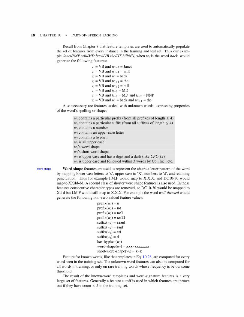
Recall from Chapter 8 that feature templates are used to automatically populatethe set of features from every instance in the training and test set. Thus our exam-ple Janet/NNP will/MD back/VB the/DT bill/NN, when wi is the word back, wouldgenerate the following features:

ti = VB and wi−2 = Janetti = VB and wi−1 = willti = VB and wi = backti = VB and wi+1 = theti = VB and wi+2 = billti = VB and ti−1 = MDti = VB and ti−1 = MD and ti−2 = NNPti = VB and wi = back and wi+1 = the

Also necessary are features to deal with unknown words, expressing propertiesof the word’s spelling or shape:

wi contains a particular prefix (from all prefixes of length ≤ 4)wi contains a particular suffix (from all suffixes of length ≤ 4)wi contains a numberwi contains an upper-case letterwi contains a hyphenwi is all upper casewi’s word shapewi’s short word shapewi is upper case and has a digit and a dash (like CFC-12)wi is upper case and followed within 3 words by Co., Inc., etc.

Word shape features are used to represent the abstract letter pattern of the wordword shape

by mapping lower-case letters to ‘x’, upper-case to ‘X’, numbers to ’d’, and retainingpunctuation. Thus for example I.M.F would map to X.X.X. and DC10-30 wouldmap to XXdd-dd. A second class of shorter word shape features is also used. In thesefeatures consecutive character types are removed, so DC10-30 would be mapped toXd-d but I.M.F would still map to X.X.X. For example the word well-dressed wouldgenerate the following non-zero valued feature values:

prefix(wi) = wprefix(wi) = weprefix(wi) = welprefix(wi) = wellsuffix(wi) = ssedsuffix(wi) = sedsuffix(wi) = edsuffix(wi) = dhas-hyphen(wi)word-shape(wi) = xxx-xxxxxxxshort-word-shape(wi) = x-x

Feature for known words, like the templates in Eq. 10.28, are computed for everyword seen in the training set. The unknown word features can also be computed forall words in training, or only on rare training words whose frequency is below somethreshold.

The result of the known-word templates and word-signature features is a verylarge set of features. Generally a feature cutoff is used in which features are thrownout if they have count < 5 in the training set.

10.5 • MAXIMUM ENTROPY MARKOV MODELS 19

Given this large set of features, the most likely sequence of tags is then computedby a MaxEnt model that combines these features of the input word wi, its neighborswithin l words wi+l

i−l , and the previous k tags t i−1i−k as follows:

T = argmaxT

P(T |W )

= argmaxT

∏i

P(ti|wi+li−l , t

i−1i−k )

= argmaxT

∏i

exp

(∑i

wi fi(ti,wi+li−l , t

i−1i−k )

)∑

t ′∈tagsetexp

(∑i

wi fi(t ′,wi+li−l , t

i−1i−k )

) (10.29)

10.5.2 Decoding and Training MEMMsWe’re now ready to see how to use the MaxEnt classifier to solve the decodingproblem by finding the most likely sequence of tags described in Eq. 10.29.

The simplest way to turn the MaxEnt classifier into a sequence model is to builda local classifier that classifies each word left to right, making a hard classificationof the first word in the sentence, then a hard decision on the the second word, andso on. This is called a greedy decoding algorithm, because we greedily choose thegreedy

best tag for each word, as shown in Fig. 10.13.

function GREEDY MEMM DECODING(words W, model P) returns tag sequence T

for i = 1 to length(W)ti = argmax

t ′∈ TP(t ′ | wi+l

i−l , ti−1i−k )

Figure 10.13 In greedy decoding we make a hard decision to choose the best tag left toright.

The problem with the greedy algorithm is that by making a hard decision on eachword before moving on to the next word, the classifier cannot temper its decisionwith information from future decisions. Although greedy algorithm is very fast, andwe do use it in some applications when it has sufficient accuracy, in general this harddecision causes sufficient drop in performance that we don’t use it.

Instead we decode an MEMM with the Viterbi algorithm just as we did with theViterbi

HMM, thus finding the sequence of part-of-speech tags that is optimal for the wholesentence.

Let’s see an example. For pedagogical purposes, let’s assume for this examplethat our MEMM is only conditioning on the previous tag ti−1 and observed wordwi. Concretely, this involves filling an N×T array with the appropriate values forP(ti|ti−1,wi), maintaining backpointers as we proceed. As with HMM Viterbi, whenthe table is filled, we simply follow pointers back from the maximum value in thefinal column to retrieve the desired set of labels. The requisite changes from theHMM-style application of Viterbi have to do only with how we fill each cell. Recallfrom Eq. ?? that the recursive step of the Viterbi equation computes the Viterbi valueof time t for state j as


vt( j) =N

maxi=1

vt−1(i)ai j b j(ot); 1≤ j ≤ N,1 < t ≤ T (10.30)

which is the HMM implementation of

vt( j) =N

maxi=1

vt−1(i) P(s j|si) P(ot |s j) 1≤ j ≤ N,1 < t ≤ T (10.31)

The MEMM requires only a slight change to this latter formula, replacing the aand b prior and likelihood probabilities with the direct posterior:

vt( j) =N

maxi=1

vt−1(i) P(s j|si,ot) 1≤ j ≤ N,1 < t ≤ T (10.32)

Figure 10.14 shows an example of the Viterbi trellis for an MEMM applied tothe ice-cream task from Section ??. Recall that the task is figuring out the hiddenweather (hot or cold) from observed numbers of ice creams eaten in Jason Eisner’sdiary. Figure 10.14 shows the abstract Viterbi probability calculation, assuming thatwe have a MaxEnt model that computes P(si|si−1,oi) for us.

start

H

C

H

C

H

C

end

P(C|start,3

)

P(H|H,1)

P(C|C,1)

P(C|H,1)

P(H|C,1)

P(H|

start,

3)

v1(2)=P(H|start,3)

v1(1) = P(C|start,3)

v2(2)= max( P(H|H,1)*P(H|start,3), P(H|C,1)*P(C|start,3) )

v2(1) = max( P(C|H,1)*P(H|start,3), P(C|C,1)*P(C|start,3) )

start start start

t

C

H

end end end end

H

C

start

qend

q2

q1

q0

o1 o2 o3

3 1 1

Figure 10.14 Inference from ice-cream eating computed by an MEMM instead of an HMM. The Viterbitrellis for computing the best path through the hidden state space for the ice-cream eating events 3 1 3, modifiedfrom the HMM figure in Fig. ??.

Learning in MEMMs relies on the same supervised learning algorithms we pre-sented for logistic regression. Given a sequence of observations, feature functions,and corresponding hidden states, we train the weights so as maximize the log-likelihood of the training corpus. As with logistic regression, regularization is im-portant, and all modern systems use L1 or L2 regularization.

10.6 • BIDIRECTIONALITY 21

10.6 Bidirectionality

The one problem with the MEMM and HMM models as presented is that they areexclusively run left-to-right. While the Viterbi algorithm still allows present deci-sions to be influenced indirectly by future decisions, it would help even more if adecision about word wi could directly use information about future tags ti+1 and ti+2.

Adding bidirectionality has another useful advantage. MEMMs have a theoret-ical weakness, referred to alternatively as the label bias or observation bias prob-label bias

observationbias lem (Lafferty et al. 2001, Toutanova et al. 2003). These are names for situations

when one source of information is ignored because it is explained away by anothersource. Consider an example from (Toutanova et al., 2003), the sequence will/NNto/TO fight/VB. The tag TO is often preceded by NN but rarely by modals (MD),and so that tendency should help predict the correct NN tag for will. But the previ-ous transition P(twill |〈s〉) prefers the modal, and because P(TO|to, twill) is so closeto 1 regardless of twill the model cannot make use of the transition probability andincorrectly chooses MD. The strong information that to must have the tag TO has ex-plained away the presence of TO and so the model doesn’t learn the importance ofthe previous NN tag for predicting TO. Bidirectionality helps the model by makingthe link between TO available when tagging the NN.

One way to implement bidirectionality is to switch to a much more powerfulmodel called a Conditional Random Field or CRF, which we will introduce inCRF

Chapter 20. But CRFs are much more expensive computationally than MEMMs anddon’t work any better for tagging, and so are not generally used for this task.

Instead, other ways are generally used to add bidirectionality. The Stanford tag-ger uses a bidirectional version of the MEMM called a cyclic dependency networkStanford tagger

(Toutanova et al., 2003).Alternatively, any sequence model can be turned into a bidirectional model by

using multiple passes. For example, the first pass would use only part-of-speech fea-tures from already-disambiguated words on the left. In the second pass, tags for allwords, including those on the right, can be used. Alternately, the tagger can be runtwice, once left-to-right and once right-to-left. In greedy decoding, for each wordthe classifier chooses the highest-scoring of the tag assigned by the left-to-right andright-to-left classifier. In Viterbi decdoing, the classifier chooses the higher scoringof the two sequences (left-to-right or right-to-left). Multiple-pass decoding is avail-able in publicly available toolkits like the SVMTool system (Gimenez and Marquez,SVMTool

2004), a tagger that applies an SVM classifier instead of a MaxEnt classifier at eachposition, but similarly using Viterbi (or greedy) decoding to implement a sequencemodel.

10.7 Part-of-Speech Tagging for Other Languages

The HMM and MEMM speech tagging algorithms have been applied to tagging inmany languages besides English. For languages similar to English, the methodswork well as is; tagger accuracies for German, for example, are close to those forEnglish. Augmentations become necessary when dealing with highly inflected oragglutinative languages with rich morphology like Czech, Hungarian and Turkish.

These productive word-formation processes result in a large vocabulary for theselanguages: a 250,000 word token corpus of Hungarian has more than twice as many


word types as a similarly sized corpus of English (Oravecz and Dienes, 2002), whilea 10 million word token corpus of Turkish contains four times as many word typesas a similarly sized English corpus (Hakkani-Tur et al., 2002). Large vocabular-ies mean many unknown words, and these unknown words cause significant per-formance degradations in a wide variety of languages (including Czech, Slovene,Estonian, and Romanian) (Hajic, 2000).

Highly inflectional languages also have much more information than Englishcoded in word morphology, like case (nominative, accusative, genitive) or gender(masculine, feminine). Because this information is important for tasks like pars-ing and coreference resolution, part-of-speech taggers for morphologically rich lan-guages need to label words with case and gender information. Tagsets for morpho-logically rich languages are therefore sequences of morphological tags rather than asingle primitive tag. Here’s a Turkish example, in which the word izin has three pos-sible morphological/part-of-speech tags and meanings (Hakkani-Tur et al., 2002):

1. Yerdeki izin temizlenmesi gerek. iz + Noun+A3sg+Pnon+GenThe trace on the floor should be cleaned.

2. Uzerinde parmak izin kalmis iz + Noun+A3sg+P2sg+NomYour finger print is left on (it).

3. Iceri girmek icin izin alman gerekiyor. izin + Noun+A3sg+Pnon+NomYou need a permission to enter.

Using a morphological parse sequence like Noun+A3sg+Pnon+Gen as the part-of-speech tag greatly increases the number of parts-of-speech, and so tagsets canbe 4 to 10 times larger than the 50–100 tags we have seen for English. With suchlarge tagsets, each word needs to be morphologically analyzed (using a method fromChapter 3, or an extensive dictionary) to generate the list of possible morphologicaltag sequences (part-of-speech tags) for the word. The role of the tagger is thento disambiguate among these tags. This method also helps with unknown wordssince morphological parsers can accept unknown stems and still segment the affixesproperly.

Different problems occur with languages like Chinese in which words are notsegmented in the writing system. For Chinese part-of-speech tagging word segmen-tation (Chapter 2) is therefore generally applied before tagging. It is also possibleto build sequence models that do joint segmentation and tagging. Although Chinesewords are on average very short (around 2.4 characters per unknown word com-pared with 7.7 for English) the problem of unknown words is still large, althoughwhile English unknown words tend to be proper nouns in Chinese the majority ofunknown words are common nouns and verbs because of extensive compounding.Tagging models for Chinese use similar unknown word features to English, includ-ing character prefix and suffix features, as well as novel features like the radicalsof each character in a word. One standard unknown feature for Chinese is to builda dictionary in which each character is listed with a vector of each part-of-speechtags that it occurred with in any word in the training set. The vectors of each of thecharacters in a word are then used as a feature in classification (Tseng et al., 2005).

10.8 Summary

This chapter introduced the idea of parts-of-speech and part-of-speech tagging.The main ideas:

BIBLIOGRAPHICAL AND HISTORICAL NOTES 23

• Languages generally have a relatively small set of closed class words that areoften highly frequent, generally act as function words, and can be ambiguousin their part-of-speech tags. Open-class words generally include various kindsof nouns, verbs, adjectives. There are a number of part-of-speech codingschemes, based on tagsets of between 40 and 200 tags.

• Part-of-speech tagging is the process of assigning a part-of-speech label toeach of a sequence of words.

• Two common approaches to sequence modeling are a generative approach,HMM tagging, and a discriminative approach, MEMM tagging.

• The probabilities in HMM taggers are estimated, not using EM, but directly bymaximum likelihood estimation on hand-labeled training corpora. The Viterbialgorithm is used to find the most likely tag sequence

• Maximum entropy Markov model or MEMM taggers train logistic regres-sion models to pick the best tag given an observation word and its context andthe previous tags, and then use Viterbi to choose the best sequence of tagsfor the sentence. More complex augmentions of the MEMM exist, like theConditional Random Field (CRF) tagger.

• Modern taggers are generally run bidirectionally.

Bibliographical and Historical NotesWhat is probably the earliest part-of-speech tagger was part of the parser in ZelligHarris’s Transformations and Discourse Analysis Project (TDAP), implemented be-tween June 1958 and July 1959 at the University of Pennsylvania (Harris, 1962),although earlier systems had used part-of-speech information in dictionaries. TDAPused 14 hand-written rules for part-of-speech disambiguation; the use of part-of-speech tag sequences and the relative frequency of tags for a word prefigures allmodern algorithms. The parser, whose implementation essentially correspondeda cascade of finite-state transducers, was reimplemented (Joshi and Hopely 1999;Karttunen 1999).

The Computational Grammar Coder (CGC) of Klein and Simmons (1963) hadthree components: a lexicon, a morphological analyzer, and a context disambigua-tor. The small 1500-word lexicon listed only function words and other irregularwords. The morphological analyzer used inflectional and derivational suffixes to as-sign part-of-speech classes. These were run over words to produce candidate parts-of-speech which were then disambiguated by a set of 500 context rules by relyingon surrounding islands of unambiguous words. For example, one rule said that be-tween an ARTICLE and a VERB, the only allowable sequences were ADJ-NOUN,NOUN-ADVERB, or NOUN-NOUN. The CGC algorithm reported 90% accuracyon applying a 30-tag tagset to a corpus of articles.

The TAGGIT tagger (Greene and Rubin, 1971) was based on the Klein and Sim-mons (1963) system, using the same architecture but increasing the size of the dic-tionary and the size of the tagset to 87 tags. TAGGIT was applied to the Browncorpus and, according to Francis and Kucera (1982, p. 9), accurately tagged 77% ofthe corpus; the remainder of the Brown corpus was then tagged by hand.

All these early algorithms were based on a two-stage architecture in which adictionary was first used to assign each word a list of potential parts-of-speech andin the second stage large lists of hand-written disambiguation rules winnow downthis list to a single part of speech for each word.


Soon afterwards the alternative probabilistic architectures began to be developed.Probabilities were used in tagging by Stolz et al. (1965) and a complete probabilis-tic tagger with Viterbi decoding was sketched by Bahl and Mercer (1976). TheLancaster-Oslo/Bergen (LOB) corpus, a British English equivalent of the Browncorpus, was tagging in the early 1980’s with the CLAWS tagger (Marshall 1983;Marshall 1987; Garside 1987), a probabilistic algorithm that can be viewed as asimplified approximation to the HMM tagging approach. The algorithm used tagbigram probabilities, but instead of storing the word likelihood of each tag, the algo-rithm marked tags either as rare (P(tag|word)< .01) infrequent (P(tag|word)< .10)or normally frequent (P(tag|word)> .10).

DeRose (1988) developed an algorithm that was almost the HMM approach, in-cluding the use of dynamic programming, although computing a slightly differentprobability: P(t|w)P(w) instead of P(w|t)P(w). The same year, the probabilisticPARTS tagger of Church (1988), (1989) was probably the first implemented HMMtagger, described correctly in Church (1989), although Church (1988) also describedthe computation incorrectly as P(t|w)P(w) instead of P(w|t)P(w). Church (p.c.) ex-plained that he had simplified for pedagogical purposes because using the probabilityP(t|w) made the idea seem more understandable as “storing a lexicon in an almoststandard form”.

Later taggers explicitly introduced the use of the hidden Markov model (Ku-piec 1992; Weischedel et al. 1993; Schutze and Singer 1994). Merialdo (1994)showed that fully unsupervised EM didn’t work well for the tagging task and thatreliance on hand-labeled data was important. Charniak et al. (1993) showed the im-portance of the most frequent tag baseline; the 92.3% number we give above wasfrom Abney et al. (1999). See Brants (2000) for many implementation details of astate-of-the-art HMM tagger.

Ratnaparkhi (1996) introduced the MEMM tagger, called MXPOST, and themodern formulation is very much based on his work.

The idea of using letter suffixes for unknown words is quite old; the early Kleinand Simmons (1963) system checked all final letter suffixes of lengths 1-5. Theprobabilistic formulation we described for HMMs comes from Samuelsson (1993).The unknown word features described on page 18 come mainly from (Ratnaparkhi,1996), with augmentations from Toutanova et al. (2003) and Manning (2011).

State of the art taggers are based on a number of models developed just after theturn of the last century, including (Collins, 2002) which used the the perceptron algo-rithm, Toutanova et al. (2003) using a bidirectional log-linear model, and (Gimenezand Marquez, 2004) using SVMs. HMM (Brants 2000; Thede and Harper 1999)and MEMM tagger accuracies are likely just a tad lower.

An alternative modern formalism, the English Constraint Grammar systems (Karls-son et al. 1995; Voutilainen 1995; Voutilainen 1999), uses a two-stage formalismmuch like the very early taggers from the 1950s and 1960s. A very large morpho-logical analyzer with tens of thousands of English word stems entries is used toreturn all possible parts-of-speech for a word, using a rich feature-based set of tags.So the word occurred is tagged with the options 〈 V PCP2 SV 〉 and 〈 V PASTVFIN SV 〉, meaning it can be a participle (PCP2) for an intransitive (SV) verb, ora past (PAST) finite (VFIN) form of an intransitive (SV) verb. A large set of 3,744constraints are then applied to the input sentence to rule out parts-of-speech that areinconsistent with the context. For example here’s one rule for the ambiguous wordthat, that eliminates all tags except the ADV (adverbial intensifier) sense (this is thesense in the sentence it isn’t that odd):

EXERCISES 25

ADVERBIAL-THAT RULE

Given input: “that”if

(+1 A/ADV/QUANT); /* if next word is adj, adverb, or quantifier */(+2 SENT-LIM); /* and following which is a sentence boundary, */(NOT -1 SVOC/A); /* and the previous word is not a verb like */

/* ‘consider’ which allows adjs as object complements */then eliminate non-ADV tagselse eliminate ADV tag

The combination of the extensive morphological analyzer and carefully writ-ten constraints leads to a very high accuracy for the constraint grammar algorithm(Samuelsson and Voutilainen, 1997).

Manning (2011) investigates the remaining 2.7% of errors in a state-of-the-arttagger, the bidirectional MEMM-style model described above (Toutanova et al.,2003). He suggests that a third or half of these remaining errors are due to errors orinconsistencies in the training data, a third might be solvable with richer linguisticmodels, and for the remainder the task is underspecified or unclear.

The algorithms presented in the chapter rely heavily on in-domain training datahand-labeled by experts. Much recent work in part-of-speech tagging focuses onways to relax this assumption. Unsupervised algorithms for part-of-speech taggingcluster words into part-of-speech-like classes (Schutze 1995; Clark 2000; Gold-water and Griffiths 2007; Berg-Kirkpatrick et al. 2010; Sirts et al. 2014) ; seeChristodoulopoulos et al. (2010) for a summary. Many algorithms focus on com-bining labeled and unlabeled data, for example by co-training (Clark et al. 2003;Søgaard 2010). Assigning tags to text from very different genres like Twitter textTwitter

can involve adding new tags for URLS (URL), username mentions (USR), retweets(RT), and hashtags (HT), normalization of non-standard words, and bootstrappingto employ unsupervised data (Derczynski et al., 2013).

Readers interested in the history of parts-of-speech should consult a history oflinguistics such as Robins (1967) or Koerner and Asher (1995), particularly the ar-ticle by Householder (1995) in the latter. Sampson (1987) and Garside et al. (1997)give a detailed summary of the provenance and makeup of the Brown and othertagsets.

Exercises10.1 Find one tagging error in each of the following sentences that are tagged with

the Penn Treebank tagset:

1. I/PRP need/VBP a/DT flight/NN from/IN Atlanta/NN2. Does/VBZ this/DT flight/NN serve/VB dinner/NNS3. I/PRP have/VB a/DT friend/NN living/VBG in/IN Denver/NNP4. Can/VBP you/PRP list/VB the/DT nonstop/JJ afternoon/NN flights/NNS

10.2 Use the Penn Treebank tagset to tag each word in the following sentencesfrom Damon Runyon’s short stories. You may ignore punctuation. Some ofthese are quite difficult; do your best.

1. It is a nice night.2. This crap game is over a garage in Fifty-second Street. . .3. . . . Nobody ever takes the newspapers she sells . . .


4. He is a tall, skinny guy with a long, sad, mean-looking kisser, and amournful voice.

5. . . . I am sitting in Mindy’s restaurant putting on the gefillte fish, which isa dish I am very fond of, . . .

6. When a guy and a doll get to taking peeks back and forth at each other,why there you are indeed.

10.3 Now compare your tags from the previous exercise with one or two friend’sanswers. On which words did you disagree the most? Why?

10.4 Implement the “most likely tag” baseline. Find a POS-tagged training set,and use it to compute for each word the tag that maximizes p(t|w). You willneed to implement a simple tokenizer to deal with sentence boundaries. Startby assuming that all unknown words are NN and compute your error rate onknown and unknown words. Now write at least five rules to do a better job oftagging unknown words, and show the difference in error rates.

10.5 Build a bigram HMM tagger. You will need a part-of-speech-tagged corpus.First split the corpus into a training set and test set. From the labeled train-ing set, train the transition and observation probabilities of the HMM taggerdirectly on the hand-tagged data. Then implement the Viterbi algorithm fromthis chapter and Chapter 9 so that you can label an arbitrary test sentence.Now run your algorithm on the test set. Report its error rate and compare itsperformance to the most frequent tag baseline.

10.6 Do an error analysis of your tagger. Build a confusion matrix and investigatethe most frequent errors. Propose some features for improving the perfor-mance of your tagger on these errors.

Exercises 27

Abney, S. P., Schapire, R. E., and Singer, Y. (1999). Boostingapplied to tagging and PP attachment. In EMNLP/VLC-99,College Park, MD, pp. 38–45.

Bahl, L. R. and Mercer, R. L. (1976). Part of speech assign-ment by a statistical decision algorithm. In ProceedingsIEEE International Symposium on Information Theory, pp.88–89.

Berg-Kirkpatrick, T., Bouchard-Cote, A., DeNero, J., andKlein, D. (2010). Painless unsupervised learning with fea-tures. In NAACL HLT 2010, pp. 582–590.

Brants, T. (2000). TnT: A statistical part-of-speech tagger.In ANLP 2000, Seattle, WA, pp. 224–231.

Broschart, J. (1997). Why Tongan does it differently. Lin-guistic Typology, 1, 123–165.

Charniak, E., Hendrickson, C., Jacobson, N., and Perkowitz,M. (1993). Equations for part-of-speech tagging. In AAAI-93, Washington, D.C., pp. 784–789. AAAI Press.

Christodoulopoulos, C., Goldwater, S., and Steedman, M.(2010). Two decades of unsupervised POS induction: Howfar have we come?. In EMNLP-10.

Church, K. W. (1988). A stochastic parts program and nounphrase parser for unrestricted text. In ANLP 1988, pp. 136–143.

Church, K. W. (1989). A stochastic parts program and nounphrase parser for unrestricted text. In ICASSP-89, pp. 695–698.

Clark, A. (2000). Inducing syntactic categories by contextdistribution clustering. In CoNLL-00.

Clark, S., Curran, J. R., and Osborne, M. (2003). Bootstrap-ping pos taggers using unlabelled data. In CoNLL-03, pp.49–55.

Collins, M. (2002). Discriminative training methods for hid-den markov models: Theory and experiments with percep-tron algorithms. In ACL-02, pp. 1–8.

Derczynski, L., Ritter, A., Clark, S., and Bontcheva, K.(2013). Twitter part-of-speech tagging for all: Overcom-ing sparse and noisy data. In RANLP 2013, pp. 198–206.

DeRose, S. J. (1988). Grammatical category disambiguationby statistical optimization. Computational Linguistics, 14,31–39.

Evans, N. (2000). Word classes in the world’s languages. InBooij, G., Lehmann, C., and Mugdan, J. (Eds.), Morphol-ogy: A Handbook on Inflection and Word Formation, pp.708–732. Mouton.

Francis, W. N. and Kucera, H. (1982). Frequency Analysisof English Usage. Houghton Mifflin, Boston.

Garside, R. (1987). The CLAWS word-tagging system. InGarside, R., Leech, G., and Sampson, G. (Eds.), The Com-putational Analysis of English, pp. 30–41. Longman.

Garside, R., Leech, G., and McEnery, A. (1997). CorpusAnnotation. Longman.

Gil, D. (2000). Syntactic categories, cross-linguistic varia-tion and universal grammar. In Vogel, P. M. and Comrie,B. (Eds.), Approaches to the Typology of Word Classes, pp.173–216. Mouton.

Gimenez, J. and Marquez, L. (2004). SVMTool: A generalPOS tagger generator based on Support Vector Machines.In LREC-04.

Goldwater, S. and Griffiths, T. L. (2007). A fully Bayesianapproach to unsupervised part-of-speech tagging. In ACL-07, Prague, Czech Republic.

Greene, B. B. and Rubin, G. M. (1971). Automatic grammat-ical tagging of English. Department of Linguistics, BrownUniversity, Providence, Rhode Island.

Hajic, J. (2000). Morphological tagging: Data vs. dictionar-ies. In NAACL 2000. Seattle.

Hakkani-Tur, D., Oflazer, K., and Tur, G. (2002). Statisticalmorphological disambiguation for agglutinative languages.Journal of Computers and Humanities, 36(4), 381–410.

Harris, Z. S. (1962). String Analysis of Sentence Structure.Mouton, The Hague.

Householder, F. W. (1995). Dionysius Thrax, the technai,and Sextus Empiricus. In Koerner, E. F. K. and Asher, R. E.(Eds.), Concise History of the Language Sciences, pp. 99–103. Elsevier Science.

Jelinek, F. and Mercer, R. L. (1980). Interpolated estimationof Markov source parameters from sparse data. In Gelsema,E. S. and Kanal, L. N. (Eds.), Proceedings, Workshop onPattern Recognition in Practice, pp. 381–397. North Hol-land.

Joshi, A. K. and Hopely, P. (1999). A parser from antiq-uity. In Kornai, A. (Ed.), Extended Finite State Models ofLanguage, pp. 6–15. Cambridge University Press.

Karlsson, F., Voutilainen, A., Heikkila, J., and Anttila,A. (Eds.). (1995). Constraint Grammar: A Language-Independent System for Parsing Unrestricted Text. Moutonde Gruyter.

Karttunen, L. (1999). Comments on Joshi. In Kornai, A.(Ed.), Extended Finite State Models of Language, pp. 16–18. Cambridge University Press.

Klein, S. and Simmons, R. F. (1963). A computational ap-proach to grammatical coding of English words. Journal ofthe Association for Computing Machinery, 10(3), 334–347.

Koerner, E. F. K. and Asher, R. E. (Eds.). (1995). ConciseHistory of the Language Sciences. Elsevier Science.

Kupiec, J. (1992). Robust part-of-speech tagging using ahidden Markov model. Computer Speech and Language,6, 225–242.

Lafferty, J. D., McCallum, A., and Pereira, F. C. N. (2001).Conditional random fields: Probabilistic models for seg-menting and labeling sequence data. In ICML 2001, Stan-ford, CA.

Manning, C. D. (2011). Part-of-speech tagging from 97% to100%: Is it time for some linguistics?. In CICLing 2011,pp. 171–189.

Marcus, M. P., Santorini, B., and Marcinkiewicz, M. A.(1993). Building a large annotated corpus of English: ThePenn treebank. Computational Linguistics, 19(2), 313–330.

Marshall, I. (1983). Choice of grammatical word-class with-out GLobal syntactic analysis: Tagging words in the LOBcorpus. Computers and the Humanities, 17, 139–150.

Marshall, I. (1987). Tag selection using probabilistic meth-ods. In Garside, R., Leech, G., and Sampson, G. (Eds.), TheComputational Analysis of English, pp. 42–56. Longman.

Merialdo, B. (1994). Tagging English text with a probabilis-tic model. Computational Linguistics, 20(2), 155–172.

28 Chapter 10 • Part-of-Speech Tagging

Oravecz, C. and Dienes, P. (2002). Efficient stochastic part-of-speech tagging for Hungarian. In LREC-02, Las Palmas,Canary Islands, Spain, pp. 710–717.

Ratnaparkhi, A. (1996). A maximum entropy part-of-speechtagger. In EMNLP 1996, Philadelphia, PA, pp. 133–142.

Robins, R. H. (1967). A Short History of Linguistics. IndianaUniversity Press, Bloomington.

Sampson, G. (1987). Alternative grammatical coding sys-tems. In Garside, R., Leech, G., and Sampson, G.(Eds.), The Computational Analysis of English, pp. 165–183. Longman.

Samuelsson, C. (1993). Morphological tagging based en-tirely on Bayesian inference. In 9th Nordic Conference onComputational Linguistics NODALIDA-93. Stockholm.

Samuelsson, C. and Voutilainen, A. (1997). Comparing alinguistic and a stochastic tagger. In EACL-97, pp. 246–253.

Schachter, P. (1985). Parts-of-speech systems. In Shopen, T.(Ed.), Language Typology and Syntactic Description, Vol-ume 1, pp. 3–61. Cambridge University Press.

Schutze, H. (1995). Distributional part-of-speech tagging. InEACL-95.

Schutze, H. and Singer, Y. (1994). Part-of-speech taggingusing a variable memory Markov model. In ACL-94, LasCruces, NM, pp. 181–187.

Sirts, K., Eisenstein, J., Elsner, M., and Goldwater, S.(2014). Pos induction with distributional and morphologi-cal information using a distance-dependent Chinese restau-rant process. In ACL 2014.

Søgaard, A. (2010). Simple semi-supervised training of part-of-speech taggers. In ACL 2010, pp. 205–208.

Stolz, W. S., Tannenbaum, P. H., and Carstensen, F. V.(1965). A stochastic approach to the grammatical codingof English. Communications of the ACM, 8(6), 399–405.

Thede, S. M. and Harper, M. P. (1999). A second-order hid-den Markov model for part-of-speech tagging. In ACL-99,College Park, MA, pp. 175–182.

Toutanova, K., Klein, D., Manning, C. D., and Singer, Y.(2003). Feature-rich part-of-speech tagging with a cyclicdependency network. In HLT-NAACL-03.

Tseng, H., Jurafsky, D., and Manning, C. D. (2005). Mor-phological features help POS tagging of unknown wordsacross language varieties. In Proceedings of the 4thSIGHAN Workshop on Chinese Language Processing.

Voutilainen, A. (1995). Morphological disambiguation. InKarlsson, F., Voutilainen, A., Heikkila, J., and Anttila,A. (Eds.), Constraint Grammar: A Language-IndependentSystem for Parsing Unrestricted Text, pp. 165–284. Moutonde Gruyter.

Voutilainen, A. (1999). Handcrafted rules. In van Hal-teren, H. (Ed.), Syntactic Wordclass Tagging, pp. 217–246.Kluwer.

Weischedel, R., Meteer, M., Schwartz, R., Ramshaw, L. A.,and Palmucci, J. (1993). Coping with ambiguity and un-known words through probabilistic models. ComputationalLinguistics, 19(2), 359–382.

CHAPTER 10 Part-of-Speech Tagging · particle A particle resembles a preposition or an adverb and is used in combination with a verb. Particles often have extended meanings that aren’t

Documents