Chapter 10, Part II. 10.2 Edge Linking and Boundary Detection The methods discussed in the previous section yield pixels lying only on edges. This section.

Chapter 10, Part II

10.2 Edge Linking and Boundary Detection10.2 Edge Linking and Boundary Detection

• The methods discussed in the previous section yield pixels lying only on edges.

• This section discusses edge algorithms that link edge pixels into “meaningful” edges.

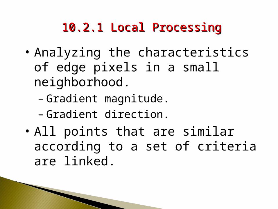
10.2.1 Local Processing10.2.1 Local Processing10.2.1 Local Processing10.2.1 Local Processing

• Analyzing the characteristics of edge pixels in a small neighborhood.– Gradient magnitude.– Gradient direction.

• All points that are similar according to a set of criteria are linked.

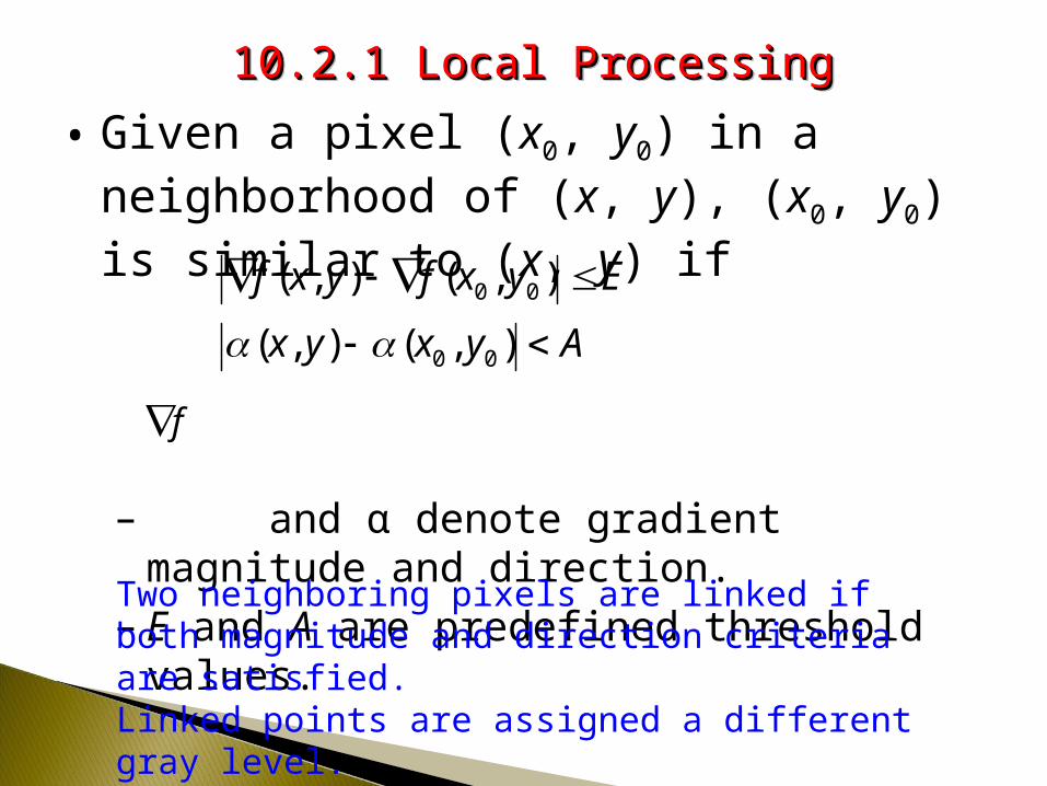
• Given a pixel (x0, y0) in a neighborhood of (x, y), (x0, y0) is similar to (x, y) if

– and α denote gradient magnitude and direction.

– E and A are predefined threshold values.

10.2.1 Local Processing10.2.1 Local Processing10.2.1 Local Processing10.2.1 Local Processing

Ayxyx

Eyxfyxf

),(),(

),(),(

00

00

f

Two neighboring pixels are linked if both magnitude and direction criteria are satisfied. Linked points are assigned a different gray level.

Example 10.6Example 10.6Example 10.6Example 10.6

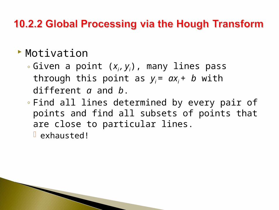
Motivation◦ Given a point (xi , yi), many lines pass through this point as

yi = axi + b with different a and b.

◦ Find all lines determined by every pair of points and find all subsets of points that are close to particular lines. exhausted!

The Parameter SpaceThe Parameter Space

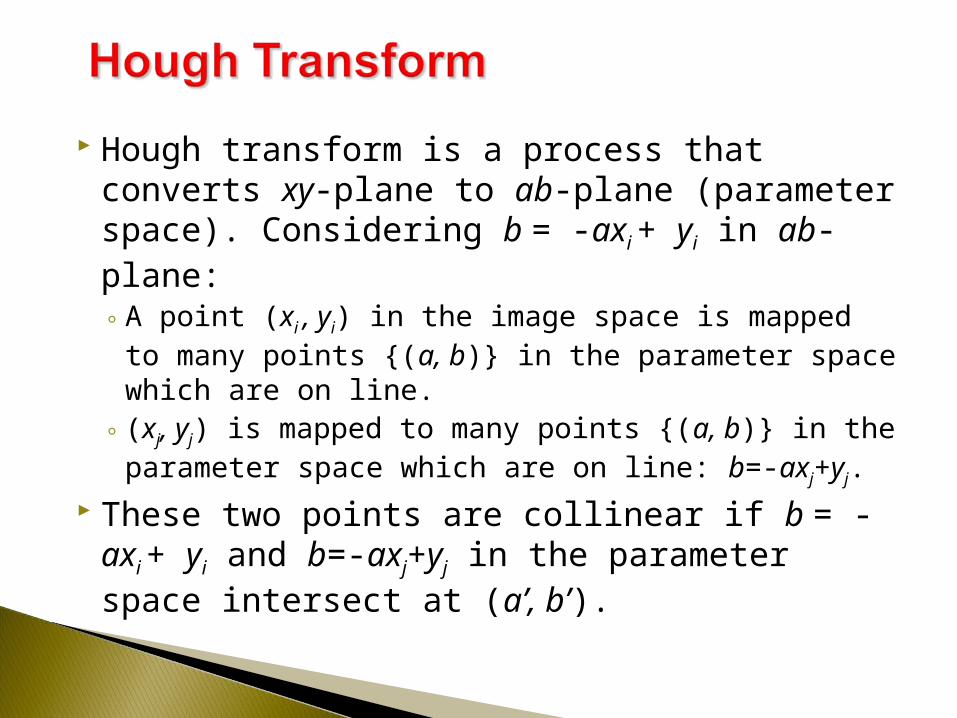
Hough transform is a process that converts xy-plane to ab-plane (parameter space). Considering b = -axi + yi in ab-plane:◦ A point (xi , yi) in the image space is mapped to many

points {(a, b)} in the parameter space which are on line.

◦ (xj, yj) is mapped to many points {(a, b)} in the parameter space which are on line: b=-axj+yj.

These two points are collinear if b = -axi + yi and b=-axj+yj in the parameter space intersect at (a’, b’).

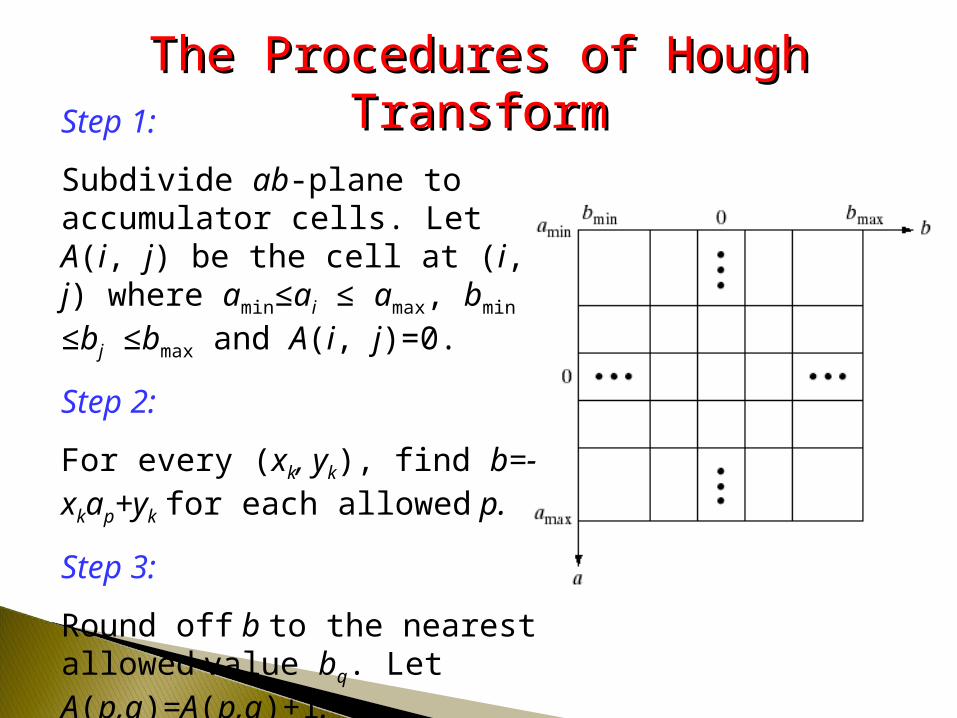
Step 1:

Subdivide ab-plane to accumulator cells. Let A(i, j) be the cell at (i, j) where amin≤ai ≤ amax, bmin ≤bj ≤bmax and A(i, j)=0.

Step 2:

For every (xk, yk), find b=-xkap+yk for each allowed p.

Step 3:

Round off b to the nearest allowed value bq. Let A(p,q)=A(p,q)+1.

The Procedures of Hough TransformThe Procedures of Hough Transform

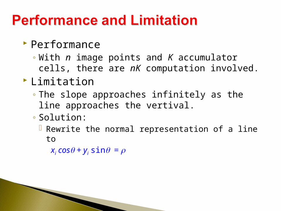
Performance◦ With n image points and K accumulator cells, there are

nK computation involved. Limitation

◦ The slope approaches infinitely as the line approaches the vertival.

◦ Solution: Rewrite the normal representation of a line to

xi cos + yi sin =

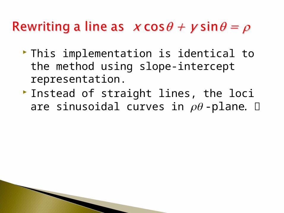
This implementation is identical to the method using slope-intercept representation.

Instead of straight lines, the loci are sinusoidal curves in -plane.

Rewriting a line as Rewriting a line as x x coscos + y + y sinsin = =

-90 90

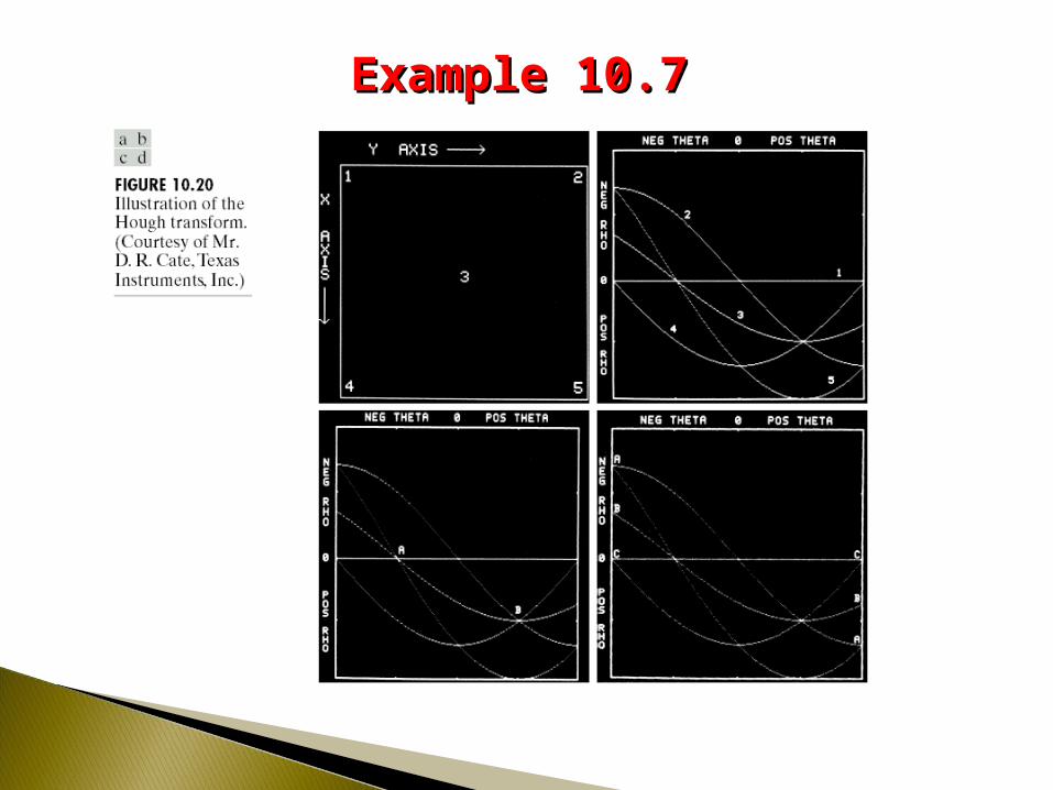
Example 10.7Example 10.7

1. Compute the gradient of an image and threshold it to obtain a binary image.

2. Specify subdivisions in the -plane.3. Examine the counts of the accumulator cells for

high pixel concentrations.4. Examine the relationship (for continuity)

between pixels in a chosen cell.

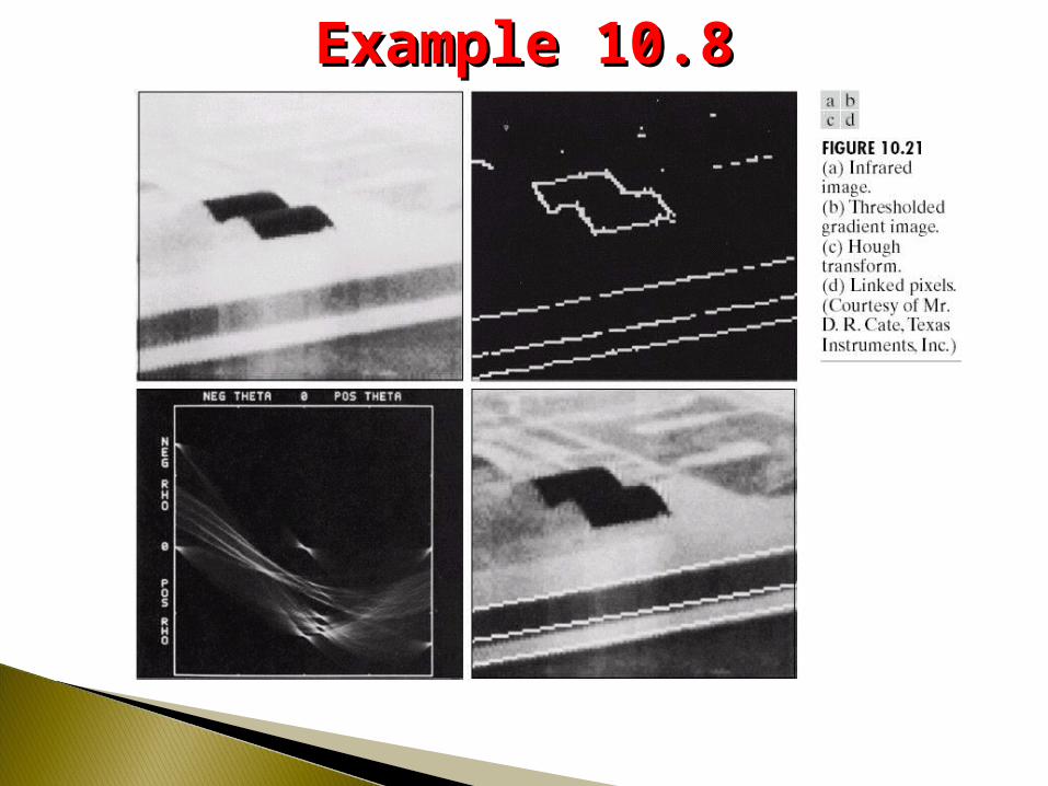
Example 10.8Example 10.8

Thresholding features its intuitive properties and simplicity in image segmentation.

Select a threshold T to separate the object pixels from background pixels.◦ Any point (x, y) with f(x,y) > T is called an object

point (labeled 1); otherwise, the point is called a background point (labeled 0).

◦ For multilevel thresholding, classify (x,y) as belongs to one object class if T1 < f(x,y) T2, to the other object class if f(x, y) > T2, and to the background f(x, y) T1.

10.3.1 Foundation

The threshold T can be viewed as an operation in the following form:

T = T[x, y, p(x,y), f(x,y)]where p(x,y) denotes some local property of this point (x, y), ◦ For example, the average level of a neighborhood centered

on (x, y). If T depends…

◦ only on f(x, y), then it is called global.◦ both on f(x, y) and p(x,y), then it is called local. ◦ Not only on f(x, y) and p(x,y), but on x and y, then it is called

dynamic or adaptive.

10.3.1 Foundation

Example 10.10Example 10.10

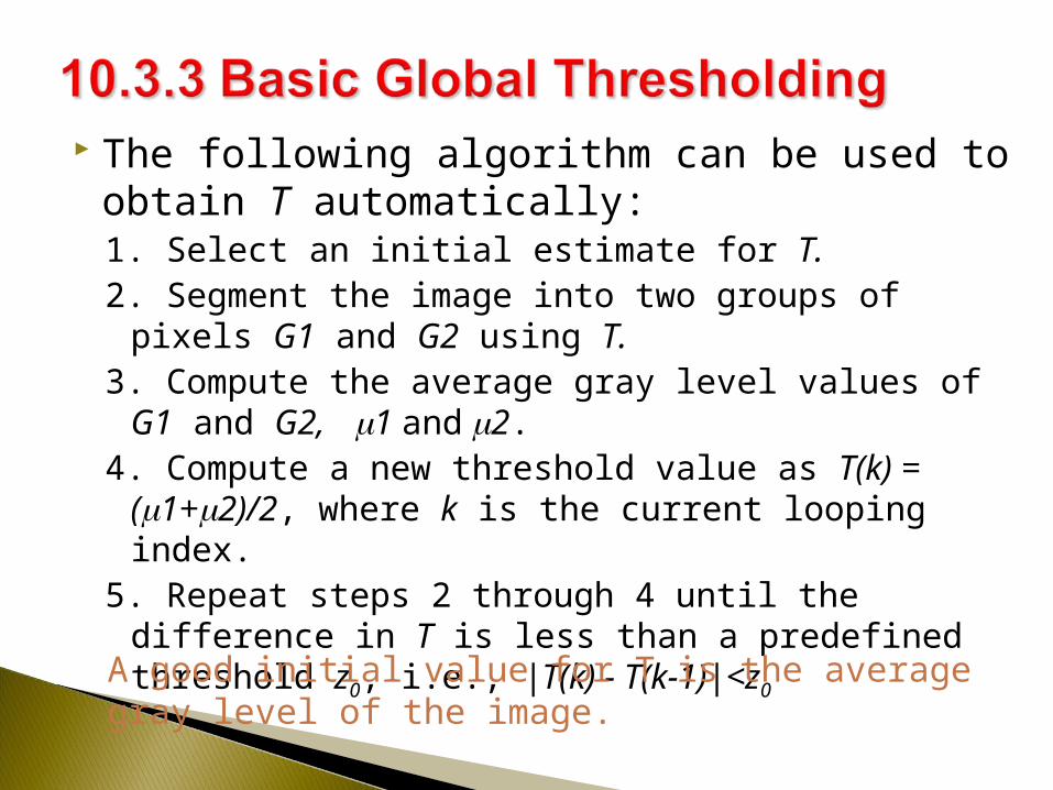
The following algorithm can be used to obtain T automatically:1. Select an initial estimate for T.2. Segment the image into two groups of pixels G1 and G2

using T.3. Compute the average gray level values of G1 and G2,

1 and 2.4. Compute a new threshold value as T(k) = (1+2)/2,

where k is the current looping index.5. Repeat steps 2 through 4 until the difference in T is less

than a predefined threshold z0, i.e., |T(k) - T(k-1)|<z0

A good initial value for T is the average gray level of the image.

Example 10.11Example 10.11

Three iteration.

The resulted threshold value is 125.4

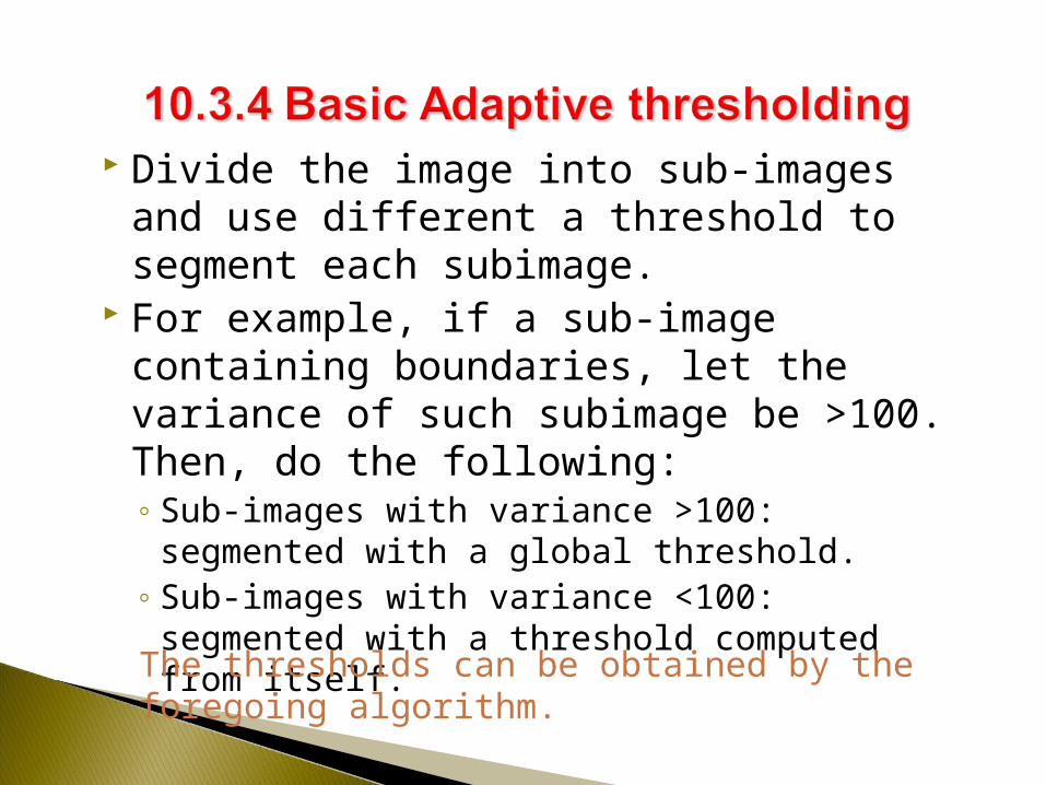
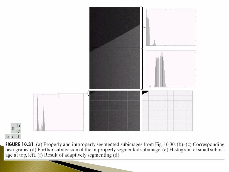
Divide the image into sub-images and use different a threshold to segment each subimage.

For example, if a sub-image containing boundaries, let the variance of such subimage be >100. Then, do the following:◦ Sub-images with variance >100: segmented with a

global threshold.◦ Sub-images with variance <100: segmented with a

threshold computed from itself.

The thresholds can be obtained by the foregoing algorithm.

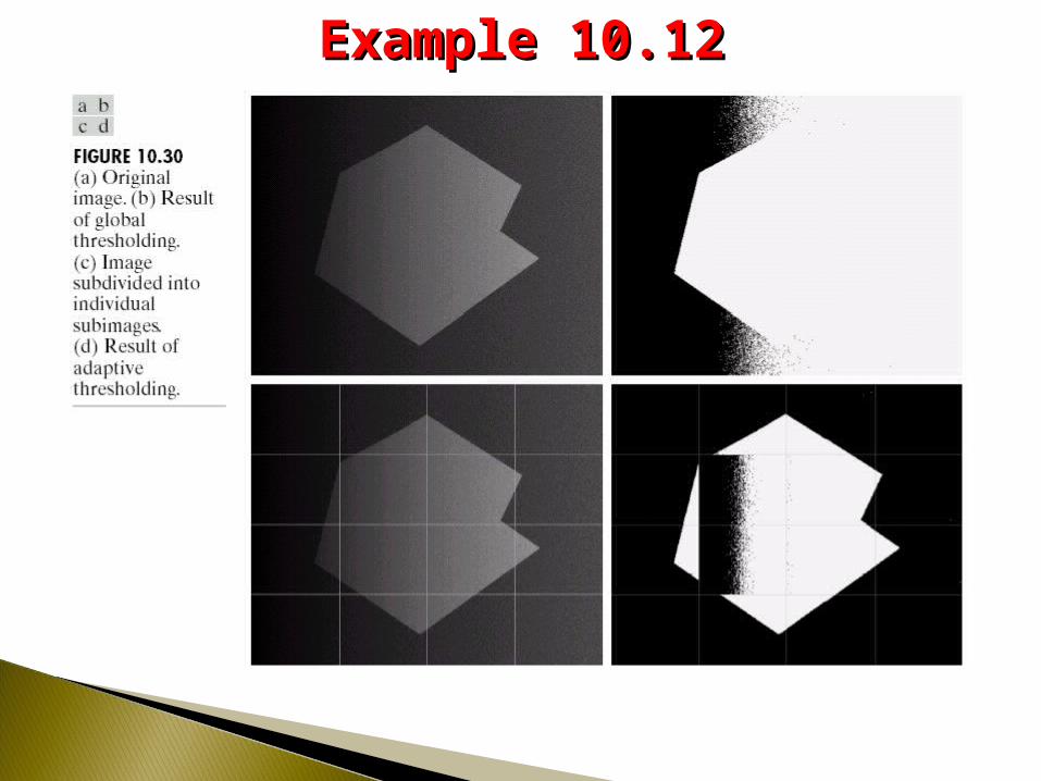
Example 10.12Example 10.12

Consider only those pixels that lie on or near the edges between objects and background.

To form a three-level image s(x, y), let:

◦ For pixels not on edges, s(x,y) = 0.◦ For pixels on dark side of edges, s(x,y) = +.◦ For pixels not on light side of edges, s(x,y) = –.

0

0

0

),(2

2

fandTfif

fandTfif

Tfif

yxs

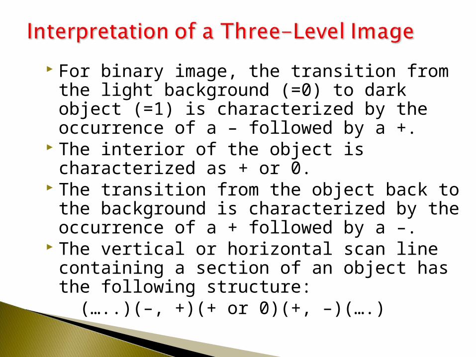
For binary image, the transition from the light background (=0) to dark object (=1) is characterized by the occurrence of a – followed by a +.

The interior of the object is characterized as + or 0.

The transition from the object back to the background is characterized by the occurrence of a + followed by a –.

The vertical or horizontal scan line containing a section of an object has the following structure: (…..)(–, +)(+ or 0)(+, –)(….)

Example 10.14Example 10.14• Segmenting an image using a histogram of

the gradient and Laplacian.

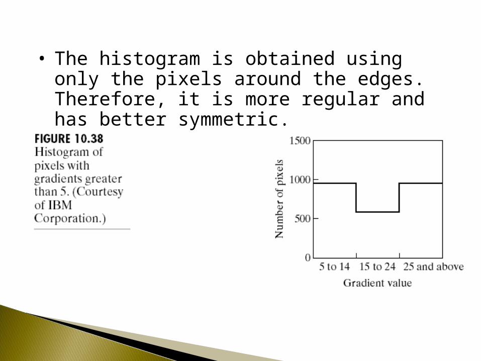
• The histogram is obtained using only the pixels around the edges. Therefore, it is more regular and has better symmetric.

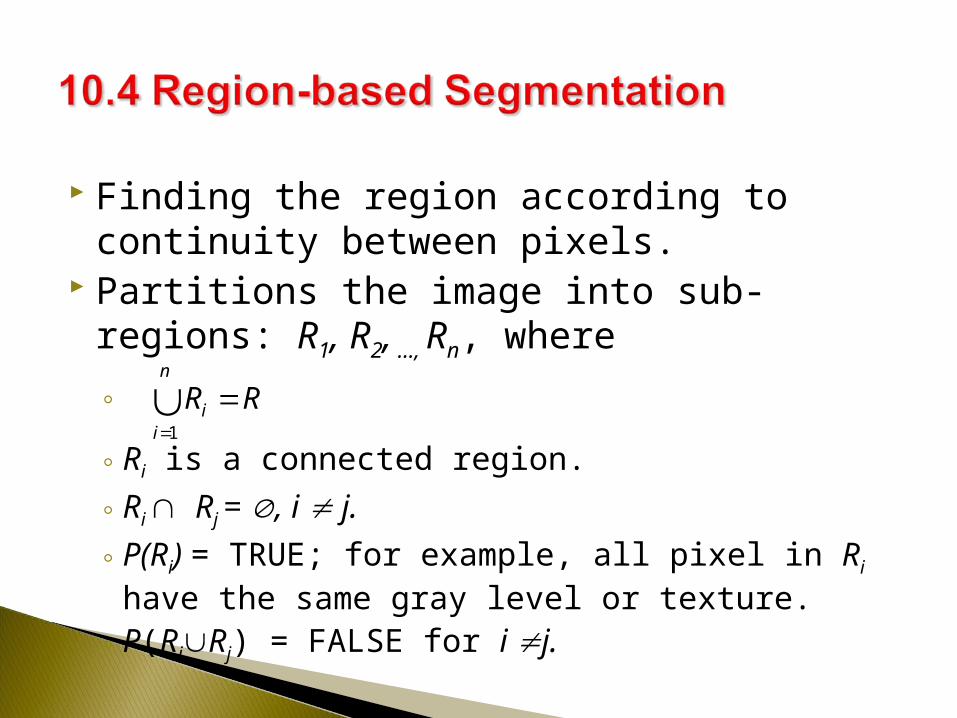
Finding the region according to continuity between pixels.

Partitions the image into sub-regions: R1, R2, ...,

Rn, where

◦

◦ Ri is a connected region.

◦ Ri Rj = , i j.

◦ P(Ri) = TRUE; for example, all pixel in Ri have the same gray level or texture.

◦ P(RiRj) = FALSE for i j.

RRn

ii

1

Finding the region according to continuity between pixels.◦ The basic approach is to start with a set of “seeds”,

and then grow regions by appending to each seed those neighboring points.

The selection of seeds◦ Manually

A procedure that groups pixels or subregions into larger regions based on predefined criteria.

Starting with a set of “seeds” and then appending to each seed those neighboring pixels that have properties similar to the seed.◦ such as specified gray-level or color.

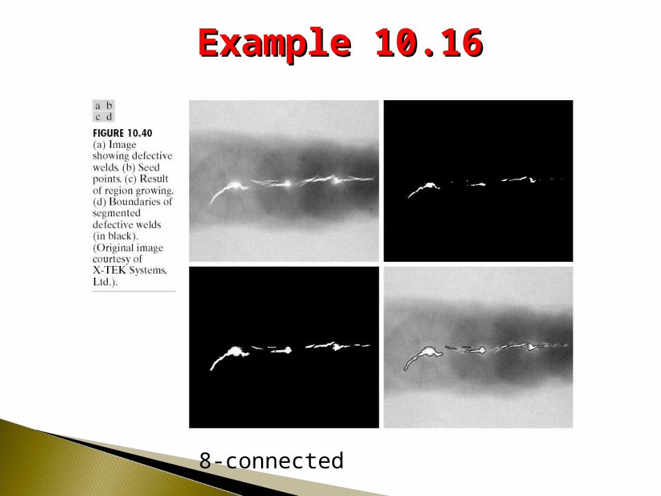
Example 10.16Example 10.16

8-connected

• As shown below, even with well-behaved histograms, multilevel thresholding is difficult.

• Solving this problem using region-based approach may be a good way in dealing with this problem.

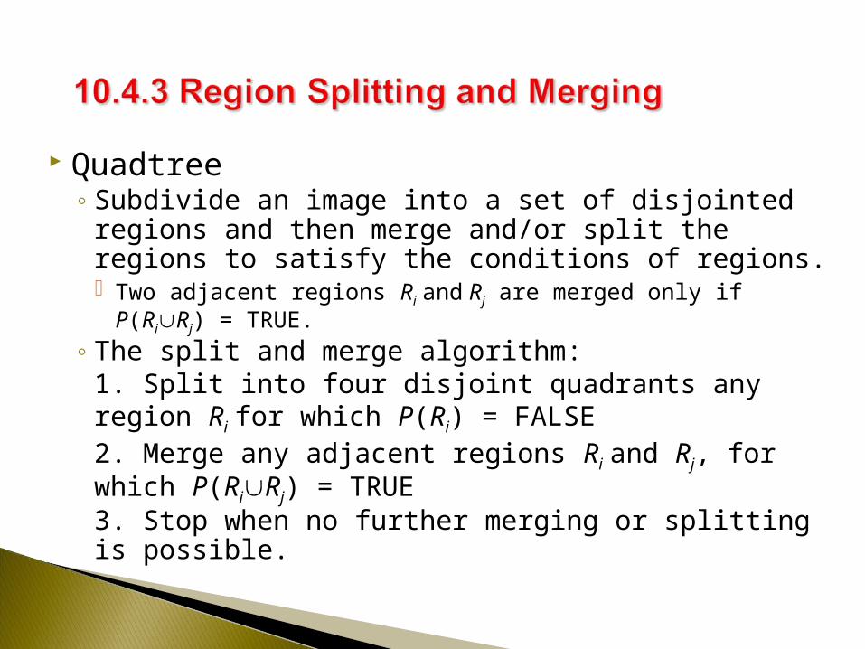
Quadtree◦ Subdivide an image into a set of disjointed regions and

then merge and/or split the regions to satisfy the conditions of regions. Two adjacent regions Ri and Rj are merged only if P(RiRj) =

TRUE.◦ The split and merge algorithm:

1. Split into four disjoint quadrants any region Ri for which P(Ri) = FALSE2. Merge any adjacent regions Ri and Rj, for which P(RiRj) = TRUE3. Stop when no further merging or splitting is possible.

A quadtree representation

The Construction of a QuadtreeThe Construction of a Quadtree

• P(RiRj) = TRUE can be defined as follows: If P(Ri) = TRUE, then in Ri, 80% of the pixels in it have the property: |zj-mi|≤σi .

Example 10.17Example 10.17