Chapter 10: Curves and Surfaces Part 1 E. Angel and D. Shreiner: Interactive Computer Graphics 6E © Addison-Wesley 2012 1 Mohan Sridharan Based on Slides.

Chapter 10: Curves and SurfacesPart 1

E. Angel and D. Shreiner: Interactive Computer Graphics 6E © Addison-Wesley

20121

Mohan SridharanBased on Slides by Edward Angel and Dave Shreiner

Objectives

• Introduce types of curves and surfaces:– Explicit.– Implicit.– Parametric.– Strengths and weaknesses.

• Discuss Modeling and Approximations:– Conditions.– Stability.


20122

Escaping Flatland

• Until now we have worked with flat entities such as lines and polygons:– Fit well with graphics hardware.– Mathematically simple.

• The world is not composed of flat entities:– Need curves and curved surfaces.– May only have need at the application level.– Implementation can render them approximately with flat primitives.


20123

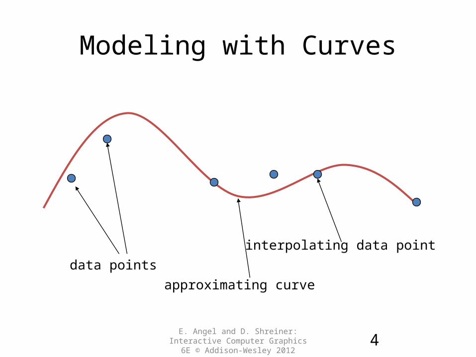
Modeling with Curves


20124

data points

approximating curve

interpolating data point

What Makes a Good Representation?

• There are many ways to represent curves and surfaces.

• Want a representation that is:– Stable.– Smooth.– Easy to evaluate.– Must we interpolate or can we just come close to data?– Do we need derivatives?


20125

Explicit Representation

• Dependent variables in terms of independent variables.• Familiar form of curve in 2D:

y=f(x)

• Coordinate system dependent.• Cannot represent all curves (special cases):

– Vertical lines and circles.

• Extension to 3D :– y=f(x), z=g(x)

– The form z = f(x, y) defines a surface.


20126

x

y

x

y

z

Implicit Representation

• Two dimensional curve(s): f(x, y)=0

• Much more robust (less coordinate system dependent):– All lines ax+by+c=0; Circles x2+y2-r2=0

• Divides space into points that belong to curve and those that do not.

• Three dimensions f(x, y, z)=0 defines a surface:– Intersect two surface to get a curve.

• In general, difficult to solve for points that satisfy constraints.


20127

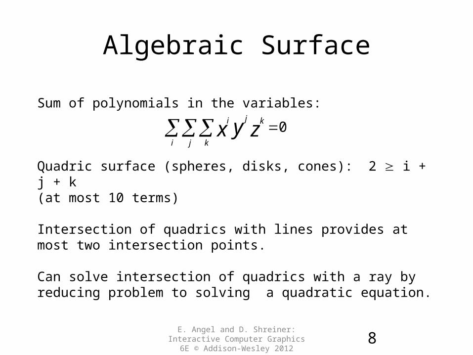
Algebraic Surface


20128

0 zyxkj

i j k

i

Sum of polynomials in the variables:

Quadric surface (spheres, disks, cones): 2 i + j + k(at most 10 terms)

Intersection of quadrics with lines provides at most two intersection points.

Can solve intersection of quadrics with a ray by reducing problem to solving a quadratic equation.

Parametric Curves

• Separate equation for each spatial variable in terms of an independent variable/parameter (u). x=x(u)

y=y(u)

z=z(u)

• For umax u umin we trace out a curve in two or three dimensions:


20129

Locus of points: p(u)=[x(u), y(u), z(u)]T

p(u)

p(umin)

p(umax)

Selecting Functions

• Usually we can select “good” functions:– Not unique for a given spatial curve.– Approximate or interpolate known data.

– Want functions that are easy to evaluate.– Want functions that are easy to differentiate:

• Computation of normals.• Connecting pieces (segments).

– Want functions that are smooth.


201210

Parametric Lines


201211

p(u)=(1-u)p0+up1

We can normalize u to be over the interval (0,1).

Line connecting two points p0 and p1:

Ray from p0 in the direction d:

p(0) = p0

p(1)= p1

p(u)=p0+udp(0) = p0

p(1)= p0 +d

d

Parametric Surfaces

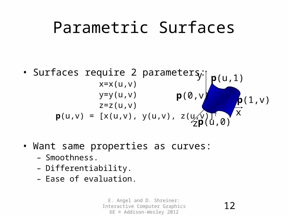
• Surfaces require 2 parameters: x=x(u,v) y=y(u,v) z=z(u,v) p(u,v) = [x(u,v), y(u,v), z(u,v)]T

• Want same properties as curves: – Smoothness.– Differentiability.– Ease of evaluation.


201212

x

y

z p(u,0)

p(1,v)p(0,v)

p(u,1)

Surface Normals

• We can differentiate with respect to u and v to obtain the normal at any point p.


201213

uvu

uvu

uvu

u

vu

/),(z

/),(y

/),(x),(p

vvu

vvu

vvu

v

vu

/),(z

/),(y

/),(x),(p

v

vu

u

vu

),(),( ppn

Parametric Planes


201214

Point-vector form:

p(u,v)=p0+uq+vr

n = q x r

Three-point form:

q

r

p0

n

p0

n

p1

p2

q = p1 – p0

r = p2 – p0

Parametric Sphere


201215

x(u,v) = r cos sin y(u,v) = r sin sin z(u,v) = r cos

360 0180 0

constant: circles of constant longitude. constant: circles of constant latitude.

differentiate to show n = p

Curve Segments

• After normalizing u, each curve is written as: p(u)=[x(u), y(u), z(u)]T, 1 u 0

• Classical numerical methods design a single global curve.• In computer graphics and CAD, it is better to design small

connected curve segments.


201216

p(u)

q(u)p(0)q(1)

join point p(1) = q(0)

Parametric Polynomial Curves


201217

ucux iN

ixi

0

)( ucuy jM

jyj

0

)( ucuz kL

kzk

0

)(

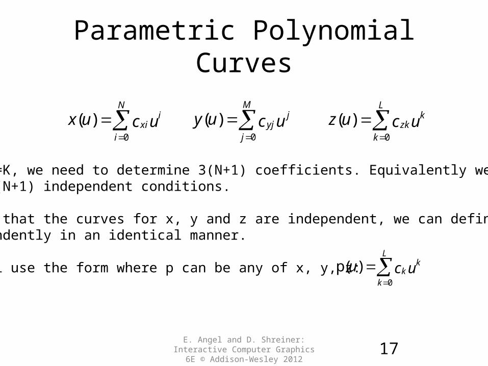
If N=M=K, we need to determine 3(N+1) coefficients. Equivalently we need 3(N+1) independent conditions.

Noting that the curves for x, y and z are independent, we can define each independently in an identical manner.

We will use the form where p can be any of x, y, z: ucu kL

kk

0

)(p

Why Polynomials?

• Easy to evaluate.

• Continuous and differentiable everywhere:– Must worry about continuity at join points including continuity of

derivatives.


201218

p(u)

q(u)

join point p(1) = q(0)but p’(1) q’(0)

Cubic Parametric Polynomials

• N=M=L=3, balances ease of evaluation and flexibility in design:

• Four coefficients to determine for each of x, y and z.

• Seek four independent conditions for various values of u resulting in 4 equations in 4 unknowns for each of x, y and z.– Conditions are a mixture of continuity requirements at the join

points and conditions for fitting the data.


201219

ucu k

kk

3

0

)(p

Cubic Polynomial Surfaces


201220

General equations are of the form:

where:

p is any of x, y or z.

Need 48 coefficients (3 independent sets of 16) to determine a surface patch.

p(u,v)=[x(u,v), y(u,v), z(u,v)]T

vucvu ji

i jij

3

0

3

0

),(p

Objectives

• Introduce the types of curves:– Interpolating.– Hermite.– Bezier.– B-splines.

• Analyze their performance.


201221

Design Criteria

• Criteria for designing parametric polynomials:– Local control of shape.

– Smoothness and continuity.

– Ability to evaluate derivatives.

– Stability.

– Ease of rendering.


201222

Matrix-Vector Form


201223

ucu k

kk

3

0

)(p

c

c

c

c

3

2

1

0

c

u

u

u

3

2

1

uDefine

uccu TTu )(pThen

Interpolating Curve


201224

p0

p1

p2

p3

Cubic interpolating polynomial: an example of the cubic parametric polynomial.

Given four data (control) points p0 , p1 ,p2 , p3 determine cubic p(u) which passes through them.

Must find: c0 ,c1 ,c2 , c3

Interpolation Equations


201225

Apply the interpolating conditions at u=0, 1/3, 2/3, 1.p0 = p(0) = c0

p1 = p(1/3) = c0+(1/3)c1+(1/3)2c2+(1/3)3c2

p2 = p(2/3) = c0+(2/3)c1+(2/3)2c2+(2/3)3c2

p3 = p(1) = c0+c1+c2+c3

or in matrix form with p = [p0 p1 p2 p3]T

p=Ac

11113

2

3

2

3

21

3

1

3

1

3

11

0001

32

32

A

Interpolation Matrix


201226

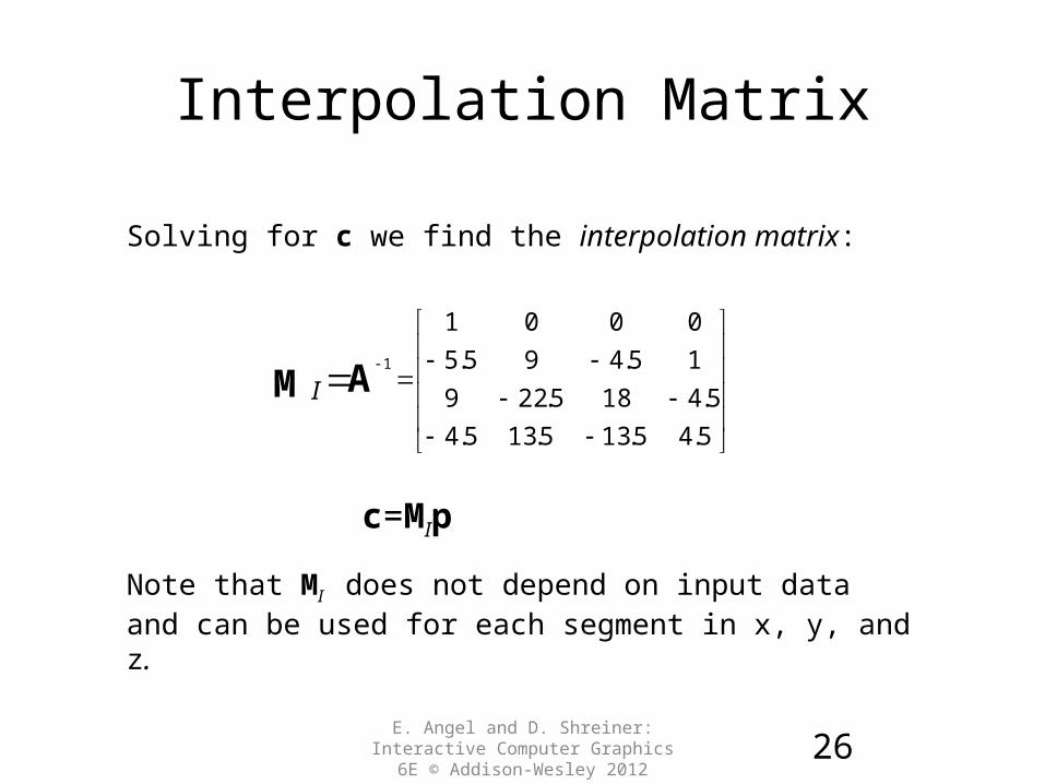
Solving for c we find the interpolation matrix:

Note that MI does not depend on input data and can be used for each segment in x, y, and z.

5.45.135.135.4

5.4185.229

15.495.5

0001

1

AMI

c=MIp

Interpolating Multiple Segments


201227

use p = [p0 p1 p2 p3]T use p = [p3 p4 p5 p6]T

Derive a set of cubic interpolating curves, each specified with four control points.

Get C0 continuity at join points but not C1 continuity of derivatives!

Blending Functions


201228

Study smoothness of interpolating polynomial curves by rewriting the equation for p(u):

p(u) = uTc = uTMIp = b(u)Tp

where b(u) = [b0(u) b1(u) b2(u) b3(u)]T is an array of blending polynomials such that:p(u) = b0(u)p0+ b1(u)p1+ b2(u)p2+ b3(u)p3

b0(u) = -4.5(u-1/3)(u-2/3)(u-1)b1(u) = 13.5u (u-2/3)(u-1)b2(u) = -13.5u (u-1/3)(u-1)b3(u) = 4.5u (u-1/3)(u-2/3)

Blending Functions

• These functions are not smooth:– Hence the interpolation polynomial is not smooth!

– Lack of smoothness because curves have to pass through control points.– More pronounced for higher degree polynomials.– Also lack derivative continuity at joint points. – Limited use in CG applications.


201229

Cubic Interpolating Patch


201230

vucvup j

jij

i

oi

3

0

3

),(

Need 16 conditions to determine the 16 coefficients cij

Choose at u, v = 0, 1/3, 2/3, 1

Matrix Form


201231

Define v = [1 v v2 v3]T C = [cij] P = [pij]

p(u,v) = uTCv

If we observe that for constant u (v), we obtain interpolating curve in v (u), we can show:

C=MIPMI

p(u,v) = uTMIPMITv

Blending Patches


201232

pvbubvup ijjj

ioi

)()(),(3

0

3

Each bi(u)bj(v) is a blending patch.

We can therefore build and analyze surfaces from our knowledge of curves.

Other Types of Curves and Surfaces

• How to get around the limitations of the interpolating form?– Lack of smoothness.– Discontinuous derivatives at join points.

• We have four conditions (for cubics) applied to each segment:– Use them other than for interpolation.– Need only come close to the data!


201233

Hermite Form


201234

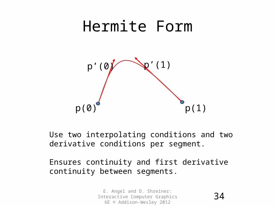
p(0) p(1)

p’(0) p’(1)

Use two interpolating conditions and two derivative conditions per segment.

Ensures continuity and first derivative continuity between segments.

Equations


201235

Interpolating conditions are the same at ends:

p(0) = p0 = c0

p(1) = p3 = c0+c1+c2+c3

Differentiating we find p’(u) = c1+2uc2+3u2c3. Evaluating at end points:

p’(0) = p’0 = c1

p’(1) = p’3 = c1+2c2+3c3

Matrix Form


201236

cq

3210

0010

1111

0001

p'

p'

p

p

3

0

3

0

Solving, we find c = MHq where MH is the Hermite matrix.

1122

1233

0100

0001

MH

Blending Polynomials


201237

p(u) = b(u)Tq

uu

uuu

uu

uu

u

23

23

23

23

2

32

132

)(b

These functions are smooth, but the Hermite form is not used directly in Computer Graphics and CAD.

We usually have control points but not derivatives.

However, the Hermite form is the basis of the Bezier form.

Parametric and Geometric Continuity

• We can require the derivatives of x, y and z to be continuous at join points (C0 and C1 parametric continuity).

• Alternately, we can only require that the tangents of the resulting curve be continuous, i.e., proportional but different magnitudes (G1 geometry continuity).

• The latter gives more flexibility as we have need satisfy only two conditions rather than three at each join point.


201238

)0(

)0(

)0(

)0(

)1(

)1(

)1(

)1(

z

y

x

z

y

x

q

q

q

p

p

p

qp

)0(

)0(

)0(

)0(

)1(

)1(

)1(

)1('

'

'

'

'

'

'

'

z

y

x

z

y

x

q

q

q

p

p

p

qp

)0()1( '' qp

Example

• Here the p and q have the same tangents at the ends of the segment.• Curves have different derivatives (same direction, different magnitude).

• Generate different Hermite curves.

• This techniques is used in drawing applications.


201239

Higher Dimensional Approximations

• The techniques for both interpolating and Hermite curves can be used with higher dimensional parametric polynomials.

• For interpolating form, the resulting matrix becomes increasingly more ill-conditioned and the resulting curves less smooth and more prone to numerical errors.

• In both cases, there is more work in rendering the resulting polynomial curves and surfaces.


201240

Chapter 10: Curves and Surfaces Part 1 E. Angel and D. Shreiner: Interactive Computer Graphics 6E © Addison-Wesley 2012 1 Mohan Sridharan Based on Slides.

Documents

interactive computer

e addisonwesley

dave shreiner slide

x y x y z slide

graphics hardware

edward angel

pu max slide

data point slide