Chapter 10 Correlation and Regression Our interest in this chapter is in situations in which we can associate to each element of a population or sample two measurements x and y, particularly in the case that it is of interest to use the value of x to predict the value of y. For example, the population could be the air in automobile garages, x could be the electrical current produced by an electrochemical reaction taking place in a carbon monoxide meter, and y the concentration of carbon monoxide in the air. In this chapter we will learn statistical methods for analyzing the relationship between variables x and y in this context. A list of all the formulas that appear anywhere in this chapter are collected in the last section for ease of reference. 531

Welcome message from author
This document is posted to help you gain knowledge. Please leave a comment to let me know what you think about it! Share it to your friends and learn new things together.
Transcript

Chapter 10
Correlation and Regression
Our interest in this chapter is in situations in which we can associate to eachelement of a population or sample two measurements x and y, particularly in thecase that it is of interest to use the value of x to predict the value of y. For example,the population could be the air in automobile garages, x could be the electricalcurrent produced by an electrochemical reaction taking place in a carbon monoxidemeter, and y the concentration of carbon monoxide in the air. In this chapter wewill learn statistical methods for analyzing the relationship between variables x andy in this context.
A list of all the formulas that appear anywhere in this chapter are collected in thelast section for ease of reference.
531
10.1 Linear Relationships Between Variables
LEARNING OBJECTIVE
1. To learn what it means for two variables to exhibit a relationship that isclose to linear but which contains an element of randomness.
The following table gives examples of the kinds of pairs of variables which could beof interest from a statistical point of view.
x y
Predictor or independent variableResponse or dependentvariable
Temperature in degrees CelsiusTemperature in degreesFahrenheit
Area of a house (sq.ft.) Value of the house
Age of a particular make and model car Resale value of the car
Amount spent by a business on advertisingin a year
Revenue received that year
Height of a 25-year-old man Weight of the man
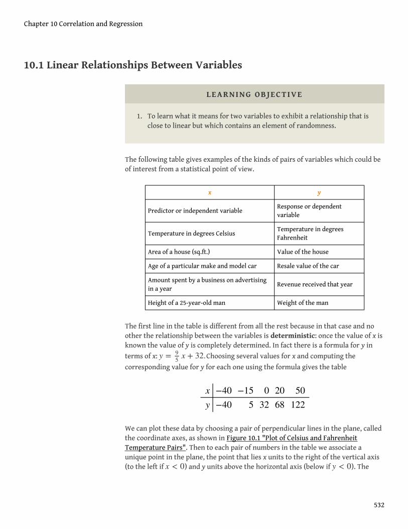
The first line in the table is different from all the rest because in that case and noother the relationship between the variables is deterministic: once the value of x isknown the value of y is completely determined. In fact there is a formula for y in
terms of x: y = 95 x + 32.Choosing several values for x and computing the
corresponding value for y for each one using the formula gives the table
We can plot these data by choosing a pair of perpendicular lines in the plane, calledthe coordinate axes, as shown in Figure 10.1 "Plot of Celsius and FahrenheitTemperature Pairs". Then to each pair of numbers in the table we associate aunique point in the plane, the point that lies x units to the right of the vertical axis(to the left if x < 0) and y units above the horizontal axis (below if y < 0). The
x
y
−40−40
−155
032
2068
50122
Chapter 10 Correlation and Regression
532

relationship between x and y is called a linear relationship because the points so
plotted all lie on a single straight line. The number 95 in the equation y = 9
5 x + 32is the slope of the line, and measures its steepness. It describes how y changes in
response to a change in x: if x increases by 1 unit then y increases (since 95 is
positive) by 95 unit. If the slope had been negative then y would have decreased in
response to an increase in x. The number 32 in the formula y = 95 x + 32 is the y-
intercept of the line; it identifies where the line crosses the y-axis. You may recallfrom an earlier course that every non-vertical line in the plane is described by anequation of the form y = mx + b , where m is the slope of the line and b is its y-intercept.
Figure 10.1 Plot of Celsius and Fahrenheit Temperature Pairs
The relationship between x and y in the temperature example is deterministicbecause once the value of x is known, the value of y is completely determined. Incontrast, all the other relationships listed in the table above have an element ofrandomness in them. Consider the relationship described in the last line of thetable, the height x of a man aged 25 and his weight y. If we were to randomly selectseveral 25-year-old men and measure the height and weight of each one, we mightobtain a collection of (x, y) pairs something like this:
Chapter 10 Correlation and Regression
10.1 Linear Relationships Between Variables 533
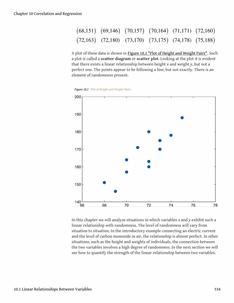
A plot of these data is shown in Figure 10.2 "Plot of Height and Weight Pairs". Sucha plot is called a scatter diagram or scatter plot. Looking at the plot it is evidentthat there exists a linear relationship between height x and weight y, but not aperfect one. The points appear to be following a line, but not exactly. There is anelement of randomness present.
Figure 10.2 Plot of Height and Weight Pairs
In this chapter we will analyze situations in which variables x and y exhibit such alinear relationship with randomness. The level of randomness will vary fromsituation to situation. In the introductory example connecting an electric currentand the level of carbon monoxide in air, the relationship is almost perfect. In othersituations, such as the height and weights of individuals, the connection betweenthe two variables involves a high degree of randomness. In the next section we willsee how to quantify the strength of the linear relationship between two variables.
(68,151)(72,163)
(69,146)(72,180)
(70,157)(73,170)
(70,164)(73,175)
(71,171)
(74,178)(72,160)(75,188)
Chapter 10 Correlation and Regression
10.1 Linear Relationships Between Variables 534
KEY TAKEAWAYS
• Two variables x and y have a deterministic linear relationship if points
plotted from (x, y) pairs lie exactly along a single straight line.
• In practice it is common for two variables to exhibit a relationship thatis close to linear but which contains an element, possibly large, ofrandomness.
Chapter 10 Correlation and Regression
10.1 Linear Relationships Between Variables 535
EXERCISES
BASIC
1. A line has equation y = 0.5x + 2.a. Pick five distinct x-values, use the equation to compute the corresponding
y-values, and plot the five points obtained.b. Give the value of the slope of the line; give the value of the y-intercept.
2. A line has equation y = x−0.5.a. Pick five distinct x-values, use the equation to compute the corresponding
y-values, and plot the five points obtained.b. Give the value of the slope of the line; give the value of the y-intercept.
3. A line has equation y = −2x + 4.a. Pick five distinct x-values, use the equation to compute the corresponding
y-values, and plot the five points obtained.b. Give the value of the slope of the line; give the value of the y-intercept.
4. A line has equation y = −1.5x + 1.a. Pick five distinct x-values, use the equation to compute the corresponding
y-values, and plot the five points obtained.b. Give the value of the slope of the line; give the value of the y-intercept.
5. Based on the information given about a line, determine how y will change(increase, decrease, or stay the same) when x is increased, and explain. In somecases it might be impossible to tell from the information given.
a. The slope is positive.b. The y-intercept is positive.c. The slope is zero.
6. Based on the information given about a line, determine how y will change(increase, decrease, or stay the same) when x is increased, and explain. In somecases it might be impossible to tell from the information given.
a. The y-intercept is negative.b. The y-intercept is zero.c. The slope is negative.
7. A data set consists of eight (x, y) pairs of numbers:
Chapter 10 Correlation and Regression
10.1 Linear Relationships Between Variables 536
a. Plot the data in a scatter diagram.b. Based on the plot, explain whether the relationship between x and y
appears to be deterministic or to involve randomness.c. Based on the plot, explain whether the relationship between x and y
appears to be linear or not linear.
8. A data set consists of ten (x, y) pairs of numbers:
a. Plot the data in a scatter diagram.b. Based on the plot, explain whether the relationship between x and y
appears to be deterministic or to involve randomness.c. Based on the plot, explain whether the relationship between x and y
appears to be linear or not linear.
9. A data set consists of nine (x, y) pairs of numbers:
a. Plot the data in a scatter diagram.b. Based on the plot, explain whether the relationship between x and y
appears to be deterministic or to involve randomness.c. Based on the plot, explain whether the relationship between x and y
appears to be linear or not linear.
10. A data set consists of five (x, y) pairs of numbers:
a. Plot the data in a scatter diagram.b. Based on the plot, explain whether the relationship between x and y
appears to be deterministic or to involve randomness.c. Based on the plot, explain whether the relationship between x and y
appears to be linear or not linear.
(0,12)
(2,15)(4,16)(5,14)
(8,22)
(13,24)(15,28)(20,30)
(3,20)
(5,13)(6,9)(8,4)
(11,0)
(12,0)
(14,1)
(17,6)(18,9)
(20,16)
(8,16)(9,9)
(10,4)(11,1)
(12,0)(13,1)
(14,4)(15,9)
(16,16)
(0,1) (2,5) (3,7) (5,11) (8,17)
Chapter 10 Correlation and Regression
10.1 Linear Relationships Between Variables 537
APPLICATIONS
11. At 60°F a particular blend of automotive gasoline weights 6.17 lb/gal. Theweight y of gasoline on a tank truck that is loaded with x gallons of gasoline isgiven by the linear equation
a. Explain whether the relationship between the weight y and the amount xof gasoline is deterministic or contains an element of randomness.
b. Predict the weight of gasoline on a tank truck that has just been loadedwith 6,750 gallons of gasoline.
12. The rate for renting a motor scooter for one day at a beach resort area is $25plus 30 cents for each mile the scooter is driven. The total cost y in dollars forrenting a scooter and driving it x miles is
a. Explain whether the relationship between the cost y of renting the scooterfor a day and the distance x that the scooter is driven that day isdeterministic or contains an element of randomness.
b. A person intends to rent a scooter one day for a trip to an attraction 17miles away. Assuming that the total distance the scooter is driven is 34miles, predict the cost of the rental.
13. The pricing schedule for labor on a service call by an elevator repair companyis $150 plus $50 per hour on site.
a. Write down the linear equation that relates the labor cost y to the numberof hours x that the repairman is on site.
b. Calculate the labor cost for a service call that lasts 2.5 hours.
14. The cost of a telephone call made through a leased line service is 2.5 cents perminute.
a. Write down the linear equation that relates the cost y (in cents) of a call toits length x.
b. Calculate the cost of a call that lasts 23 minutes.
LARGE DATA SET EXERCISES
15. Large Data Set 1 lists the SAT scores and GPAs of 1,000 students. Plot thescatter diagram with SAT score as the independent variable (x) and GPA as thedependent variable (y). Comment on the appearance and strength of any lineartrend.
y = 6.17x
y = 0.30x + 25
Chapter 10 Correlation and Regression
10.1 Linear Relationships Between Variables 538
http://www.gone.2012books.lardbucket.org/sites/all/files/data1.xls
16. Large Data Set 12 lists the golf scores on one round of golf for 75 golfers firstusing their own original clubs, then using clubs of a new, experimental design(after two months of familiarization with the new clubs). Plot the scatterdiagram with golf score using the original clubs as the independent variable (x)and golf score using the new clubs as the dependent variable (y). Comment onthe appearance and strength of any linear trend.
http://www.gone.2012books.lardbucket.org/sites/all/files/data12.xls
17. Large Data Set 13 records the number of bidders and sales price of a particulartype of antique grandfather clock at 60 auctions. Plot the scatter diagram withthe number of bidders at the auction as the independent variable (x) and thesales price as the dependent variable (y). Comment on the appearance andstrength of any linear trend.
http://www.gone.2012books.lardbucket.org/sites/all/files/data13.xls
Chapter 10 Correlation and Regression
10.1 Linear Relationships Between Variables 539
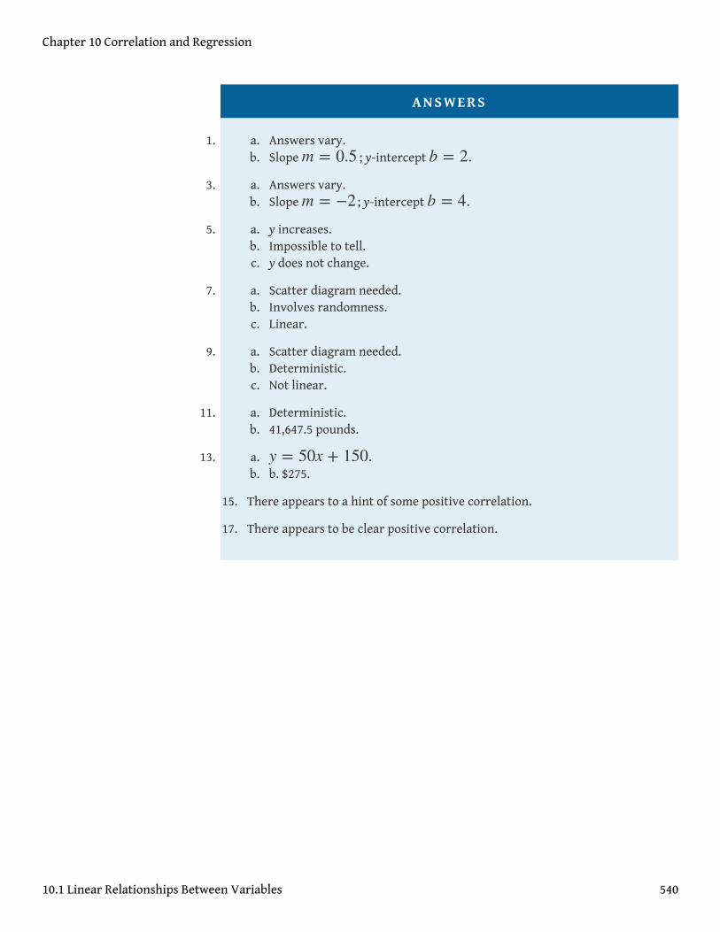
ANSWERS
1. a. Answers vary.b. Slope m = 0.5 ; y-intercept b = 2.
3. a. Answers vary.b. Slope m = −2 ; y-intercept b = 4.
5. a. y increases.b. Impossible to tell.c. y does not change.
7. a. Scatter diagram needed.b. Involves randomness.c. Linear.
9. a. Scatter diagram needed.b. Deterministic.c. Not linear.
11. a. Deterministic.b. 41,647.5 pounds.
13. a. y = 50x + 150.b. b. $275.
15. There appears to a hint of some positive correlation.
17. There appears to be clear positive correlation.
Chapter 10 Correlation and Regression
10.1 Linear Relationships Between Variables 540
10.2 The Linear Correlation Coefficient
LEARNING OBJECTIVE
1. To learn what the linear correlation coefficient is, how to compute it,and what it tells us about the relationship between two variables x and y.
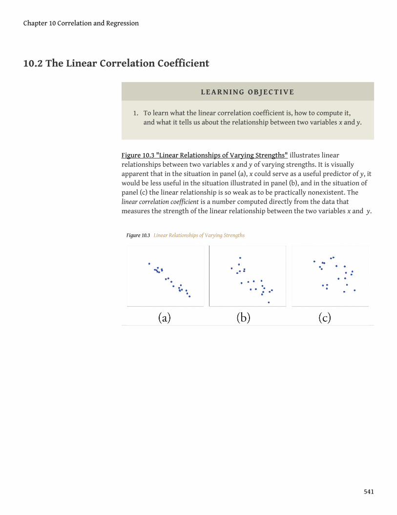
Figure 10.3 "Linear Relationships of Varying Strengths" illustrates linearrelationships between two variables x and y of varying strengths. It is visuallyapparent that in the situation in panel (a), x could serve as a useful predictor of y, itwould be less useful in the situation illustrated in panel (b), and in the situation ofpanel (c) the linear relationship is so weak as to be practically nonexistent. Thelinear correlation coefficient is a number computed directly from the data thatmeasures the strength of the linear relationship between the two variables x and y.
Figure 10.3 Linear Relationships of Varying Strengths
Chapter 10 Correlation and Regression
541
Definition
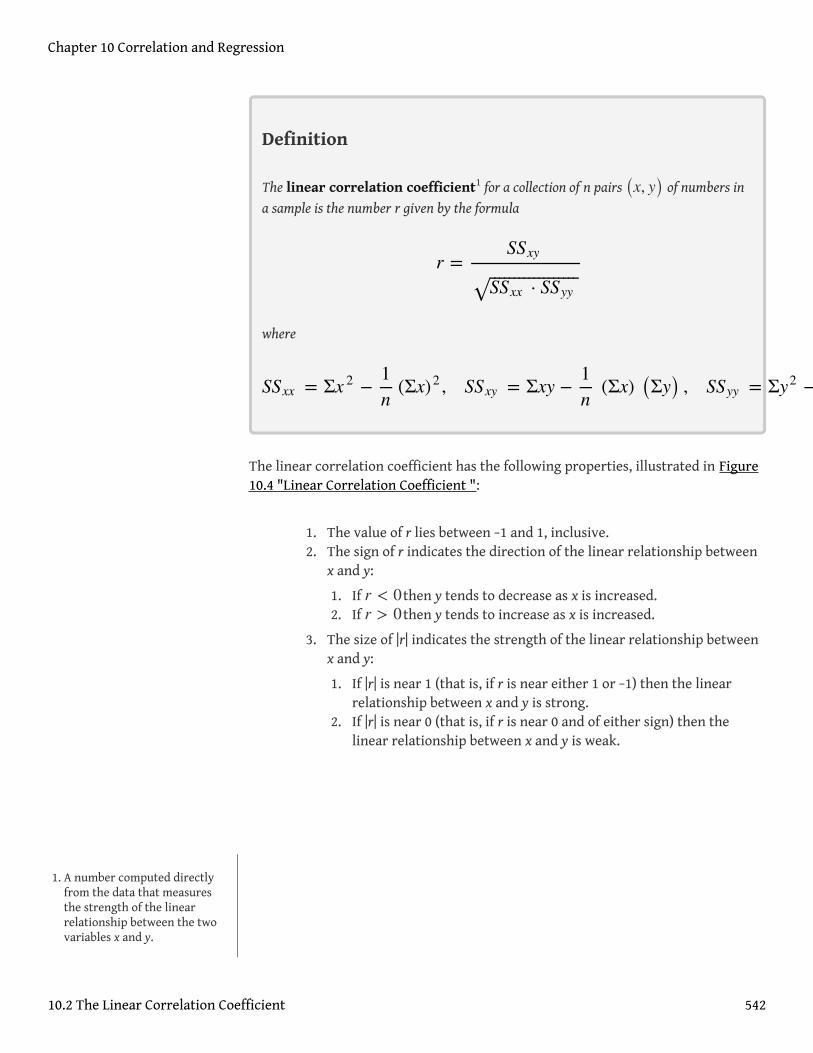
The linear correlation coefficient1 for a collection of n pairs (x, y) of numbers ina sample is the number r given by the formula
where
The linear correlation coefficient has the following properties, illustrated in Figure10.4 "Linear Correlation Coefficient ":
1. The value of r lies between −1 and 1, inclusive.2. The sign of r indicates the direction of the linear relationship between
x and y:
1. If r < 0then y tends to decrease as x is increased.2. If r > 0then y tends to increase as x is increased.
3. The size of |r| indicates the strength of the linear relationship betweenx and y:
1. If |r| is near 1 (that is, if r is near either 1 or −1) then the linearrelationship between x and y is strong.
2. If |r| is near 0 (that is, if r is near 0 and of either sign) then thelinear relationship between x and y is weak.
r =SSxy
SSxx · SSyy⎯ ⎯⎯⎯⎯⎯⎯⎯⎯⎯⎯⎯⎯⎯⎯⎯⎯⎯
√
SSxx = Σx 2 −1n
(Σx)2 , SSxy = Σxy −1n
(Σx) (Σy) , SSyy = Σy2 −1n (Σy) 2
1. A number computed directlyfrom the data that measuresthe strength of the linearrelationship between the twovariables x and y.
Chapter 10 Correlation and Regression
10.2 The Linear Correlation Coefficient 542
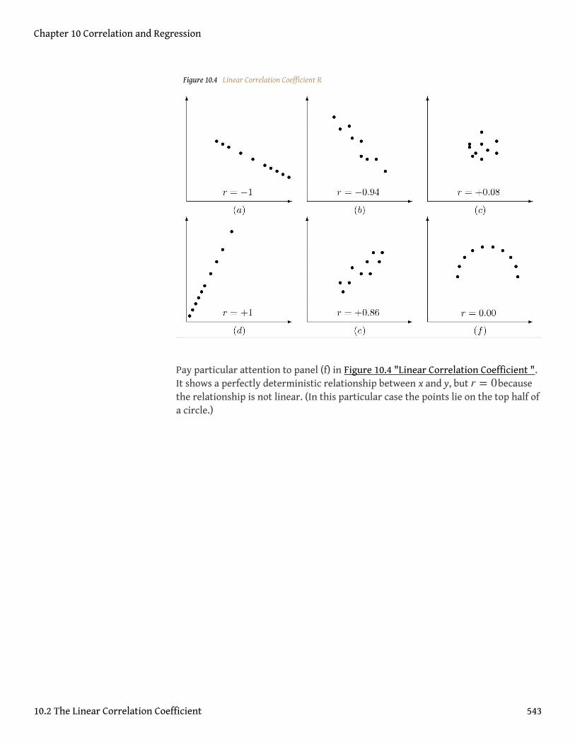
Figure 10.4 Linear Correlation Coefficient R
Pay particular attention to panel (f) in Figure 10.4 "Linear Correlation Coefficient ".It shows a perfectly deterministic relationship between x and y, but r = 0becausethe relationship is not linear. (In this particular case the points lie on the top half ofa circle.)
Chapter 10 Correlation and Regression
10.2 The Linear Correlation Coefficient 543
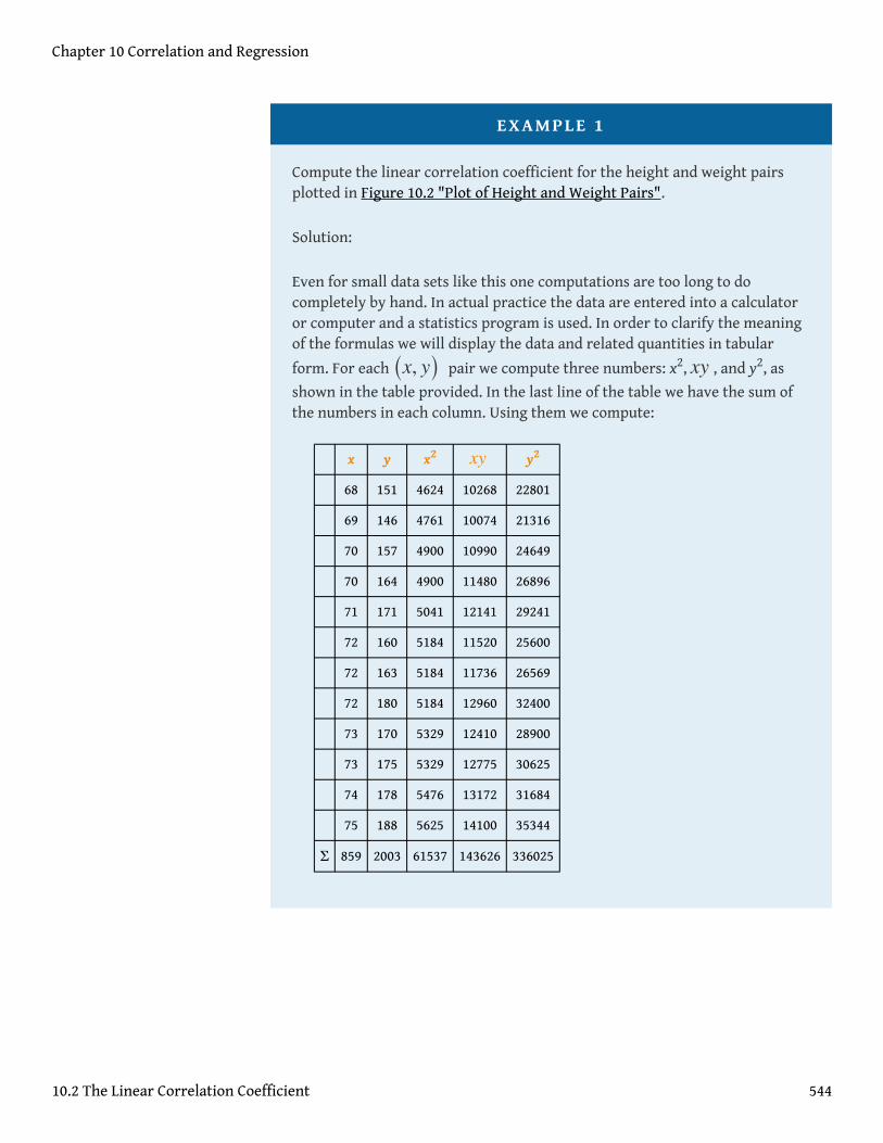
EXAMPLE 1
Compute the linear correlation coefficient for the height and weight pairsplotted in Figure 10.2 "Plot of Height and Weight Pairs".
Solution:
Even for small data sets like this one computations are too long to docompletely by hand. In actual practice the data are entered into a calculatoror computer and a statistics program is used. In order to clarify the meaningof the formulas we will display the data and related quantities in tabular
form. For each (x, y) pair we compute three numbers: x2, xy , and y2, as
shown in the table provided. In the last line of the table we have the sum ofthe numbers in each column. Using them we compute:
x y x2 xy y2
68 151 4624 10268 22801
69 146 4761 10074 21316
70 157 4900 10990 24649
70 164 4900 11480 26896
71 171 5041 12141 29241
72 160 5184 11520 25600
72 163 5184 11736 26569
72 180 5184 12960 32400
73 170 5329 12410 28900
73 175 5329 12775 30625
74 178 5476 13172 31684
75 188 5625 14100 35344
Σ 859 2003 61537 143626 336025
Chapter 10 Correlation and Regression
10.2 The Linear Correlation Coefficient 544
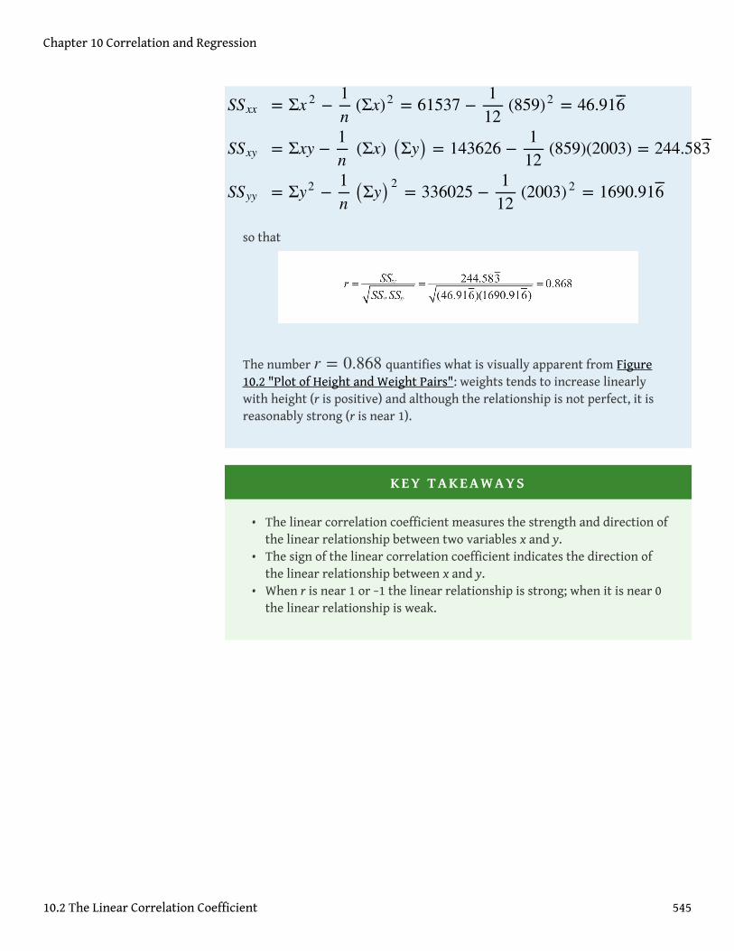
so that
The number r = 0.868 quantifies what is visually apparent from Figure10.2 "Plot of Height and Weight Pairs": weights tends to increase linearlywith height (r is positive) and although the relationship is not perfect, it isreasonably strong (r is near 1).
KEY TAKEAWAYS
• The linear correlation coefficient measures the strength and direction ofthe linear relationship between two variables x and y.
• The sign of the linear correlation coefficient indicates the direction ofthe linear relationship between x and y.
• When r is near 1 or −1 the linear relationship is strong; when it is near 0the linear relationship is weak.
SSxx
SSxy
SSyy
= Σx 2 −1n
(Σx)2 = 61537 −112
(859)2 = 46.916⎯⎯
= Σxy −1n
(Σx) (Σy) = 143626 −112
(859)(2003) = 244.583⎯⎯
= Σy2 −1n (Σy) 2 = 336025 −
112
(2003) 2 = 1690.916⎯⎯
Chapter 10 Correlation and Regression
10.2 The Linear Correlation Coefficient 545
EXERCISES
BASIC
With the exception of the exercises at the end of Section 10.3 "ModellingLinear Relationships with Randomness Present", the first Basic exercise ineach of the following sections through Section 10.7 "Estimation andPrediction" uses the data from the first exercise here, the second Basicexercise uses the data from the second exercise here, and so on, andsimilarly for the Application exercises. Save your computations done onthese exercises so that you do not need to repeat them later.
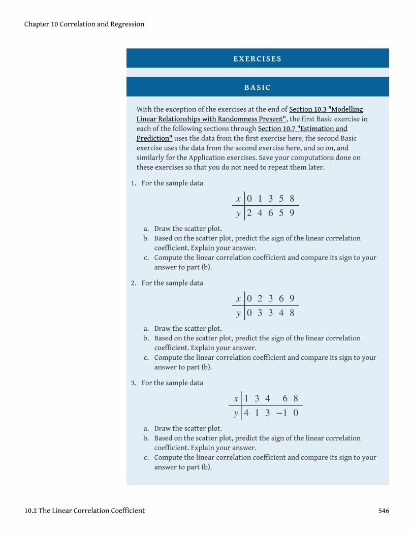
1. For the sample data
a. Draw the scatter plot.b. Based on the scatter plot, predict the sign of the linear correlation
coefficient. Explain your answer.c. Compute the linear correlation coefficient and compare its sign to your
answer to part (b).
2. For the sample data
a. Draw the scatter plot.b. Based on the scatter plot, predict the sign of the linear correlation
coefficient. Explain your answer.c. Compute the linear correlation coefficient and compare its sign to your
answer to part (b).
3. For the sample data
a. Draw the scatter plot.b. Based on the scatter plot, predict the sign of the linear correlation
coefficient. Explain your answer.c. Compute the linear correlation coefficient and compare its sign to your
answer to part (b).
x
y
02
14
36
55
89
x
y
00
23
33
64
98
x
y
14
31
43
6−1
80
Chapter 10 Correlation and Regression
10.2 The Linear Correlation Coefficient 546

4. For the sample data
a. Draw the scatter plot.b. Based on the scatter plot, predict the sign of the linear correlation
coefficient. Explain your answer.c. Compute the linear correlation coefficient and compare its sign to your
answer to part (b).
5. For the sample data
a. Draw the scatter plot.b. Based on the scatter plot, predict the sign of the linear correlation
coefficient. Explain your answer.c. Compute the linear correlation coefficient and compare its sign to your
answer to part (b).
6. For the sample data
a. Draw the scatter plot.b. Based on the scatter plot, predict the sign of the linear correlation
coefficient. Explain your answer.c. Compute the linear correlation coefficient and compare its sign to your
answer to part (b).
7. Compute the linear correlation coefficient for the sample data summarized bythe following information:
8. Compute the linear correlation coefficient for the sample data summarized bythe following information:
x
y
15
25
46
7−3
90
x
y
12
11
35
43
54
x
y
15
3−2
52
5−1
8−3
n = 5
Σ y = 24
Σ x = 25
Σ y2 = 1341 ≤ x ≤ 9
Σ x 2 = 165
Σ xy = 144
Chapter 10 Correlation and Regression
10.2 The Linear Correlation Coefficient 547
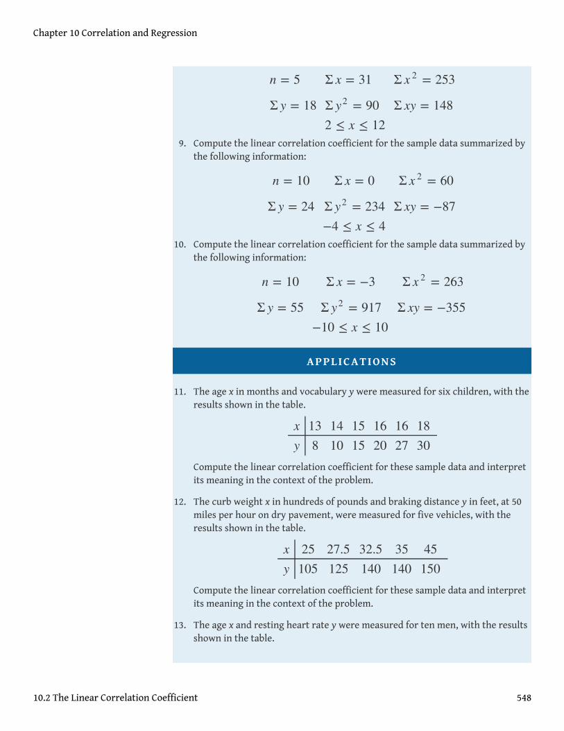
9. Compute the linear correlation coefficient for the sample data summarized bythe following information:
10. Compute the linear correlation coefficient for the sample data summarized bythe following information:
APPLICATIONS
11. The age x in months and vocabulary y were measured for six children, with theresults shown in the table.
Compute the linear correlation coefficient for these sample data and interpretits meaning in the context of the problem.
12. The curb weight x in hundreds of pounds and braking distance y in feet, at 50miles per hour on dry pavement, were measured for five vehicles, with theresults shown in the table.
Compute the linear correlation coefficient for these sample data and interpretits meaning in the context of the problem.
13. The age x and resting heart rate y were measured for ten men, with the resultsshown in the table.
n = 5
Σ y = 18
Σ x = 31
Σ y2 = 902 ≤ x ≤ 12
Σ x 2 = 253
Σ xy = 148
n = 10
Σ y = 24
Σ x = 0
Σ y2 = 234−4 ≤ x ≤ 4
Σ x 2 = 60
Σ xy = −87
n = 10
Σ y = 55
Σ x = −3
Σ y2 = 917−10 ≤ x ≤ 10
Σ x 2 = 263
Σ xy = −355
x
y
138
1410
1515
1620
1627
1830
x
y
25105
27.5125
32.5140
35140
45150
Chapter 10 Correlation and Regression
10.2 The Linear Correlation Coefficient 548

Compute the linear correlation coefficient for these sample data and interpretits meaning in the context of the problem.
14. The wind speed x in miles per hour and wave height y in feet were measuredunder various conditions on an enclosed deep water sea, with the resultsshown in the table,
Compute the linear correlation coefficient for these sample data and interpretits meaning in the context of the problem.
15. The advertising expenditure x and sales y in thousands of dollars for a smallretail business in its first eight years in operation are shown in the table.
Compute the linear correlation coefficient for these sample data and interpretits meaning in the context of the problem.
16. The height x at age 2 and y at age 20, both in inches, for ten women aretabulated in the table.
Compute the linear correlation coefficient for these sample data and interpretits meaning in the context of the problem.
x
y
2072
2371
3073
3774
3574
x
y
4573
5172
5579
6075
6377
x
y
02.0
00.0
20.3
70.7
73.3
x
y
94.9
134.9
203.0
226.9
315.9
x
y
1.4180
1.6184
1.6190
2.0220
x
y
2.0186
2.2215
2.4205
2.6240
x
y
31.360.7
31.761.0
32.563.1
33.564.2
34.465.9
x
y
35.268.2
35.867.6
32.762.3
33.664.9
34.866.8
Chapter 10 Correlation and Regression
10.2 The Linear Correlation Coefficient 549
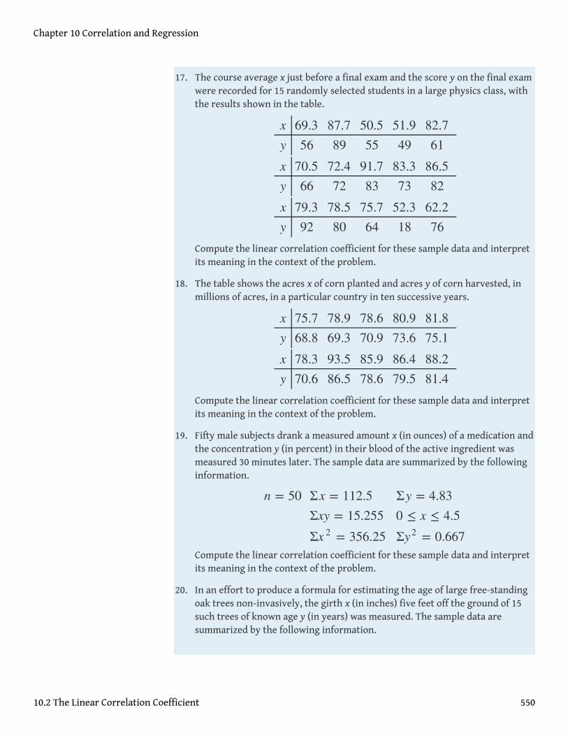
17. The course average x just before a final exam and the score y on the final examwere recorded for 15 randomly selected students in a large physics class, withthe results shown in the table.
Compute the linear correlation coefficient for these sample data and interpretits meaning in the context of the problem.
18. The table shows the acres x of corn planted and acres y of corn harvested, inmillions of acres, in a particular country in ten successive years.
Compute the linear correlation coefficient for these sample data and interpretits meaning in the context of the problem.
19. Fifty male subjects drank a measured amount x (in ounces) of a medication andthe concentration y (in percent) in their blood of the active ingredient wasmeasured 30 minutes later. The sample data are summarized by the followinginformation.
Compute the linear correlation coefficient for these sample data and interpretits meaning in the context of the problem.
20. In an effort to produce a formula for estimating the age of large free-standingoak trees non-invasively, the girth x (in inches) five feet off the ground of 15such trees of known age y (in years) was measured. The sample data aresummarized by the following information.
x
y
69.356
87.789
50.555
51.949
82.761
x
y
70.566
72.472
91.783
83.373
86.582
x
y
79.392
78.580
75.764
52.318
62.276
x
y
75.768.8
78.969.3
78.670.9
80.973.6
81.875.1
x
y
78.370.6
93.586.5
85.978.6
86.479.5
88.281.4
n = 50 Σx = 112.5Σxy = 15.255Σx 2 = 356.25
Σy = 4.830 ≤ x ≤ 4.5Σy2 = 0.667
Chapter 10 Correlation and Regression
10.2 The Linear Correlation Coefficient 550
Compute the linear correlation coefficient for these sample data and interpretits meaning in the context of the problem.
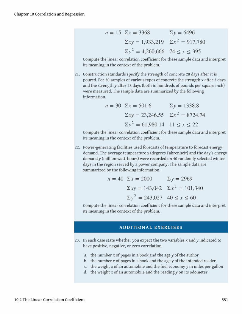
21. Construction standards specify the strength of concrete 28 days after it ispoured. For 30 samples of various types of concrete the strength x after 3 daysand the strength y after 28 days (both in hundreds of pounds per square inch)were measured. The sample data are summarized by the followinginformation.
Compute the linear correlation coefficient for these sample data and interpretits meaning in the context of the problem.
22. Power-generating facilities used forecasts of temperature to forecast energydemand. The average temperature x (degrees Fahrenheit) and the day’s energydemand y (million watt-hours) were recorded on 40 randomly selected winterdays in the region served by a power company. The sample data aresummarized by the following information.
Compute the linear correlation coefficient for these sample data and interpretits meaning in the context of the problem.
ADDITIONAL EXERCISES
23. In each case state whether you expect the two variables x and y indicated tohave positive, negative, or zero correlation.
a. the number x of pages in a book and the age y of the authorb. the number x of pages in a book and the age y of the intended readerc. the weight x of an automobile and the fuel economy y in miles per gallond. the weight x of an automobile and the reading y on its odometer
n = 15 Σx = 3368
Σxy = 1,933,219
Σy2 = 4,260,666
Σy = 6496
Σx 2 = 917,780
74 ≤ x ≤ 395
n = 30 Σx = 501.6
Σxy = 23,246.55
Σy2 = 61,980.14
Σy = 1338.8
Σx 2 = 8724.74
11 ≤ x ≤ 22
n = 40 Σx = 2000
Σxy = 143,042
Σy2 = 243,027
Σy = 2969
Σx 2 = 101,340
40 ≤ x ≤ 60
Chapter 10 Correlation and Regression
10.2 The Linear Correlation Coefficient 551
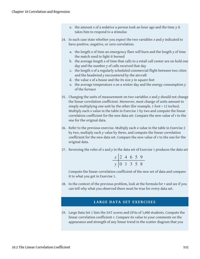
e. the amount x of a sedative a person took an hour ago and the time y ittakes him to respond to a stimulus
24. In each case state whether you expect the two variables x and y indicated tohave positive, negative, or zero correlation.
a. the length x of time an emergency flare will burn and the length y of timethe match used to light it burned
b. the average length x of time that calls to a retail call center are on hold oneday and the number y of calls received that day
c. the length x of a regularly scheduled commercial flight between two citiesand the headwind y encountered by the aircraft
d. the value x of a house and the its size y in square feete. the average temperature x on a winter day and the energy consumption y
of the furnace
25. Changing the units of measurement on two variables x and y should not changethe linear correlation coefficient. Moreover, most change of units amount tosimply multiplying one unit by the other (for example, 1 foot = 12 inches).Multiply each x value in the table in Exercise 1 by two and compute the linearcorrelation coefficient for the new data set. Compare the new value of r to theone for the original data.
26. Refer to the previous exercise. Multiply each x value in the table in Exercise 2by two, multiply each y value by three, and compute the linear correlationcoefficient for the new data set. Compare the new value of r to the one for theoriginal data.
27. Reversing the roles of x and y in the data set of Exercise 1 produces the data set
Compute the linear correlation coefficient of the new set of data and compareit to what you got in Exercise 1.
28. In the context of the previous problem, look at the formula for r and see if youcan tell why what you observed there must be true for every data set.
LARGE DATA SET EXERCISES
29. Large Data Set 1 lists the SAT scores and GPAs of 1,000 students. Compute thelinear correlation coefficient r. Compare its value to your comments on theappearance and strength of any linear trend in the scatter diagram that you
x
y
20
41
63
55
98
Chapter 10 Correlation and Regression
10.2 The Linear Correlation Coefficient 552
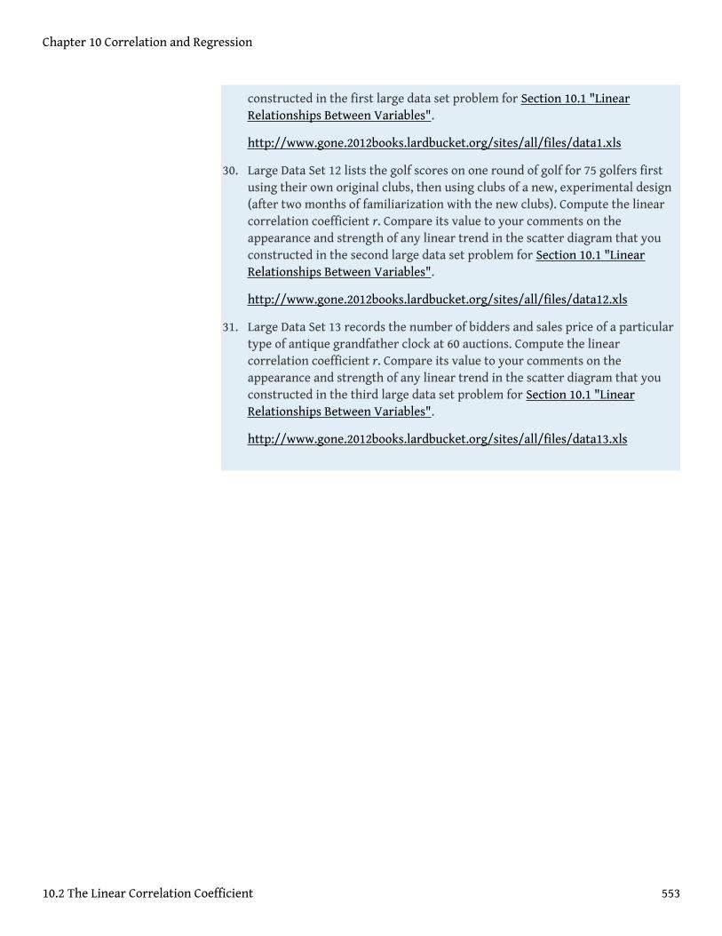
constructed in the first large data set problem for Section 10.1 "LinearRelationships Between Variables".
http://www.gone.2012books.lardbucket.org/sites/all/files/data1.xls
30. Large Data Set 12 lists the golf scores on one round of golf for 75 golfers firstusing their own original clubs, then using clubs of a new, experimental design(after two months of familiarization with the new clubs). Compute the linearcorrelation coefficient r. Compare its value to your comments on theappearance and strength of any linear trend in the scatter diagram that youconstructed in the second large data set problem for Section 10.1 "LinearRelationships Between Variables".
http://www.gone.2012books.lardbucket.org/sites/all/files/data12.xls
31. Large Data Set 13 records the number of bidders and sales price of a particulartype of antique grandfather clock at 60 auctions. Compute the linearcorrelation coefficient r. Compare its value to your comments on theappearance and strength of any linear trend in the scatter diagram that youconstructed in the third large data set problem for Section 10.1 "LinearRelationships Between Variables".
http://www.gone.2012books.lardbucket.org/sites/all/files/data13.xls
Chapter 10 Correlation and Regression
10.2 The Linear Correlation Coefficient 553
ANSWERS
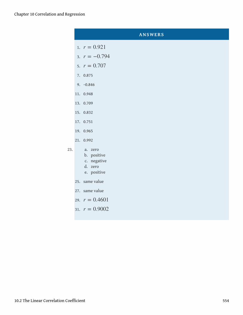
1. r = 0.9213. r = −0.7945. r = 0.7077. 0.875
9. −0.846
11. 0.948
13. 0.709
15. 0.832
17. 0.751
19. 0.965
21. 0.992
23. a. zerob. positivec. negatived. zeroe. positive
25. same value
27. same value
29. r = 0.460131. r = 0.9002
Chapter 10 Correlation and Regression
10.2 The Linear Correlation Coefficient 554
10.3 Modelling Linear Relationships with Randomness Present
LEARNING OBJECTIVE
1. To learn the framework in which the statistical analysis of the linearrelationship between two variables x and y will be done.
In this chapter we are dealing with a population for which we can associate to eachelement two measurements, x and y. We are interested in situations in which thevalue of x can be used to draw conclusions about the value of y, such as predictingthe resale value y of a residential house based on its size x. Since the relationshipbetween x and y is not deterministic, statistical procedures must be applied. For anystatistical procedures, given in this book or elsewhere, the associated formulas arevalid only under specific assumptions. The set of assumptions in simple linearregression are a mathematical description of the relationship between x and y. Sucha set of assumptions is known as a model.
For each fixed value of x a sub-population of the full population is determined, suchas the collection of all houses with 2,100 square feet of living space. For eachelement of that sub-population there is a measurement y, such as the value of any2,100-square-foot house. Let E (y) denote the mean of all the y-values for each
particular value of x. E (y) can change from x-value to x-value, such as the meanvalue of all 2,100-square-foot houses, the (different) mean value for all 2,500-squarefoot-houses, and so on.
Our first assumption is that the relationship between x and the mean of the y-valuesin the sub-population determined by x is linear. This means that there existnumbers β1 and β0 such that
This linear relationship is the reason for the word “linear” in “simple linearregression” below. (The word “simple” means that y depends on only one othervariable and not two or more.)
Our next assumption is that for each value of x the y-values scatter about the meanE (y) according to a normal distribution centered at E (y) and with a standard
deviation σ that is the same for every value of x. This is the same as saying that
E (y) = β1x + β0
Chapter 10 Correlation and Regression
555
there exists a normally distributed random variable ε with mean 0 and standarddeviation σ so that the relationship between x and y in the whole population is
Our last assumption is that the random deviations associated with differentobservations are independent.
In summary, the model is:
Simple Linear Regression Model
For each point (x, y) in data set the y-value is an independent observation of
where β1 and β0 are fixed parameters and ε is a normally distributed randomvariable with mean 0 and an unknown standard deviation σ.
The line with equation y = β1x + β0 is called the population regressionline2.
Figure 10.5 "The Simple Linear Model Concept" illustrates the model. The symbolsN (μ, σ 2)denote a normal distribution with mean μ and variance σ 2 , hence
standard deviation σ.
y = β1x + β0 + ε
y = β1x + β0 + ε
2. The line with equationy = β1x + β0 that gives themean of the variable y over thesub-population determined byx.
Chapter 10 Correlation and Regression
10.3 Modelling Linear Relationships with Randomness Present 556
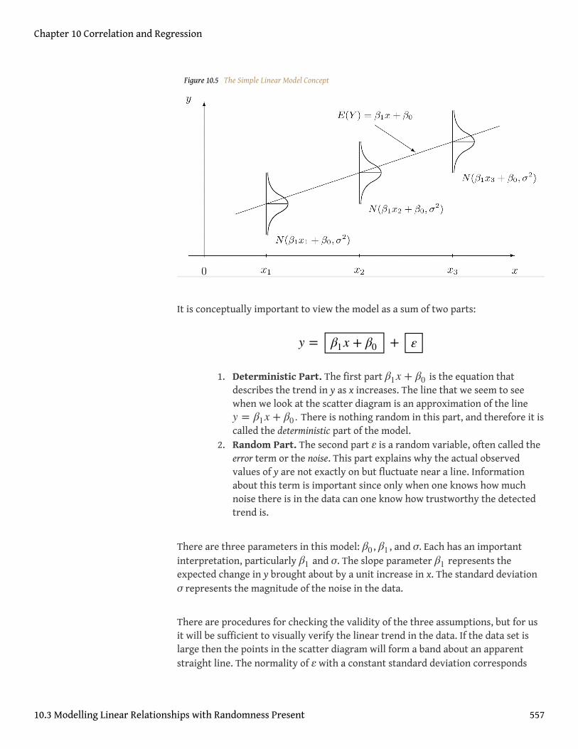
Figure 10.5 The Simple Linear Model Concept
It is conceptually important to view the model as a sum of two parts:
1. Deterministic Part. The first part β1x + β0 is the equation thatdescribes the trend in y as x increases. The line that we seem to seewhen we look at the scatter diagram is an approximation of the liney = β1x + β0 . There is nothing random in this part, and therefore it iscalled the deterministic part of the model.
2. Random Part. The second part ε is a random variable, often called theerror term or the noise. This part explains why the actual observedvalues of y are not exactly on but fluctuate near a line. Informationabout this term is important since only when one knows how muchnoise there is in the data can one know how trustworthy the detectedtrend is.
There are three parameters in this model: β0 , β1 , and σ. Each has an importantinterpretation, particularly β1 and σ. The slope parameter β1 represents theexpected change in y brought about by a unit increase in x. The standard deviationσ represents the magnitude of the noise in the data.
There are procedures for checking the validity of the three assumptions, but for usit will be sufficient to visually verify the linear trend in the data. If the data set islarge then the points in the scatter diagram will form a band about an apparentstraight line. The normality of ε with a constant standard deviation corresponds
y = β1x + β0 + ε
Chapter 10 Correlation and Regression
10.3 Modelling Linear Relationships with Randomness Present 557
graphically to the band being of roughly constant width, and with most pointsconcentrated near the middle of the band.
Fortunately, the three assumptions do not need to hold exactly in order for theprocedures and analysis developed in this chapter to be useful.
KEY TAKEAWAY
• Statistical procedures are valid only when certain assumptions are valid.The assumptions underlying the analyses done in this chapter aregraphically summarized in Figure 10.5 "The Simple Linear ModelConcept".
EXERCISES
1. State the three assumptions that are the basis for the Simple Linear RegressionModel.
2. The Simple Linear Regression Model is summarized by the equation
Identify the deterministic part and the random part.
3. Is the number β1 in the equation y = β1x + β0 a statistic or a populationparameter? Explain.
4. Is the number σ in the Simple Linear Regression Model a statistic or apopulation parameter? Explain.
5. Describe what to look for in a scatter diagram in order to check that theassumptions of the Simple Linear Regression Model are true.
6. True or false: the assumptions of the Simple Linear Regression Model musthold exactly in order for the procedures and analysis developed in this chapterto be useful.
y = β1x + β0 + ε
Chapter 10 Correlation and Regression
10.3 Modelling Linear Relationships with Randomness Present 558

ANSWERS
1. a. The mean of y is linearly related to x.b. For each given x, y is a normal random variable with mean β1x + β0 and
standard deviation σ.c. All the observations of y in the sample are independent.
3. β1 is a population parameter.
5. A linear trend.
Chapter 10 Correlation and Regression
10.3 Modelling Linear Relationships with Randomness Present 559
10.4 The Least Squares Regression Line
LEARNING OBJECTIVES
1. To learn how to measure how well a straight line fits a collection of data.2. To learn how to construct the least squares regression line, the straight
line that best fits a collection of data.3. To learn the meaning of the slope of the least squares regression line.4. To learn how to use the least squares regression line to estimate the
response variable y in terms of the predictor variable x.
Goodness of Fit of a Straight Line to Data
Once the scatter diagram of the data has been drawn and the model assumptionsdescribed in the previous sections at least visually verified (and perhaps thecorrelation coefficient r computed to quantitatively verify the linear trend), thenext step in the analysis is to find the straight line that best fits the data. We willexplain how to measure how well a straight line fits a collection of points by
examining how well the line y = 12 x−1 fits the data set
(which will be used as a running example for the next three sections). We will write
the equation of this line as y = 12 x−1with an accent on the y to indicate that the
y-values computed using this equation are not from the data. We will do this with
all lines approximating data sets. The line y = 12 x−1was selected as one that
seems to fit the data reasonably well.
The idea for measuring the goodness of fit of a straight line to data is illustrated inFigure 10.6 "Plot of the Five-Point Data and the Line ", in which the graph of the
line y = 12 x−1has been superimposed on the scatter plot for the sample data set.
x
y
20
21
62
83
103
Chapter 10 Correlation and Regression
560

Figure 10.6 Plot of the Five-Point Data and the Line y = 12 x−1
To each point in the data set there is associated an “error3,” the positive ornegative vertical distance from the point to the line: positive if the point is abovethe line and negative if it is below the line. The error can be computed as the actualy-value of the point minus the y-value y that is “predicted” by inserting the x-valueof the data point into the formula for the line:
The computation of the error for each of the five points in the data set is shown inTable 10.1 "The Errors in Fitting Data with a Straight Line".
Table 10.1 The Errors in Fitting Data with a Straight Line
x y y = 12 x−1 y − y (y − y)2
2 0 0 0 0
2 1 0 1 1
error at data point (x, y) = (true y) − (predicted y) = y − y
3. Using y − y , the actual y-value of a data point minus they-value that is computed fromthe equation of the line fittingthe data.
Chapter 10 Correlation and Regression
10.4 The Least Squares Regression Line 561

x y y = 12 x−1 y − y (y − y)2
6 2 2 0 0
8 3 3 0 0
10 3 4 −1 1
Σ - - - 0 2
A first thought for a measure of the goodness of fit of the line to the data would besimply to add the errors at every point, but the example shows that this cannotwork well in general. The line does not fit the data perfectly (no line can), yetbecause of cancellation of positive and negative errors the sum of the errors (thefourth column of numbers) is zero. Instead goodness of fit is measured by the sumof the squares of the errors. Squaring eliminates the minus signs, so no cancellationcan occur. For the data and line in Figure 10.6 "Plot of the Five-Point Data and theLine " the sum of the squared errors (the last column of numbers) is 2. This numbermeasures the goodness of fit of the line to the data.
Definition
The goodness of fit of a line y = mx + b to a set of n pairs (x, y) of numbers in asample is the sum of the squared errors
(n terms in the sum, one for each data pair).
The Least Squares Regression Line
Given any collection of pairs of numbers (except when all the x-values are the same)and the corresponding scatter diagram, there always exists exactly one straight linethat fits the data better than any other, in the sense of minimizing the sum of thesquared errors. It is called the least squares regression line. Moreover there areformulas for its slope and y-intercept.
Σ(y − y)2
Chapter 10 Correlation and Regression
10.4 The Least Squares Regression Line 562
Definition
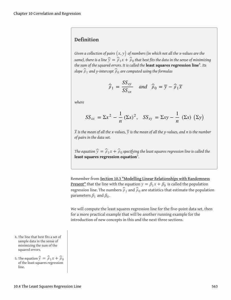
Given a collection of pairs (x, y) of numbers (in which not all the x-values are the
same), there is a line y = β 1x + β 0 that best fits the data in the sense of minimizingthe sum of the squared errors. It is called the least squares regression line4. Itsslope β 1 and y-intercept β 0 are computed using the formulas
where
x⎯⎯ is the mean of all the x-values, y⎯⎯ is the mean of all the y-values, and n is the numberof pairs in the data set.
The equation y = β 1x + β 0 specifying the least squares regression line is called theleast squares regression equation5.
Remember from Section 10.3 "Modelling Linear Relationships with RandomnessPresent" that the line with the equation y = β1x + β0 is called the populationregression line. The numbers β 1 and β 0 are statistics that estimate the populationparameters β1 and β0 .
We will compute the least squares regression line for the five-point data set, thenfor a more practical example that will be another running example for theintroduction of new concepts in this and the next three sections.
β 1 =SSxy
SSxxand β 0 = y⎯⎯ − β 1x
⎯⎯
SSxx = Σx 2 −1n
(Σx)2 , SSxy = Σxy −1n
(Σx) (Σy)
4. The line that best fits a set ofsample data in the sense ofminimizing the sum of thesquared errors.
5. The equation y = β 1x + β 0of the least squares regressionline.
Chapter 10 Correlation and Regression
10.4 The Least Squares Regression Line 563
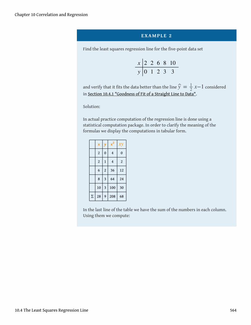
EXAMPLE 2
Find the least squares regression line for the five-point data set
and verify that it fits the data better than the line y = 12 x−1 considered
in Section 10.4.1 "Goodness of Fit of a Straight Line to Data".
Solution:
In actual practice computation of the regression line is done using astatistical computation package. In order to clarify the meaning of theformulas we display the computations in tabular form.
x y x2 xy
2 0 4 0
2 1 4 2
6 2 36 12
8 3 64 24
10 3 100 30
Σ 28 9 208 68
In the last line of the table we have the sum of the numbers in each column.Using them we compute:
x
y
20
21
62
83
103
Chapter 10 Correlation and Regression
10.4 The Least Squares Regression Line 564
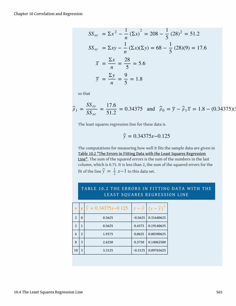
so that
The least squares regression line for these data is
The computations for measuring how well it fits the sample data are given inTable 10.2 "The Errors in Fitting Data with the Least Squares RegressionLine". The sum of the squared errors is the sum of the numbers in the lastcolumn, which is 0.75. It is less than 2, the sum of the squared errors for the
fit of the line y = 12 x−1 to this data set.
T A B L E 1 0 . 2 T H E E R R O R S I N F I T T I N G D A T A W I T H T H EL E A S T S Q U A R E S R E G R E S S I O N L I N E
x y y = 0.34375x−0.125 y − y (y − y)22 0 0.5625 −0.5625 0.31640625
2 1 0.5625 0.4375 0.19140625
6 2 1.9375 0.0625 0.00390625
8 3 2.6250 0.3750 0.14062500
10 3 3.3125 −0.3125 0.09765625
SSxx
SSxy
x⎯⎯
y⎯⎯
= Σx 2 −1n
(Σx)2= 208 −
15
(28)2 = 51.2
= Σxy −1n
(Σx)(Σy) = 68 −15
(28)(9) = 17.6
=Σxn
=285
= 5.6
=Σyn
=95
= 1.8
β 1 =SSxy
SSxx=
17.651.2
= 0.34375 and β 0 = y⎯⎯ − β 1x⎯⎯ = 1.8 − (0.34375)(5.6) = −0.125
y = 0.34375x−0.125
Chapter 10 Correlation and Regression
10.4 The Least Squares Regression Line 565
EXAMPLE 3
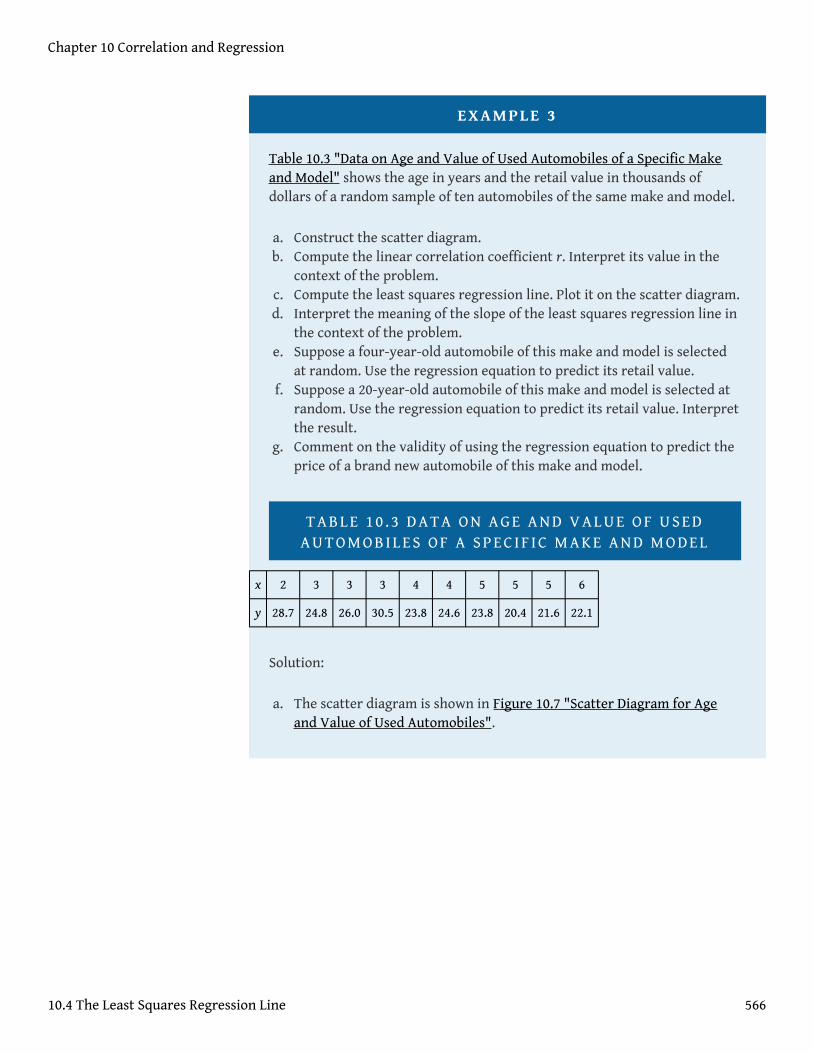
Table 10.3 "Data on Age and Value of Used Automobiles of a Specific Makeand Model" shows the age in years and the retail value in thousands ofdollars of a random sample of ten automobiles of the same make and model.
a. Construct the scatter diagram.b. Compute the linear correlation coefficient r. Interpret its value in the
context of the problem.c. Compute the least squares regression line. Plot it on the scatter diagram.d. Interpret the meaning of the slope of the least squares regression line in
the context of the problem.e. Suppose a four-year-old automobile of this make and model is selected
at random. Use the regression equation to predict its retail value.f. Suppose a 20-year-old automobile of this make and model is selected at
random. Use the regression equation to predict its retail value. Interpretthe result.
g. Comment on the validity of using the regression equation to predict theprice of a brand new automobile of this make and model.
T A B L E 1 0 . 3 D A T A O N A G E A N D V A L U E O F U S E DA U T O M O B I L E S O F A S P E C I F I C M A K E A N D M O D E L
x 2 3 3 3 4 4 5 5 5 6
y 28.7 24.8 26.0 30.5 23.8 24.6 23.8 20.4 21.6 22.1
Solution:
a. The scatter diagram is shown in Figure 10.7 "Scatter Diagram for Ageand Value of Used Automobiles".
Chapter 10 Correlation and Regression
10.4 The Least Squares Regression Line 566
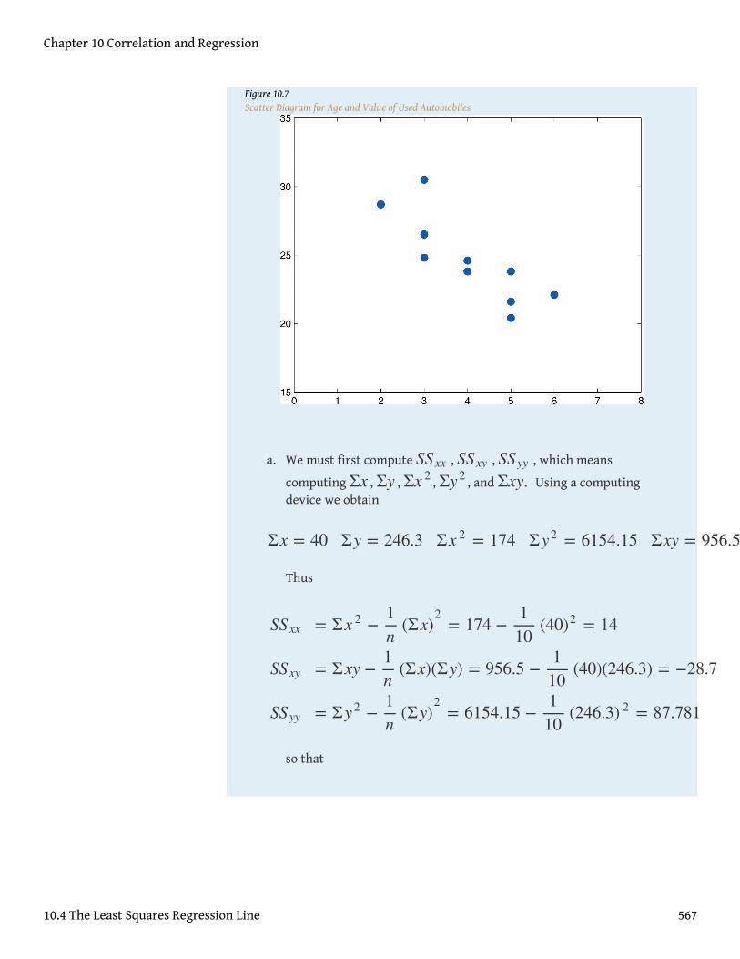
Figure 10.7Scatter Diagram for Age and Value of Used Automobiles
a. We must first compute SSxx , SSxy , SSyy , which means
computing Σx , Σy , Σx 2 , Σy2 , and Σxy. Using a computingdevice we obtain
Thus
so that
Σx = 40 Σy = 246.3 Σx 2 = 174 Σy2 = 6154.15 Σxy = 956.5
SSxx
SSxy
SSyy
= Σx 2 −1n
(Σx)2= 174 −
110
(40)2 = 14
= Σxy −1n
(Σx)(Σy) = 956.5 −110
(40)(246.3) = −28.7
= Σy2 −1n
(Σy)2= 6154.15 −
110
(246.3) 2 = 87.781
Chapter 10 Correlation and Regression
10.4 The Least Squares Regression Line 567
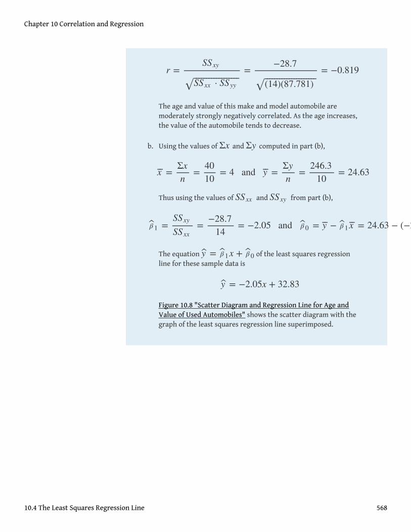
The age and value of this make and model automobile aremoderately strongly negatively correlated. As the age increases,the value of the automobile tends to decrease.
b. Using the values of Σx and Σy computed in part (b),
Thus using the values of SSxx and SSxy from part (b),
The equation y = β 1x + β 0 of the least squares regressionline for these sample data is
Figure 10.8 "Scatter Diagram and Regression Line for Age andValue of Used Automobiles" shows the scatter diagram with thegraph of the least squares regression line superimposed.
r =SSxy
SSxx · SSyy⎯ ⎯⎯⎯⎯⎯⎯⎯⎯⎯⎯⎯⎯⎯⎯⎯⎯⎯
√=
−28.7
(14)(87.781)⎯ ⎯⎯⎯⎯⎯⎯⎯⎯⎯⎯⎯⎯⎯⎯⎯⎯⎯⎯⎯⎯√
= −0.819
x⎯⎯ =Σxn
=4010
= 4 and y⎯⎯ =Σyn
=246.310
= 24.63
β 1 =SSxy
SSxx=
−28.714
= −2.05 and β 0 = y⎯⎯ − β 1x⎯⎯ = 24.63 − (−2.05)(4) = 32.83
y = −2.05x + 32.83
Chapter 10 Correlation and Regression
10.4 The Least Squares Regression Line 568
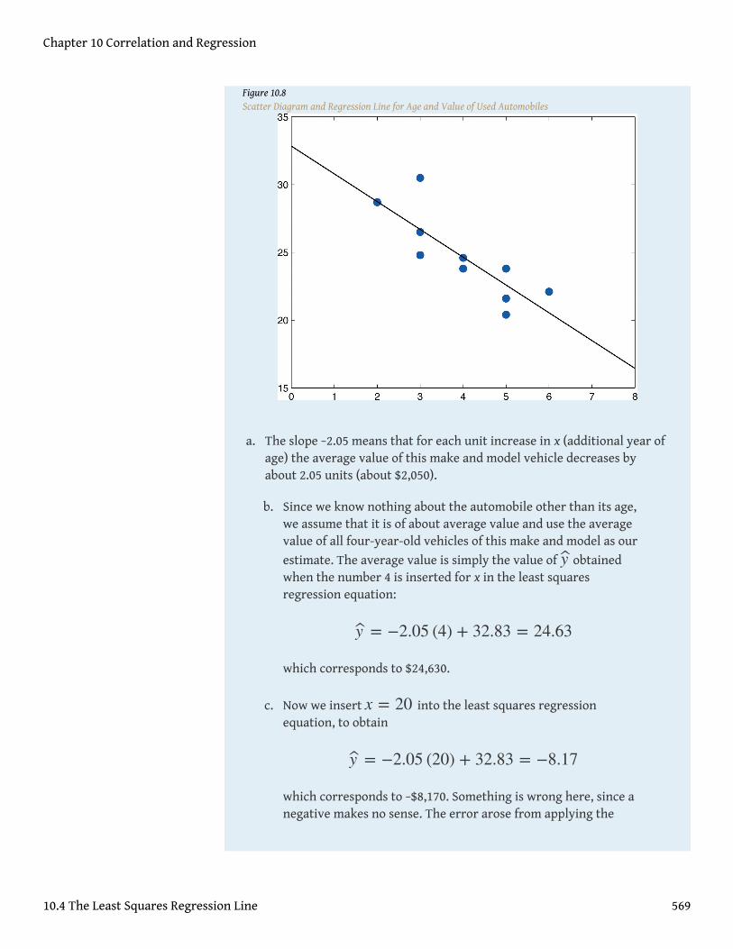
Figure 10.8Scatter Diagram and Regression Line for Age and Value of Used Automobiles
a. The slope −2.05 means that for each unit increase in x (additional year ofage) the average value of this make and model vehicle decreases byabout 2.05 units (about $2,050).
b. Since we know nothing about the automobile other than its age,we assume that it is of about average value and use the averagevalue of all four-year-old vehicles of this make and model as our
estimate. The average value is simply the value of y obtainedwhen the number 4 is inserted for x in the least squaresregression equation:
which corresponds to $24,630.
c. Now we insert x = 20 into the least squares regressionequation, to obtain
which corresponds to −$8,170. Something is wrong here, since anegative makes no sense. The error arose from applying the
y = −2.05 (4) + 32.83 = 24.63
y = −2.05 (20) + 32.83 = −8.17
Chapter 10 Correlation and Regression
10.4 The Least Squares Regression Line 569
regression equation to a value of x not in the range of x-values inthe original data, from two to six years.
Applying the regression equation y = β 1x + β 0 to a value of xoutside the range of x-values in the data set is called extrapolation.It is an invalid use of the regression equation and should beavoided.
d. The price of a brand new vehicle of this make and model is the value ofthe automobile at age 0. If the value x = 0 is inserted into the
regression equation the result is always β 0 , the y-intercept, in this case32.83, which corresponds to $32,830. But this is a case of extrapolation,just as part (f) was, hence this result is invalid, although not obviouslyso. In the context of the problem, since automobiles tend to lose valuemuch more quickly immediately after they are purchased than they doafter they are several years old, the number $32,830 is probably anunderestimate of the price of a new automobile of this make and model.
For emphasis we highlight the points raised by parts (f) and (g) of the example.
Definition
The process of using the least squares regression equation to estimate the value of y at avalue of x that does not lie in the range of the x-values in the data set that was used toform the regression line is called extrapolation6. It is an invalid use of the regressionequation that can lead to errors, hence should be avoided.
The Sum of the Squared Errors SSE
In general, in order to measure the goodness of fit of a line to a set of data, we mustcompute the predicted y-value y at every point in the data set, compute each error,square it, and then add up all the squares. In the case of the least squares regressionline, however, the line that best fits the data, the sum of the squared errors can becomputed directly from the data using the following formula.
6. The process of using the leastsquares regression equation toestimate the value of y at an xvalue not in the proper range.
Chapter 10 Correlation and Regression
10.4 The Least Squares Regression Line 570
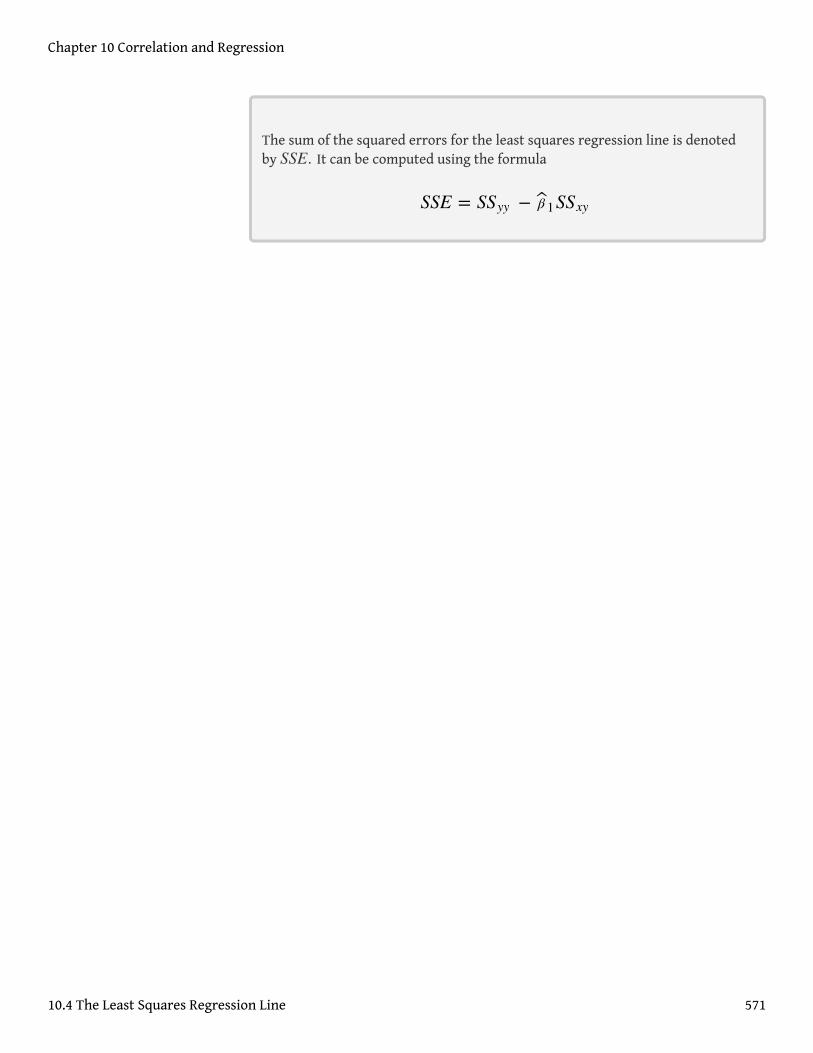
The sum of the squared errors for the least squares regression line is denotedby SSE. It can be computed using the formula
SSE = SSyy − β 1SSxy
Chapter 10 Correlation and Regression
10.4 The Least Squares Regression Line 571
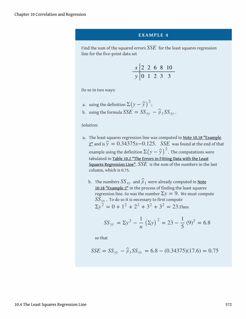
EXAMPLE 4
Find the sum of the squared errors SSE for the least squares regressionline for the five-point data set
Do so in two ways:
a. using the definition Σ(y − y)2 ;
b. using the formula SSE = SSyy − β 1SSxy .
Solution:
a. The least squares regression line was computed in Note 10.18 "Example
2" and is y = 0.34375x−0.125. SSE was found at the end of that
example using the definition Σ(y − y)2 . The computations were
tabulated in Table 10.2 "The Errors in Fitting Data with the LeastSquares Regression Line". SSE is the sum of the numbers in the lastcolumn, which is 0.75.
b. The numbers SSxy and β 1 were already computed in Note10.18 "Example 2" in the process of finding the least squaresregression line. So was the number Σy = 9. We must computeSSyy . To do so it is necessary to first compute
Σy2 = 0 + 12 + 22 + 32 + 32 = 23.Then
so that
x
y
20
21
62
83
103
SSyy = Σy2 −1n (Σy) 2 = 23 −
15
(9)2 = 6.8
SSE = SSyy − β 1SSxy = 6.8 − (0.34375)(17.6) = 0.75
Chapter 10 Correlation and Regression
10.4 The Least Squares Regression Line 572
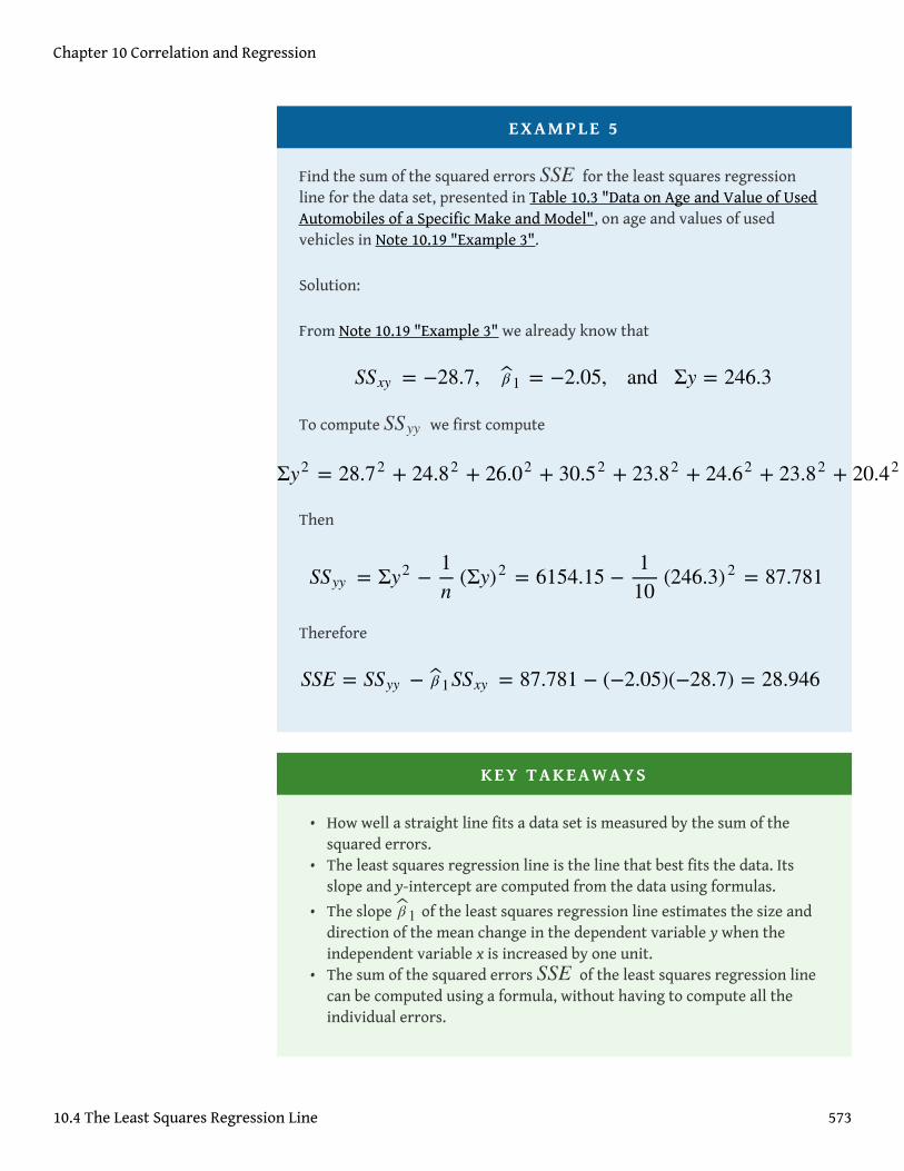
EXAMPLE 5
Find the sum of the squared errors SSE for the least squares regressionline for the data set, presented in Table 10.3 "Data on Age and Value of UsedAutomobiles of a Specific Make and Model", on age and values of usedvehicles in Note 10.19 "Example 3".
Solution:
From Note 10.19 "Example 3" we already know that
To compute SSyy we first compute
Then
Therefore
KEY TAKEAWAYS
• How well a straight line fits a data set is measured by the sum of thesquared errors.
• The least squares regression line is the line that best fits the data. Itsslope and y-intercept are computed from the data using formulas.
• The slope β 1 of the least squares regression line estimates the size anddirection of the mean change in the dependent variable y when theindependent variable x is increased by one unit.
• The sum of the squared errors SSE of the least squares regression linecan be computed using a formula, without having to compute all theindividual errors.
SSxy = −28.7, β 1 = −2.05, and Σy = 246.3
Σy2 = 28.72 + 24.82 + 26.02 + 30.52 + 23.82 + 24.62 + 23.82 + 20.42 + 21.62 + 22.12 = 6154.15
SSyy = Σy2 −1n
(Σy)2 = 6154.15 −110
(246.3) 2 = 87.781
SSE = SSyy − β 1SSxy = 87.781 − (−2.05)(−28.7) = 28.946
Chapter 10 Correlation and Regression
10.4 The Least Squares Regression Line 573
EXERCISES
BASIC
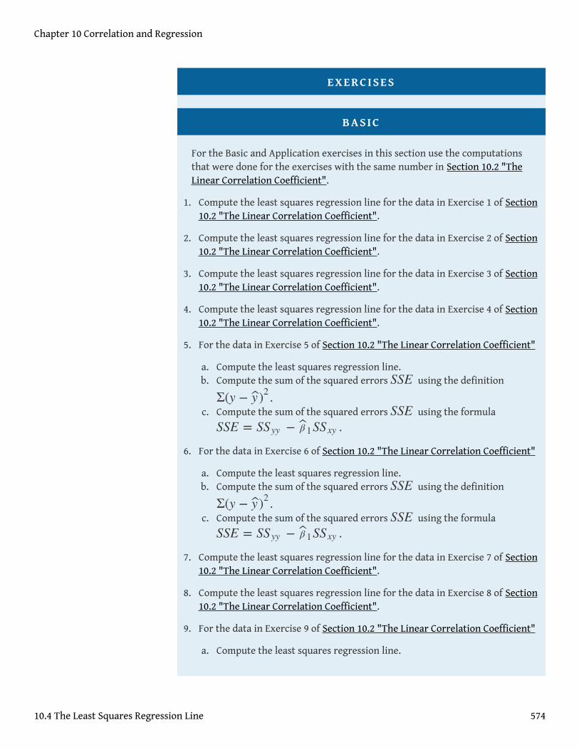
For the Basic and Application exercises in this section use the computationsthat were done for the exercises with the same number in Section 10.2 "TheLinear Correlation Coefficient".
1. Compute the least squares regression line for the data in Exercise 1 of Section10.2 "The Linear Correlation Coefficient".
2. Compute the least squares regression line for the data in Exercise 2 of Section10.2 "The Linear Correlation Coefficient".
3. Compute the least squares regression line for the data in Exercise 3 of Section10.2 "The Linear Correlation Coefficient".
4. Compute the least squares regression line for the data in Exercise 4 of Section10.2 "The Linear Correlation Coefficient".
5. For the data in Exercise 5 of Section 10.2 "The Linear Correlation Coefficient"
a. Compute the least squares regression line.b. Compute the sum of the squared errors SSE using the definition
Σ(y − y )2 .c. Compute the sum of the squared errors SSE using the formula
SSE = SSyy − β 1SSxy .
6. For the data in Exercise 6 of Section 10.2 "The Linear Correlation Coefficient"
a. Compute the least squares regression line.b. Compute the sum of the squared errors SSE using the definition
Σ(y − y )2 .c. Compute the sum of the squared errors SSE using the formula
SSE = SSyy − β 1SSxy .
7. Compute the least squares regression line for the data in Exercise 7 of Section10.2 "The Linear Correlation Coefficient".
8. Compute the least squares regression line for the data in Exercise 8 of Section10.2 "The Linear Correlation Coefficient".
9. For the data in Exercise 9 of Section 10.2 "The Linear Correlation Coefficient"
a. Compute the least squares regression line.
Chapter 10 Correlation and Regression
10.4 The Least Squares Regression Line 574

b. Can you compute the sum of the squared errors SSE using the definition
Σ(y − y )2 ? Explain.c. Compute the sum of the squared errors SSE using the formula
SSE = SSyy − β 1SSxy .
10. For the data in Exercise 10 of Section 10.2 "The Linear Correlation Coefficient"
a. Compute the least squares regression line.b. Can you compute the sum of the squared errors SSE using the definition
Σ(y − y )2 ? Explain.c. Compute the sum of the squared errors SSE using the formula
SSE = SSyy − β 1SSxy .
APPLICATIONS
11. For the data in Exercise 11 of Section 10.2 "The Linear Correlation Coefficient"
a. Compute the least squares regression line.b. On average, how many new words does a child from 13 to 18 months old
learn each month? Explain.c. Estimate the average vocabulary of all 16-month-old children.
12. For the data in Exercise 12 of Section 10.2 "The Linear Correlation Coefficient"
a. Compute the least squares regression line.b. On average, how many additional feet are added to the braking distance
for each additional 100 pounds of weight? Explain.c. Estimate the average braking distance of all cars weighing 3,000 pounds.
13. For the data in Exercise 13 of Section 10.2 "The Linear Correlation Coefficient"
a. Compute the least squares regression line.b. Estimate the average resting heart rate of all 40-year-old men.c. Estimate the average resting heart rate of all newborn baby boys.
Comment on the validity of the estimate.
14. For the data in Exercise 14 of Section 10.2 "The Linear Correlation Coefficient"
a. Compute the least squares regression line.b. Estimate the average wave height when the wind is blowing at 10 miles per
hour.c. Estimate the average wave height when there is no wind blowing.
Comment on the validity of the estimate.
15. For the data in Exercise 15 of Section 10.2 "The Linear Correlation Coefficient"
Chapter 10 Correlation and Regression
10.4 The Least Squares Regression Line 575
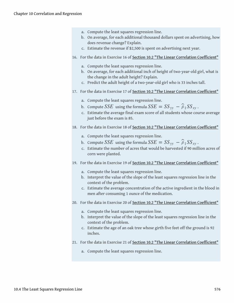
a. Compute the least squares regression line.b. On average, for each additional thousand dollars spent on advertising, how
does revenue change? Explain.c. Estimate the revenue if $2,500 is spent on advertising next year.
16. For the data in Exercise 16 of Section 10.2 "The Linear Correlation Coefficient"
a. Compute the least squares regression line.b. On average, for each additional inch of height of two-year-old girl, what is
the change in the adult height? Explain.c. Predict the adult height of a two-year-old girl who is 33 inches tall.
17. For the data in Exercise 17 of Section 10.2 "The Linear Correlation Coefficient"
a. Compute the least squares regression line.
b. Compute SSE using the formula SSE = SSyy − β 1SSxy .c. Estimate the average final exam score of all students whose course average
just before the exam is 85.
18. For the data in Exercise 18 of Section 10.2 "The Linear Correlation Coefficient"
a. Compute the least squares regression line.
b. Compute SSE using the formula SSE = SSyy − β 1SSxy .c. Estimate the number of acres that would be harvested if 90 million acres of
corn were planted.
19. For the data in Exercise 19 of Section 10.2 "The Linear Correlation Coefficient"
a. Compute the least squares regression line.b. Interpret the value of the slope of the least squares regression line in the
context of the problem.c. Estimate the average concentration of the active ingredient in the blood in
men after consuming 1 ounce of the medication.
20. For the data in Exercise 20 of Section 10.2 "The Linear Correlation Coefficient"
a. Compute the least squares regression line.b. Interpret the value of the slope of the least squares regression line in the
context of the problem.c. Estimate the age of an oak tree whose girth five feet off the ground is 92
inches.
21. For the data in Exercise 21 of Section 10.2 "The Linear Correlation Coefficient"
a. Compute the least squares regression line.
Chapter 10 Correlation and Regression
10.4 The Least Squares Regression Line 576

b. The 28-day strength of concrete used on a certain job must be at least 3,200psi. If the 3-day strength is 1,300 psi, would we anticipate that the concretewill be sufficiently strong on the 28th day? Explain fully.
22. For the data in Exercise 22 of Section 10.2 "The Linear Correlation Coefficient"
a. Compute the least squares regression line.b. If the power facility is called upon to provide more than 95 million watt-
hours tomorrow then energy will have to be purchased from elsewhere ata premium. The forecast is for an average temperature of 42 degrees.Should the company plan on purchasing power at a premium?
ADDITIONAL EXERCISES
23. Verify that no matter what the data are, the least squares regression line
always passes through the point with coordinates (x⎯⎯, y⎯⎯) .Hint: Find the
predicted value of y when x = x⎯⎯.24. In Exercise 1 you computed the least squares regression line for the data in
Exercise 1 of Section 10.2 "The Linear Correlation Coefficient".
a. Reverse the roles of x and y and compute the least squares regression linefor the new data set
b. Interchanging x and y corresponds geometrically to reflecting the scatterplot in a 45-degree line. Reflecting the regression line for the original data
the same way gives a line with the equation y = 1.346x−3.600. Isthis the equation that you got in part (a)? Can you figure out why not?Hint: Think about how x and y are treated differently geometrically in thecomputation of the goodness of fit.
c. Compute SSE for each line and see if they fit the same, or if one fits thedata better than the other.
LARGE DATA SET EXERCISES
25. Large Data Set 1 lists the SAT scores and GPAs of 1,000 students.
http://www.gone.2012books.lardbucket.org/sites/all/files/data1.xls
x
y
20
41
63
55
98
Chapter 10 Correlation and Regression
10.4 The Least Squares Regression Line 577
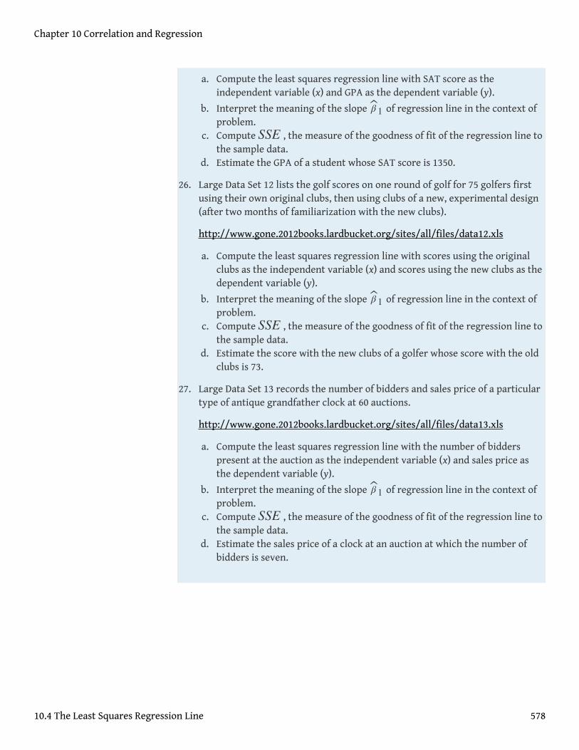
a. Compute the least squares regression line with SAT score as theindependent variable (x) and GPA as the dependent variable (y).
b. Interpret the meaning of the slope β 1 of regression line in the context ofproblem.
c. Compute SSE , the measure of the goodness of fit of the regression line tothe sample data.
d. Estimate the GPA of a student whose SAT score is 1350.
26. Large Data Set 12 lists the golf scores on one round of golf for 75 golfers firstusing their own original clubs, then using clubs of a new, experimental design(after two months of familiarization with the new clubs).
http://www.gone.2012books.lardbucket.org/sites/all/files/data12.xls
a. Compute the least squares regression line with scores using the originalclubs as the independent variable (x) and scores using the new clubs as thedependent variable (y).
b. Interpret the meaning of the slope β 1 of regression line in the context ofproblem.
c. Compute SSE , the measure of the goodness of fit of the regression line tothe sample data.
d. Estimate the score with the new clubs of a golfer whose score with the oldclubs is 73.
27. Large Data Set 13 records the number of bidders and sales price of a particulartype of antique grandfather clock at 60 auctions.
http://www.gone.2012books.lardbucket.org/sites/all/files/data13.xls
a. Compute the least squares regression line with the number of bidderspresent at the auction as the independent variable (x) and sales price asthe dependent variable (y).
b. Interpret the meaning of the slope β 1 of regression line in the context ofproblem.
c. Compute SSE , the measure of the goodness of fit of the regression line tothe sample data.
d. Estimate the sales price of a clock at an auction at which the number ofbidders is seven.
Chapter 10 Correlation and Regression
10.4 The Least Squares Regression Line 578
ANSWERS
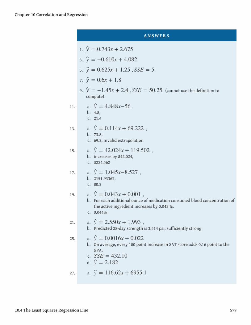
1. y = 0.743x + 2.675
3. y = −0.610x + 4.082
5. y = 0.625x + 1.25 , SSE = 5
7. y = 0.6x + 1.8
9. y = −1.45x + 2.4 , SSE = 50.25 (cannot use the definition tocompute)
11. a. y = 4.848x−56 ,b. 4.8,c. 21.6
13. a. y = 0.114x + 69.222 ,b. 73.8,c. 69.2, invalid extrapolation
15. a. y = 42.024x + 119.502 ,b. increases by $42,024,c. $224,562
17. a. y = 1.045x−8.527 ,b. 2151.93367,c. 80.3
19. a. y = 0.043x + 0.001 ,b. For each additional ounce of medication consumed blood concentration of
the active ingredient increases by 0.043 %,c. 0.044%
21. a. y = 2.550x + 1.993 ,b. Predicted 28-day strength is 3,514 psi; sufficiently strong
25. a. y = 0.0016x + 0.022b. On average, every 100 point increase in SAT score adds 0.16 point to the
GPA.c. SSE = 432.10d. y = 2.182
27. a. y = 116.62x + 6955.1
Chapter 10 Correlation and Regression
10.4 The Least Squares Regression Line 579
b. On average, every 1 additional bidder at an auction raises the price by116.62 dollars.
c. SSE = 1850314.08d. y = 7771.44
Chapter 10 Correlation and Regression
10.4 The Least Squares Regression Line 580
10.5 Statistical Inferences About β1
LEARNING OBJECTIVES
1. To learn how to construct a confidence interval for β1 , the slope of thepopulation regression line.
2. To learn how to test hypotheses regarding β1 .
The parameter β1 , the slope of the population regression line, is of primaryimportance in regression analysis because it gives the true rate of change in themean E (y) in response to a unit increase in the predictor variable x. For every unitincrease in x the mean of the response variable y changes by β1 units, increasing ifβ1 > 0 and decreasing if β1 < 0. We wish to construct confidence intervals for β1and test hypotheses about it.
Confidence Intervals for β1
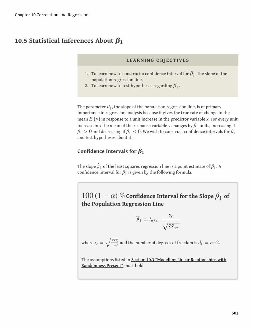
The slope β 1 of the least squares regression line is a point estimate of β1 . Aconfidence interval for β1 is given by the following formula.
100 (1 − α)% Confidence Interval for the Slope β1 ofthe Population Regression Line
where sε = SSEn−2
⎯ ⎯⎯⎯⎯⎯√ and the number of degrees of freedom is df = n−2.
The assumptions listed in Section 10.3 "Modelling Linear Relationships withRandomness Present" must hold.
β 1 ± tα∕2sε
SSxx⎯ ⎯⎯⎯⎯⎯⎯⎯
√
Chapter 10 Correlation and Regression
581
Definition
The statistic sε is called the sample standard deviation of errors7. It estimates thestandard deviation σ of the errors in the population of y-values for each fixed value of x(see Figure 10.5 "The Simple Linear Model Concept" in Section 10.3 "Modelling LinearRelationships with Randomness Present").
7. The statistic sε .
Chapter 10 Correlation and Regression
10.5 Statistical Inferences About β1 582
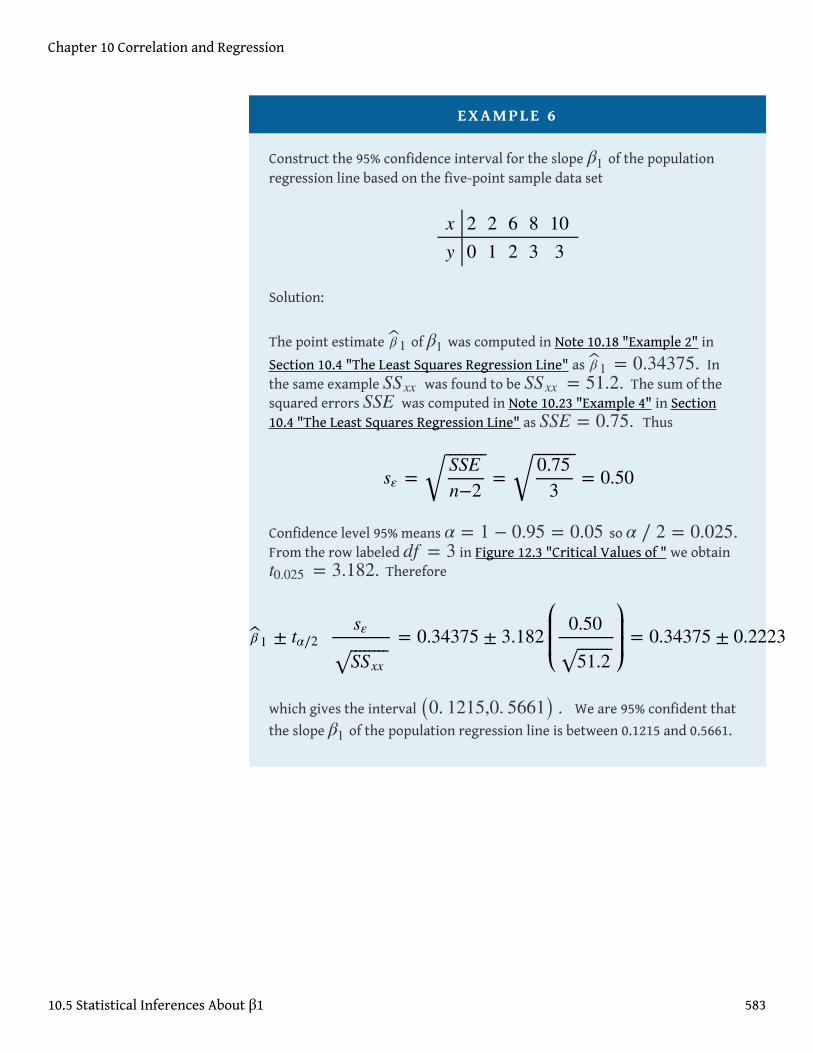
EXAMPLE 6
Construct the 95% confidence interval for the slope β1 of the populationregression line based on the five-point sample data set
Solution:
The point estimate β 1 of β1 was computed in Note 10.18 "Example 2" in
Section 10.4 "The Least Squares Regression Line" as β 1 = 0.34375. Inthe same example SSxx was found to be SSxx = 51.2. The sum of thesquared errors SSE was computed in Note 10.23 "Example 4" in Section10.4 "The Least Squares Regression Line" as SSE = 0.75. Thus
Confidence level 95% means α = 1 − 0.95 = 0.05 so α ∕ 2 = 0.025.From the row labeled df = 3 in Figure 12.3 "Critical Values of " we obtaint0.025 = 3.182. Therefore
which gives the interval (0. 1215,0. 5661) . We are 95% confident that
the slope β1 of the population regression line is between 0.1215 and 0.5661.
x
y
20
21
62
83
103
sε =SSE
n−2
⎯ ⎯⎯⎯⎯⎯⎯⎯
√ =0.753
⎯ ⎯⎯⎯⎯⎯⎯⎯⎯
√ = 0.50
β 1 ± tα∕2sε
SSxx⎯ ⎯⎯⎯⎯⎯⎯⎯
√= 0.34375 ± 3.182
0.50
51.2⎯ ⎯⎯⎯⎯⎯⎯
√
= 0.34375 ± 0.2223
Chapter 10 Correlation and Regression
10.5 Statistical Inferences About β1 583
EXAMPLE 7
Using the sample data in Table 10.3 "Data on Age and Value of UsedAutomobiles of a Specific Make and Model" construct a 90% confidenceinterval for the slope β1 of the population regression line relating age andvalue of the automobiles of Note 10.19 "Example 3" in Section 10.4 "TheLeast Squares Regression Line". Interpret the result in the context of theproblem.
Solution:
The point estimate β 1 of β1 was computed in Note 10.19 "Example 3", as
was SSxx . Their values are β 1 = −2.05 and SSxx = 14. The sum ofthe squared errors SSE was computed in Note 10.24 "Example 5" in Section10.4 "The Least Squares Regression Line" as SSE = 28.946. Thus
Confidence level 90% means α = 1 − 0.90 = 0.10 so α ∕ 2 = 0.05.From the row labeled df = 8 in Figure 12.3 "Critical Values of " we obtaint0.05 = 1.860. Therefore
which gives the interval (−3.00, −1.10) . We are 90% confident that theslope β1 of the population regression line is between −3.00 and −1.10. In thecontext of the problem this means that for vehicles of this make and modelbetween two and six years old we are 90% confident that for each additionalyear of age the average value of such a vehicle decreases by between $1,100and $3,000.
Testing Hypotheses About β1
Hypotheses regarding β1 can be tested using the same five-step procedures, eitherthe critical value approach or the p-value approach, that were introduced in Section8.1 "The Elements of Hypothesis Testing" and Section 8.3 "The Observed
sε =SSE
n−2
⎯ ⎯⎯⎯⎯⎯⎯⎯
√ =28.946
8
⎯ ⎯⎯⎯⎯⎯⎯⎯⎯⎯⎯⎯⎯
√ = 1.902169814
β 1 ± tα∕2sε
SSxx⎯ ⎯⎯⎯⎯⎯⎯⎯
√= −2.05 ± 1.860
1.902169814
14⎯ ⎯⎯⎯
√
= −2.05 ± 0.95
Chapter 10 Correlation and Regression
10.5 Statistical Inferences About β1 584
Significance of a Test" of Chapter 8 "Testing Hypotheses". The null hypothesisalways has the form H0 : β1 = B0 where B0 is a number determined from the
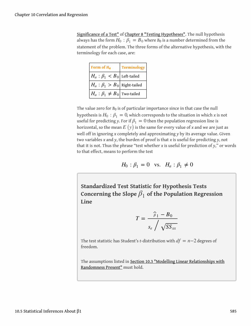
statement of the problem. The three forms of the alternative hypothesis, with theterminology for each case, are:
Form of Ha Terminology
Ha : β1 < B0 Left-tailed
Ha : β1 > B0 Right-tailed
Ha : β1 ≠ B0 Two-tailed
The value zero for B0 is of particular importance since in that case the null
hypothesis is H0 : β1 = 0, which corresponds to the situation in which x is notuseful for predicting y. For if β1 = 0 then the population regression line ishorizontal, so the mean E (y) is the same for every value of x and we are just aswell off in ignoring x completely and approximating y by its average value. Giventwo variables x and y, the burden of proof is that x is useful for predicting y, notthat it is not. Thus the phrase “test whether x is useful for prediction of y,” or wordsto that effect, means to perform the test
Standardized Test Statistic for Hypothesis TestsConcerning the Slope β1 of the Population RegressionLine
The test statistic has Student’s t-distribution with df = n−2 degrees offreedom.
The assumptions listed in Section 10.3 "Modelling Linear Relationships withRandomness Present" must hold.
H0 : β1 = 0 vs. Ha : β1 ≠ 0
T =β 1 − B0
sε / SSxx⎯ ⎯⎯⎯⎯⎯⎯⎯
√
Chapter 10 Correlation and Regression
10.5 Statistical Inferences About β1 585
EXAMPLE 8
Test, at the 2% level of significance, whether the variable x is useful forpredicting y based on the information in the five-point data set
Solution:
We will perform the test using the critical value approach.
• Step 1. Since x is useful for prediction of y precisely when theslope β1 of the population regression line is nonzero, therelevant test is
• Step 2. The test statistic is
and has Student’s t-distribution with n−2 = 5 − 2 = 3degrees of freedom.
• Step 3. From Note 10.18 "Example 2", β 1 = 0.34375 andSSxx = 51.2. From Note 10.30 "Example 6", sε = 0.50. Thevalue of the test statistic is therefore
• Step 4. Since the symbol in Ha is “≠” this is a two-tailed test, so there aretwo critical values ±tα∕2 = ±t0.01 . Reading from the line in Figure
x
y
20
21
62
83
103
H0 : β1 = 0vs. Ha : β1 ≠ 0 @α = 0.02
T =β 1
sε / SSxx⎯ ⎯⎯⎯⎯⎯⎯⎯
√
T =β 1 − B0
sε / SSxx⎯ ⎯⎯⎯⎯⎯⎯⎯
√=
0.34375
0.50 / 51.2⎯ ⎯⎯⎯⎯⎯⎯
√= 4.919
Chapter 10 Correlation and Regression
10.5 Statistical Inferences About β1 586
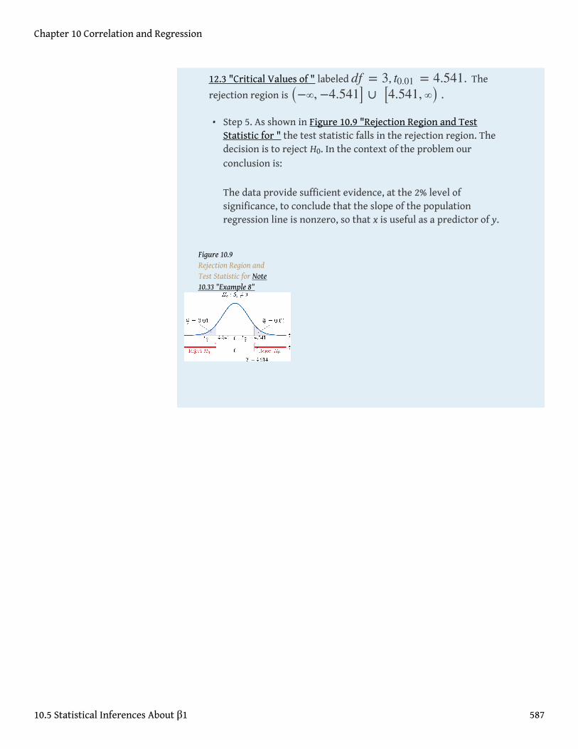
12.3 "Critical Values of " labeled df = 3, t0.01 = 4.541. The
rejection region is (−∞, −4.541] ∪ [4.541, ∞) .• Step 5. As shown in Figure 10.9 "Rejection Region and Test
Statistic for " the test statistic falls in the rejection region. Thedecision is to reject H0. In the context of the problem ourconclusion is:
The data provide sufficient evidence, at the 2% level ofsignificance, to conclude that the slope of the populationregression line is nonzero, so that x is useful as a predictor of y.
Figure 10.9Rejection Region andTest Statistic for Note10.33 "Example 8"
Chapter 10 Correlation and Regression
10.5 Statistical Inferences About β1 587

EXAMPLE 9
A car salesman claims that automobiles between two and six years old of themake and model discussed in Note 10.19 "Example 3" in Section 10.4 "TheLeast Squares Regression Line" lose more than $1,100 in value each year.Test this claim at the 5% level of significance.
Solution:
We will perform the test using the critical value approach.
• Step 1. In terms of the variables x and y, the salesman’s claim isthat if x is increased by 1 unit (one additional year in age), then ydecreases by more than 1.1 units (more than $1,100). Thus hisassertion is that the slope of the population regression line isnegative, and that it is more negative than −1.1. In symbols,β1 < −1.1. Since it contains an inequality, this has to be thealternative hypotheses. The null hypothesis has to be an equalityand have the same number on the right hand side, so therelevant test is
• Step 2. The test statistic is
and has Student’s t-distribution with 8 degrees of freedom.
• Step 3. From Note 10.19 "Example 3", β 1 = −2.05 andSSxx = 14. From Note 10.31 "Example 7",sε = 1.902169814. The value of the test statistic istherefore
H0 : β1 = −1.1vs. Hα : β1 < −1.1 @α = 0.05
T =β 1 − B0
sε / SSxx⎯ ⎯⎯⎯⎯⎯⎯⎯
√
Chapter 10 Correlation and Regression
10.5 Statistical Inferences About β1 588
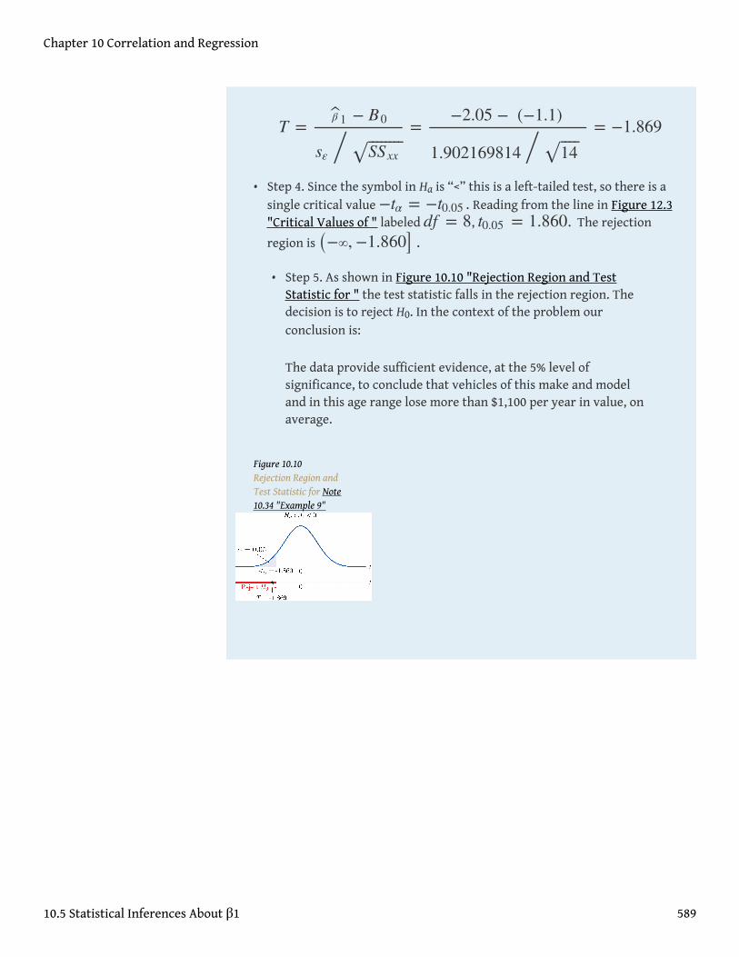
• Step 4. Since the symbol in Ha is “<” this is a left-tailed test, so there is asingle critical value −tα = −t0.05 . Reading from the line in Figure 12.3"Critical Values of " labeled df = 8, t0.05 = 1.860. The rejection
region is (−∞, −1.860] .• Step 5. As shown in Figure 10.10 "Rejection Region and Test
Statistic for " the test statistic falls in the rejection region. Thedecision is to reject H0. In the context of the problem ourconclusion is:
The data provide sufficient evidence, at the 5% level ofsignificance, to conclude that vehicles of this make and modeland in this age range lose more than $1,100 per year in value, onaverage.
Figure 10.10Rejection Region andTest Statistic for Note10.34 "Example 9"
T =β 1 − B0
sε / SSxx⎯ ⎯⎯⎯⎯⎯⎯⎯
√=
−2.05 − (−1.1)
1.902169814 / 14⎯ ⎯⎯⎯
√= −1.869
Chapter 10 Correlation and Regression
10.5 Statistical Inferences About β1 589
KEY TAKEAWAYS
• The parameter β1 , the slope of the population regression line, is ofprimary interest because it describes the average change in y withrespect to unit increase in x.
• The statistic β 1 , the slope of the least squares regression line, is a pointestimate of β1 . Confidence intervals for β1 can be computed using aformula.
• Hypotheses regarding β1 are tested using the same five-step proceduresintroduced in Chapter 8 "Testing Hypotheses".
Chapter 10 Correlation and Regression
10.5 Statistical Inferences About β1 590
EXERCISES
BASIC
For the Basic and Application exercises in this section use the computationsthat were done for the exercises with the same number in Section 10.2 "TheLinear Correlation Coefficient" and Section 10.4 "The Least SquaresRegression Line".
1. Construct the 95% confidence interval for the slope β1 of the populationregression line based on the sample data set of Exercise 1 of Section 10.2 "TheLinear Correlation Coefficient".
2. Construct the 90% confidence interval for the slope β1 of the populationregression line based on the sample data set of Exercise 2 of Section 10.2 "TheLinear Correlation Coefficient".
3. Construct the 90% confidence interval for the slope β1 of the populationregression line based on the sample data set of Exercise 3 of Section 10.2 "TheLinear Correlation Coefficient".
4. Construct the 99% confidence interval for the slope β1 of the populationregression Exercise 4 of Section 10.2 "The Linear Correlation Coefficient".
5. For the data in Exercise 5 of Section 10.2 "The Linear Correlation Coefficient"test, at the 10% level of significance, whether x is useful for predicting y (thatis, whether β1 ≠ 0).
6. For the data in Exercise 6 of Section 10.2 "The Linear Correlation Coefficient"test, at the 5% level of significance, whether x is useful for predicting y (that is,whether β1 ≠ 0).
7. Construct the 90% confidence interval for the slope β1 of the populationregression line based on the sample data set of Exercise 7 of Section 10.2 "TheLinear Correlation Coefficient".
8. Construct the 95% confidence interval for the slope β1 of the populationregression line based on the sample data set of Exercise 8 of Section 10.2 "TheLinear Correlation Coefficient".
9. For the data in Exercise 9 of Section 10.2 "The Linear Correlation Coefficient"test, at the 1% level of significance, whether x is useful for predicting y (that is,whether β1 ≠ 0).
Chapter 10 Correlation and Regression
10.5 Statistical Inferences About β1 591
10. For the data in Exercise 10 of Section 10.2 "The Linear Correlation Coefficient"test, at the 1% level of significance, whether x is useful for predicting y (that is,whether β1 ≠ 0).
APPLICATIONS
11. For the data in Exercise 11 of Section 10.2 "The Linear Correlation Coefficient"construct a 90% confidence interval for the mean number of new wordsacquired per month by children between 13 and 18 months of age.
12. For the data in Exercise 12 of Section 10.2 "The Linear Correlation Coefficient"construct a 90% confidence interval for the mean increased braking distancefor each additional 100 pounds of vehicle weight.
13. For the data in Exercise 13 of Section 10.2 "The Linear Correlation Coefficient"test, at the 10% level of significance, whether age is useful for predictingresting heart rate.
14. For the data in Exercise 14 of Section 10.2 "The Linear Correlation Coefficient"test, at the 10% level of significance, whether wind speed is useful forpredicting wave height.
15. For the situation described in Exercise 15 of Section 10.2 "The LinearCorrelation Coefficient"
a. Construct the 95% confidence interval for the mean increase in revenueper additional thousand dollars spent on advertising.
b. An advertising agency tells the business owner that for every additionalthousand dollars spent on advertising, revenue will increase by over$25,000. Test this claim (which is the alternative hypothesis) at the 5%level of significance.
c. Perform the test of part (b) at the 10% level of significance.d. Based on the results in (b) and (c), how believable is the ad agency’s claim?
(This is a subjective judgement.)
16. For the situation described in Exercise 16 of Section 10.2 "The LinearCorrelation Coefficient"
a. Construct the 90% confidence interval for the mean increase in height peradditional inch of length at age two.
b. It is claimed that for girls each additional inch of length at age two meansmore than an additional inch of height at maturity. Test this claim (whichis the alternative hypothesis) at the 10% level of significance.
Chapter 10 Correlation and Regression
10.5 Statistical Inferences About β1 592
17. For the data in Exercise 17 of Section 10.2 "The Linear Correlation Coefficient"test, at the 10% level of significance, whether course average before the finalexam is useful for predicting the final exam grade.
18. For the situation described in Exercise 18 of Section 10.2 "The LinearCorrelation Coefficient", an agronomist claims that each additional millionacres planted results in more than 750,000 additional acres harvested. Test thisclaim at the 1% level of significance.
19. For the data in Exercise 19 of Section 10.2 "The Linear Correlation Coefficient"test, at the 1/10th of 1% level of significance, whether, ignoring all other factssuch as age and body mass, the amount of the medication consumed is a usefulpredictor of blood concentration of the active ingredient.
20. For the data in Exercise 20 of Section 10.2 "The Linear Correlation Coefficient"test, at the 1% level of significance, whether for each additional inch of girththe age of the tree increases by at least two and one-half years.
21. For the data in Exercise 21 of Section 10.2 "The Linear Correlation Coefficient"
a. Construct the 95% confidence interval for the mean increase in strength at28 days for each additional hundred psi increase in strength at 3 days.
b. Test, at the 1/10th of 1% level of significance, whether the 3-day strengthis useful for predicting 28-day strength.
22. For the situation described in Exercise 22 of Section 10.2 "The LinearCorrelation Coefficient"
a. Construct the 99% confidence interval for the mean decrease in energydemand for each one-degree drop in temperature.
b. An engineer with the power company believes that for each one-degreeincrease in temperature, daily energy demand will decrease by more than3.6 million watt-hours. Test this claim at the 1% level of significance.
LARGE DATA SET EXERCISES
23. Large Data Set 1 lists the SAT scores and GPAs of 1,000 students.
http://www.gone.2012books.lardbucket.org/sites/all/files/data1.xls
a. Compute the 90% confidence interval for the slope β1 of the populationregression line with SAT score as the independent variable (x) and GPA asthe dependent variable (y).
Chapter 10 Correlation and Regression
10.5 Statistical Inferences About β1 593
b. Test, at the 10% level of significance, the hypothesis that the slope of thepopulation regression line is greater than 0.001, against the nullhypothesis that it is exactly 0.001.
24. Large Data Set 12 lists the golf scores on one round of golf for 75 golfers firstusing their own original clubs, then using clubs of a new, experimental design(after two months of familiarization with the new clubs).
http://www.gone.2012books.lardbucket.org/sites/all/files/data12.xls
a. Compute the 95% confidence interval for the slope β1 of the populationregression line with scores using the original clubs as the independentvariable (x) and scores using the new clubs as the dependent variable (y).
b. Test, at the 10% level of significance, the hypothesis that the slope of thepopulation regression line is different from 1, against the null hypothesisthat it is exactly 1.
25. Large Data Set 13 records the number of bidders and sales price of a particulartype of antique grandfather clock at 60 auctions.
http://www.gone.2012books.lardbucket.org/sites/all/files/data13.xls
a. Compute the 95% confidence interval for the slope β1 of the populationregression line with the number of bidders present at the auction as theindependent variable (x) and sales price as the dependent variable (y).
b. Test, at the 10% level of significance, the hypothesis that the average salesprice increases by more than $90 for each additional bidder at an auction,against the default that it increases by exactly $90.
Chapter 10 Correlation and Regression
10.5 Statistical Inferences About β1 594
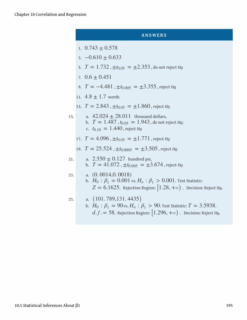
ANSWERS
1. 0.743 ± 0.5783. −0.610 ± 0.6335. T = 1.732 , ±t0.05 = ±2.353 , do not reject H0
7. 0.6 ± 0.4519. T = −4.481 , ±t0.005 = ±3.355 , reject H0
11. 4.8 ± 1.7 words
13. T = 2.843 , ±t0.05 = ±1.860 , reject H0
15. a. 42.024 ± 28.011 thousand dollars,b. T = 1.487 , t0.05 = 1.943 , do not reject H0;c. t0.10 = 1.440 , reject H0
17. T = 4.096 , ±t0.05 = ±1.771 , reject H0
19. T = 25.524 , ±t0.0005 = ±3.505 , reject H0
21. a. 2.550 ± 0.127 hundred psi,b. T = 41.072 , ±t0.005 = ±3.674 , reject H0
23. a. (0. 0014,0. 0018)b. H0 : β1 = 0.001 vs. Ha : β1 > 0.001. Test Statistic:
Z = 6.1625. Rejection Region: [1.28, +∞) . Decision: Reject H0.
25. a. (101. 789,131. 4435)b. H0 : β1 = 90vs. Ha : β1 > 90.Test Statistic: T = 3.5938.
d. f . = 58. Rejection Region: [1.296, +∞) . Decision: Reject H0.
Chapter 10 Correlation and Regression
10.5 Statistical Inferences About β1 595
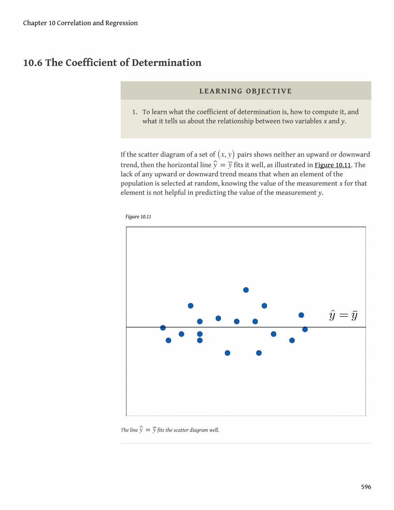
10.6 The Coefficient of Determination
LEARNING OBJECTIVE
1. To learn what the coefficient of determination is, how to compute it, andwhat it tells us about the relationship between two variables x and y.
If the scatter diagram of a set of (x, y) pairs shows neither an upward or downward
trend, then the horizontal line y = y⎯⎯ fits it well, as illustrated in Figure 10.11. Thelack of any upward or downward trend means that when an element of thepopulation is selected at random, knowing the value of the measurement x for thatelement is not helpful in predicting the value of the measurement y.
Figure 10.11
The line y = y⎯⎯ fits the scatter diagram well.
Chapter 10 Correlation and Regression
596
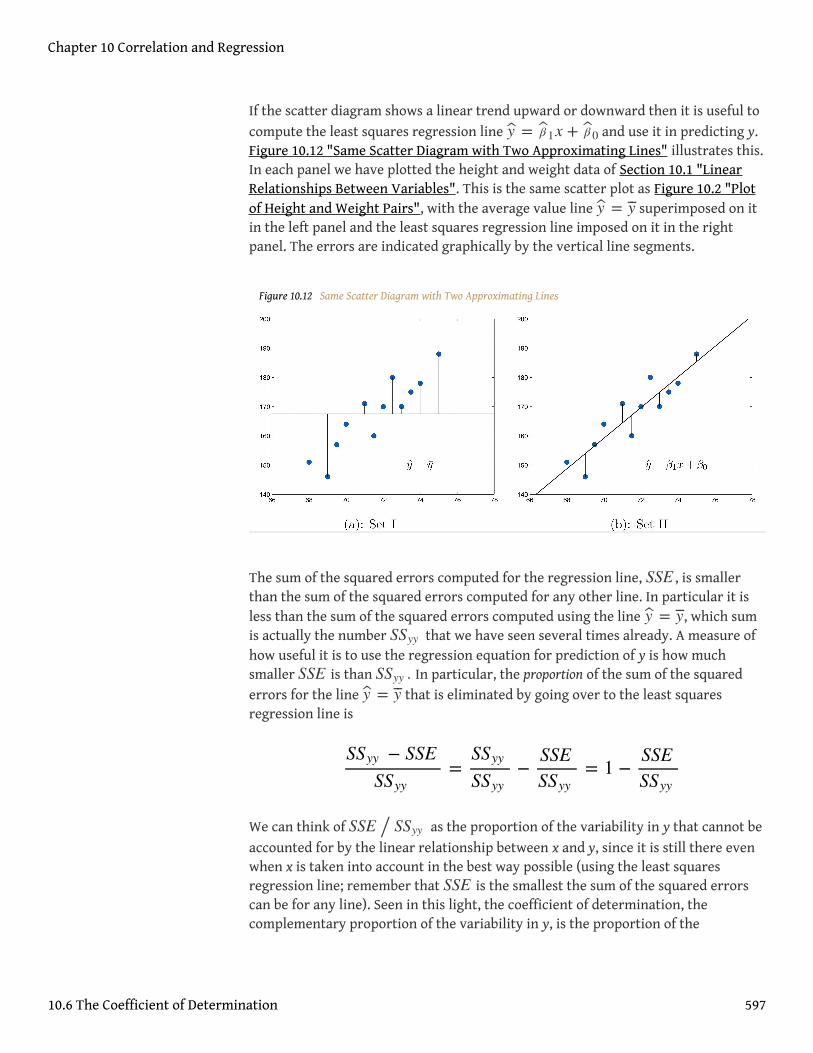
If the scatter diagram shows a linear trend upward or downward then it is useful tocompute the least squares regression line y = β 1x + β 0 and use it in predicting y.Figure 10.12 "Same Scatter Diagram with Two Approximating Lines" illustrates this.In each panel we have plotted the height and weight data of Section 10.1 "LinearRelationships Between Variables". This is the same scatter plot as Figure 10.2 "Plotof Height and Weight Pairs", with the average value line y = y⎯⎯ superimposed on itin the left panel and the least squares regression line imposed on it in the rightpanel. The errors are indicated graphically by the vertical line segments.
Figure 10.12 Same Scatter Diagram with Two Approximating Lines
The sum of the squared errors computed for the regression line, SSE , is smallerthan the sum of the squared errors computed for any other line. In particular it isless than the sum of the squared errors computed using the line y = y⎯⎯, which sumis actually the number SSyy that we have seen several times already. A measure ofhow useful it is to use the regression equation for prediction of y is how muchsmaller SSE is than SSyy . In particular, the proportion of the sum of the squarederrors for the line y = y⎯⎯ that is eliminated by going over to the least squaresregression line is
We can think of SSE / SSyy as the proportion of the variability in y that cannot beaccounted for by the linear relationship between x and y, since it is still there evenwhen x is taken into account in the best way possible (using the least squaresregression line; remember that SSE is the smallest the sum of the squared errorscan be for any line). Seen in this light, the coefficient of determination, thecomplementary proportion of the variability in y, is the proportion of the
SSyy − SSE
SSyy=
SSyy
SSyy−
SSE
SSyy= 1 −
SSE
SSyy
Chapter 10 Correlation and Regression
10.6 The Coefficient of Determination 597
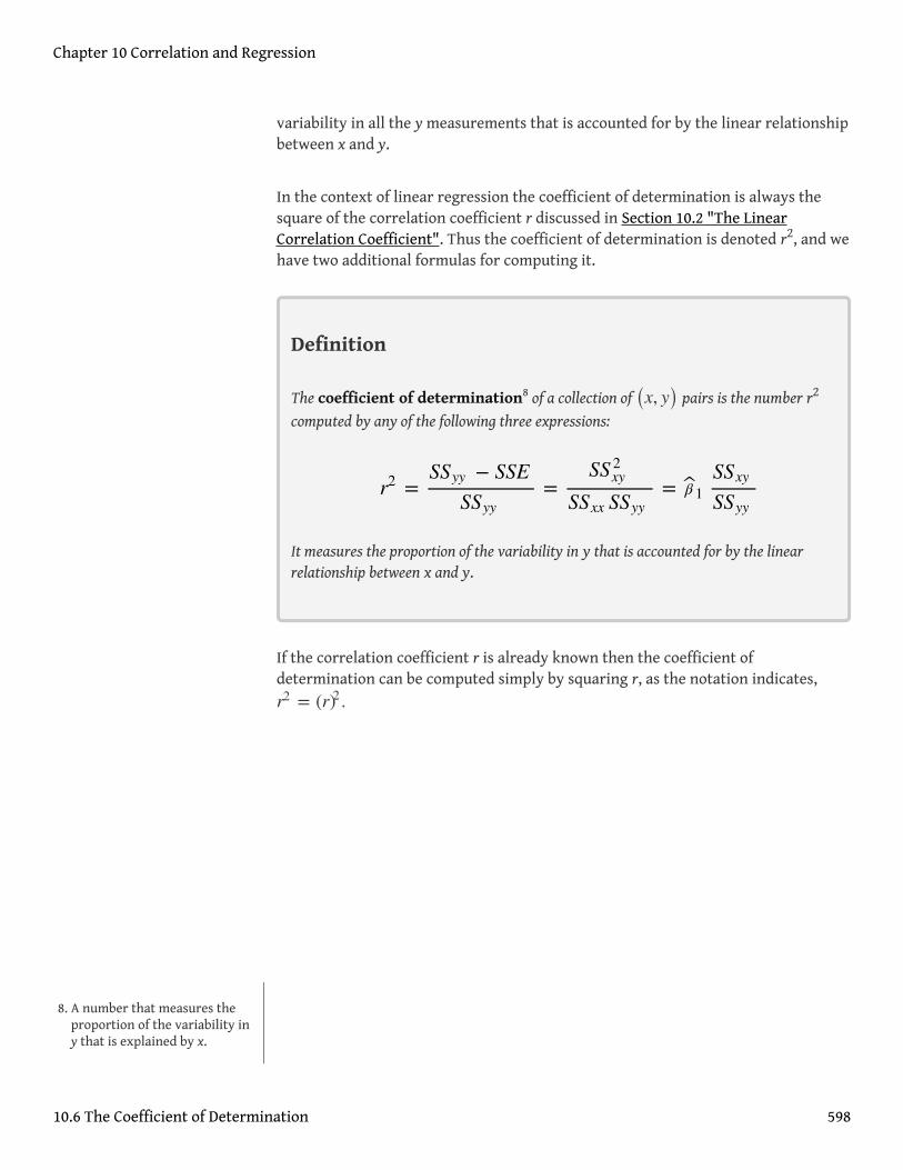
variability in all the y measurements that is accounted for by the linear relationshipbetween x and y.
In the context of linear regression the coefficient of determination is always thesquare of the correlation coefficient r discussed in Section 10.2 "The LinearCorrelation Coefficient". Thus the coefficient of determination is denoted r2, and wehave two additional formulas for computing it.
Definition
The coefficient of determination8 of a collection of (x, y) pairs is the number r2
computed by any of the following three expressions:
It measures the proportion of the variability in y that is accounted for by the linearrelationship between x and y.
If the correlation coefficient r is already known then the coefficient ofdetermination can be computed simply by squaring r, as the notation indicates,r2 = (r)2 .
r2 =SSyy − SSE
SSyy=
SS 2xy
SSxx SSyy= β 1
SSxy
SSyy
8. A number that measures theproportion of the variability iny that is explained by x.
Chapter 10 Correlation and Regression
10.6 The Coefficient of Determination 598

EXAMPLE 10
The value of used vehicles of the make and model discussed in Note 10.19"Example 3" in Section 10.4 "The Least Squares Regression Line" varieswidely. The most expensive automobile in the sample in Table 10.3 "Data onAge and Value of Used Automobiles of a Specific Make and Model" has value$30,500, which is nearly half again as much as the least expensive one, whichis worth $20,400. Find the proportion of the variability in value that isaccounted for by the linear relationship between age and value.
Solution:
The proportion of the variability in value y that is accounted for by thelinear relationship between it and age x is given by the coefficient ofdetermination, r2. Since the correlation coefficient r was already computed
in Note 10.19 "Example 3" as r = −0.819 , r2 = (−0.819) 2 = 0.671.About 67% of the variability in the value of this vehicle can be explained byits age.
Chapter 10 Correlation and Regression
10.6 The Coefficient of Determination 599
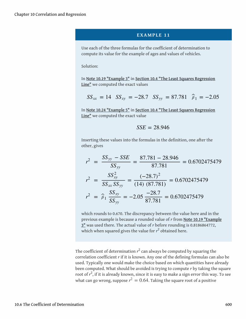
EXAMPLE 11
Use each of the three formulas for the coefficient of determination tocompute its value for the example of ages and values of vehicles.
Solution:
In Note 10.19 "Example 3" in Section 10.4 "The Least Squares RegressionLine" we computed the exact values
In Note 10.24 "Example 5" in Section 10.4 "The Least Squares RegressionLine" we computed the exact value
Inserting these values into the formulas in the definition, one after theother, gives
which rounds to 0.670. The discrepancy between the value here and in theprevious example is because a rounded value of r from Note 10.19 "Example3" was used there. The actual value of r before rounding is 0.8186864772,which when squared gives the value for r2 obtained here.
The coefficient of determination r2 can always be computed by squaring thecorrelation coefficient r if it is known. Any one of the defining formulas can also beused. Typically one would make the choice based on which quantities have alreadybeen computed. What should be avoided is trying to compute r by taking the squareroot of r2, if it is already known, since it is easy to make a sign error this way. To seewhat can go wrong, suppose r2 = 0.64. Taking the square root of a positive
SSxx = 14 SSxy = −28.7 SSyy = 87.781 β 1 = −2.05
SSE = 28.946
r2
r2
r2
=
=
=
SSyy − SSE
SSyy=
87.781 − 28.94687.781
= 0.6702475479
SS 2xy
SSxx SSyy=
(−28.7)2
(14) (87.781)= 0.6702475479
β 1SSxy
SSyy= −2.05
−28.787.781
= 0.6702475479
Chapter 10 Correlation and Regression
10.6 The Coefficient of Determination 600
number with any calculating device will always return a positive result. The squareroot of 0.64 is 0.8. However, the actual value of r might be the negative number −0.8.
KEY TAKEAWAYS
• The coefficient of determination r2 estimates the proportion of thevariability in the variable y that is explained by the linear relationshipbetween y and the variable x.
• There are several formulas for computing r2. The choice of which one touse can be based on which quantities have already been computed sofar.
Chapter 10 Correlation and Regression
10.6 The Coefficient of Determination 601
EXERCISES
BASIC
For the Basic and Application exercises in this section use the computationsthat were done for the exercises with the same number in Section 10.2 "TheLinear Correlation Coefficient", Section 10.4 "The Least Squares RegressionLine", and Section 10.5 "Statistical Inferences About ".
1. For the sample data set of Exercise 1 of Section 10.2 "The Linear CorrelationCoefficient" find the coefficient of determination using the formula
r2 = β 1SSxy / SSyy . Confirm your answer by squaring r as computed inthat exercise.
2. For the sample data set of Exercise 2 of Section 10.2 "The Linear CorrelationCoefficient" find the coefficient of determination using the formula
r2 = β 1SSxy / SSyy . Confirm your answer by squaring r as computed inthat exercise.
3. For the sample data set of Exercise 3 of Section 10.2 "The Linear CorrelationCoefficient" find the coefficient of determination using the formula
r2 = β 1SSxy / SSyy . Confirm your answer by squaring r as computed inthat exercise.
4. For the sample data set of Exercise 4 of Section 10.2 "The Linear CorrelationCoefficient" find the coefficient of determination using the formula
r2 = β 1SSxy / SSyy . Confirm your answer by squaring r as computed inthat exercise.
5. For the sample data set of Exercise 5 of Section 10.2 "The Linear CorrelationCoefficient" find the coefficient of determination using the formula
r2 = β 1SSxy / SSyy . Confirm your answer by squaring r as computed inthat exercise.
6. For the sample data set of Exercise 6 of Section 10.2 "The Linear CorrelationCoefficient" find the coefficient of determination using the formula
r2 = β 1SSxy / SSyy . Confirm your answer by squaring r as computed inthat exercise.
7. For the sample data set of Exercise 7 of Section 10.2 "The Linear CorrelationCoefficient" find the coefficient of determination using the formula
Chapter 10 Correlation and Regression
10.6 The Coefficient of Determination 602
r2 = (SSyy − SSE) / SSyy . Confirm your answer by squaring r as
computed in that exercise.
8. For the sample data set of Exercise 8 of Section 10.2 "The Linear CorrelationCoefficient" find the coefficient of determination using the formula
r2 = (SSyy − SSE) / SSyy . Confirm your answer by squaring r as
computed in that exercise.
9. For the sample data set of Exercise 9 of Section 10.2 "The Linear CorrelationCoefficient" find the coefficient of determination using the formula
r2 = (SSyy − SSE) / SSyy . Confirm your answer by squaring r as
computed in that exercise.
10. For the sample data set of Exercise 9 of Section 10.2 "The Linear CorrelationCoefficient" find the coefficient of determination using the formula
r2 = (SSyy − SSE) / SSyy . Confirm your answer by squaring r as
computed in that exercise.
APPLICATIONS
11. For the data in Exercise 11 of Section 10.2 "The Linear Correlation Coefficient"compute the coefficient of determination and interpret its value in the contextof age and vocabulary.
12. For the data in Exercise 12 of Section 10.2 "The Linear Correlation Coefficient"compute the coefficient of determination and interpret its value in the contextof vehicle weight and braking distance.
13. For the data in Exercise 13 of Section 10.2 "The Linear Correlation Coefficient"compute the coefficient of determination and interpret its value in the contextof age and resting heart rate. In the age range of the data, does age seem to bea very important factor with regard to heart rate?
14. For the data in Exercise 14 of Section 10.2 "The Linear Correlation Coefficient"compute the coefficient of determination and interpret its value in the contextof wind speed and wave height. Does wind speed seem to be a very importantfactor with regard to wave height?
15. For the data in Exercise 15 of Section 10.2 "The Linear Correlation Coefficient"find the proportion of the variability in revenue that is explained by level ofadvertising.
Chapter 10 Correlation and Regression
10.6 The Coefficient of Determination 603
16. For the data in Exercise 16 of Section 10.2 "The Linear Correlation Coefficient"find the proportion of the variability in adult height that is explained by thevariation in length at age two.
17. For the data in Exercise 17 of Section 10.2 "The Linear Correlation Coefficient"compute the coefficient of determination and interpret its value in the contextof course average before the final exam and score on the final exam.
18. For the data in Exercise 18 of Section 10.2 "The Linear Correlation Coefficient"compute the coefficient of determination and interpret its value in the contextof acres planted and acres harvested.
19. For the data in Exercise 19 of Section 10.2 "The Linear Correlation Coefficient"compute the coefficient of determination and interpret its value in the contextof the amount of the medication consumed and blood concentration of theactive ingredient.
20. For the data in Exercise 20 of Section 10.2 "The Linear Correlation Coefficient"compute the coefficient of determination and interpret its value in the contextof tree size and age.
21. For the data in Exercise 21 of Section 10.2 "The Linear Correlation Coefficient"find the proportion of the variability in 28-day strength of concrete that isaccounted for by variation in 3-day strength.
22. For the data in Exercise 22 of Section 10.2 "The Linear Correlation Coefficient"find the proportion of the variability in energy demand that is accounted forby variation in average temperature.
LARGE DATA SET EXERCISES
23. Large Data Set 1 lists the SAT scores and GPAs of 1,000 students. Compute thecoefficient of determination and interpret its value in the context of SATscores and GPAs.
http://www.gone.2012books.lardbucket.org/sites/all/files/data1.xls
24. Large Data Set 12 lists the golf scores on one round of golf for 75 golfers firstusing their own original clubs, then using clubs of a new, experimental design(after two months of familiarization with the new clubs). Compute thecoefficient of determination and interpret its value in the context of golfscores with the two kinds of golf clubs.
http://www.gone.2012books.lardbucket.org/sites/all/files/data12.xls
Chapter 10 Correlation and Regression
10.6 The Coefficient of Determination 604
25. Large Data Set 13 records the number of bidders and sales price of a particulartype of antique grandfather clock at 60 auctions. Compute the coefficient ofdetermination and interpret its value in the context of the number of biddersat an auction and the price of this type of antique grandfather clock.
http://www.gone.2012books.lardbucket.org/sites/all/files/data13.xls
ANSWERS
1. 0.848
3. 0.631
5. 0.5
7. 0.766
9. 0.715
11. 0.898; about 90% of the variability in vocabulary is explained by age
13. 0.503; about 50% of the variability in heart rate is explained by age. Age is asignificant but not dominant factor in explaining heart rate.
15. The proportion is r2 = 0.692.
17. 0.563; about 56% of the variability in final exam scores is explained by courseaverage before the final exam
19. 0.931; about 93% of the variability in the blood concentration of the activeingredient is explained by the amount of the medication consumed
21. The proportion is r2 = 0.984.
23. r2 = 21.17%.
25. r2 = 81.04%.
Chapter 10 Correlation and Regression
10.6 The Coefficient of Determination 605

10.7 Estimation and Prediction
LEARNING OBJECTIVES
1. To learn the distinction between estimation and prediction.2. To learn the distinction between a confidence interval and a prediction
interval.3. To learn how to implement formulas for computing confidence intervals
and prediction intervals.
Consider the following pairs of problems, in the context of Note 10.19 "Example 3"in Section 10.4 "The Least Squares Regression Line", the automobile age and valueexample.
1.
1. Estimate the average value of all four-year-old automobiles of thismake and model.
2. Construct a 95% confidence interval for the average value of allfour-year-old automobiles of this make and model.
2.
1. Shylock intends to buy a four-year-old automobile of this makeand model next week. Predict the value of the first suchautomobile that he encounters.
2. Construct a 95% confidence interval for the value of the first suchautomobile that he encounters.
The method of solution and answer to the first question in each pair, (1a) and (2a),are the same. When we set x equal to 4 in the least squares regression equationy = −2.05x + 32.83 that was computed in part (c) of Note 10.19 "Example 3" inSection 10.4 "The Least Squares Regression Line", the number returned,
which corresponds to value $24,630, is an estimate of precisely the number soughtin question (1a): the mean E (y) of all y values when x = 4. Since nothing is knownabout the first four-year-old automobile of this make and model that Shylock will
y = −2.05 (4) + 32.83 = 24.63
Chapter 10 Correlation and Regression
606

encounter, our best guess as to its value is the mean value E (y) of all suchautomobiles, the number 24.63 or $24,630, computed in the same way.
The answers to the second part of each question differ. In question (1b) we aretrying to estimate a population parameter: the mean of the all the y-values in thesub-population picked out by the value x = 4, that is, the average value of all four-year-old automobiles. In question (2b), however, we are not trying to capture afixed parameter, but the value of the random variable y in one trial of anexperiment: examine the first four-year-old car Shylock encounters. In the firstcase we seek to construct a confidence interval in the same sense that we have donebefore. In the second case the situation is different, and the interval constructedhas a different name, prediction interval. In the second case we are trying to“predict” where a the value of a random variable will take its value.
100 (1 − α)% Confidence Interval for the Mean Valueof y at x = xp
where
a. xp is a particular value of x that lies in the range of x-values in the
sample data set used to construct the least squares regression line;b. yp is the numerical value obtained when the least square
regression equation is evaluated at x = xp ; andc. the number of degrees of freedom for tα∕2 is df = n−2.
The assumptions listed in Section 10.3 "Modelling Linear Relationships withRandomness Present" must hold.
The formula for the prediction interval is identical except for the presence of thenumber 1 underneath the square root sign. This means that the prediction intervalis always wider than the confidence interval at the same confidence level and valueof x. In practice the presence of the number 1 tends to make it much wider.
yp ± tα∕2 sε1n
+ (xp − x⎯⎯)2SSxx
⎯ ⎯⎯⎯⎯⎯⎯⎯⎯⎯⎯⎯⎯⎯⎯⎯⎯⎯⎯⎯⎯⎯⎯⎯
√
Chapter 10 Correlation and Regression
10.7 Estimation and Prediction 607
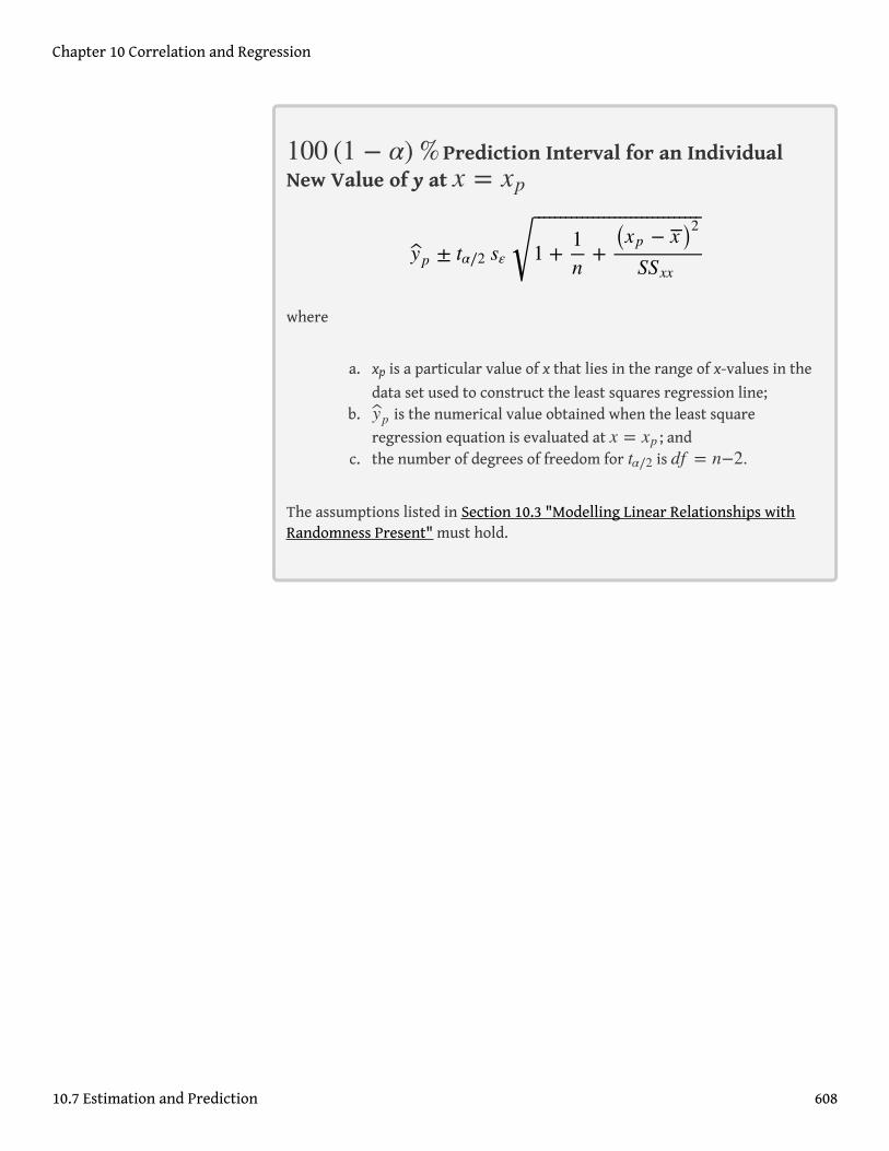
100 (1 − α)%Prediction Interval for an IndividualNew Value of y at x = xp
where
a. xp is a particular value of x that lies in the range of x-values in the
data set used to construct the least squares regression line;b. yp is the numerical value obtained when the least square
regression equation is evaluated at x = xp ; andc. the number of degrees of freedom for tα∕2 is df = n−2.
The assumptions listed in Section 10.3 "Modelling Linear Relationships withRandomness Present" must hold.
yp ± tα∕2 sε 1 +1n
+ (xp − x⎯⎯)2SSxx
⎯ ⎯⎯⎯⎯⎯⎯⎯⎯⎯⎯⎯⎯⎯⎯⎯⎯⎯⎯⎯⎯⎯⎯⎯⎯⎯⎯⎯⎯⎯⎯
√
Chapter 10 Correlation and Regression
10.7 Estimation and Prediction 608
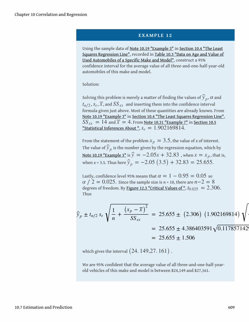
EXAMPLE 12
Using the sample data of Note 10.19 "Example 3" in Section 10.4 "The LeastSquares Regression Line", recorded in Table 10.3 "Data on Age and Value ofUsed Automobiles of a Specific Make and Model", construct a 95%confidence interval for the average value of all three-and-one-half-year-oldautomobiles of this make and model.
Solution:
Solving this problem is merely a matter of finding the values of yp , α and
tα∕2 , sε , x⎯⎯, and SSxx and inserting them into the confidence intervalformula given just above. Most of these quantities are already known. FromNote 10.19 "Example 3" in Section 10.4 "The Least Squares Regression Line",SSxx = 14 and x⎯⎯ = 4. From Note 10.31 "Example 7" in Section 10.5"Statistical Inferences About ", sε = 1.902169814.
From the statement of the problem xp = 3.5, the value of x of interest.
The value of yp is the number given by the regression equation, which by
Note 10.19 "Example 3" is y = −2.05x + 32.83 , when x = xp , that is,
when x = 3.5. Thus here yp = −2.05 (3.5) + 32.83 = 25.655.
Lastly, confidence level 95% means that α = 1 − 0.95 = 0.05 soα ∕ 2 = 0.025. Since the sample size is n = 10, there are n−2 = 8degrees of freedom. By Figure 12.3 "Critical Values of ", t0.025 = 2.306.Thus
which gives the interval (24. 149,27. 161) .We are 95% confident that the average value of all three-and-one-half-year-old vehicles of this make and model is between $24,149 and $27,161.
yp ± tα∕2 sε1n
+ (xp − x⎯⎯)2SSxx
⎯ ⎯⎯⎯⎯⎯⎯⎯⎯⎯⎯⎯⎯⎯⎯⎯⎯⎯⎯⎯⎯⎯⎯⎯
√ =
==
25.655 ± (2.306) (1.902169814) 110
+ (3.5 − 4)214
⎯ ⎯⎯⎯⎯⎯⎯⎯⎯⎯⎯⎯⎯⎯⎯⎯⎯⎯⎯⎯⎯⎯⎯⎯⎯⎯⎯⎯
√25.655 ± 4.386403591 0.1178571429⎯ ⎯⎯⎯⎯⎯⎯⎯⎯⎯⎯⎯⎯⎯⎯⎯⎯⎯⎯⎯⎯⎯⎯
√25.655 ± 1.506
Chapter 10 Correlation and Regression
10.7 Estimation and Prediction 609
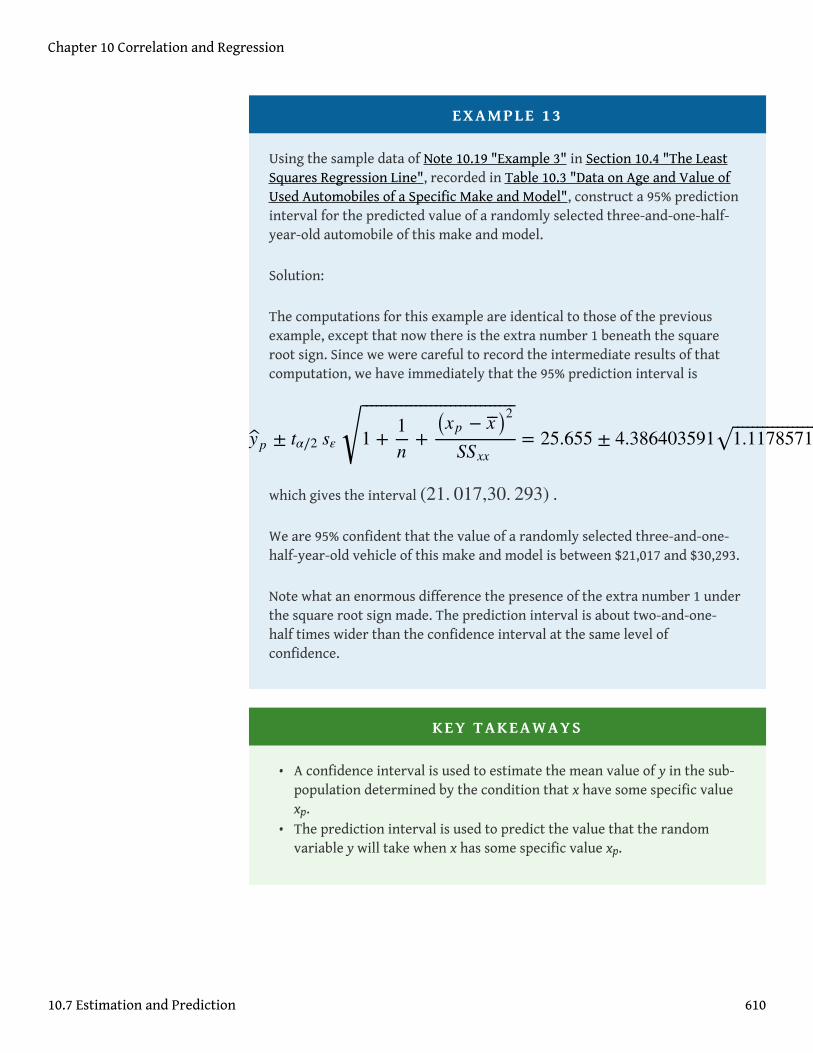
EXAMPLE 13
Using the sample data of Note 10.19 "Example 3" in Section 10.4 "The LeastSquares Regression Line", recorded in Table 10.3 "Data on Age and Value ofUsed Automobiles of a Specific Make and Model", construct a 95% predictioninterval for the predicted value of a randomly selected three-and-one-half-year-old automobile of this make and model.
Solution:
The computations for this example are identical to those of the previousexample, except that now there is the extra number 1 beneath the squareroot sign. Since we were careful to record the intermediate results of thatcomputation, we have immediately that the 95% prediction interval is
which gives the interval (21. 017,30. 293) .
We are 95% confident that the value of a randomly selected three-and-one-half-year-old vehicle of this make and model is between $21,017 and $30,293.
Note what an enormous difference the presence of the extra number 1 underthe square root sign made. The prediction interval is about two-and-one-half times wider than the confidence interval at the same level ofconfidence.
KEY TAKEAWAYS
• A confidence interval is used to estimate the mean value of y in the sub-population determined by the condition that x have some specific valuexp.
• The prediction interval is used to predict the value that the randomvariable y will take when x has some specific value xp.
yp ± tα∕2 sε 1 +1n
+ (xp − x⎯⎯)2SSxx
⎯ ⎯⎯⎯⎯⎯⎯⎯⎯⎯⎯⎯⎯⎯⎯⎯⎯⎯⎯⎯⎯⎯⎯⎯⎯⎯⎯⎯⎯⎯⎯
√ = 25.655 ± 4.386403591 1.1178571429⎯ ⎯⎯⎯⎯⎯⎯⎯⎯⎯⎯⎯⎯⎯⎯⎯⎯⎯⎯⎯⎯⎯⎯√ = 25.655 ± 4.638
Chapter 10 Correlation and Regression
10.7 Estimation and Prediction 610

EXERCISES
BASIC
For the Basic and Application exercises in this section use the computationsthat were done for the exercises with the same number in previous sections.
1. For the sample data set of Exercise 1 of Section 10.2 "The Linear CorrelationCoefficient"
a. Give a point estimate for the mean value of y in the sub-populationdetermined by the condition x = 4.
b. Construct the 90% confidence interval for that mean value.
2. For the sample data set of Exercise 2 of Section 10.2 "The Linear CorrelationCoefficient"
a. Give a point estimate for the mean value of y in the sub-populationdetermined by the condition x = 4.
b. Construct the 90% confidence interval for that mean value.
3. For the sample data set of Exercise 3 of Section 10.2 "The Linear CorrelationCoefficient"
a. Give a point estimate for the mean value of y in the sub-populationdetermined by the condition x = 7.
b. Construct the 95% confidence interval for that mean value.
4. For the sample data set of Exercise 4 of Section 10.2 "The Linear CorrelationCoefficient"
a. Give a point estimate for the mean value of y in the sub-populationdetermined by the condition x = 2.
b. Construct the 80% confidence interval for that mean value.
5. For the sample data set of Exercise 5 of Section 10.2 "The Linear CorrelationCoefficient"
a. Give a point estimate for the mean value of y in the sub-populationdetermined by the condition x = 1.
b. Construct the 80% confidence interval for that mean value.
6. For the sample data set of Exercise 6 of Section 10.2 "The Linear CorrelationCoefficient"
Chapter 10 Correlation and Regression
10.7 Estimation and Prediction 611
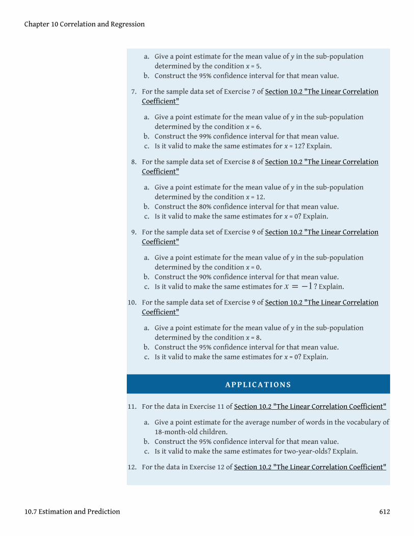
a. Give a point estimate for the mean value of y in the sub-populationdetermined by the condition x = 5.
b. Construct the 95% confidence interval for that mean value.
7. For the sample data set of Exercise 7 of Section 10.2 "The Linear CorrelationCoefficient"
a. Give a point estimate for the mean value of y in the sub-populationdetermined by the condition x = 6.
b. Construct the 99% confidence interval for that mean value.c. Is it valid to make the same estimates for x = 12? Explain.
8. For the sample data set of Exercise 8 of Section 10.2 "The Linear CorrelationCoefficient"
a. Give a point estimate for the mean value of y in the sub-populationdetermined by the condition x = 12.
b. Construct the 80% confidence interval for that mean value.c. Is it valid to make the same estimates for x = 0? Explain.
9. For the sample data set of Exercise 9 of Section 10.2 "The Linear CorrelationCoefficient"
a. Give a point estimate for the mean value of y in the sub-populationdetermined by the condition x = 0.
b. Construct the 90% confidence interval for that mean value.c. Is it valid to make the same estimates for x = −1? Explain.
10. For the sample data set of Exercise 9 of Section 10.2 "The Linear CorrelationCoefficient"
a. Give a point estimate for the mean value of y in the sub-populationdetermined by the condition x = 8.
b. Construct the 95% confidence interval for that mean value.c. Is it valid to make the same estimates for x = 0? Explain.
APPLICATIONS
11. For the data in Exercise 11 of Section 10.2 "The Linear Correlation Coefficient"
a. Give a point estimate for the average number of words in the vocabulary of18-month-old children.
b. Construct the 95% confidence interval for that mean value.c. Is it valid to make the same estimates for two-year-olds? Explain.
12. For the data in Exercise 12 of Section 10.2 "The Linear Correlation Coefficient"
Chapter 10 Correlation and Regression
10.7 Estimation and Prediction 612

a. Give a point estimate for the average braking distance of automobiles thatweigh 3,250 pounds.
b. Construct the 80% confidence interval for that mean value.c. Is it valid to make the same estimates for 5,000-pound automobiles?
Explain.
13. For the data in Exercise 13 of Section 10.2 "The Linear Correlation Coefficient"
a. Give a point estimate for the resting heart rate of a man who is 35 yearsold.
b. One of the men in the sample is 35 years old, but his resting heart rate isnot what you computed in part (a). Explain why this is not a contradiction.
c. Construct the 90% confidence interval for the mean resting heart rate ofall 35-year-old men.
14. For the data in Exercise 14 of Section 10.2 "The Linear Correlation Coefficient"
a. Give a point estimate for the wave height when the wind speed is 13 milesper hour.
b. One of the wind speeds in the sample is 13 miles per hour, but the height ofwaves that day is not what you computed in part (a). Explain why this isnot a contradiction.
c. Construct the 90% confidence interval for the mean wave height on dayswhen the wind speed is 13 miles per hour.
15. For the data in Exercise 15 of Section 10.2 "The Linear Correlation Coefficient"
a. The business owner intends to spend $2,500 on advertising next year. Givean estimate of next year’s revenue based on this fact.
b. Construct the 90% prediction interval for next year’s revenue, based on theintent to spend $2,500 on advertising.
16. For the data in Exercise 16 of Section 10.2 "The Linear Correlation Coefficient"
a. A two-year-old girl is 32.3 inches long. Predict her adult height.b. Construct the 95% prediction interval for the girl’s adult height.
17. For the data in Exercise 17 of Section 10.2 "The Linear Correlation Coefficient"
a. Lodovico has a 78.6 average in his physics class just before the final. Give apoint estimate of what his final exam grade will be.
b. Explain whether an interval estimate for this problem is a confidenceinterval or a prediction interval.
c. Based on your answer to (b), construct an interval estimate for Lodovico’sfinal exam grade at the 90% level of confidence.
18. For the data in Exercise 18 of Section 10.2 "The Linear Correlation Coefficient"
Chapter 10 Correlation and Regression
10.7 Estimation and Prediction 613
a. This year 86.2 million acres of corn were planted. Give a point estimate ofthe number of acres that will be harvested this year.
b. Explain whether an interval estimate for this problem is a confidenceinterval or a prediction interval.
c. Based on your answer to (b), construct an interval estimate for the numberof acres that will be harvested this year, at the 99% level of confidence.
19. For the data in Exercise 19 of Section 10.2 "The Linear Correlation Coefficient"
a. Give a point estimate for the blood concentration of the active ingredientof this medication in a man who has consumed 1.5 ounces of themedication just recently.
b. Gratiano just consumed 1.5 ounces of this medication 30 minutes ago.Construct a 95% prediction interval for the concentration of the activeingredient in his blood right now.
20. For the data in Exercise 20 of Section 10.2 "The Linear Correlation Coefficient"
a. You measure the girth of a free-standing oak tree five feet off the groundand obtain the value 127 inches. How old do you estimate the tree to be?
b. Construct a 90% prediction interval for the age of this tree.
21. For the data in Exercise 21 of Section 10.2 "The Linear Correlation Coefficient"
a. A test cylinder of concrete three days old fails at 1,750 psi. Predict what the28-day strength of the concrete will be.
b. Construct a 99% prediction interval for the 28-day strength of thisconcrete.
c. Based on your answer to (b), what would be the minimum 28-day strengthyou could expect this concrete to exhibit?
22. For the data in Exercise 22 of Section 10.2 "The Linear Correlation Coefficient"
a. Tomorrow’s average temperature is forecast to be 53 degrees. Estimate theenergy demand tomorrow.
b. Construct a 99% prediction interval for the energy demand tomorrow.c. Based on your answer to (b), what would be the minimum demand you
could expect?
LARGE DATA SET EXERCISES
23. Large Data Set 1 lists the SAT scores and GPAs of 1,000 students.
http://www.gone.2012books.lardbucket.org/sites/all/files/data1.xls
Chapter 10 Correlation and Regression
10.7 Estimation and Prediction 614
a. Give a point estimate of the mean GPA of all students who score 1350 onthe SAT.
b. Construct a 90% confidence interval for the mean GPA of all students whoscore 1350 on the SAT.
24. Large Data Set 12 lists the golf scores on one round of golf for 75 golfers firstusing their own original clubs, then using clubs of a new, experimental design(after two months of familiarization with the new clubs).
http://www.gone.2012books.lardbucket.org/sites/all/files/data12.xls
a. Thurio averages 72 strokes per round with his own clubs. Give a pointestimate for his score on one round if he switches to the new clubs.
b. Explain whether an interval estimate for this problem is a confidenceinterval or a prediction interval.
c. Based on your answer to (b), construct an interval estimate for Thurio’sscore on one round if he switches to the new clubs, at 90% confidence.
25. Large Data Set 13 records the number of bidders and sales price of a particulartype of antique grandfather clock at 60 auctions.
http://www.gone.2012books.lardbucket.org/sites/all/files/data13.xls
a. There are seven likely bidders at the Verona auction today. Give a pointestimate for the price of such a clock at today’s auction.
b. Explain whether an interval estimate for this problem is a confidenceinterval or a prediction interval.
c. Based on your answer to (b), construct an interval estimate for the likelysale price of such a clock at today’s sale, at 95% confidence.
Chapter 10 Correlation and Regression
10.7 Estimation and Prediction 615
ANSWERS
1. a. 5.647,b. 5.647 ± 1.253
3. a. −0.188,b. −0.188 ± 3.041
5. a. 1.875,b. 1.875 ± 1.423
7. a. 5.4,b. 5.4 ± 3.355 ,c. invalid (extrapolation)
9. a. 2.4,b. 2.4 ± 1.474 ,c. valid (−1 is in the range of the x-values in the data set)
11. a. 31.3 words,b. 31.3 ± 7.1 words,c. not valid, since two years is 24 months, hence this is extrapolation
13. a. 73.2 beats/min,b. The man’s heart rate is not the predicted average for all men his age. c.
73.2 ± 1.2 beats/min
15. a. $224,562,b. $224,562 ± $28,699
17. a. 74,b. Prediction (one person, not an average for all who have average 78.6
before the final exam),c. 74 ± 24
19. a. 0.066%,b. 0.066 ± 0.034%
21. a. 4,656 psi,b. 4,656 ± 321 psi,c. 4,656 − 321 = 4,335 psi
23. a. 2.19
b. (2. 1421,2. 2316)25. a. 7771.39
b. A prediction interval.
Chapter 10 Correlation and Regression
10.7 Estimation and Prediction 616
c. (7410. 41,8132. 38)
Chapter 10 Correlation and Regression
10.7 Estimation and Prediction 617
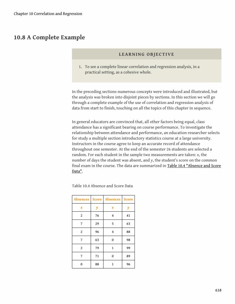
10.8 A Complete Example
LEARNING OBJECTIVE
1. To see a complete linear correlation and regression analysis, in apractical setting, as a cohesive whole.
In the preceding sections numerous concepts were introduced and illustrated, butthe analysis was broken into disjoint pieces by sections. In this section we will gothrough a complete example of the use of correlation and regression analysis ofdata from start to finish, touching on all the topics of this chapter in sequence.
In general educators are convinced that, all other factors being equal, classattendance has a significant bearing on course performance. To investigate therelationship between attendance and performance, an education researcher selectsfor study a multiple section introductory statistics course at a large university.Instructors in the course agree to keep an accurate record of attendancethroughout one semester. At the end of the semester 26 students are selected arandom. For each student in the sample two measurements are taken: x, thenumber of days the student was absent, and y, the student’s score on the commonfinal exam in the course. The data are summarized in Table 10.4 "Absence and ScoreData".
Table 10.4 Absence and Score Data
Absences Score Absences Score
x y x y
2 76 4 41
7 29 5 63
2 96 4 88
7 63 0 98
2 79 1 99
7 71 0 89
0 88 1 96
Chapter 10 Correlation and Regression
618
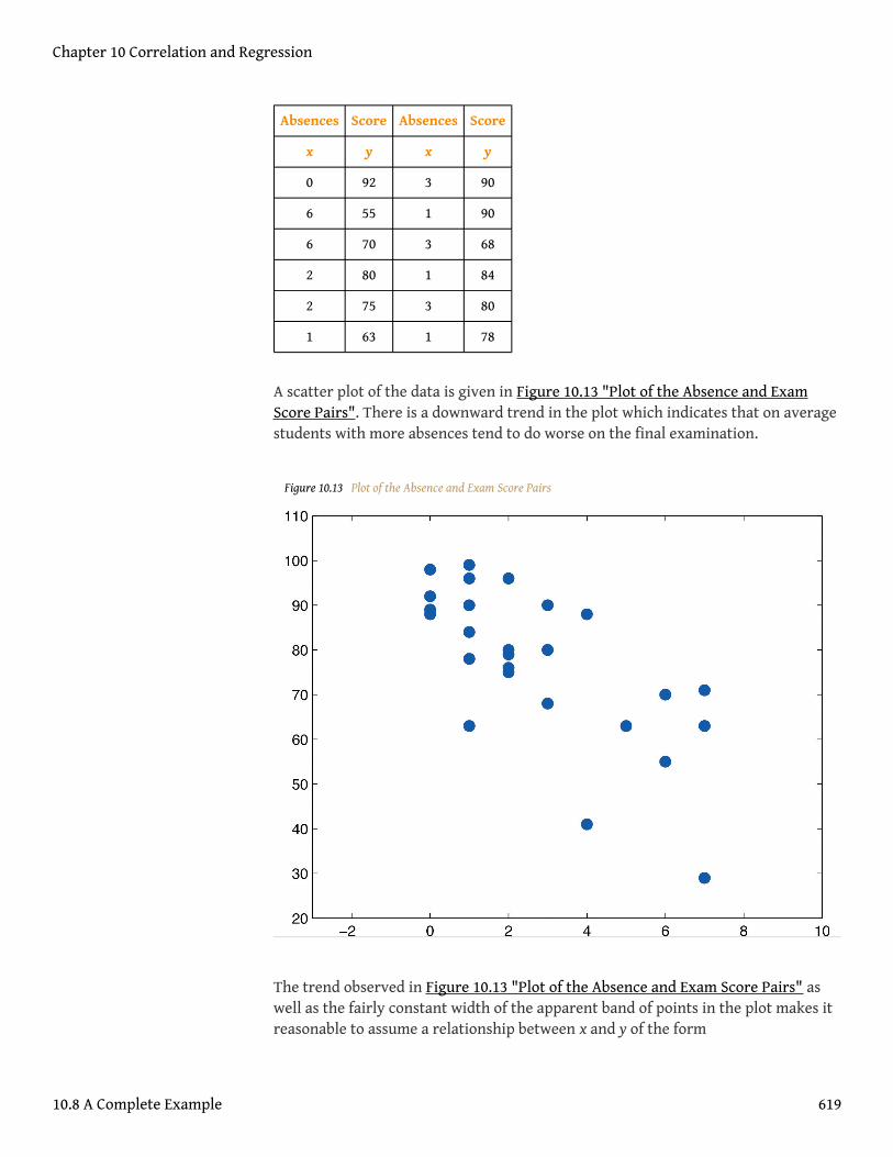
Absences Score Absences Score
x y x y
0 92 3 90
6 55 1 90
6 70 3 68
2 80 1 84
2 75 3 80
1 63 1 78
A scatter plot of the data is given in Figure 10.13 "Plot of the Absence and ExamScore Pairs". There is a downward trend in the plot which indicates that on averagestudents with more absences tend to do worse on the final examination.
Figure 10.13 Plot of the Absence and Exam Score Pairs
The trend observed in Figure 10.13 "Plot of the Absence and Exam Score Pairs" aswell as the fairly constant width of the apparent band of points in the plot makes itreasonable to assume a relationship between x and y of the form
Chapter 10 Correlation and Regression
10.8 A Complete Example 619
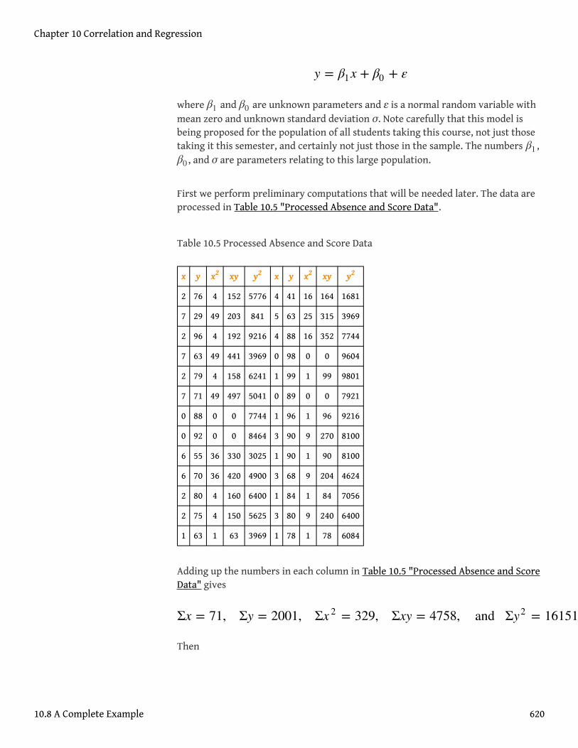
where β1 and β0 are unknown parameters and ε is a normal random variable withmean zero and unknown standard deviation σ. Note carefully that this model isbeing proposed for the population of all students taking this course, not just thosetaking it this semester, and certainly not just those in the sample. The numbers β1 ,β0 , and σ are parameters relating to this large population.
First we perform preliminary computations that will be needed later. The data areprocessed in Table 10.5 "Processed Absence and Score Data".
Table 10.5 Processed Absence and Score Data
x y x2 xy y2 x y x2 xy y2
2 76 4 152 5776 4 41 16 164 1681
7 29 49 203 841 5 63 25 315 3969
2 96 4 192 9216 4 88 16 352 7744
7 63 49 441 3969 0 98 0 0 9604
2 79 4 158 6241 1 99 1 99 9801
7 71 49 497 5041 0 89 0 0 7921
0 88 0 0 7744 1 96 1 96 9216
0 92 0 0 8464 3 90 9 270 8100
6 55 36 330 3025 1 90 1 90 8100
6 70 36 420 4900 3 68 9 204 4624
2 80 4 160 6400 1 84 1 84 7056
2 75 4 150 5625 3 80 9 240 6400
1 63 1 63 3969 1 78 1 78 6084
Adding up the numbers in each column in Table 10.5 "Processed Absence and ScoreData" gives
Then
y = β1x + β0 + ε
Σx = 71, Σy = 2001, Σx 2 = 329, Σxy = 4758, and Σy2 = 161511.
Chapter 10 Correlation and Regression
10.8 A Complete Example 620

and
We begin the actual modelling by finding the least squares regression line, the linethat best fits the data. Its slope and y-intercept are
Rounding these numbers to two decimal places, the least squares regression line forthese data is
The goodness of fit of this line to the scatter plot, the sum of its squared errors, is
This number is not particularly informative in itself, but we use it to compute theimportant statistic
The statistic sε estimates the standard deviation σ of the normal random variable εin the model. Its meaning is that among all students with the same number ofabsences, the standard deviation of their scores on the final exam is about 12.1points. Such a large value on a 100-point exam means that the final exam scores of
SSxx
SSxy
SSyy
=
=
=
Σx 2 −1n
(Σx)2 = 329 −126
(71)2 = 135.1153846
Σxy −1n
(Σx) (Σy) = 4758 −126
(71) (2001) = −706.2692308
Σy2 −1n (Σy) 2 = 161511 −
126
(2001) 2 = 7510.961538
x⎯⎯ =Σxn
=7126
= 2.730769231 and y⎯⎯ =Σyn
=200126
= 76.96153846
β 1
β 0
=
=
SSxy
SSxx=
−706.2692308135.1153846
= −5.227156278
y⎯⎯ − β 1x⎯⎯ = 76.96153846 − (−5.227156278) (2.730769231) = 91.23569553
y = −5.23 x + 91.24.
SSE = SSyy − β 1SSxy = 7510.961538 − (−5.227156278) (−706.2692308) = 3819.181894
sε =SSE
n−2
⎯ ⎯⎯⎯⎯⎯⎯⎯
√ =3819.181894
24
⎯ ⎯⎯⎯⎯⎯⎯⎯⎯⎯⎯⎯⎯⎯⎯⎯⎯⎯⎯⎯⎯⎯⎯
√ = 12.11988495
Chapter 10 Correlation and Regression
10.8 A Complete Example 621
each sub-population of students, based on the number of absences, are highlyvariable.
The size and sign of the slope β 1 = −5.23 indicate that, for every class missed,students tend to score about 5.23 fewer points lower on the final exam on average.Similarly for every two classes missed students tend to score on average2 × 5.23 = 10.46 fewer points on the final exam, or about a letter grade worse onaverage.
Since 0 is in the range of x-values in the data set, the y-intercept also has meaningin this problem. It is an estimate of the average grade on the final exam of allstudents who have perfect attendance. The predicted average of such students isβ 0 = 91.24.
Before we use the regression equation further, or perform other analyses, it wouldbe a good idea to examine the utility of the linear regression model. We can do thisin two ways: 1) by computing the correlation coefficient r to see how strongly thenumber of absences x and the score y on the final exam are correlated, and 2) bytesting the null hypothesis H0 : β1 = 0 (the slope of the population regression lineis zero, so x is not a good predictor of y) against the natural alternative Ha : β1 < 0(the slope of the population regression line is negative, so final exam scores y godown as absences x go up).
The correlation coefficient r is
a moderate negative correlation.
Turning to the test of hypotheses, let us test at the commonly used 5% level ofsignificance. The test is
r =SSxy
SSxx SSyy⎯ ⎯⎯⎯⎯⎯⎯⎯⎯⎯⎯⎯⎯⎯⎯
√=
−706.2692308
(135.1153846) (7510.961538)⎯ ⎯⎯⎯⎯⎯⎯⎯⎯⎯⎯⎯⎯⎯⎯⎯⎯⎯⎯⎯⎯⎯⎯⎯⎯⎯⎯⎯⎯⎯⎯⎯⎯⎯⎯⎯⎯⎯⎯⎯⎯⎯⎯⎯⎯⎯⎯⎯⎯⎯√= −0.7010840977
H0 : β1 = 0vs. Ha : β1 < 0 @α = 0.05
Chapter 10 Correlation and Regression
10.8 A Complete Example 622
From Figure 12.3 "Critical Values of ", with df = 26 − 2 = 24degrees of freedomt0.05 = 1.711, so the rejection region is (−∞, −1.711] . The value of thestandardized test statistic is
which falls in the rejection region. We reject H0 in favor of Ha. The data provide
sufficient evidence, at the 5% level of significance, to conclude that β1 is negative,meaning that as the number of absences increases average score on the final examdecreases.
As already noted, the value β1 = −5.23 gives a point estimate of how much oneadditional absence is reflected in the average score on the final exam. For eachadditional absence the average drops by about 5.23 points. We can widen this pointestimate to a confidence interval for β1 . At the 95% confidence level, from Figure12.3 "Critical Values of " with df = 26 − 2 = 24degrees of freedom,tα∕2 = t0.025 = 2.064.The 95% confidence interval for β1 based on our sample datais
or (−7.38, −3.08) .We are 95% confident that, among all students who ever takethis course, for each additional class missed the average score on the final examgoes down by between 3.08 and 7.38 points.
If we restrict attention to the sub-population of all students who have exactly fiveabsences, say, then using the least squares regression equationy = −5.23x + 91.24 we estimate that the average score on the final exam forthose students is
This is also our best guess as to the score on the final exam of any particular studentwho is absent five times. A 95% confidence interval for the average score on thefinal exam for all students with five absences is
t =β 1 − B0
sε / SSxx⎯ ⎯⎯⎯⎯⎯⎯⎯
√=
−5.227156278 − 0
12.11988495 / 135.1153846⎯ ⎯⎯⎯⎯⎯⎯⎯⎯⎯⎯⎯⎯⎯⎯⎯⎯⎯⎯⎯⎯
√= −5.013
β 1 ± tα∕2sε
SSxx⎯ ⎯⎯⎯⎯⎯⎯⎯
√= −5.23 ± 2.064
12.11988495
135.1153846⎯ ⎯⎯⎯⎯⎯⎯⎯⎯⎯⎯⎯⎯⎯⎯⎯⎯⎯⎯⎯⎯
√= −5.23 ± 2.15
y = −5.23 (5) + 91.24 = 65.09
Chapter 10 Correlation and Regression
10.8 A Complete Example 623
which is the interval (58. 17,72. 01) .This confidence interval suggests that thetrue mean score on the final exam for all students who are absent from class exactlyfive times during the semester is likely to be between 58.17 and 72.01.
If a particular student misses exactly five classes during the semester, his score onthe final exam is predicted with 95% confidence to be in the interval
which is the interval (39. 13,91. 05) .This prediction interval suggests that thisindividual student’s final exam score is likely to be between 39.13 and 91.05.Whereas the 95% confidence interval for the average score of all student with fiveabsences gave real information, this interval is so wide that it says practicallynothing about what the individual student’s final exam score might be. This is anexample of the dramatic effect that the presence of the extra summand 1 under thesquare sign in the prediction interval can have.
Finally, the proportion of the variability in the scores of students on the final examthat is explained by the linear relationship between that score and the number ofabsences is estimated by the coefficient of determination, r2. Since we have alreadycomputed r above we easily find that
or about 49%. Thus although there is a significant correlation between attendanceand performance on the final exam, and we can estimate with fair accuracy theaverage score of students who miss a certain number of classes, nevertheless lessthan half the total variation of the exam scores in the sample is explained by thenumber of absences. This should not come as a surprise, since there are manyfactors besides attendance that bear on student performance on exams.
yp ± tα∕2sε1n
+ (xp − x⎯⎯)2SSxx
⎯ ⎯⎯⎯⎯⎯⎯⎯⎯⎯⎯⎯⎯⎯⎯⎯⎯⎯⎯⎯⎯⎯⎯⎯
√ =
==
65.09 ± (2.064) (12.11988495) 126
+ (5 − 2.730769231) 2
135.1153846
⎯ ⎯⎯⎯⎯⎯⎯⎯⎯⎯⎯⎯⎯⎯⎯⎯⎯⎯⎯⎯⎯⎯⎯⎯⎯⎯⎯⎯⎯⎯⎯⎯⎯⎯⎯⎯⎯⎯⎯⎯⎯⎯⎯
√65.09 ± 25.01544254 0.0765727299⎯ ⎯⎯⎯⎯⎯⎯⎯⎯⎯⎯⎯⎯⎯⎯⎯⎯⎯⎯⎯⎯⎯⎯
√65.09 ± 6.92
yp ± tα∕2sε 1 +1n
+ (xp − x⎯⎯)2SSxx
⎯ ⎯⎯⎯⎯⎯⎯⎯⎯⎯⎯⎯⎯⎯⎯⎯⎯⎯⎯⎯⎯⎯⎯⎯⎯⎯⎯⎯⎯⎯⎯
√ =
=
65.09 ± 25.01544254 1.0765727299⎯ ⎯⎯⎯⎯⎯⎯⎯⎯⎯⎯⎯⎯⎯⎯⎯⎯⎯⎯⎯⎯⎯⎯√
65.09 ± 25.96
r2 = (−0.7010840977) 2 = 0.491518912
Chapter 10 Correlation and Regression
10.8 A Complete Example 624
KEY TAKEAWAY
• It is a good idea to attend class.
Chapter 10 Correlation and Regression
10.8 A Complete Example 625

EXERCISES
The exercises in this section are unrelated to those in previous sections.
1. The data give the amount x of silicofluoride in the water (mg/L) and theamount y of lead in the bloodstream (μg/dL) of ten children in variouscommunities with and without municipal water. Perform a complete analysisof the data, in analogy with the discussion in this section (that is, make ascatter plot, do preliminary computations, find the least squares regressionline, find SSE , sε , and r, and so on). In the hypothesis test use as thealternative hypothesis β1 > 0, and test at the 5% level of significance. Useconfidence level 95% for the confidence interval for β1 . Construct 95%confidence and predictions intervals at xp = 2 at the end.
2. The table gives the weight x (thousands of pounds) and available heat energy y(million BTU) of a standard cord of various species of wood typically used forheating. Perform a complete analysis of the data, in analogy with thediscussion in this section (that is, make a scatter plot, do preliminarycomputations, find the least squares regression line, find SSE , sε , and r, andso on). In the hypothesis test use as the alternative hypothesis β1 > 0, andtest at the 5% level of significance. Use confidence level 95% for the confidenceinterval for β1 . Construct 95% confidence and predictions intervals atxp = 5 at the end.
LARGE DATA SET EXERCISES
3. Large Data Sets 3 and 3A list the shoe sizes and heights of 174 customersentering a shoe store. The gender of the customer is not indicated in LargeData Set 3. However, men’s and women’s shoes are not measured on the samescale; for example, a size 8 shoe for men is not the same size as a size 8 shoe for
x
y
0.00.3
0.00.1
1.14.7
1.43.2
1.65.1
x
y
1.77.0
2.05.0
2.06.1
2.28.6
2.29.5
x
y
3.3723.6
3.5017.5
4.2920.1
4.0021.6
4.6428.1
x
y
4.9925.3
4.9427.0
5.4830.7
3.2618.9
4.1620.7
Chapter 10 Correlation and Regression
10.8 A Complete Example 626
women. Thus it would not be meaningful to apply regression analysis to LargeData Set 3. Nevertheless, compute the scatter diagrams, with shoe size as theindependent variable (x) and height as the dependent variable (y), for (i) justthe data on men, (ii) just the data on women, and (iii) the full mixed data setwith both men and women. Does the third, invalid scatter diagram lookmarkedly different from the other two?
http://www.gone.2012books.lardbucket.org/sites/all/files/data3.xls
http://www.gone.2012books.lardbucket.org/sites/all/files/data3A.xls
4. Separate out from Large Data Set 3A just the data on men and do a completeanalysis, with shoe size as the independent variable (x) and height as thedependent variable (y). Use α = 0.05 and xp = 10 whenever appropriate.
http://www.gone.2012books.lardbucket.org/sites/all/files/data3A.xls
5. Separate out from Large Data Set 3A just the data on women and do a completeanalysis, with shoe size as the independent variable (x) and height as thedependent variable (y). Use α = 0.05 and xp = 10 whenever appropriate.
http://www.gone.2012books.lardbucket.org/sites/all/files/data3A.xls
Chapter 10 Correlation and Regression
10.8 A Complete Example 627
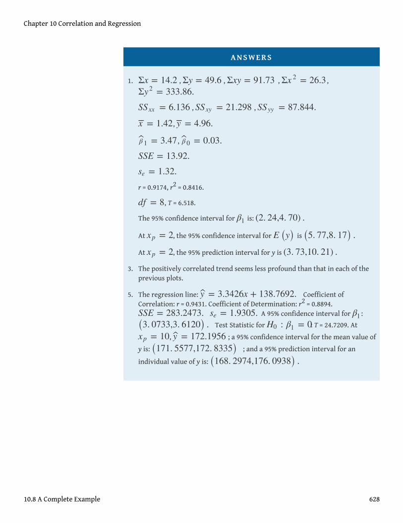
ANSWERS
1. Σx = 14.2 , Σy = 49.6 , Σxy = 91.73 , Σx 2 = 26.3 ,
Σy2 = 333.86.SSxx = 6.136 , SSxy = 21.298 , SSyy = 87.844.
x⎯⎯ = 1.42, y⎯⎯ = 4.96.
β 1 = 3.47 , β 0 = 0.03.SSE = 13.92.sε = 1.32.r = 0.9174, r2 = 0.8416.
df = 8, T = 6.518.
The 95% confidence interval for β1 is: (2. 24,4. 70) .
At xp = 2, the 95% confidence interval for E (y) is (5. 77,8. 17) .At xp = 2, the 95% prediction interval for y is (3. 73,10. 21) .
3. The positively correlated trend seems less profound than that in each of theprevious plots.
5. The regression line: y = 3.3426x + 138.7692. Coefficient ofCorrelation: r = 0.9431. Coefficient of Determination: r2 = 0.8894.SSE = 283.2473. se = 1.9305. A 95% confidence interval for β1 :
(3. 0733,3. 6120) . Test Statistic for H0 : β1 = 0: T = 24.7209. At
xp = 10, y = 172.1956 ; a 95% confidence interval for the mean value of
y is: (171. 5577,172. 8335) ; and a 95% prediction interval for an
individual value of y is: (168. 2974,176. 0938) .
Chapter 10 Correlation and Regression
10.8 A Complete Example 628
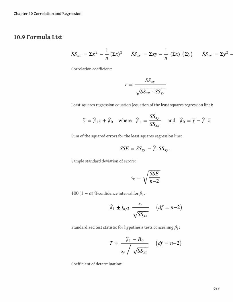
10.9 Formula List
Correlation coefficient:
Least squares regression equation (equation of the least squares regression line):
Sum of the squared errors for the least squares regression line:
Sample standard deviation of errors:
100 (1 − α)%confidence interval for β1 :
Standardized test statistic for hypothesis tests concerning β1 :
Coefficient of determination:
SSxx = Σx 2 −1n
(Σx)2 SSxy = Σxy −1n
(Σx) (Σy) SSyy = Σy2 −1n (Σy) 2
r =SSxy
SSxx · SSyy⎯ ⎯⎯⎯⎯⎯⎯⎯⎯⎯⎯⎯⎯⎯⎯⎯⎯⎯
√
y = β 1x + β 0 where β 1 =SSxy
SSxxand β 0 = y⎯⎯ − β 1x
⎯⎯
SSE = SSyy − β 1SSxy .
sε =SSE
n−2
⎯ ⎯⎯⎯⎯⎯⎯⎯
√
β 1 ± tα∕2sε
SSxx⎯ ⎯⎯⎯⎯⎯⎯⎯
√(df = n−2)
T =β 1 − B0
sε / SSxx⎯ ⎯⎯⎯⎯⎯⎯⎯
√(df = n−2)
Chapter 10 Correlation and Regression
629
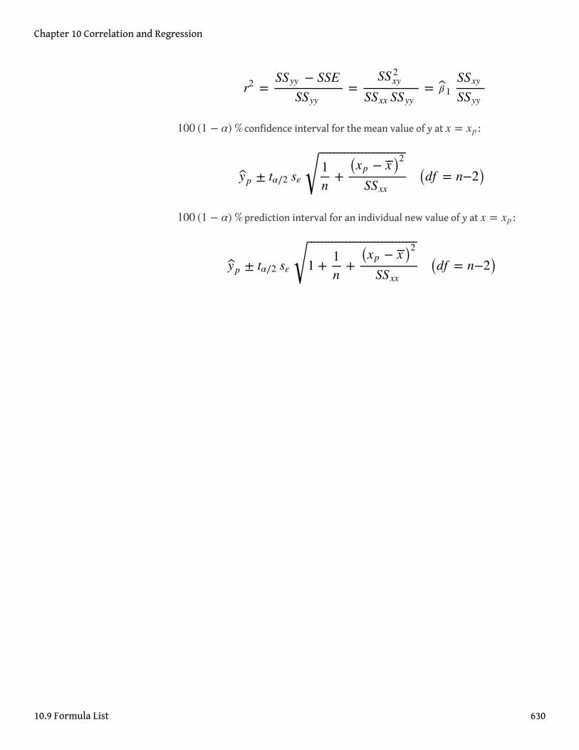
100 (1 − α)%confidence interval for the mean value of y at x = xp :
100 (1 − α)%prediction interval for an individual new value of y at x = xp :
r2 =SSyy − SSE
SSyy=
SS 2xy
SSxx SSyy= β 1
SSxy
SSyy
yp ± tα∕2 sε1n
+ (xp − x⎯⎯)2SSxx
⎯ ⎯⎯⎯⎯⎯⎯⎯⎯⎯⎯⎯⎯⎯⎯⎯⎯⎯⎯⎯⎯⎯⎯⎯
√ (df = n−2)
yp ± tα∕2 sε 1 +1n
+ (xp − x⎯⎯)2SSxx
⎯ ⎯⎯⎯⎯⎯⎯⎯⎯⎯⎯⎯⎯⎯⎯⎯⎯⎯⎯⎯⎯⎯⎯⎯⎯⎯⎯⎯⎯⎯⎯
√ (df = n−2)
Chapter 10 Correlation and Regression
10.9 Formula List 630
Related Documents