Chapter 1: Market Indexes, Financial Time Series and their Characteristics • What is time series (TS) analysis? Observe the following two data sets: Hang Seng 12877 12850 13023 ··· Index Date 30.8.04 31.8.04 01.9.04 ··· Student’s 130kg 200kg 45kg ··· Weights Students A B C ··· What is the difference between these two data sets? • Definition: A time series (TS) is a sequence of random variables labeled by time t. Time series data are observations of TS. 1

Welcome message from author
This document is posted to help you gain knowledge. Please leave a comment to let me know what you think about it! Share it to your friends and learn new things together.
Transcript
Chapter 1: Market Indexes, Financial Time
Series and their Characteristics
• What is time series (TS) analysis?
Observe the following two data sets:
Hang Seng 12877 12850 13023 · · ·IndexDate 30.8.04 31.8.04 01.9.04 · · ·
Student’s 130kg 200kg 45kg · · ·WeightsStudents A B C · · ·
What is the difference between these two data
sets?
• Definition:
A time series (TS) is a sequence of random
variables labeled by time t.
Time series data are observations of TS.
1
TSA History
• Linear TSA: The beginning/babyhood 1927
• George Udny Yule (1871-1951), a British statis-
tician.
• Eugen Slutsky (1880-1948), a Russian/Soviet
mathematical statistician, economist and po-
litical economist.
• Herman Ole Andreas Wold ( 1908– 1992)
• Peter Whittle (1927-) (ARMA model)
• Linear TSA in 1970’s
• George Edward Pelham Box (1919–2013), a
British statistician (quality control, TSA, de-
sign of experiments, and Bayesian inference).
He has been called “one of the great statistical
minds of the 20th century”.
• Sir Ronald Aylmer Fisher (1890 –1962)
• Box & Jenkins (1976) Time Series Analysis:
Forecasting and Control

• Nonlinear TSA in 1950’s
• Patrick Alfred Pierce Moran (1917–1988), an
Australian statistician (probability theory, pop-
ulation and evolutionary genetics).
• Peter Whittle (1927-, New Zealand), stochas-
tic nets, optimal control, time series analysis,
stochastic optimisation and stochastic dynam-
ics.
• Nonlinear TSA in 1980’s
• Howell Tong (1944–, in Hong Kong) (TAR
model).
• Robert Fry Engle III (1942–) is an American
economist and the winner of the 2003 Nobel
Memorial Prize.
• What is financial time series (FTS)?
Examples
1. Daily log returns of Hang Sang Index .
2. Monthly log return of exchange rates of
Japan-USA.
3. China life daily stock data.
4. HSBC daily stock data.
0 2000 4000 6000 8000
020
0040
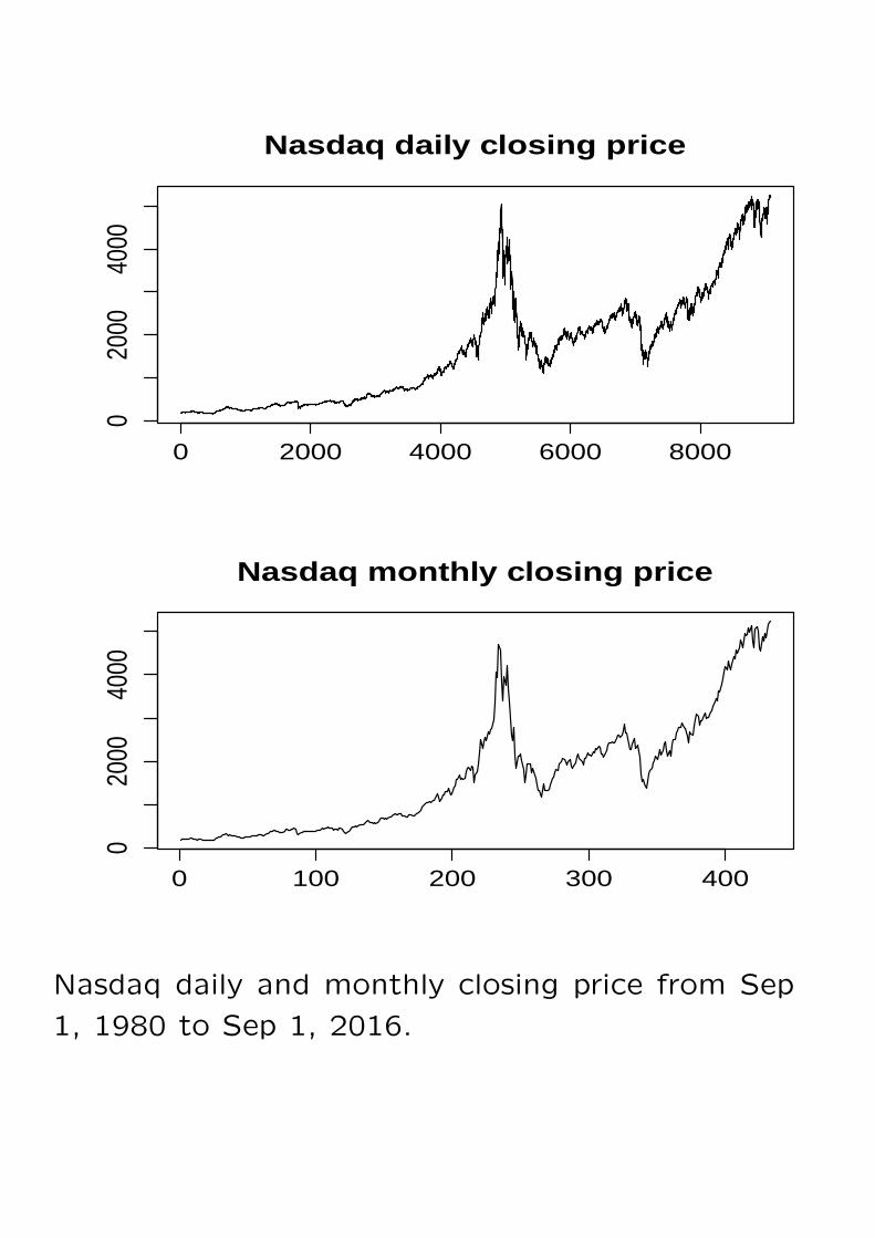
00Nasdaq daily closing price
0 100 200 300 400
020
0040
00
Nasdaq monthly closing price
Nasdaq daily and monthly closing price from Sep
1, 1980 to Sep 1, 2016.
Special features of FTS
1. Theory and practice of asset valuation over
time.
2. Added more uncertainty. For example, FTS
must deal with the changing business and eco-
nomic environment and the fact that volatility is
not directly observed.
General objective of the course
to provide some basic knowledge of financial time
series data
to introduce some statistical tools and economet-
ric models useful for analyzing these series.
to gain empirical experience in analyzing FTS
to study methods for assessing market risk
to analyze high-dimensional asset returns.
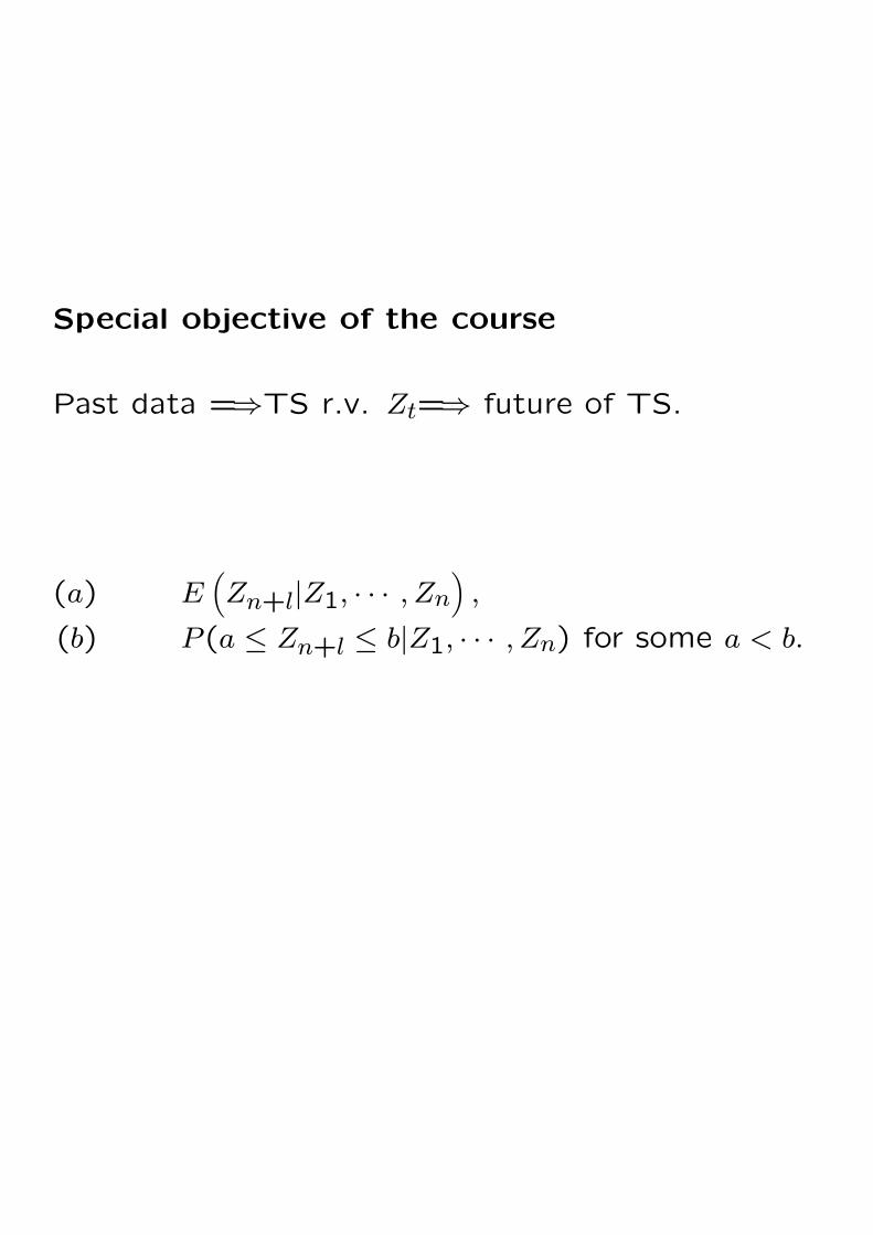
Special objective of the course
Past data =⇒TS r.v. Zt=⇒ future of TS.
(a) E(Zn+l|Z1, · · · , Zn
),
(b) P (a ≤ Zn+l ≤ b|Z1, · · · , Zn) for some a < b.
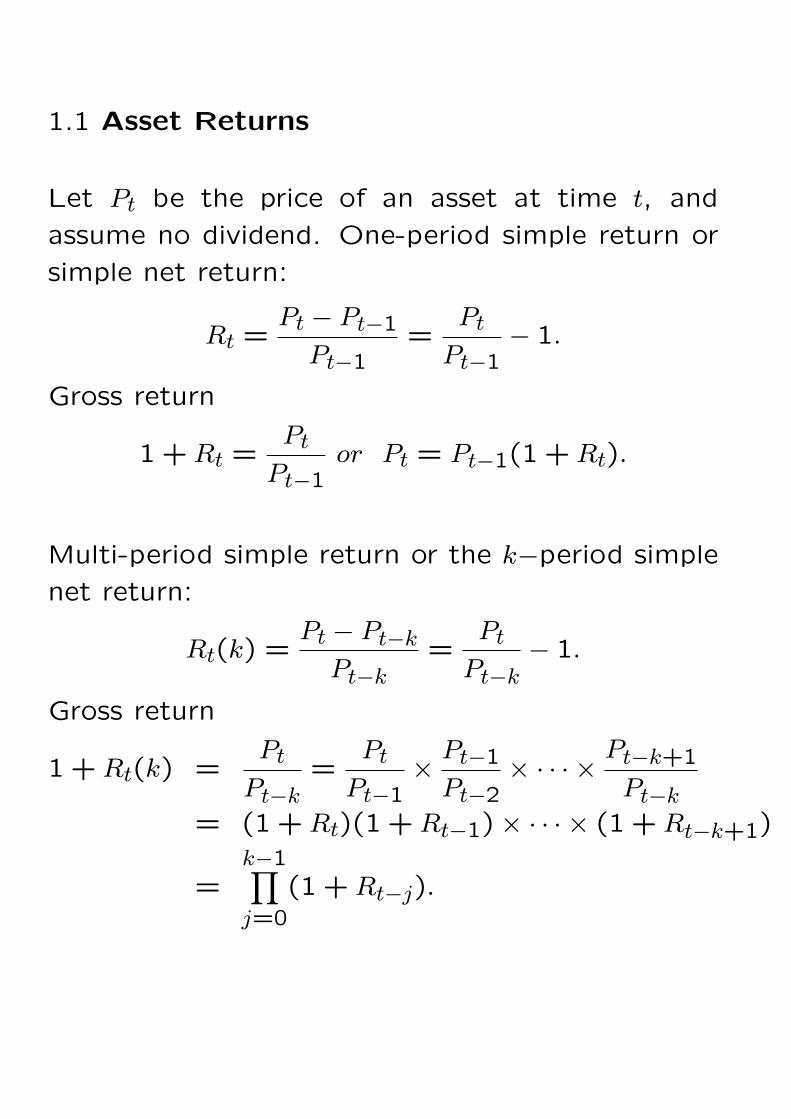
1.1 Asset Returns
Let Pt be the price of an asset at time t, and
assume no dividend. One-period simple return or
simple net return:
Rt =Pt − Pt−1
Pt−1=
Pt
Pt−1− 1.
Gross return
1 +Rt =Pt
Pt−1or Pt = Pt−1(1 +Rt).
Multi-period simple return or the k−period simple
net return:
Rt(k) =Pt − Pt−k
Pt−k=
Pt
Pt−k− 1.
Gross return
1 +Rt(k) =Pt
Pt−k=
Pt
Pt−1×
Pt−1
Pt−2× · · · ×
Pt−k+1
Pt−k
= (1+Rt)(1 +Rt−1)× · · · × (1 +Rt−k+1)
=k−1∏j=0
(1 +Rt−j).
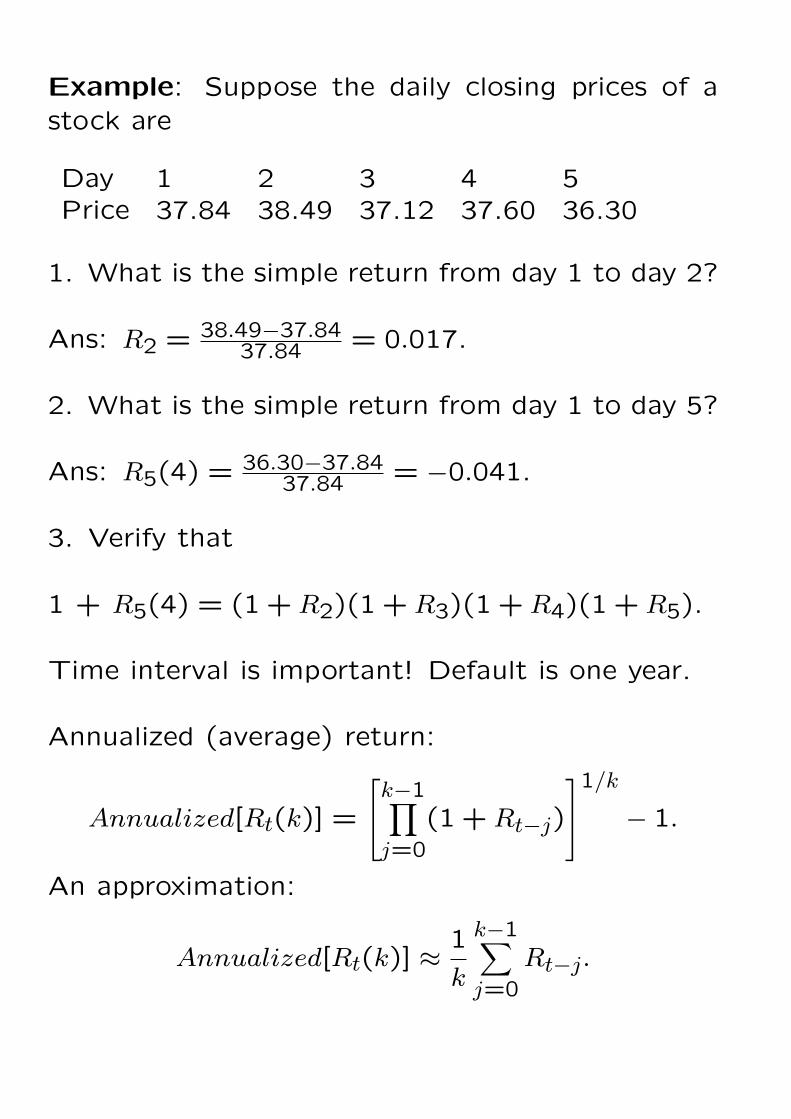
Example: Suppose the daily closing prices of astock are
Day 1 2 3 4 5Price 37.84 38.49 37.12 37.60 36.30
1. What is the simple return from day 1 to day 2?
Ans: R2 = 38.49−37.8437.84 = 0.017.
2. What is the simple return from day 1 to day 5?
Ans: R5(4) = 36.30−37.8437.84 = −0.041.
3. Verify that
1 + R5(4) = (1+R2)(1 +R3)(1 +R4)(1 +R5).
Time interval is important! Default is one year.
Annualized (average) return:
Annualized[Rt(k)] =
k−1∏j=0
(1 +Rt−j)
1/k − 1.
An approximation:
Annualized[Rt(k)] ≈1
k
k−1∑j=0
Rt−j.
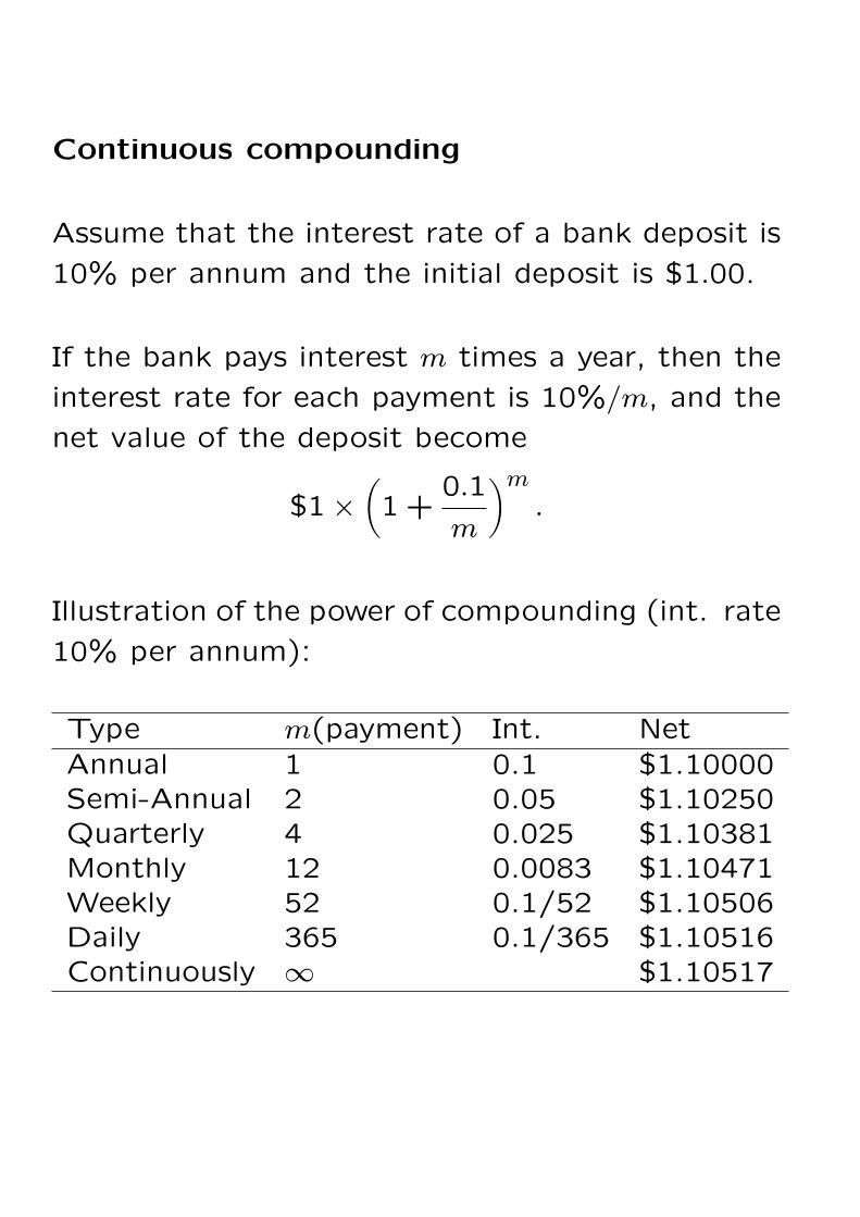
Continuous compounding
Assume that the interest rate of a bank deposit is
10% per annum and the initial deposit is $1.00.
If the bank pays interest m times a year, then the
interest rate for each payment is 10%/m, and the
net value of the deposit become
$1×(1+
0.1
m
)m.
Illustration of the power of compounding (int. rate
10% per annum):
Type m(payment) Int. NetAnnual 1 0.1 $1.10000Semi-Annual 2 0.05 $1.10250Quarterly 4 0.025 $1.10381Monthly 12 0.0083 $1.10471Weekly 52 0.1/52 $1.10506Daily 365 0.1/365 $1.10516Continuously ∞ $1.10517
In general, the net asset value A of the continuous
compounding is
A = C exp(r × n),
r is the interest rate per annum, C is the initial
capital, n is the number of years, and and exp is
the exponential function.
Present value:
C = A exp[−r × n].
Continuously compounded (or log) return
rt = ln(1 +Rt) = lnPt
Pt−1= pt − pt−1,
where pt = ln(Pt)
Multi-period log return:
rt(k) = ln[1 +Rt(k)]
= ln[(1 +Rt)(1 +Rt−1)(1 +Rt−k+1)]
= ln(1 +Rt) + ln(1 +Rt−1)
+ · · ·+ ln(1 +Rt−k+1)
= rt + rt−1 + · · ·+ rt−k+1.
Example (continued). Use the previous daily prices.
1. What is the log return from day 1 to day 2?
A: r2 = ln(38.49)− ln(37.84) = 0.017.
2. What is the log return from day 1 to day 5?
A: r5(4) = ln(36.3)− ln(37.84) = −0.042.
3. It is easy to verify r5(4) = r2 + · · ·+ r5.
Portfolio return:
Suppose that we have N assets with the i − thasset price is Pit at time t.
Then price of Portfolio at (t− 1)time is
Pp,t−1 =N∑
i=1
Pi,t−1,
and the proportion of the i−asset in the wholePortfolio is
wi =Pi,t−1
Pp,t−1and
N∑i=1
wi = 1.
At time t, the price of Portfolio is
Pp,t =N∑
i=1
Pi,t.
Thus, the simple return of this Portfolio is
Rpt =Pp,t − Pp,t−1
Pp,t−1=
N∑i=1
Pit − Pit−1
Pp,t−1
=N∑
i=1
Pi,t−1
Pp,t−1
Pit − Pit−1
Pit−1
=N∑
i=1
wiRit.
Example: An investor holds stocks of IBM, Mi-
crosoft and Citi- Group. Assume that her capital
allocation is 30%, 30% and 40%. The monthly
simple returns of these three stocks are 1.42%,
3.37% and 2.20%, respectively. What is the mean
simple return of her stock portfolio in percentage?
Answer:
E(Rt) = 0.3×1.42+0.3×3.37+0.4×2.20 = 2.32.
The continuously compounded returns of a port-
folio do not have the previous convenient property.
When Rit is small in absolute value, we have
rp,t ≈N∑
i=1
wirit,
where rit is the log-return of asset i.
Dividend payment: let Dt be the dividend payment
of an asset between dates t − 1 and t and Pt be
the price of the asset at the end of period t.
Rt =Pt +Dt
Pt−1− 1, rt = ln(Pt +Dt)− ln(Pt−1).
Excess return: (adjusting for risk)
Zt = Rt −R0t, zt = rt − r0t,
where r0t denotes the log return of a reference
asset (e.g. risk-free interest rate) such as short-
term U.S. Treasury bill return, etc..
Relationship:
rt = ln(1 +Rt), Rt = ert − 1.
If the returns are in percentage, then
rt = 100×ln(1+Rt
100), Rt = [exp(rt/100)−1]×100.
Temporal aggregation of the returns produces
1 +Rt(k) = (1+Rt)(1 +Rt−1) · · · (1 +Rt−k+1),
rt(k) = rt + rt−1 + · · ·+ rt−k+1.
These two relations are important in practice, e.g.
obtain annual returns from monthly returns.
Example: If the monthly log returns of an asset
are 4.46%, -7.34% and 10.77%, then what is the
corresponding quarterly log return?
Answer: (4.46 - 7.34 + 10.77)% = 7.89%.
Example: If the monthly simple returns of an asset
are 4.46%, -7.34% and 10.77%, then what is the
corresponding quarterly simple return?
Answer: R = (1+0.0446)(1−0.0734)(1+0.1077)−1 = 1.0721− 1 = 0.0721 = 7.21%.
1.2 Distributional properties of returns
Is rt a data or random variable?
What is the difference?
Key: What is the distribution of
(rt : t = 1, · · · , T )?
Review of theoretical statistics:
X is a random variable, {X ≤ x} is an event and
FX(x) = P ({X ≤ x}) = P (X ≤ x),
is called its cumulative distribution function (CDF).
The CDF is nondecreasing (i.e., FX(x1) ≤ FX(x2)if x1 ≤ x2) and satisfies
FX(−∞) = 0 and FX(∞) = 1.
f(x) = F ′(x) is called the density function of X.
FX(x) = P (X ≤ x) =∫ x
−∞f(x)dx.
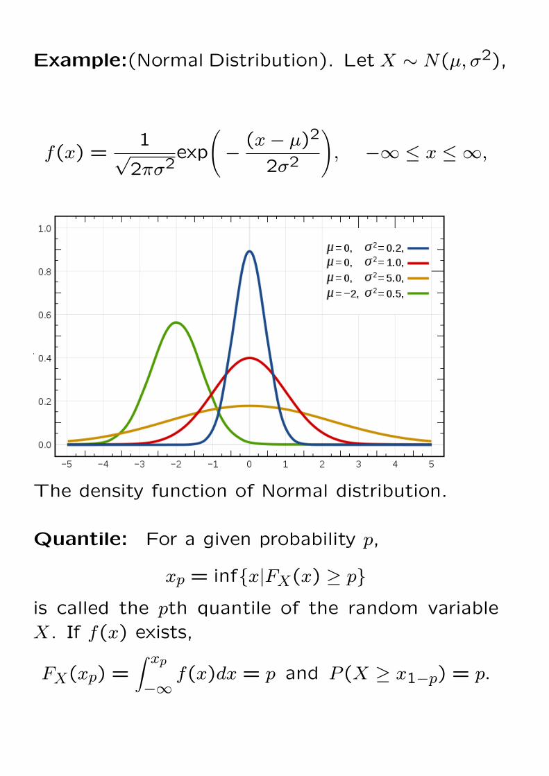
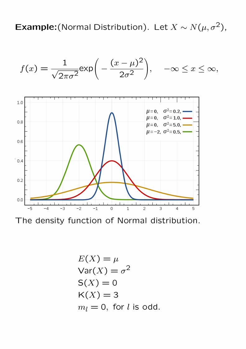
Example:(Normal Distribution). Let X ∼ N(µ, σ2),
f(x) =1√2πσ2
exp
(−
(x− µ)2
2σ2
), −∞ ≤ x ≤ ∞,
The density function of Normal distribution.
Quantile: For a given probability p,
xp = inf{x|FX(x) ≥ p}
is called the pth quantile of the random variableX. If f(x) exists,
FX(xp) =∫ xp
−∞f(x)dx = p and P (X ≥ x1−p) = p.
Moments of a random variable X:
Mean and variance:
µx = E(X) and σ2x = Var(X) = E(X − µx)2
Skewness (symmetry) and kurtosis (fat-tails)
S(x) = E(X − µx)3
σ3x, K(x) = E
(X − µx)4
σ4x.
K(x)− 3: Excess kurtosis.
The l−th moment and l−th central moment:
m′l = E(Xl) =
∫ ∞
−∞xlf(x)dx.
ml = E[(X − µx)l] =
∫ ∞
−∞(x− µx)
lf(x)dx,
Why are mean and variance of returns important?
They are concerned with long-term return and
risk, respectively.
Why is symmetry of interest in financial study?
Symmetry has important implications in holding
short or long financial positions and in risk man-
agement.
Why is kurtosis important?
Related to volatility forecasting, efficiency in esti-
mation and tests, etc.
High kurtosis implies heavy (or long) tails in dis-
tribution.
Example:(Normal Distribution). Let X ∼ N(µ, σ2),
f(x) =1√2πσ2
exp
(−
(x− µ)2
2σ2
), −∞ ≤ x ≤ ∞,
The density function of Normal distribution.
E(X) = µ
Var(X) = σ2
S(X) = 0
K(X) = 3
ml = 0, for l is odd.
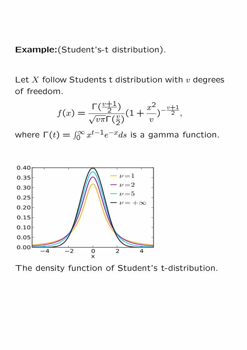
Example:(Student’s-t distribution).
Let X follow Students t distribution with v degrees
of freedom.
f(x) =Γ(v+1
2 )√vπΓ(v2)
(1 +x2
v)−
v+12 ,
where Γ(t) =∫∞0 xt−1e−xds is a gamma function.
The density function of Student’s t-distribution.
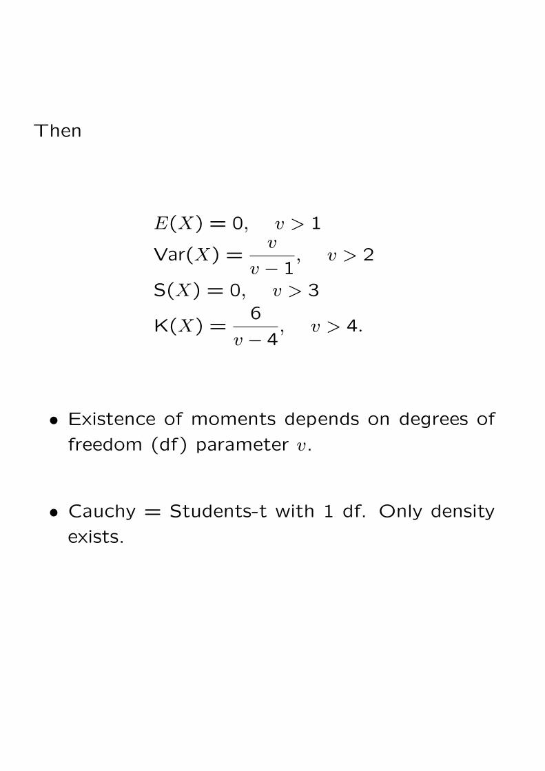
Then
E(X) = 0, v > 1
Var(X) =v
v − 1, v > 2
S(X) = 0, v > 3
K(X) =6
v − 4, v > 4.
• Existence of moments depends on degrees of
freedom (df) parameter v.
• Cauchy = Students-t with 1 df. Only density
exists.
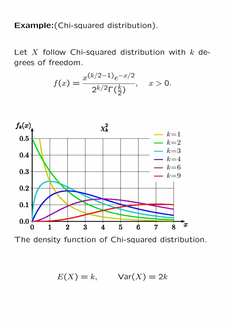
Example:(Chi-squared distribution).
Let X follow Chi-squared distribution with k de-
grees of freedom.
f(x) =x(k/2−1)e−x/2
2k/2Γ(k2), x > 0.
The density function of Chi-squared distribution.
E(X) = k, Var(X) = 2k
Joint Distribution: The following is a joint dis-tribution function of two variables:X and Y ,
FX,Y (x, y) = P (X ≤ x, Y ≤ y),
where x ∈ R, y ∈ R.
If the joint probability density function fx,y(x, y) ofX and Y exists, then
FX,Y (x, y) =∫ x
−∞
∫ y
−∞fx,y(w, z)dzdw.
Marginal Distribution: The marginal distributionof X is given by
FX(x) = FX,Y (x,∞).
Thus, the marginal distribution of X is obtainedby integrating out Y . A similar definition appliesto the marginal distribution of Y .
Conditional density function is
fx|y(x) ≡ fx,y(x, y)/fy(y) or
fx,y(x, y) = fx|y(x)× fy(y)
X and Y are independent random vectors if andonly if fx|y(x) = fx(x). In this case,
fx,y(x, y) = fx(x)× fy(y).
Estimation:
Data: {x1, · · · , xT}.
sample mean:
µx =1
T
T∑t=1
xt,
sample variance:
σ2x =1
T − 1
T∑t=1
(xt − µx)2,
sample skewness:
S(x) =1
(T − 1)σ3x
T∑t=1
(xt − µx)3,
sample kurtosis:
K(x) =1
(T − 1)σ4x
T∑t=1
(xt − µx)4.
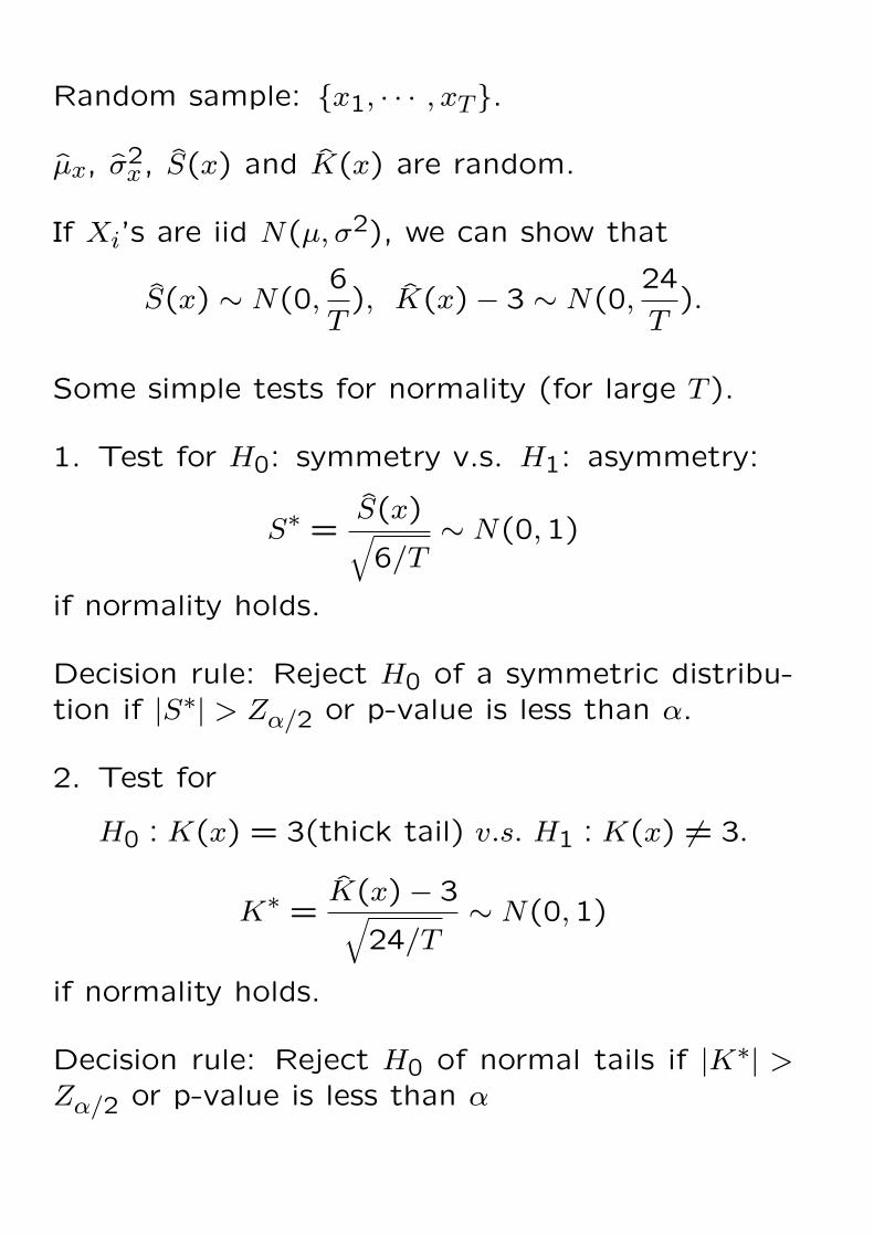
Random sample: {x1, · · · , xT}.
µx, σ2x, S(x) and K(x) are random.
If Xi’s are iid N(µ, σ2), we can show that
S(x) ∼ N(0,6
T), K(x)− 3 ∼ N(0,
24
T).
Some simple tests for normality (for large T ).
1. Test for H0: symmetry v.s. H1: asymmetry:
S∗ =S(x)√6/T
∼ N(0,1)
if normality holds.
Decision rule: Reject H0 of a symmetric distribu-tion if |S∗| > Zα/2 or p-value is less than α.
2. Test for
H0 : K(x) = 3(thick tail) v.s. H1 : K(x) = 3.
K∗ =K(x)− 3√
24/T∼ N(0,1)
if normality holds.
Decision rule: Reject H0 of normal tails if |K∗| >Zα/2 or p-value is less than α
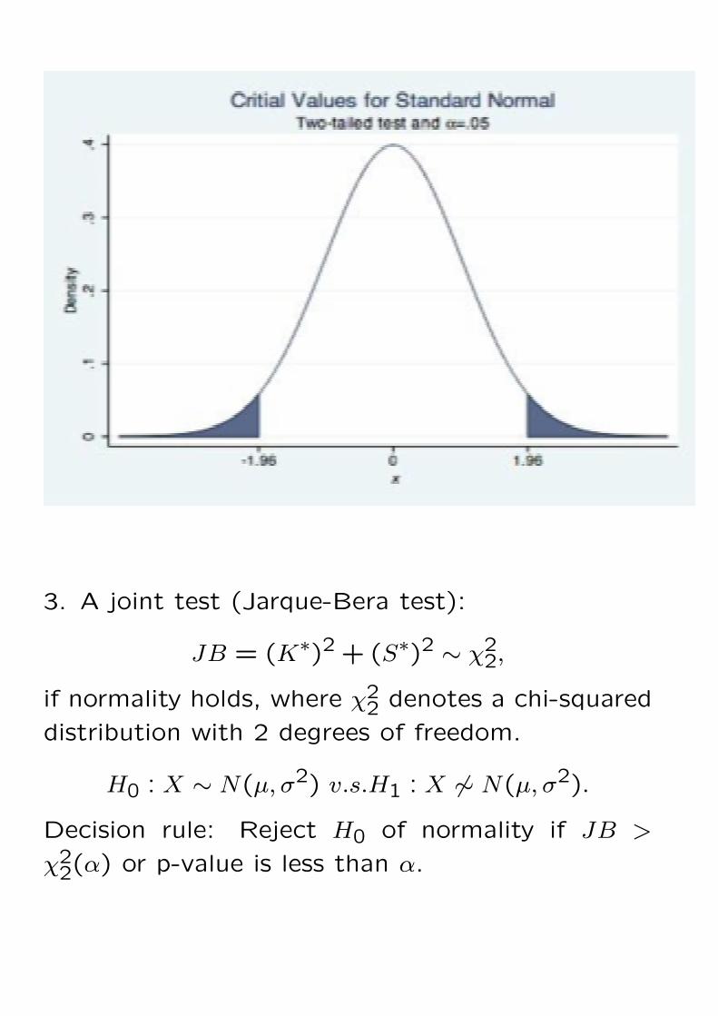
3. A joint test (Jarque-Bera test):
JB = (K∗)2 + (S∗)2 ∼ χ22,
if normality holds, where χ22 denotes a chi-squared
distribution with 2 degrees of freedom.
H0 : X ∼ N(µ, σ2) v.s.H1 : X ∼ N(µ, σ2).
Decision rule: Reject H0 of normality if JB >
χ22(α) or p-value is less than α.
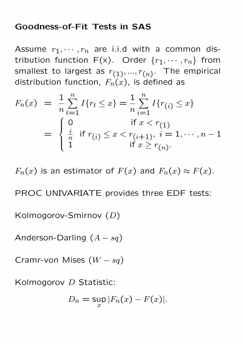
Goodness-of-Fit Tests in SAS
Assume r1, · · · , rn are i.i.d with a common dis-
tribution function F(x). Order {r1, · · · , rn} from
smallest to largest as r(1), ..., r(n). The empirical
distribution function, Fn(x), is defined as
Fn(x) =1
n
n∑t=1
I{rt ≤ x} =1
n
n∑i=1
I{r(i) ≤ x}
=
0 if x < r(1)in if r(i) ≤ x < r(i+1), i = 1, · · · , n− 11 if x ≥ r(n).
Fn(x) is an estimator of F (x) and Fn(x) ≈ F (x).
PROC UNIVARIATE provides three EDF tests:
Kolmogorov-Smirnov (D)
Anderson-Darling (A− sq)
Cramr-von Mises (W − sq)
Kolmogorov D Statistic:
Dn = supx
|Fn(x)− F (x)|.
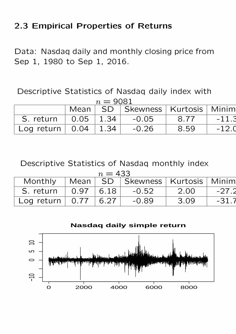
2.3 Empirical Properties of Returns
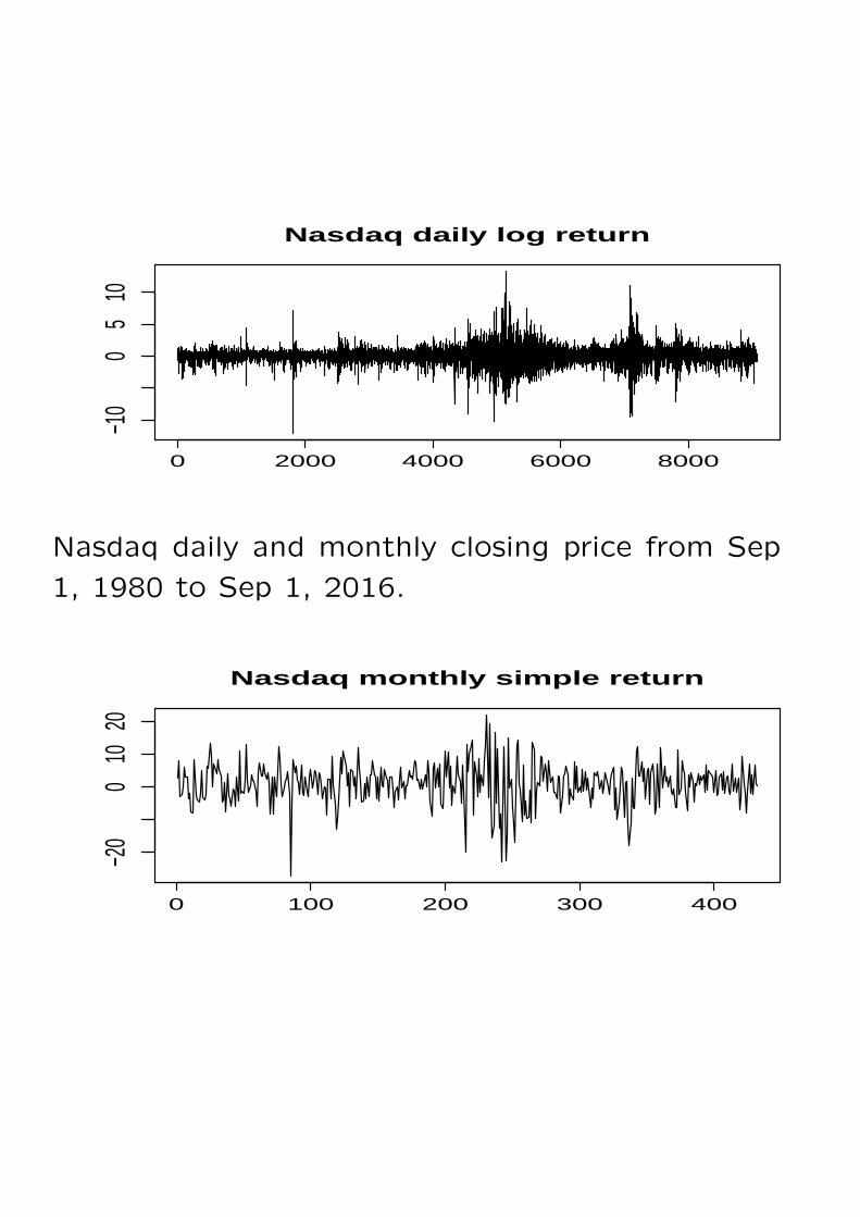
Data: Nasdaq daily and monthly closing price fromSep 1, 1980 to Sep 1, 2016.
Descriptive Statistics of Nasdaq daily index withn = 9081
Mean SD Skewness Kurtosis Minimum MaximumS. return 0.05 1.34 -0.05 8.77 -11.35 14.17Log return 0.04 1.34 -0.26 8.59 -12.04 13.25
Descriptive Statistics of Nasdaq monthly indexn = 433
Monthly Mean SD Skewness Kurtosis Minimum MaximumS. return 0.97 6.18 -0.52 2.00 -27.23 21.98Log return 0.77 6.27 -0.89 3.09 -31.79 19.87
0 2000 4000 6000 8000
−10
05
10
Nasdaq daily simple return
0 2000 4000 6000 8000
−10
05
10
Nasdaq daily log return
Nasdaq daily and monthly closing price from Sep
1, 1980 to Sep 1, 2016.
0 100 200 300 400
−20
010
20
Nasdaq monthly simple return
0 100 200 300 400
−30
−10
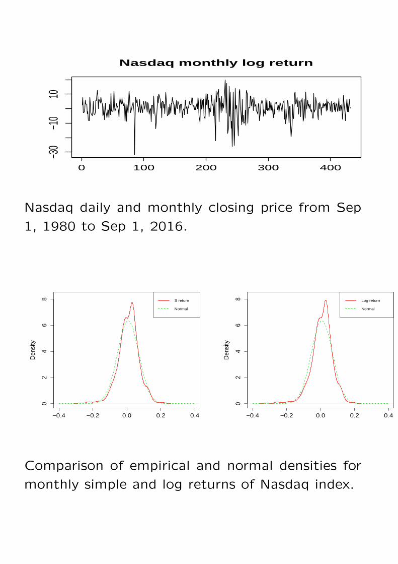
10Nasdaq monthly log return
Nasdaq daily and monthly closing price from Sep
1, 1980 to Sep 1, 2016.
−0.4 −0.2 0.0 0.2 0.4
02
46
8
Den
sity
S return
Normal
−0.4 −0.2 0.0 0.2 0.4
02
46
8
Den
sity
Log return
Normal
Comparison of empirical and normal densities for
monthly simple and log returns of Nasdaq index.
Related Documents