Computer Programming Modul Supardi, M.Si CHAPTER 1 INTRODUCTION TO MATLAB Matlab is short for Matrix Laboratory, which is a special-purpose computer program optimized to perform engineering and scientific calculations. It started life to perform matrix mathematics, but over the years it has grown into a flexible computing system capable of solving essentially any technical problem. Matlab implements a Matlab programming language and provides an extensive library of predifined functions that make technical programming tasks eisier and more eficient. 1 The Advantage of Matlab Matlab has many advantages compared with the conventional programming language like fortran, C or Pascal for technical problem solving. Among of them are the following: 1. Easy to Use. Matlab is intepreted language, so it is not needed compiling when we want to execute the program. Program may be easily writen and modified with the built-in integrated development inveronment and debuged with the Matlab debuger. 2. Platform Independence. Matlab is supported on many computer systems. At the time of tis writing, Matlab is supported on Windows 2000/ XP/Vista and many version of UNIX. Programs writen in any platform can run on all the other platforms and data files writen on any platform may be read on any 1

Welcome message from author
This document is posted to help you gain knowledge. Please leave a comment to let me know what you think about it! Share it to your friends and learn new things together.
Transcript

Computer Programming Modul Supardi, M.Si
CHAPTER 1
INTRODUCTION TO MATLABMatlab is short for Matrix Laboratory, which is a special-purpose computer
program optimized to perform engineering and scientific calculations. It started life
to perform matrix mathematics, but over the years it has grown into a flexible
computing system capable of solving essentially any technical problem. Matlab
implements a Matlab programming language and provides an extensive library of
predifined functions that make technical programming tasks eisier and more
eficient.
1 The Advantage of Matlab
Matlab has many advantages compared with the conventional programming
language like fortran, C or Pascal for technical problem solving. Among of them are
the following:
1. Easy to Use. Matlab is intepreted language, so it is not needed compiling
when we want to execute the program. Program may be easily writen and
modified with the built-in integrated development inveronment and
debuged with the Matlab debuger.
2. Platform Independence. Matlab is supported on many computer systems. At
the time of tis writing, Matlab is supported on Windows 2000/ XP/Vista and
many version of UNIX. Programs writen in any platform can run on all the
other platforms and data files writen on any platform may be read on any
1

Computer Programming Modul Supardi, M.Si
other proram.
3. Predefined Functions. Matlab comes complete with an extensive library of
predefined functions that provide tested and prepackaged solutions to many
technical problems. For example, suppose that you are writing a program
that calculate the stastitics associated with input data set. In most languages,
you need to write your own subroutines or functions to implement
calculations such as aritmatic mean, median, standard deviation and so forth.
These and hundreds of functions are built right into Matlab language,
making your job easier.
4. Device Independent Plotting. Unlike most other languages, Matlab has many
integral ploting and imaging commands. The plots and images can be
displayed on any graphical output device supported by computer on which
Matlab running. This capability makes Matlab an outstanding tool for
visualizing technical data.
5. Graphical User Interface (GUI). Matlab include tools that allow us to
interactively construct a Graphical User Interface (GUI) for his or her
program. With capability, the programmer can design a sophisticated data
analisys program that can be operated by relatively inexperienced users.
2 The Disadvantage of Matlab
There are two principal disadvantage of Matlab. First, because of Matlab is
intepreted language, therefor Matlab can run slowly compared with compiled
language such as pascal, c or fortran. Second, the disadvantage of Matlab is cost, full
2

Computer Programming Modul Supardi, M.Si
copy of Matlab may be 5 to 10 times more expensive than conventional compiler c,
pascal or fortran.
3 The Matlab Dekstop
When we start Matlab version 6.5, the special window called The Matlab
Dekstop will appear. The default configuration of Matlab Dekstop Matlab is shown
in Figure 1.1. It integrates many tools for managing files, variables and application
within Matlab environment.
The major tools within Matlab Dekstop are the following:
a) command window
b) command history window
c) launch pad
d) edit/debug window
e) figure window
f) workspace browser and array editor
g) help browser
h) current directory browser
Exercise1. Get help on Matlab function exp using: the “help exp” command typed on
the command window and get it with help browser.
3
Computer Programming Modul Supardi, M.Si
2.
4

Computer Programming Modul Supardi, M.Si
CHAPTER 2
MATLAB BASICS
1 Funncion and Constants
Matlab provides a large number of standard elementary mathematical
funsctions, including abs, sin, cos, sqrt, exp and so forth. Taking the square root of
negative number is not an error, because the appropriate complex number will be
produced automatically. Matlab also provide a large number of advanced
mathematical function, including bessel, gamma, beta, erf, and so forth. For a list of
standard elementary mathematical function, type
help elfun
and for a list of advanced mathematical functions, type
help specfun
Some functions, like sqrt, cos, sin,abs are built in. It means that they are has
been compiled, so we just apply them and computational details are not readily
accessible.
Matlab also provide some special constants that they may be useful to solve
any technical problem. Some constants are the following:
Tabel 2.3 Special Constants
No Constants Description
1 pi 3.14159265...
5

Computer Programming Modul Supardi, M.Si
2 i Imajinary unit, −1
3 j Same as i
4 eps Floating-point relative precision, 10-52
5 realmin Smallest floating-point number
6 realmax Largest floating-point number
7 inf Infinite number
8 NaN Not-a-Number
>> pi
ans =
3.1416
>> i
ans =
0 + 1.0000i
>> j
ans =
0 + 1.0000i
>> realmin
ans =
2.2251e-308
>> realmax
ans =
1.7977e+308
>> eps
ans =
6
Computer Programming Modul Supardi, M.Si
2.2204e-016
>> 1/0
Warning: Divide by zero.
ans =
Inf
>> 0/0
Warning: Divide by zero.
ans =
NaN
2 Using Meshgrid
Meshgrid is used to generate X and Y matrix for thrree dimensional plot. The
syntax of meshgrid are
[X,Y] = meshgrid(x,y)
[X,Y] = meshgrid(x)
[X,Y,Z] = meshgrid(x,y,z)
[X,Y]=meshgrid(x,y) transforms the domain specified by vector x and y into arrays X
and Y, which can be used to evaluate the function of two variables and three
dimensional mesh/surface plots. The rows of the output array X are copies of vector
x, and the column of the array Y are copies of the vector y.
Ex.
[X,Y] = meshgrid(1:3,10:14)
7
Computer Programming Modul Supardi, M.Si
X =
1 2 3
1 2 3
1 2 3
1 2 3
1 2 3
Y =
10 10 10
11 11 11
12 12 12
13 13 13
14 14 14
Contoh
Plot the function graphic of z=x2− y2 specified by domain 0x5 dan
0 y0
Solution
Firstly, we must specify the grids on the surface x-y using meshgrid function
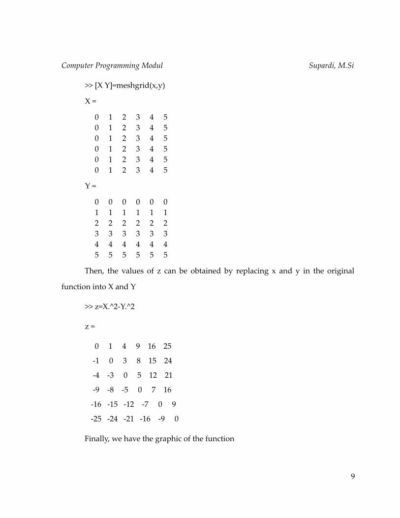
>> x=0:5;
>> y=0:5;
8
Computer Programming Modul Supardi, M.Si
>> [X Y]=meshgrid(x,y)
X =
0 1 2 3 4 5 0 1 2 3 4 5 0 1 2 3 4 5 0 1 2 3 4 5 0 1 2 3 4 5 0 1 2 3 4 5
Y =
0 0 0 0 0 0 1 1 1 1 1 1 2 2 2 2 2 2 3 3 3 3 3 3 4 4 4 4 4 4 5 5 5 5 5 5
Then, the values of z can be obtained by replacing x and y in the original
function into X and Y
>> z=X.^2-Y.^2
z =
0 1 4 9 16 25
-1 0 3 8 15 24
-4 -3 0 5 12 21
-9 -8 -5 0 7 16
-16 -15 -12 -7 0 9
-25 -24 -21 -16 -9 0
Finally, we have the graphic of the function
9

Computer Programming Modul Supardi, M.Si
>> mesh(X,Y,z)
3 Special Elementar Function Matlab
Matlab has a large number of special elementary function which may be
useful for numerical calculation. In this chapter, we will discuss some of them.
feval()
Function feval() is used to evaluate a function. For example, if we have a
function f x =x22 x1 and we evaluate the function at x=3
>> f=inline('x^2+2*x+1','x');
>> f(3)
10
Illustration 1:

Computer Programming Modul Supardi, M.Si
ans =
16
If we use the function provided by Matlab called humps. To evaluate the function,
we must create a handle function by using @ sign.
>> fhandle=@humps;
>> feval(fhandle,1)
ans =
16
11
Gambar 2.1 Fungsi humps

Computer Programming Modul Supardi, M.Si
Polyval
Function polyval is used to specify the value of the polynomial of the form
px =a0a1x1a2 x
2a3 x3a4 x
4...an−1xn−1an x
n
Matlab has a simply way to express the form of the polynomial by
p=[ an an−1 ... a3 a2 a1 a0 ]
Example
Given a polynomial px =x 43x 24x5 . It will be evaluated at
x=2, −3 and 4.
Solution
● First, we type the polynomial by simply way p=[1 0 3 4 5].
● Second, we type the point we are going to evaluate x=[2,-3,4]
● Third, Evaluate the polynomial at point x by command polyval(p,x)
If we write in the command window
>> p=[1 0 3 4 5];
>> x=[2,-3,4];
>> polyval(p,x)
ans =
41 101 325
12
Computer Programming Modul Supardi, M.Si
Polyfit
Fungsi polyder
Fungsi poly
Fungsi conv
Fungsi deconv
13

Computer Programming Modul Supardi, M.Si
CHAPTER 3
VECTOR AND MATRICES
Vector is one-dimensional array of numbers. Vector can be a coulomn or row.
Matlab can create a coulomn vector by enclosing a set of numbers sparated by
semicolon. For example, to create a coulomn vector with three elements we write:
>> a=[1;2;3]
a =
1
2
3
To create a row vector, we enclose a set of numbers in square brackets, but this time
we use coma or blank space to delimite the elements.
>> a=[4,5,6]
a =
4 5 6
>> a=[4 5 6]
a =
4 5 6
14

Computer Programming Modul Supardi, M.Si
A column vector can be turned into a row vector by three ways. The first, we
can turn using the transpose operation.
>> v=[3,2,1];
>> v'
ans =
3
2
1
Secondly, we can create a column vector by enclosing a set of numbers with
semicolon notation to delimite the numbers.
>> w=[3;2;1]
w =
3
2
1
It is also possible to add or subtract two vectorsto produce a new vector. In
order to perform this operation, the two vectors must both be the same type and the
same length. So, we can add two column vectors together to produce a new column
vector or we can add two row vector to produce a new row vector. Lets add two
column vectors together:
15
Computer Programming Modul Supardi, M.Si
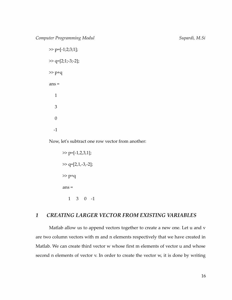
>> p=[-1;2;3;1];
>> q=[2;1;-3;-2];
>> p+q
ans =
1
3
0
-1
Now, let's subtract one row vector from another:
>> p=[-1,2,3,1];
>> q=[2,1,-3,-2];
>> p+q
ans =
1 3 0 -1
1 CREATING LARGER VECTOR FROM EXISTING VARIABLES
Matlab allow us to append vectors together to create a new one. Let u and v
are two column vectors with m and n elements respectively that we have created in
Matlab. We can create third vector w whose first m elements of vector u and whose
second n elements of vector v. In order to create the vector w, it is done by writing
16
Computer Programming Modul Supardi, M.Si
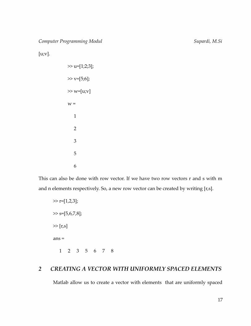
[u;v].
>> u=[1;2;3];
>> v=[5;6];
>> w=[u;v]
w =
1
2
3
5
6
This can also be done with row vector. If we have two row vectors r and s with m
and n elements respectively. So, a new row vector can be created by writing [r,s].
>> r=[1,2,3];
>> s=[5,6,7,8];
>> [r,s]
ans =
1 2 3 5 6 7 8
2 CREATING A VECTOR WITH UNIFORMLY SPACED ELEMENTS
Matlab allow us to create a vector with elements that are uniformly spaced
17

Computer Programming Modul Supardi, M.Si
by increment q. To create a vector x that have unformly spaced elements with first
element a, final element b and stepsize q is
x= [ a : q : b];
We can create a list of even number from 0 to 10 with uniformly spaced elements:
>> x=[0:2:10]
x =
0 2 4 6 8 10
Again, let's we create a list of small number starts from 0 to 1 with uniformly space
0.1;
>> x=0:0.1:1
x =
Columns 1 through 7
0 0.1000 0.2000 0.3000 0.4000 0.5000 0.6000
Columns 8 through 11
0.7000 0.8000 0.9000 1.0000
The set of x values can be used to create a list of points representing the values of
some given function. For example, suppose that whave y=e x , then we have
>> y=exp(x)
y =
Columns 1 through 7
18
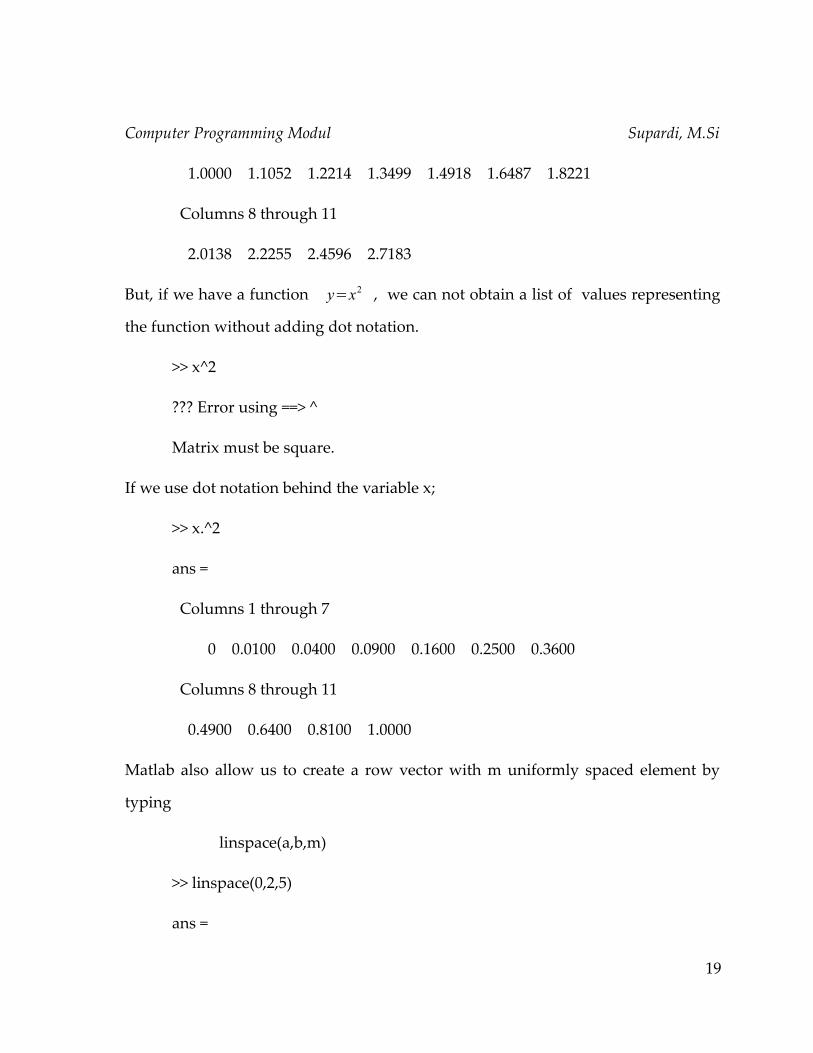
Computer Programming Modul Supardi, M.Si
1.0000 1.1052 1.2214 1.3499 1.4918 1.6487 1.8221
Columns 8 through 11
2.0138 2.2255 2.4596 2.7183
But, if we have a function y=x2 , we can not obtain a list of values representing
the function without adding dot notation.
>> x^2
??? Error using ==> ^
Matrix must be square.
If we use dot notation behind the variable x;
>> x.^2
ans =
Columns 1 through 7
0 0.0100 0.0400 0.0900 0.1600 0.2500 0.3600
Columns 8 through 11
0.4900 0.6400 0.8100 1.0000
Matlab also allow us to create a row vector with m uniformly spaced element by
typing
linspace(a,b,m)
>> linspace(0,2,5)
ans =
19

Computer Programming Modul Supardi, M.Si
0 0.5000 1.0000 1.5000 2.0000
Matlab also allow us to create a a row vector with n logaritmically spaced
elements by typing
logspace(a,b,n)
>> logspace(1,3,5)
ans =
1.0e+003 *
0.0100 0.0316 0.1000 0.3162 1.0000
3 Characterizing Vector
The length command returns a number of a vector elements, for example:
>> a=[0:5];
>> length(a)
ans =
6
We can find the largest and smallest of a vector by max and min command,
ffor example:
>> a=[0:5];
>> max(a)
ans =
20
Computer Programming Modul Supardi, M.Si
5
>> min(a)
ans =
0
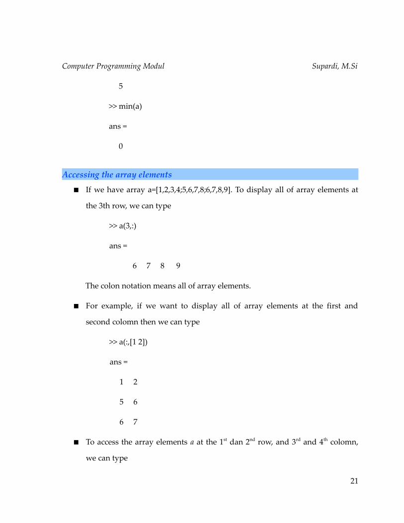
Accessing the array elements
If we have array a=[1,2,3,4;5,6,7,8;6,7,8,9]. To display all of array elements at
the 3th row, we can type
>> a(3,:)
ans =
6 7 8 9
The colon notation means all of array elements.
For example, if we want to display all of array elements at the first and
second colomn then we can type
>> a(:,[1 2])
ans =
1 2
5 6
6 7
To access the array elements a at the 1st dan 2nd row, and 3rd and 4th colomn,
we can type
21
Computer Programming Modul Supardi, M.Si
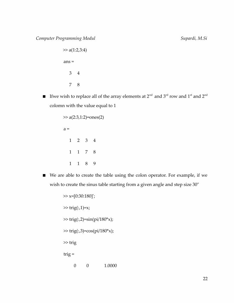
>> a(1:2,3:4)
ans =
3 4
7 8
Ifwe wish to replace all of the array elements at 2nd and 3rd row and 1st and 2nd
colomn with the value equal to 1
>> a(2:3,1:2)=ones(2)
a =
1 2 3 4
1 1 7 8
1 1 8 9
We are able to create the table using the colon operator. For example, if we
wish to create the sinus table starting from a given angle and step size 30o
>> x=[0:30:180]';
>> trig(:,1)=x;
>> trig(:,2)=sin(pi/180*x);
>> trig(:,3)=cos(pi/180*x);
>> trig
trig =
0 0 1.0000
22

Computer Programming Modul Supardi, M.Si
30.0000 0.5000 0.8660
60.0000 0.8660 0.5000
90.0000 1.0000 0.0000
120.0000 0.8660 -0.5000
150.0000 0.5000 -0.8660
180.0000 0.0000 -1.0000
The Colon operator can be used to perform the operation at Gauss
elimination. For example
>> a=[-1,1,2,2;8,2,5,3;10,-4,5,3;7,4,1,-5];
>> a(2,:)=a(2,:)-a(2,1)/a(1,1)*a(1,:)
a =
-1.00 1.00 2.00 2.00
0 10.00 21.00 19.00
10.00 -4.00 5.00 3.00
7.00 4.00 1.00 -5.00
>> a(3,:)=a(3,:)-a(3,1)/a(1,1)*a(1,:)
a =
-1.00 1.00 2.00 2.00
0 10.00 21.00 19.00
23

Computer Programming Modul Supardi, M.Si
0 6.00 25.00 23.00
7.00 4.00 1.00 -5.00
>> a(4,:)=a(4,:)-a(4,1)/a(1,1)*a(1,:)
a =
-1.00 1.00 2.00 2.00
0 10.00 21.00 19.00
0 6.00 25.00 23.00
0 11.00 15.00 9.00
>> a(3,:)=a(3,:)-a(3,2)/a(2,2)*a(2,:)
a =
-1.00 1.00 2.00 2.00
0 10.00 21.00 19.00
0 0 12.40 11.60
0 11.00 15.00 9.00
>> a(4,:)=a(4,:)-a(4,2)/a(2,2)*a(2,:)
a =
-1.00 1.00 2.00 2.00
0 10.00 21.00 19.00
0 0 12.40 11.60
24

Computer Programming Modul Supardi, M.Si
0 0 -8.10 -11.90
>> a(4,:)=a(4,:)-a(4,3)/a(3,3)*a(3,:)
a =
-1.00 1.00 2.00 2.00
0 10.00 21.00 19.00
0 0 12.40 11.60
0 0 0 -4.32
The keyword end states the final element of the array elements. For example,
if we have a vector
>> a=[1:6];
>> a(end)
ans =
6
>> sum(a(2:end))
ans =
20
The colon operator can play as a single subscript. For a spcial case, the colon
operator can be used to replace all of the array elements
>> a=[1:4;5:8]
a =
25

Computer Programming Modul Supardi, M.Si
1 2 3 4
5 6 7 8
>> a(:)=-1
a =
-1 -1 -1 -1
-1 -1 -1 -1
Replication of row and column
Sometimes, we need to generate the array elements at a given row and
column to any other row and column. For this purpose, we need Matlab command
repmat to replicate the row/column elements.
>> a=[1;2;3];
>> b=repmat(a,[1 3])
b =
1 1 1
2 2 2
3 3 3
The command repmat(a,[1 3]) means that “replicate vector a into one row and three
columns.
>> c=repmat(a,[2 1])
c =
26

Computer Programming Modul Supardi, M.Si
1
2
3
1
2
3
The command repmat(a,[2 1]) means that “replicate vector a into two rows
and 1 column.
The alternative command repmat (a,[1 3]) is repmat(a,1,3) and repmat (a,[2 1])
is repmat(a,2,1).
Deleting rows and columns
We can use the colon operator and the blank array to delete the array
elements.
>> b=[1,2,3;3,4,5;6,7,8]
b =
1 2 3
3 4 5
6 7 8
>> b(:,2)=[]
b =
27
Computer Programming Modul Supardi, M.Si
1 3
3 5
6 8
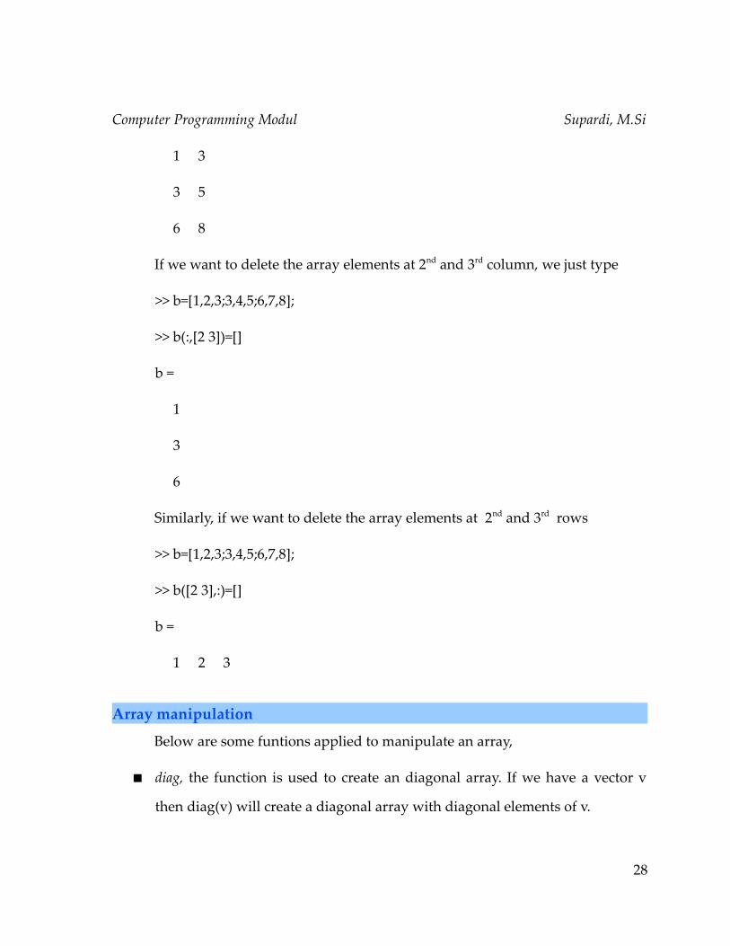
If we want to delete the array elements at 2nd and 3rd column, we just type
>> b=[1,2,3;3,4,5;6,7,8];
>> b(:,[2 3])=[]
b =
1
3
6
Similarly, if we want to delete the array elements at 2nd and 3rd rows
>> b=[1,2,3;3,4,5;6,7,8];
>> b([2 3],:)=[]
b =
1 2 3
Array manipulation
Below are some funtions applied to manipulate an array,
diag, the function is used to create an diagonal array. If we have a vector v
then diag(v) will create a diagonal array with diagonal elements of v.
28

Computer Programming Modul Supardi, M.Si
>> v=[1:4];
>> diag(v)
ans =
1 0 0 0
0 2 0 0
0 0 3 0
0 0 0 4
To move right or move down the diagonal elements, we just type diag(v,b)
>> diag(v,2)
ans =
0 0 1 0 0 0
0 0 0 2 0 0
0 0 0 0 3 0
0 0 0 0 0 4
0 0 0 0 0 0
0 0 0 0 0 0
>> diag(v,-2)
ans =
0 0 0 0 0 0
0 0 0 0 0 0
29
Computer Programming Modul Supardi, M.Si
1 0 0 0 0 0
0 2 0 0 0 0
0 0 3 0 0 0
0 0 0 4 0 0
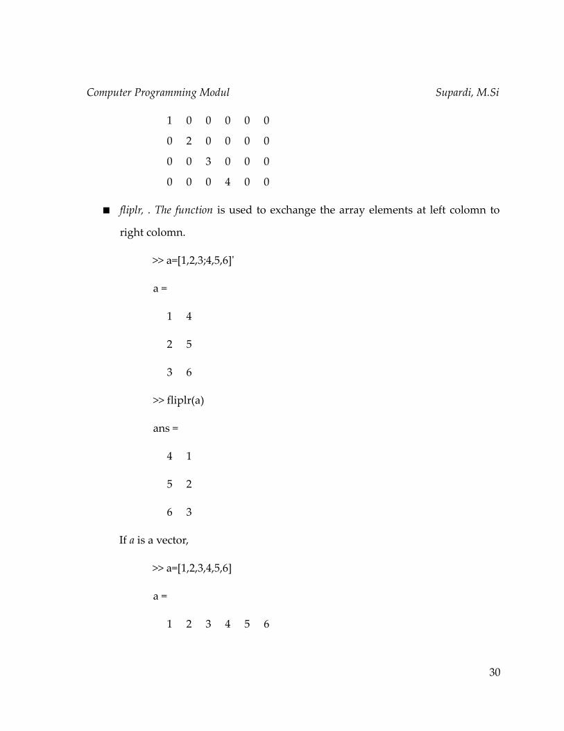
fliplr, . The function is used to exchange the array elements at left colomn to
right colomn.
>> a=[1,2,3;4,5,6]'
a =
1 4
2 5
3 6
>> fliplr(a)
ans =
4 1
5 2
6 3
If a is a vector,
>> a=[1,2,3,4,5,6]
a =
1 2 3 4 5 6
30

Computer Programming Modul Supardi, M.Si
>> fliplr(a)
ans =
6 5 4 3 2 1
flipud, this function is used to exchange the array elements at the upper row
to lower row.
>> a=[1,2,3;4,5,6]
a =
1 2 3
4 5 6
>> flipud(a)
ans =
4 5 6
1 2 3
rot90, this function is used to rotate matrix A with 90o counter clockwise.
>> a=[1,2,3;4,5,6]
a =
1 2 3
4 5 6
>> rot90(a)
31
Computer Programming Modul Supardi, M.Si
ans =
3 6
2 5
1 4
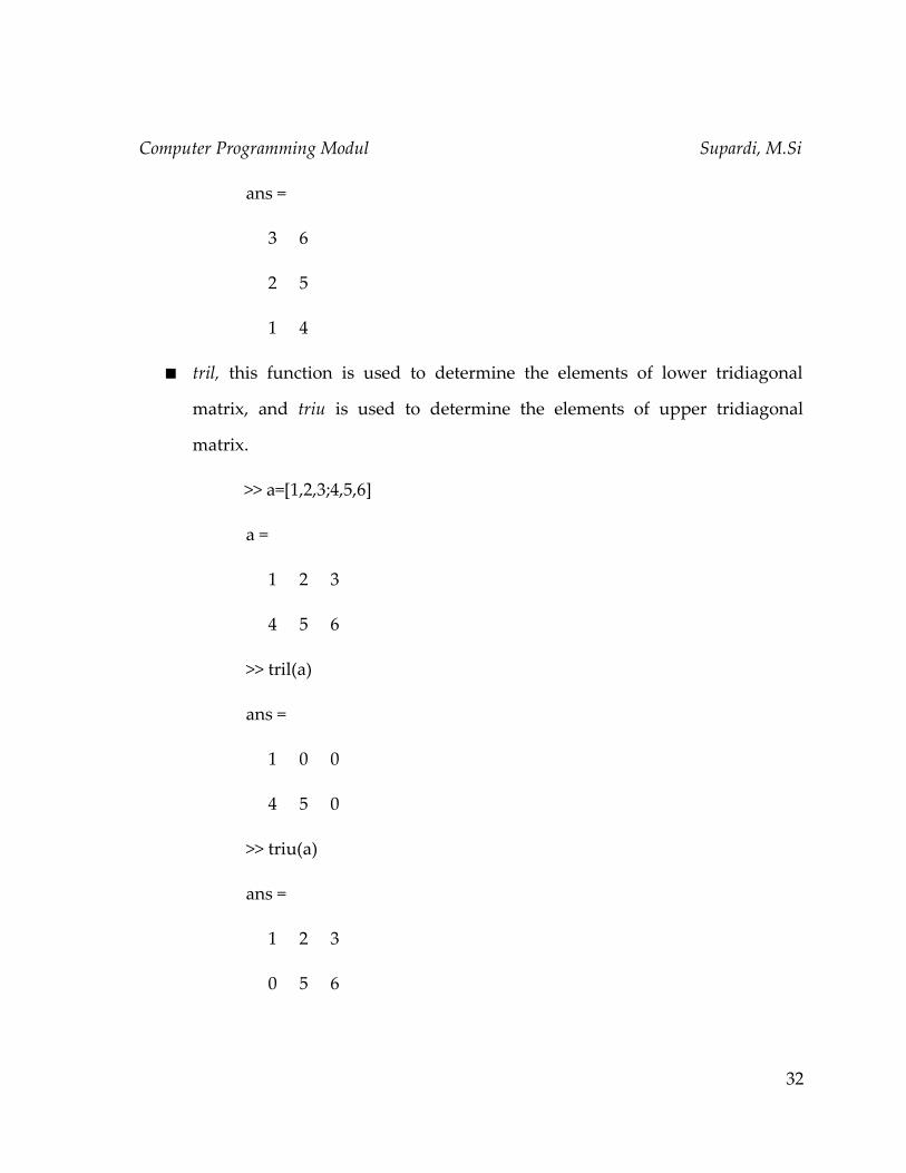
tril, this function is used to determine the elements of lower tridiagonal
matrix, and triu is used to determine the elements of upper tridiagonal
matrix.
>> a=[1,2,3;4,5,6]
a =
1 2 3
4 5 6
>> tril(a)
ans =
1 0 0
4 5 0
>> triu(a)
ans =
1 2 3
0 5 6
32

Computer Programming Modul Supardi, M.Si
Another Functions in Matlab
Masih ada banyak fungsi yang dapat digunakan untuk manipulasi matriks.
Beberapa diantaranya
det,fungsi ini digunakan untuk menentukan determinan matriks. Ingat,
bahwa matriks yang memimiliki determinan hanyalah matriks bujur sangkar.
>> a=[1,2,3;4,3,-2;-1,5,2];
>> det(a)
ans =
73
eig, ini digunakan untuk menentukan nilai eigen.
>> a=[1,2,3;4,3,-2;-1,5,2];
>> eig(a)
ans =
5.5031
0.2485 + 3.6337i
0.2485 – 3.6337i
inv, fungsi ini digunakan untuk melakukan invers matriks seperti telah
dijelaskan di atas.
lu, adalah fungsi untuk melakukan dekomposisi matriks menjadi matriks
segitiga bawah dan matriks segitiga atas.
33

Computer Programming Modul Supardi, M.Si
>> a=[1,2,3;4,3,-2;-1,5,2];
>> [L,U]=lu(a)
L =
0.25 0.22 1.00
1.00 0 0
-0.25 1.00 0
U =
4.00 3.00 -2.00
0 5.75 1.50
0 0 3.17
34
Computer Programming Modul Supardi, M.Si
CHAPTER 4
INTRODUCTION TO GRAPHICS
Basic 2-D graphs
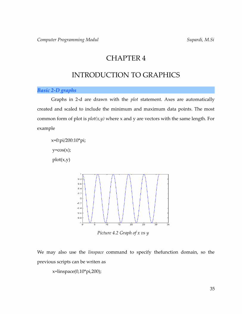
Graphs in 2-d are drawn with the plot statement. Axes are automatically
created and scaled to include the minimum and maximum data points. The most
common form of plot is plot(x,y) where x and y are vectors with the same length. For
example
x=0:pi/200:10*pi;
y=cos(x);
plot(x,y)
We may also use the linspace command to specify thefunction domain, so the
previous scripts can be writen as
x=linspace(0,10*pi,200);
35
Picture 4.2 Graph of x vs y

Computer Programming Modul Supardi, M.Si
y=cos(x);
plot(x,y)
Multiple plot on the same axes
There are at least two ways of drawing multiple plots on the same axes. The
ways are followings:
1. The simplest way is to use hold to keep the current plot on the axes. All
subsequents plots are added to the axes until hold is released. For example,
x=linspace(0,2*pi,200);
y1=cos(x);
plot(x,y1);
hold;
y2=cos(x-0.5);
plot(x,y2);
y3=cos(x-1.0);
plot(x,y3)
36
Picture 4.2 Creating multiple graphs on the same axes with hold
Computer Programming Modul Supardi, M.Si
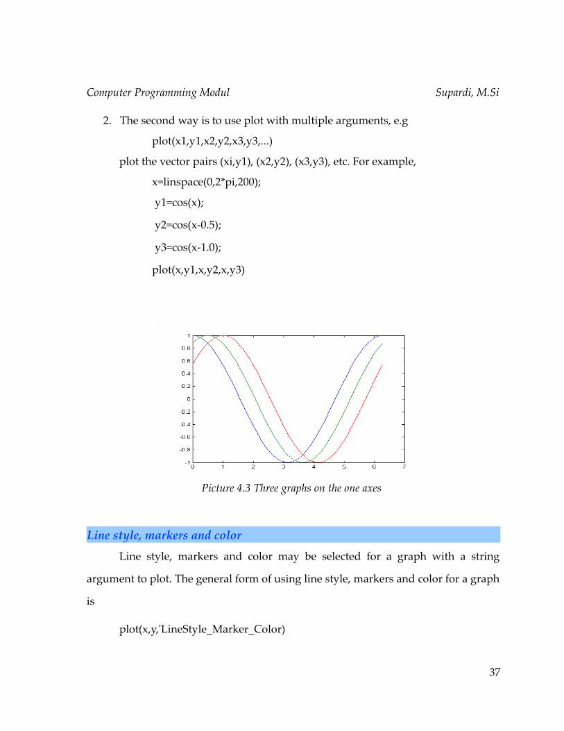
2. The second way is to use plot with multiple arguments, e.g
plot(x1,y1,x2,y2,x3,y3,...)
plot the vector pairs (xi,y1), (x2,y2), (x3,y3), etc. For example,
x=linspace(0,2*pi,200);
y1=cos(x);
y2=cos(x-0.5);
y3=cos(x-1.0);
plot(x,y1,x,y2,x,y3)
Line style, markers and color
Line style, markers and color may be selected for a graph with a string
argument to plot. The general form of using line style, markers and color for a graph
is
plot(x,y,'LineStyle_Marker_Color)
37
Picture 4.3 Three graphs on the one axes

Computer Programming Modul Supardi, M.Si
For example
x=linspace(0,2*pi,200);
y1=cos(x);
y2=cos(x-0.5);
y3=cos(x-1.0);
plot(x,y1,'-',x,y2,'o',x,y3,':')
grid
Notice that picture 4.4 is displayed with grids. The grids can be accompanied
on the graph with grid command.
x=linspace(0,2*pi,200);
y=cos(x);
plot(x,y,'-squarer')
38
Picture 4.4. Displaying three graphs with different line style
Computer Programming Modul Supardi, M.Si
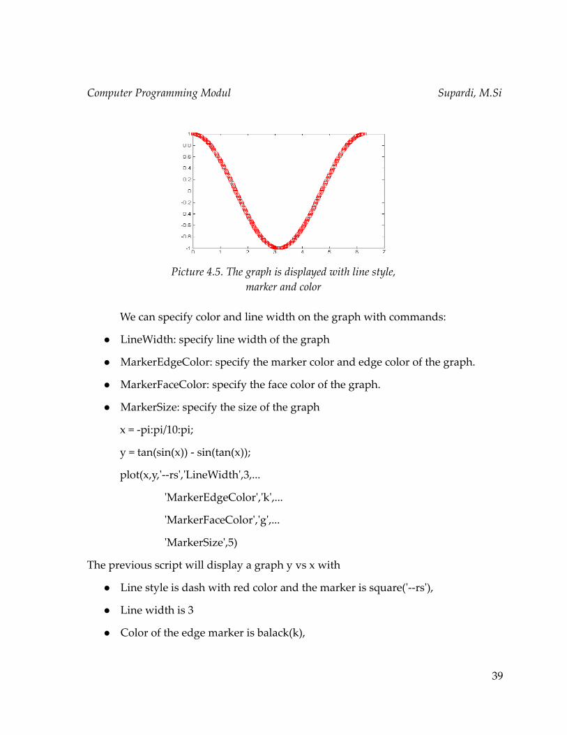
We can specify color and line width on the graph with commands:
LineWidth: specify line width of the graph
MarkerEdgeColor: specify the marker color and edge color of the graph.
MarkerFaceColor: specify the face color of the graph.
MarkerSize: specify the size of the graph
x = -pi:pi/10:pi;
y = tan(sin(x)) - sin(tan(x));
plot(x,y,'--rs','LineWidth',3,...
'MarkerEdgeColor','k',...
'MarkerFaceColor','g',...
'MarkerSize',5)
The previous script will display a graph y vs x with
Line style is dash with red color and the marker is square('--rs'),
Line width is 3
Color of the edge marker is balack(k),
39
Picture 4.5. The graph is displayed with line style, marker and color
Computer Programming Modul Supardi, M.Si
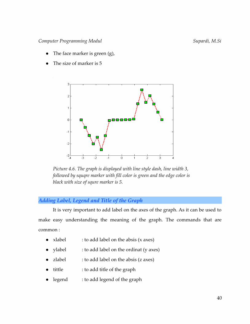
The face marker is green (g),
The size of marker is 5
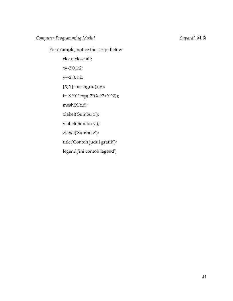
Adding Label, Legend and Title of the Graph
It is very important to add label on the axes of the graph. As it can be used to
make easy understanding the meaning of the graph. The commands that are
common :
xlabel : to add label on the absis (x axes)
ylabel : to add label on the ordinat (y axes)
zlabel : to add label on the absis (z axes)
tittle : to add title of the graph
legend : to add legend of the graph
40
Picture 4.6. The graph is displayed with line style dash, line width 3, followed by squqre marker with fill color is green and the edge color is black with size of squre marker is 5.
Computer Programming Modul Supardi, M.Si
For example, notice the script below
clear; close all;
x=-2:0.1:2;
y=-2:0.1:2;
[X,Y]=meshgrid(x,y);
f=-X.*Y.*exp(-2*(X.^2+Y.^2));
mesh(X,Y,f);
xlabel('Sumbu x');
ylabel('Sumbu y');
zlabel('Sumbu z');
title('Contoh judul grafik');
legend('ini contoh legend')
41

Computer Programming Modul Supardi, M.Si
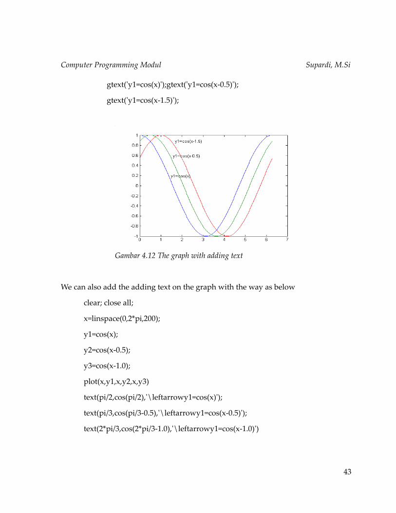
Adding Text on the Graph
Sometime, we need to add any text to make clearly if there are more than one
graph on the one axes. To add some texts one the graph, we can use gtext(). For
example
clear; close all;
x=linspace(0,2*pi,200);
y1=cos(x);
y2=cos(x-0.5);
y3=cos(x-1.0);
plot(x,y1,x,y2,x,y3);
42
Picture 4.12
Computer Programming Modul Supardi, M.Si
gtext('y1=cos(x)');gtext('y1=cos(x-0.5)');
gtext('y1=cos(x-1.5)');
We can also add the adding text on the graph with the way as below
clear; close all;
x=linspace(0,2*pi,200);
y1=cos(x);
y2=cos(x-0.5);
y3=cos(x-1.0);
plot(x,y1,x,y2,x,y3)
text(pi/2,cos(pi/2),'\leftarrowy1=cos(x)');
text(pi/3,cos(pi/3-0.5),'\leftarrowy1=cos(x-0.5)');
text(2*pi/3,cos(2*pi/3-1.0),'\leftarrowy1=cos(x-1.0)')
43
Gambar 4.12 The graph with adding text

Computer Programming Modul Supardi, M.Si
CHAPTER 6
FLOW CONTROL
There are eight flow control statements in MATLAB:
1. if, together with else and elseif, executes a group of statements based on some
logical condition.
2. switch, together with case and otherwise, executes different groups of
statements depending on the value of some logical condition.
3. while executes a group of statements an indefinite number of times, based on
some logical condition.
4. for executes a group of statements a fixed number of times.
5. continue passes control to the next iteration of a for or while loop, skipping
any remaining statements in the body of the loop.
6. break terminates execution of a for or while loop.
7. try...catch changes flow control if an error is detected during execution.
8. return causes execution to return to the invoking function. All flow constructs
use end to indicate the end of the flow control block.
if, else, and elseif evaluates a logical expression and executes a group of
statements based on the value of the expression. In its simplest form, its syntax is
44

Computer Programming Modul Supardi, M.Si
if (logical_expression)
statements
end
If the logical expression is true (1), MATLAB executes all the statements between the
if and end lines. It resumes execution at the line following the end statement. If the
condition is false (0), MATLAB skips all the statements between the if and end lines,
and resumes execution at the line following the end statement. For example,
if mod(a,2) == 0
disp('a is even')
b = a/2;
end
The if statement can be desribed in the diagram as picture 3 below
45
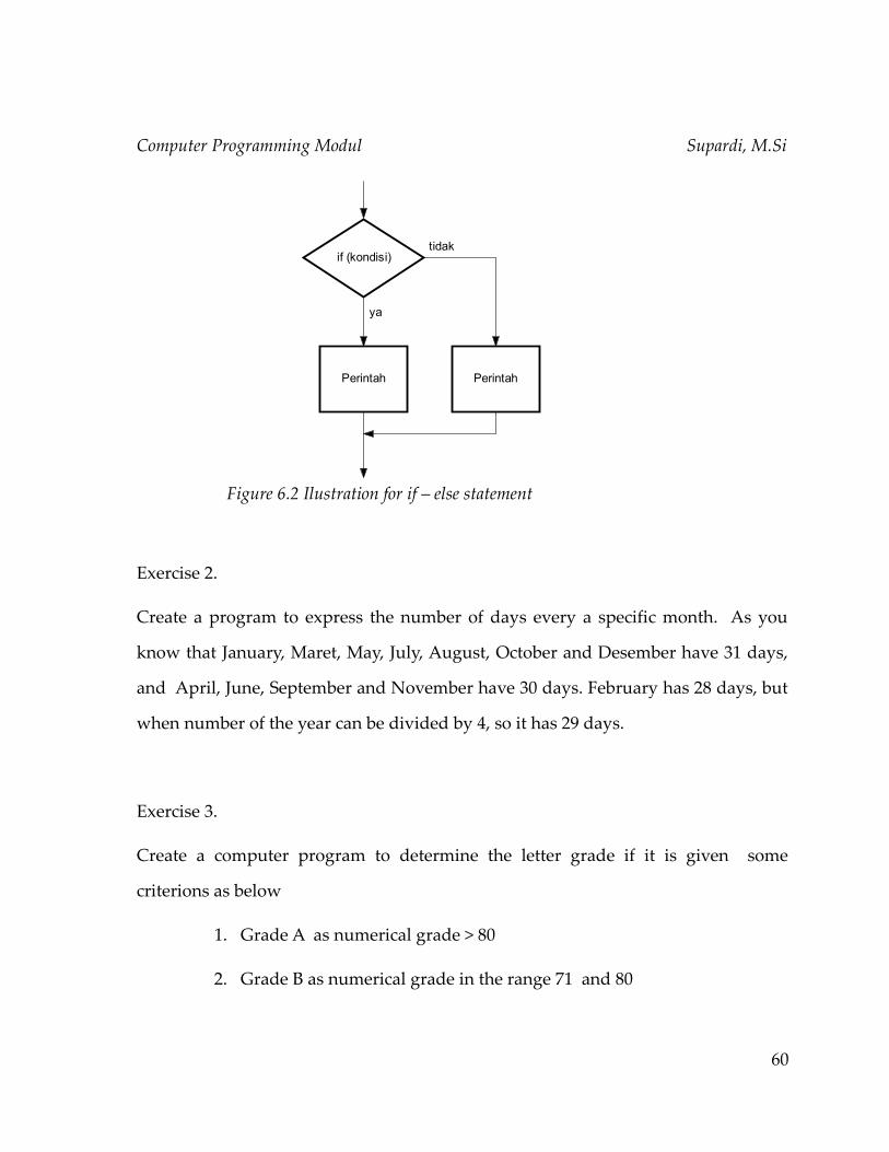
Gambar 6.1 Diagram alir percabangan if
if (kondisi)
Perintah
ya
tidak

Computer Programming Modul Supardi, M.Si
Generally, the condition is logical expression, that is, the expression consisting of
relational operator that is true (1) or false (0). The followings are some relational operators:
Relational Operator
Meaning
< Less than<= Less than or equal > Greater than>= Greater than or equal== Equal to~= Not equal
The followings are some examples of logical expression using relational operator
and its meaning
b^2-4*a*c<0 b2−4a c0
b^2>4*a*c b24 ac
b^2-4*a*c==0 b2−4a c =0
b~=4 b≠4
There are also some logical operators as below
Logical Operator
Symbol Meaning
And & AndOr | OrNot ~ notXor Eksklusiv Or
The following is a table to describe the value of the expression with logical operator.
46

Computer Programming Modul Supardi, M.Si
a b a&b a|b ~a ~b a xor b
TRUE TRUE TRUE TRUE FALSE FALSE FALSE
TRUE FALSE FALSE TRUE FALSE TRUE TRUE
FALSE TRUE FALSE TRUE TRUE FALSE TRUE
FALSE FALSE FALSE FALSE TRUE TRUE FALSE
1 else and elseif statements
The else statement has no logical condition. The statements associated with it
execute if the preceding if (and possibly elseif condition) is false (0). The elseif
statement has a logical condition that it evaluates if the preceding if (and possibly
elseif condition) is false (0). The statements associated with it execute if its logical
condition is true (1). You can have multiple elseifs within an if block. if n < 0
% If n negative, display error message.
disp('Input must be positive');
elseif rem(n,2) == 0 % If n positive and even, divide by 2.
A = n/2;
else
A = (n+1)/2; % If n positive and odd, increment and divide.
end
47
Computer Programming Modul Supardi, M.Si
if Statements and Empty ArraysAn if condition that reduces to an empty array
represents a false condition. That is, if A
S1
else
S0
end
will execute statement S0 when A is an empty array.
48

Computer Programming Modul Supardi, M.Si
49

Computer Programming Modul Supardi, M.Si
50
Computer Programming Modul Supardi, M.Si
51
Computer Programming Modul Supardi, M.Si
52
Computer Programming Modul Supardi, M.Si
53
Computer Programming Modul Supardi, M.Si
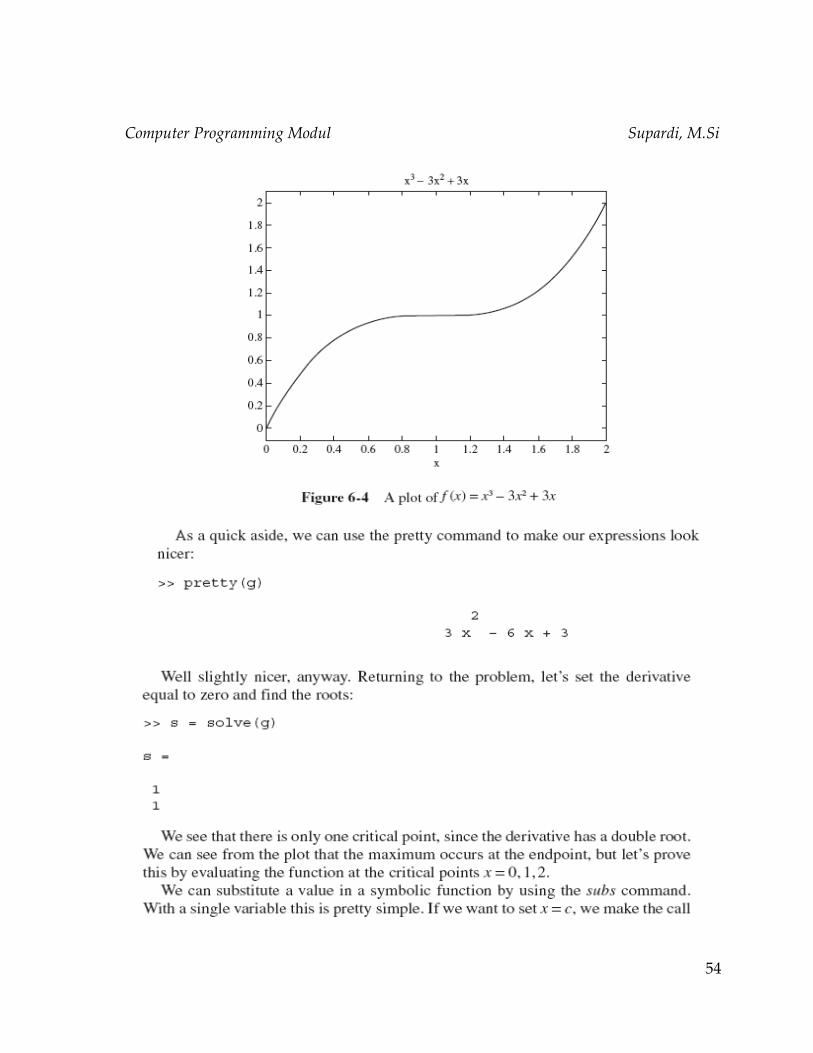
54
Computer Programming Modul Supardi, M.Si
55

Computer Programming Modul Supardi, M.Si
CHAPTER 6
FLOW CONTROL
1 Introduction
There are eight flow control statements in MATLAB:
1. if, together with else and elseif, executes a group of statements based on some
logical condition.
2. switch, together with case and otherwise, executes different groups of
statements depending on the value of some logical condition.
3. while executes a group of statements an indefinite number of times, based on
some logical condition.
4. for executes a group of statements a fixed number of times.
5. continue passes control to the next iteration of a for or while loop, skipping
any remaining statements in the body of the loop.
6. break terminates execution of a for or while loop.
7. try...catch changes flow control if an error is detected during execution.
8. return causes execution to return to the invoking function. All flow constructs
56

Computer Programming Modul Supardi, M.Si
use end to indicate the end of the flow control block.
2 The if Statement
The flow control, if, else, and elseif evaluates a logical expression and
executes a group of statements based on the value of the expression. In its simplest
form, its syntax is
if (logical_expression)
statements
end
If the logical expression is true (1), MATLAB executes all the statements between
the if and end lines. It resumes execution at the line following the end statement. If
the condition is false (0), MATLAB skips all the statements between the if and end
lines, and resumes execution at the line following the end statement. For example,
a=3;
if (a>2)
disp('TRUE')
end
The if statement can be desribed in the diagram as picture 3 below
57

Computer Programming Modul Supardi, M.Si
Generally, the condition is logical expression, that is, the expression consisting of
relational operator that is true (1) or false (0). The followings are some relational operators:
Relational Operator
Meaning
< Less than<= Less than or equal > Greater than>= Greater than or equal== Equal to~= Not equal
The followings are some examples of logical expression using relational operator
and its meaning
b^2-4*a*c<0 b2−4a c0
b^2>4*a*c b24 ac
b^2-4*a*c==0 b2−4a c =0
b~=4 b≠4
58
Picture 6.1 Ilustration for if statement
if (kondisi)
Perintah
ya
tidak

Computer Programming Modul Supardi, M.Si
There are also some logical operators as below
Logical Operator
Symbol Meaning
And & AndOr | OrNot ~ notXor Eksklusiv Or
The following is a table to describe the value of the expression with logical operator.
a b a&b a|b ~a ~b a xor b
TRUE TRUE
TRUE FALSE
FALSE TRUE
FALSE FALSE
3 else and elseif statements
The else statement has no logical condition. The statements associated with it
execute if the preceding if (and possibly elseif condition) is false (0). The elseif
statement has a logical condition that it evaluates if the preceding if (and possibly
elseif condition) is false (0). The statements associated with it execute if its logical
condition is true (1). You can have multiple elseifs within an if block. if n < 0
59
Computer Programming Modul Supardi, M.Si
Exercise 2.
Create a program to express the number of days every a specific month. As you
know that January, Maret, May, July, August, October and Desember have 31 days,
and April, June, September and November have 30 days. February has 28 days, but
when number of the year can be divided by 4, so it has 29 days.
Exercise 3.
Create a computer program to determine the letter grade if it is given some
criterions as below
1. Grade A as numerical grade > 80
2. Grade B as numerical grade in the range 71 and 80
60
Figure 6.2 Ilustration for if – else statement
if (kondisi)
Perintah
ya
tidak
Perintah
Computer Programming Modul Supardi, M.Si
3. Grade C as numerical grade in the range 61 and 70
4. Grade D as numerical grade in the range 40 and 60
5. Grade E as numerical grade < 39.
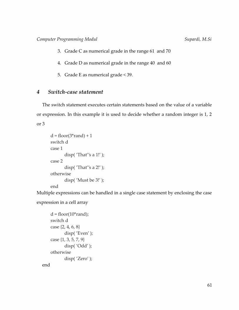
4 Switch-case statement
The switch statement executes certain statements based on the value of a variable
or expression. In this example it is used to decide whether a random integer is 1, 2
or 3
d = floor(3*rand) + 1switch dcase 1
disp( ’That’’s a 1!’ );case 2
disp( ’That’’s a 2!’ );otherwise
disp( ’Must be 3!’ );end
Multiple expressions can be handled in a single case statement by enclosing the case
expression in a cell array
d = floor(10*rand);switch dcase {2, 4, 6, 8}
disp( ’Even’ );case {1, 3, 5, 7, 9}
disp( ’Odd’ );otherwise
disp( ’Zero’ );end
61
Computer Programming Modul Supardi, M.Si
Exercise 4.
Write a computer program to compute (1) area of a circle, (2) area of square
(bujur sangkar) and (3) area of rectangle (persegi panjang). In this program, you must
set if your input is 1, it means that you must calculate the area of circle. Similarly, if
your input is 2, so you calculate the area of bujursangkar, and so on.
`
62

Computer Programming Modul Supardi, M.Si
CHAPTER 7
LOOPING
So far we have seen how to get data into a program, how to do arithmetic,
and how to get some answers out. In this section we look at a new feature:
repetition. This is implemented by the extremely powerful for construct. We will
first look at some examples of its use, followed by explanations. For starters, enter
the following group of statements on the command line. Enter the command format
compact first to make the output neater:
for i = 1:5, disp(i), end
Now change it slightly to
for i = 1:3, disp(i), end
And what about
for i = 1:0, disp(i), end
Can you see what’s happening? The disp statement is repeated five times, three
times, and not at all.
Square rooting with Newton
The square root x of any positive number a may be found using only the
arithmetic operations of addition, subtraction and division, with Newton’s method.
This is an iterative (repetitive) procedure that refines an initial guess. The structure
plan of the algorithm to find the square root, and the program with sample output
for a = 2 is as follows. Run it.
1. Initialize a
63
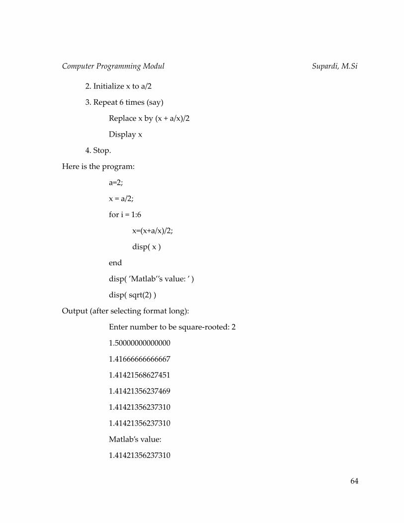
Computer Programming Modul Supardi, M.Si
2. Initialize x to a/2
3. Repeat 6 times (say)
Replace x by (x + a/x)/2
Display x
4. Stop.
Here is the program:
a=2;
x = a/2;
for i = 1:6
x=(x+a/x)/2;
disp( x )
end
disp( ’Matlab’’s value: ’ )
disp( sqrt(2) )
Output (after selecting format long):
Enter number to be square-rooted: 2
1.50000000000000
1.41666666666667
1.41421568627451
1.41421356237469
1.41421356237310
1.41421356237310
Matlab’s value:
1.41421356237310
64

Computer Programming Modul Supardi, M.Si
The value of x converges to a limit, which is √a. Note that it is identical to the value
returned by MATLAB’s sqrt function. Most computers and calculators use a similar
method internally to compute square roots and other standard mathematical
functions.
Factorials!
Run the following program to generate a list of n and n! (spoken as ‘n factorial’, or
‘n shriek’) where
n! = 1 × 2 × 3 × ... × (n − 1) × n.
n = 10;
fact = 1;
for k = 1:n
fact = k * fact;
disp( [k fact] )
end
Do an experiment to find largest value of n for which MATLAB can find n factorial
(you’d better leave out the disp statement!).
The basic for construct
In general the most common form of the for loop (for use in a program, not on the
command line) is
for index = j:k
statements
end
or
for index = j:m:k
65

Computer Programming Modul Supardi, M.Si
statements
end
Note the following points carefully:
1. j:k is a vector with elements j, j + 1,j + 2,...,k.
2. j:m:k is a vector with elements j, j + m, j + 2m,..., such that the last element
does not exceed k if m> 0, or is not less than k if m< 0.
3. index must be a variable. Each time through the loop it will contain the next
element of the vector j:k or j:m:k, and for each of these values statements
(which may be one or more statement) are carried out.
The for statement in a single line
If you insist on using for in a single line, here is the general form:
for index = j:k, statements, end
or
for index = j:m:k, statements, end
Note:
1. Don’t forget the commas (semi-colons will also do if appropriate). If you
leave them out you will get an error message.
2. Again, statements can be one or more statements, separated by commas or
semi-colons.
3. If you leave out end, MATLAB will wait for you to enter it. Nothing will
happen until you do so.
Exercise 1.
Create a computer program to calculate ∑n=1
1000
n with the for statement.
66

Computer Programming Modul Supardi, M.Si
Exercise 2.
Create a computer program to calculate the series with alternating sign
1−12+ 1
3−1
4+⋯+1
n where n=999 with the for statement.
The while Statement.
The while loop is used in cases where the looping process must terminate
when a specified condition is satisfied, and thus the number of passes is not known
in advance. A simple example of a while loop is
x = 5 ;
k = 0 ;
while x < 25
k = k + 1 ;
y(k ) = 3 *x;
x = 2 *x -l ;
end
The loop variable x is initially assigned the value 5, and it keeps this value
until the statement x = 2*x - 1 is encountered the first time. Its value then changes to
9. Before each pass through the loop, x is checked to see if its value is less than
25. If so, the pass is made. If not, the loop is skipped and the program
continues to execute any statements following the end statement. The variable x
takes on the values 9, 17, and 33 within the loop. The resulting array y contains
the values y (1) = 15, y ( 2) = 27, y ( 3) = 51.
Example
67

Computer Programming Modul Supardi, M.Si
Create a computer program, when algoritm of the program is given. Here is the
algoritm
1. Generate random integer
2. Ask user for guess
3. While guess is wrong:
If guess is too low
Tell her it is too low
Otherwise
Tell her it is too high
Ask user for new guess
4. Polite congratulations
5. Stop.
Example.
Create a computer program to make an arragement of number shown below
1
1 2
1 2 3
1 2 3 4
1 2 3 4 5
1 2 3 4 5 6
Exercise 3.
68
Computer Programming Modul Supardi, M.Si
Make a program to calculate the series of number shown below
−1+1/3−1/5+1 /7−1/9+⋯
until the final term less than 10−10 .
69

Computer Programming Modul Supardi, M.Si
MODUL 8
BREAK AND CONTINUE
break
The break statement will terminate execution of a for loop or while loop
Syntaxbreak
Description
The break statement will terminate the execution of a for or while loop.
Statements in the loop that appear after the break statement are not executed. In
nested loops, break exits only from the loop in which it occurs. Control passes to the
statement that follows the end of that loop.
Remarks
The break statement is not defined outside a for or while loop. Use return in this
context instead.
Examples
N=20;
for i=1:N
if (i>5)
break;
end
fprintf('%i. I am a student at UNY \n',i);
70

Computer Programming Modul Supardi, M.Si
end
The break statement at the above program will exit the for loop when i>5 is
encountered. In other word, the sentence “ I am a student at UNY” will not be
displayed when i=6.
Exercise 1.
Create a Matlab program to calculate the sumation as below
−1+1/3−1/5+1 /7−1/9+⋯
until the last term is less than 10−4 . Following is algoritm of the program
(1) initialize jum=0,
(2) determine the constant tol=10−4 , N=10000000
(3) initialize sign=1
(4) initialize term=1
(5) Repeat N times, starting from k=1
➔ sign=-sign
➔ term=1/(2*k-1)
➔ if term<tol
➔ stop
➔ jum=jum+sign*term
(6) display the result
(7) end
continue
The continue statement will pass control to the next iteration of FOR or
71

Computer Programming Modul Supardi, M.Si
WHILE loop in which it appears, skipping any remaining statements in the body
of the FOR or WHILE loop. In nested loops, CONTINUE passes control to the next
iteration of FOR or WHILE loop enclosing it.
Example.
N=20;
for i=1:N
if (i>5)
continue;
end
fprintf('%i. I am a student at UNY \n',i);
end
Exercise 2.
Calculate the series of number as shown below
1+1/ 2+1/ 4+1/6+1/8+⋯
and the program will be stoped after the final summation is greater than 6 and how
many terms of the series are?
Exercise 3.
Below is shown part of Matlab script
if a>b
if c>a
tmp=c;
else
tmp=a;
72

Computer Programming Modul Supardi, M.Si
end
else
if c>b
tmp=c;
else
tmp=b;
end
end
fprintf(tmp)
If a=2, b=4 and c=5, determine the final value of variable tmp.
Exercise 4.
Here is an algoritm which will display the variable N,P and E. Create a
program based on the algoritm
• initialize A=1 and N=6
• Repeat 10 times
• replace N with 2N
• suppose L=NA/2 and U=L1−A2/2
• suppose P=(U+L)/2
• suppose E=(U-L)/2
• displayN,P,E
• End
73
Computer Programming Modul Supardi, M.Si
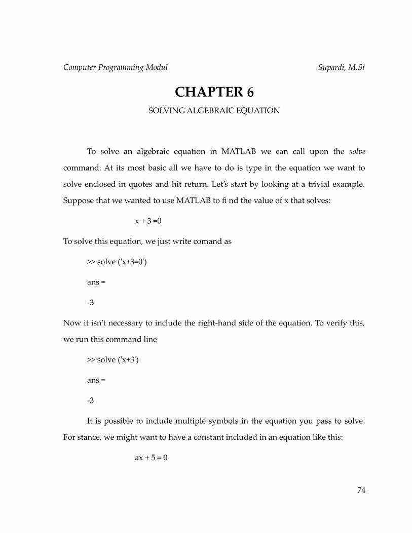
CHAPTER 6SOLVING ALGEBRAIC EQUATION
To solve an algebraic equation in MATLAB we can call upon the solve
command. At its most basic all we have to do is type in the equation we want to
solve enclosed in quotes and hit return. Let’s start by looking at a trivial example.
Suppose that we wanted to use MATLAB to fi nd the value of x that solves:
x + 3 =0
To solve this equation, we just write comand as
>> solve ('x+3=0')
ans =
-3
Now it isn’t necessary to include the right-hand side of the equation. To verify this,
we run this command line
>> solve ('x+3')
ans =
-3
It is possible to include multiple symbols in the equation you pass to solve.
For stance, we might want to have a constant included in an equation like this:
ax + 5 = 0
74
Computer Programming Modul Supardi, M.Si
>> solve ('a*x+3=0')
ans =
-3/a
But, if we want to determine a specific variable in the equation. For example, we can
determine the variale a from the above equation by writing
>> solve ('a*x+3=0','a')
ans =
-3/x
Solving Quadratic Equation
The solve command can be used to solve higher order equations as quadratic
equation.
>> s=solve ('x^2+3*x-2=0')
s =
-3/2+1/2*17^(1/2)
-3/2-1/2*17^(1/2)
The alternative way to write command line is
>> d='x^2+3*x-2=0';
>> s=solve (d)
s =
75
Computer Programming Modul Supardi, M.Si
-3/2+1/2*17^(1/2)
-3/2-1/2*17^(1/2)
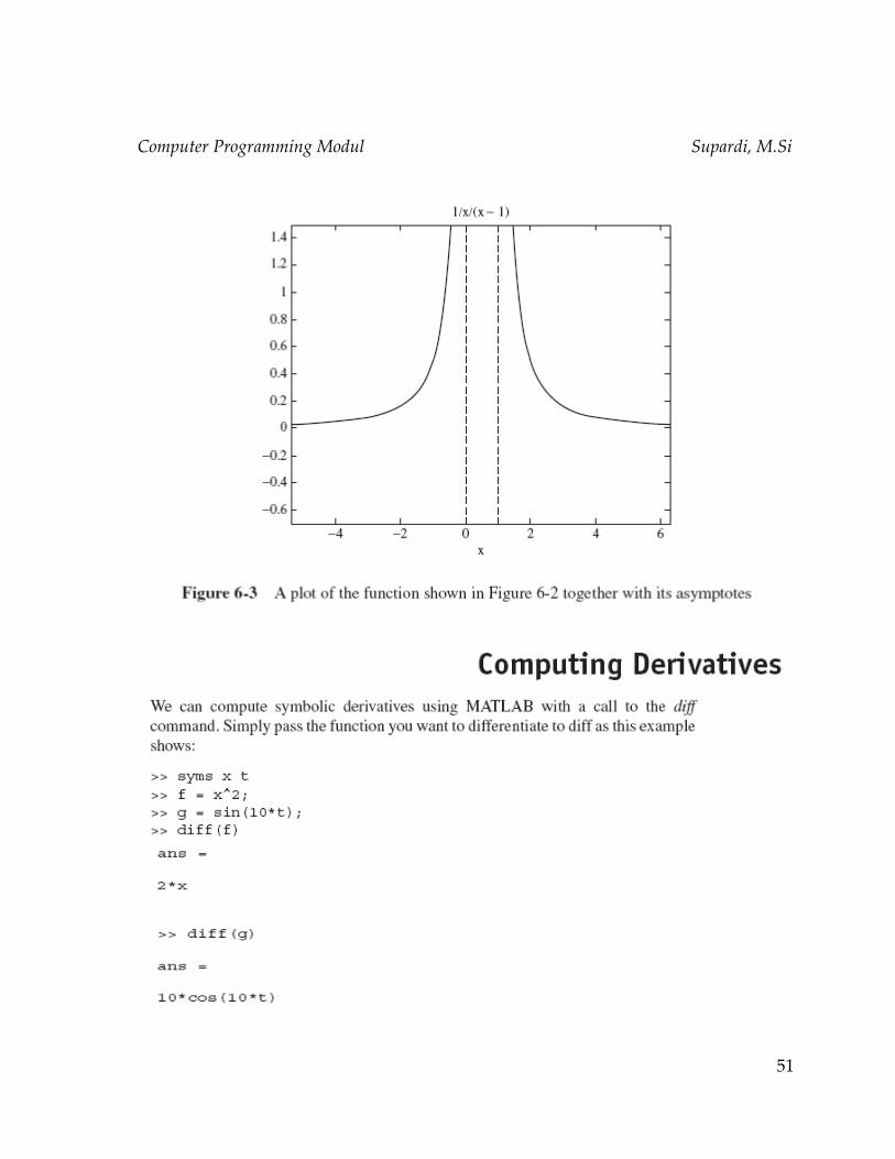
Plotting Symbolic Equation
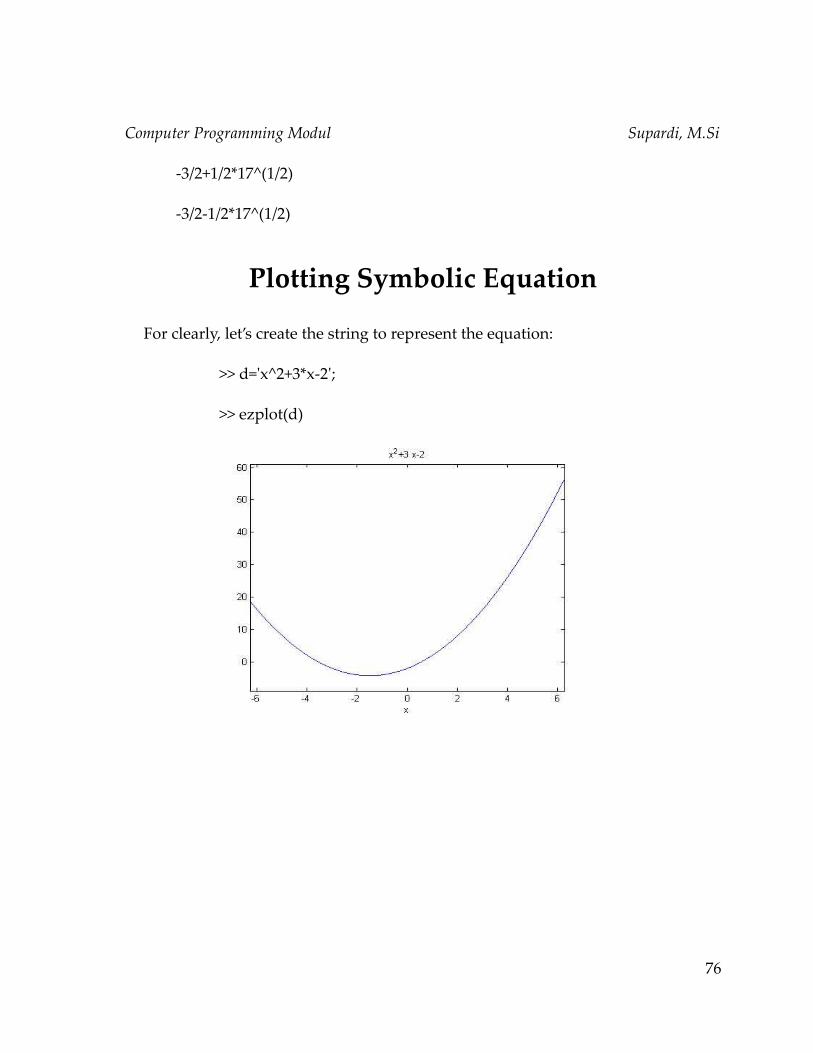
For clearly, let’s create the string to represent the equation:
>> d='x^2+3*x-2';
>> ezplot(d)
76
MODULE
COMPUTER PROGRAMMING
by:Supardi, M.Si
DEPARTMENT OF PHYSICS EDUCATIONFACULTY OF MATHEMATICS AND NATURAL SCIENCES
YOGYAKARTA STATE UNIVERSITY2011
Related Documents